Prediction of Airfoil Icing and Evaluation of Hot Air Anti-Icing System Effectiveness Using Computational Fluid Dynamics Simulations

Abstract

Icing poses a serious threat to flight safety, and ice accretion simulations are essential for addressing aircraft icing problems. In ice accretion prediction, systematic research covering all icing conditions based on actual flight phases is lacking, and the performance of anti-icing systems has not been investigated. In this study, maximum ice thickness prediction models for airfoils considering all flight phases were developed, and the performance of hot air anti-icing systems was analyzed. A hot air anti-icing system model was established, and the anti-icing effectiveness of the system under severe icing conditions was evaluated via conjugate heat transfer (CHT) calculations. The calculation results showed that during climbing above 10,000 ft under glaze ice conditions, the maximum ice thickness reached 13.47 mm at −6 °C, with a median volumetric diameter (MVD) of 20 μm. Under rime ice conditions, the maximum thickness exhibited linear relationships with the icing parameters, remaining below 5 mm. The calculation results revealed nonlinear relationships between maximum ice thickness on the airfoil leading edge and the icing conditions. Ice thickness models were established via polynomial regression. The maximum ice thickness data were classified, and 15 regression models were obtained. The relative errors between the predicted and calculated values remained below 3%, demonstrating high predictive accuracy. These models were employed to estimate the effectiveness of piccolo tube hot air anti-icing systems under the most severe icing conditions. The results indicated that 100% anti-icing efficiency was achieved at high ambient temperatures (above −10 °C). During takeoff, holding, and climbing phases with a high speed of 154.3 m/s, the system may face challenges in maintaining anti-icing protection, resulting in runback ice with a maximum thickness exceeding 5 mm.

1. Introduction

Aircraft icing occurs during flight in clouds at temperatures at or below freezing when supercooled water droplets impinge on and freeze on unprotected areas [1]. Ice accretion on critical components of aircraft, such as the airfoil leading edge and control surfaces, adversely affects the aerodynamic shape of aircraft. This deterioration in the aircraft’s aerodynamic profile leads to decreased lift, thus reducing flight stability and potentially resulting in accidents [2,3]. Research on ice accretion on aircraft surfaces is crucial for evaluating the performance of iced aircraft and developing effective de/anti-icing strategies [4]. Various anti-icing techniques have been established to mitigate the detrimental effects of possible ice accretion. One of the most widely employed thermal anti-icing techniques is hot air anti-icing [5], which involves the use of bleed air from the compressor stage of engines in modern airliners. Notably, bleed air, which exhibits medium-to-high temperatures and pressures, is exhausted through jet holes on the piccolo tube to heat lifting surfaces and prevent ice accretion [6].

Different icing conditions are associated with various types of ice accretion; depending on the icing mechanism, ice accretion can be classified as rime ice, glaze ice, or mixed ice [7]. Supercooled water droplets freeze instantaneously upon impact to form rime ice or flow as water back along the airfoil to form glaze ice [8]. Rime ice usually occurs at low temperatures and low liquid water contents, whereas glaze ice is formed at higher temperatures under freezing conditions and high liquid water contents. Mixed ice is defined as a mixture of rime and glaze ice types.

These forms of ice accretion can be investigated through various approaches, including flight tests, experimental simulations [9,10], engineering methods [11], and numerical simulations [12,13]. The exact ice shape can be determined through flight tests and experimental simulations. However, these approaches are usually too expensive to be widely adopted. In engineering methods, typical experimental data and empirical models are used. However, such approaches cannot be applied to analyze the ice accretion process accurately. Therefore, with the continuous advancement of computational fluid dynamics (CFD), numerical simulation has emerged as a popular technique in aircraft icing and de/anti-icing research because of the cost-effectiveness and efficiency of this approach [14,15,16]. Ice accretion simulations typically involve three steps: (1) flow determination, (2) droplet trajectory calculation, and (3) thermodynamic/freezing process analysis [17]. The air flow field can be obtained through the panel method or vortex lattice method [18]; alternatively, the potential flow equation [19], Euler equation or Navier–Stokes equations can be solved [20]. The droplet collection efficiency on the airfoil surface can be calculated via droplet trajectory simulations, which are important in numerically simulating ice accretion, and two computational methods are available: the Lagrangian method and the Eulerian two-phase flow method [21]. In the Lagrangian method, which is used in models such as LEWICE [22] and ONERA [23], a single droplet is adopted as the research object. In the Eulerian method, which has been applied in FENSAP-ICE [24], the continuous distribution of droplets in space is adopted as the research object. By solving the governing equation of the water phase, the distributions of the mass and airspeed of the droplets in the airflow field can be calculated, and the droplet collection coefficient of the icing surface can be obtained.

However, three-dimensional viscous turbulent aero-icing simulations are computationally expensive, especially for certification campaigns when broad parametric studies are needed [25]. To reduce the computational costs of complex icing simulation calculations, machine learning-based icing prediction methods [26] have gradually emerged as accurate alternatives. For example, Strijhak et al. [27] employed artificial neural networks to predict ice accretion for different airfoils. The input target data for neural networks include data on airfoil and ice geometries, which are transformed into a set of parameters, and the input features include physical flow parameters. However, the data used for prediction are limited and do not cover all the icing conditions included in FAR part 25 Appendix C for icing envelopes [28].

Fossati et al. [25] presented a reduced-order modeling methodology based on proper orthogonal decomposition and Bayesian kriging interpolation techniques to predict ice shapes. Messegur et al. [29] proposed a framework for the development of low-dimensional models for the prediction of ice profiles and associated aerodynamic performance degradation. Li et al. [30] introduced a purely data-driven approach to obtain complex patterns under different flight conditions for aircraft icing severity prediction and applied a learning-enabled extreme gradient boosting algorithm to establish a prediction framework based on an arbitrary set of observations. The results revealed that the proposed method could be used to evaluate aircraft icing severity. The authors selected numerous sample points to explore the icing meteorological conditions within the continuous maximum icing envelope, including the temperature, median volumetric diameter (MVD), and liquid water content (LWC). However, it remains challenging to consider all potential icing conditions across realistic phases when considering flight condition parameters such as airspeed and altitude. Therefore, further research is needed on prediction methods that comprehensively account for both meteorological and flight parameters across all practical flight phases.

In the analysis of heat transfer in thermal ice protection systems, the results obtained with an anti-icing simulation procedure based on the conjugate heat transfer (CHT) method, which involves the use of modules in the in-flight icing package FENSAP-ICE, have been validated against experimental results [31]. Silva et al. [32] employed electrothermal deicing modeling and simulations to predict the temperature and runback water flow’s streamwise distribution on an airfoil surface. Yang [33] developed an optimization method for aircraft hot gas anti-icing systems on the basis of a reduced-order method, and the established method was applied to obtain the distributions of the surface temperature and return water. Abdelghany et al. [34] proposed an approach based on machine learning and the Internet of Things (IoT) to predict the thermal performance characteristics of wing hot air anti-icing systems, and the artificial neural network (ANN) prediction results were compared with experimental data and CFD data. The multiple error results verified the efficiency of the approach.

In contrast to surface temperature and return water distribution, runback ice thickness is a more direct and tangible indicator of the effectiveness of anti-icing systems. For example, Lee et al. [35] verified the effectiveness of a new composite material-based electrothermal anti-icing system through experiments and compared the experimental results with runback ice accretion simulation results. Jung et al. [36] developed a meta model to evaluate the performance of electrothermal anti-icing systems for rotorcraft engine air intakes on the basis of surface ice thickness, temperature, and MVD distribution contours. The authors adopted a uniform sampling approach at four temperatures over the continuous maximum icing envelope to choose the icing samples. However, recent anti-icing studies typically use randomly selected icing conditions and lack systematic investigation under extreme icing conditions.

Therefore, this study presents a prediction approach to estimate the maximum ice thickness on aircraft wings under practical flight conditions. The selection of icing parameters accounts for all the flight phases and icing conditions covered by the continuous maximum icing envelope in FAR part 25 Appendix C. The data were fitted with a polynomial regression function to obtain mathematical models of the maximum icing thickness during each flight phase for different types of ice, and the models were then applied to calculate the most severe icing conditions. A hot air anti-icing system with a piccolo tube was subsequently established, and CHT calculations were performed with the most severe icing conditions set as the external flow conditions. Finally, the anti-icing effectiveness of the system was evaluated on the basis of the calculation results.

2. Calculation Methods and Validation Cases

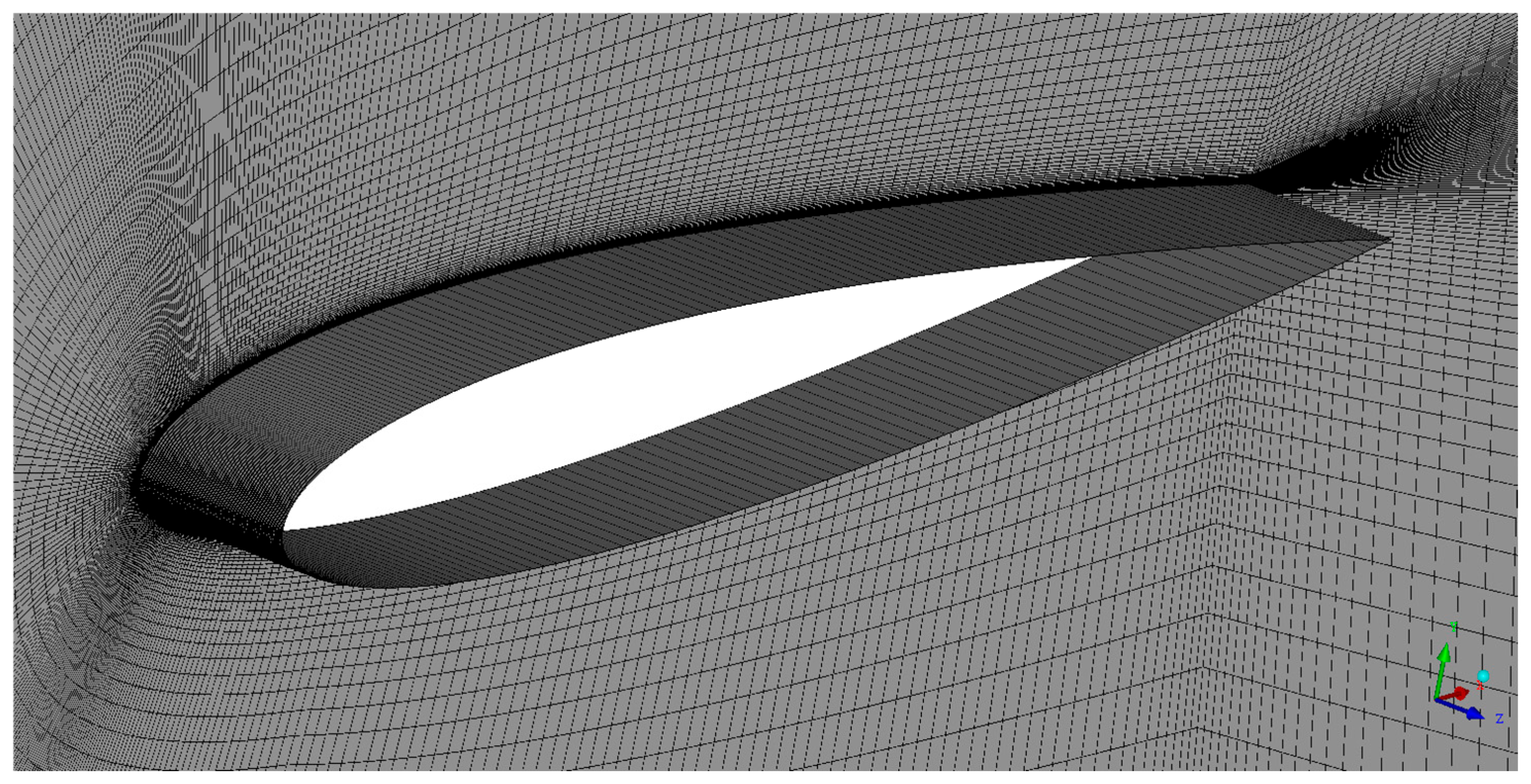
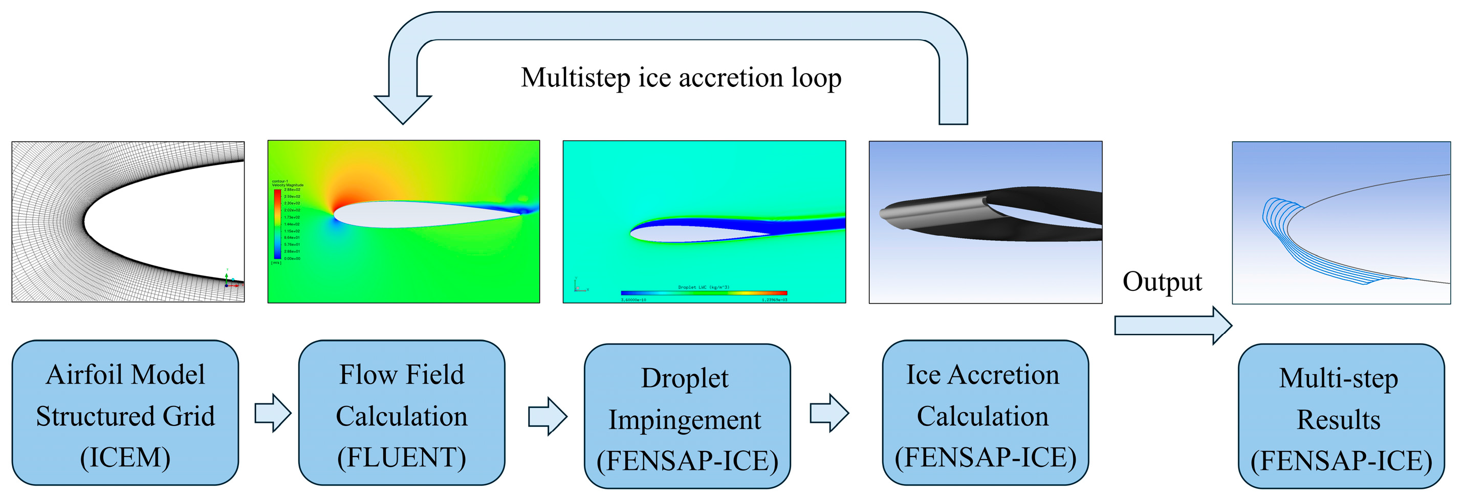
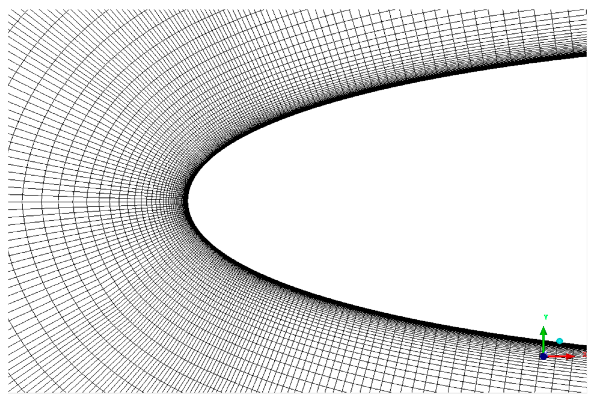
2.1. Computational Approaches

Three-dimensional icing simulations of the NACA 0012 airfoil were conducted using ANSYS 2022 R1 software, which included ICEM, FLUENT, and FENSAP-ICE. The simulation procedure was as follows: first, a computational grid was generated with ICEM software. Second, the flow field was computed. Third, droplet impingement and ice accretion calculations were performed. The airflow solution was obtained independently in FLUENT, while droplet impingement and ice accretion were calculated in FENSAP-ICE. The finite element Navier–Stokes code, coupled with a Eulerian-based algorithm in FLUENT and FENSAP-ICE, was used to compute the flow field and droplet impingement. The ice accretion algorithm was based on the heat transfer between the exposed surface and the thin water film formed by droplet impingement.

Multistep Computation

For a given mesh, flight conditions, and icing conditions, the solver was first utilized to perform flow analysis. Then, droplet impingement on the surface was calculated, and an ice profile was calculated without remeshing for a chosen partial exposure time. These steps were employed for single-step ice accretion calculations. To obtain more accurate ice shape characteristics, a multistep approach is necessary. In this method, the NACA 0012 grid was remeshed following each ice accretion calculation. This process was repeated iteratively to simulate ice accretion over time. Ice accretion was analyzed via a quasisteady iterative approach (Figure 1).

As shown in Figure 1, the simulations using the different icing software packages must be conducted in a strictly sequential manner. The flow field must first be computed through the use of an appropriately defined mesh. After completing the flow field calculation in FLUENT, the droplet properties are assigned in FENSAP-ICE to conduct droplet impingement analysis. Ice accretion can only be computed based on the droplet impingement results. The calculation results are transferred manually between the different software packages in a unidirectional manner. A simulation loop is completed after multistep ice accretion calculation, and in the next simulation step, the conditions for the flow field, droplet impingement, and ice accretion calculation must be reentered.

The Reynolds-averaged Navier–Stokes (RANS) equations were solved using the pressure-based solver in FLUENT with a coupled pressure–velocity algorithm. The spatial discretization process relies on the use of a least-squares cell-based method for gradients, a second-order scheme for pressure, and second-order upwind schemes for the other terms (density, momentum, turbulence, and energy). Boundary conditions included a constant-temperature wall, far-field pressure, and a symmetry plane. Droplet impingement and ice accretion were computed using FENSAP-ICE.

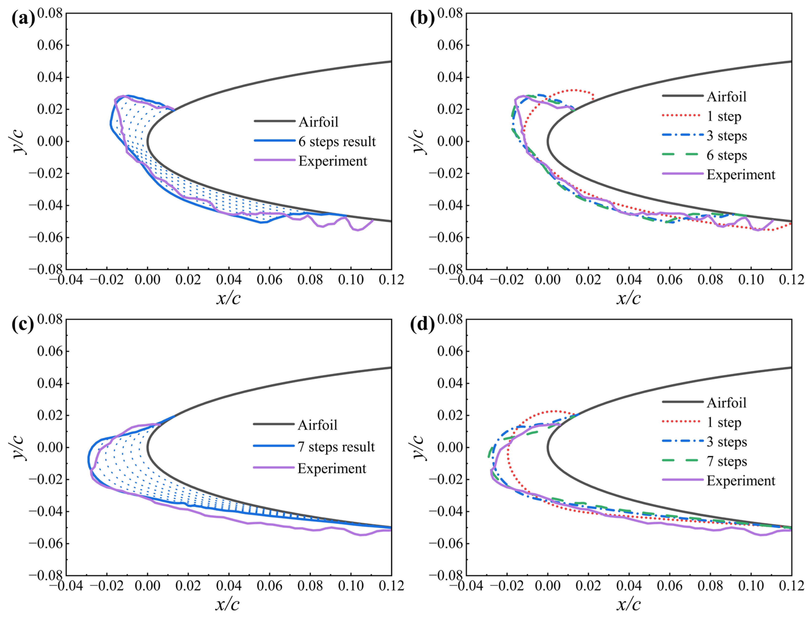
2.2. Example Analysis and Validation

To verify the effectiveness of the model, numerical simulations were conducted under the selected icing conditions. The simulation results were compared with the experimental data obtained by NASA [10,37,38], and the calculation conditions were consistent with the conditions in the experiment. The NACA 0012 airfoil was selected as the simulation model, with a chord length of 0.5334 m. The computational conditions are listed in

Table 1. Icing calculation conditions.

Case	AOA (°)	${\mathit{V}}_{\mathbf{\infty }}$ (m/s)	LWC (g/m3)	MVD (μm)	${\mathit{T}}_0$ (°C)
1	4.0	67.05	1.0	20	−2.22
2	4.0	102.82	0.55	20	−26.11

. The altitude in the calculation cases was set to 0 m, corresponding to an atmospheric pressure of 101,300 Pa. Additionally, the value of the ice accretion time parameter was set to 360 s in Case 1 and 420 s in Case 2. The calculation process included grid generation, flow field calculation, droplet trajectory calculation, and ice accretion calculation steps. A multistep method was used in the calculation process, and the ice accretion time interval was divided into equal intervals.

Figure 2 shows a C-type computational grid with approximately 114,700 grid nodes developed using ICEM software. A structured grid was employed, with the external domain extending 20 chord lengths from the airfoil. A grid refinement process was applied near the leading edge, where the minimum spacing between adjacent nodes was 0.3 mm. The height of the first boundary layer was set to 10⁻⁶ m, ensuring that the y+ values were less than 1. For the turbulence model, the k-ω shear stress transport (SST) model was adopted, with the far-field turbulence intensity set to 1% and the turbulence viscosity ratio μ_t/μ = 10⁻⁵. For a chord-based Reynolds number of 10⁶, the surface roughness was defined as 0.5 mm, and sand grain roughness distributions were dynamically obtained during icing.

The computational data were normalized to yield dimensionless icing morphology data for the wing. A comparison of the simulation and experimental results is shown in Figure 3. As shown in Figure 3a, typical glaze ice accretion is predicted due to the high environmental temperature (−2.22 °C). Moreover, for both the calculated and experimental ice shapes, a horn is observed on the upper surface. This occurs because the supercooled droplets do not freeze immediately upon impact. Instead, many of the supercooled droplets flow across the surface in the form of liquid water and freeze gradually. As shown in Figure 3c, at a lower environmental temperature (−26.11 °C), the droplets freeze instantaneously at their impingement locations, resulting in distinct characteristics of rime ice accretion. The multistep simulation results, as shown in Figure 3a,c, closely match the experimental results, demonstrating the high accuracy of the simulations.

In general, increasing the number of steps results in reduced mesh quality and an increased calculation time. To investigate the effect of step number on the simulated ice profile, icing calculations were performed with 1-, 3-, 6-, and 7-step approaches, and the results were compared with the experimental results. Figure 3b shows the predicted ice shapes for the 1-, 3-, and 6-step simulations under glaze ice conditions, while Figure 3d shows the corresponding results for the 1-, 3-, and 7-step simulations under rime ice conditions. The comparison reveals that further increasing the number of steps beyond three has only a marginal effect on the predicted ice location and shape. On this basis, the subsequent simulations were conducted using the 3-step approach to balance accuracy and computational efficiency. Furthermore, according to the A320 aircraft maintenance manual, the chord length of the wingtip is 1.5 m. Therefore, the original airfoil model was scaled to a chord length of 1.5 m. For this chord length, the Reynolds number reaches 10⁷. A 3D C-type computational grid with approximately 114,700 grid nodes was adopted, as this configuration yielded an ice shape error smaller than 10% between the numerical and experimental data.

3. Icing Conditions and Calculation Results

In this section, the airfoil icing conditions, including both flight conditions and meteorological icing conditions, used in the calculations are described. According to airworthiness regulations and related documents, six key parameters should be considered in aircraft icing studies. These include three meteorological icing parameters, namely, temperature, MVD, and LWC, and three flight icing parameters, namely, altitude, airspeed, and angle of attack (AOA). To investigate the realistic flight and meteorological conditions that occur when an aircraft encounters clouds with supercooled water droplets during flight, data from FAR part 25 Appendix C [28], the Airbus flight operation manual [39], and ICAO documents 8168-OPS/611 [40] were considered. To determine the flight speed and AOA conditions, the influences of the airspeed and AOA on the icing results were studied.

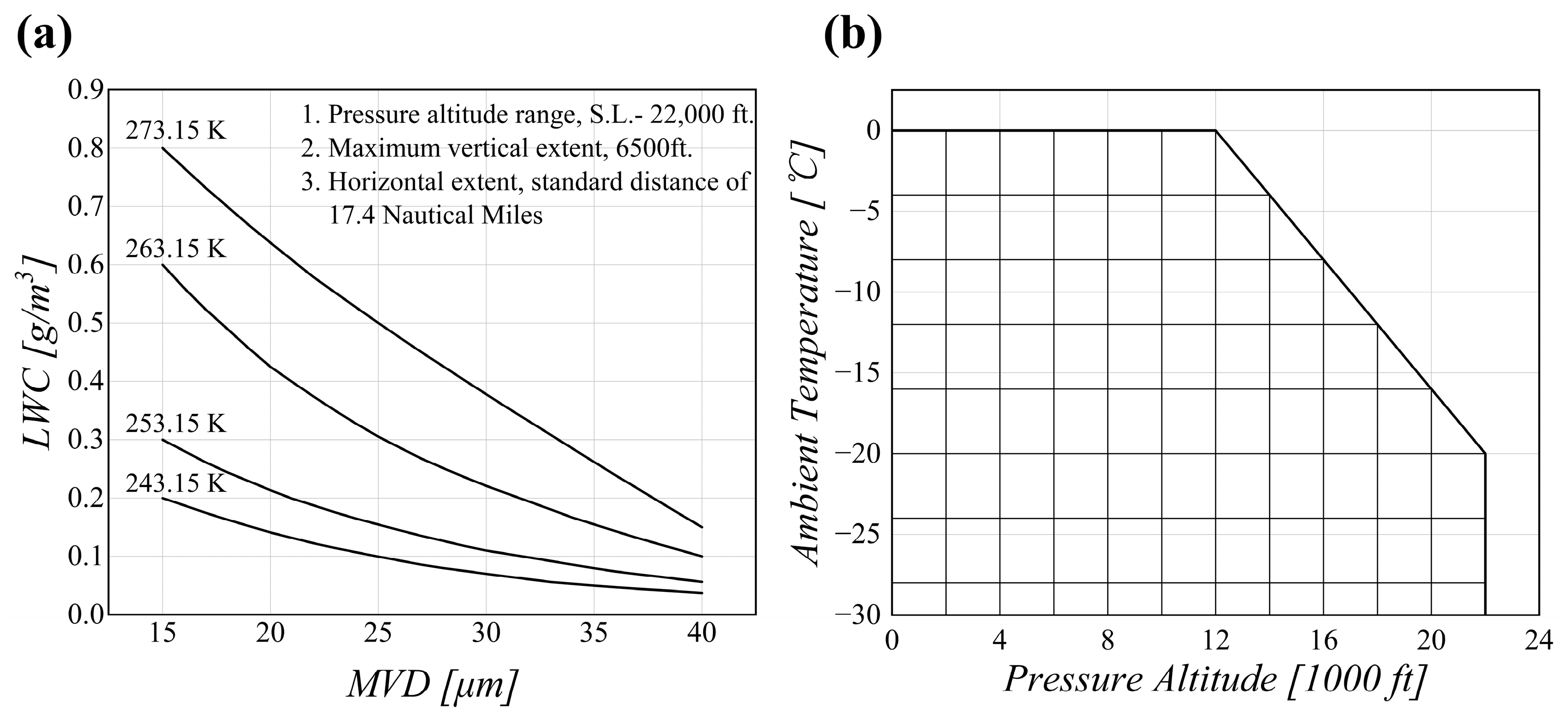
3.1. Icing Meteorological Conditions

Two types of envelopes are used to describe the icing conditions for aircraft certification in FAR part 25 Appendix C, namely, continuous maximum icing and intermittent maximum icing. Both envelopes are defined by the LWC, MVD, and ambient air temperature. In this study, the continuous maximum icing envelope was adopted. As shown in Figure 4a, this envelope defines an ambient temperature range from 273.15 to 243.15 K, represented by four isothermal curves. The horizontal axis indicates the MVD, which ranges from 15 to 40 μm, and the LWC typically decreases with increasing MVD. Therefore, the maximum value of the LWC is 0.8 g/m³, occurring at an MVD of 15 μm and a temperature of 273.15 K. Similarly, the minimum LWC value occurs at an MVD of 40 μm and a temperature of 243.15 K. Figure 4b shows the range of temperatures at different pressure altitudes under continuous maximum icing conditions. At altitudes above 12,000 ft, the maximum freezing temperature decreases with increasing altitude. Specifically, for every 1000 ft increase in altitude, the maximum freezing temperature decreases by 2 °C. This gradient was employed to determine the altitude and temperature parameters.

3.2. Flight Phases and Flight Conditions

The second part of FAR part 25 Appendix C indicates that ice accretion associated with aircraft performance and handling characteristics during each flight phase must be used to show compliance with the applicable airplane performance and handling requirements under icing conditions. The types of ice for the specified flight phases include takeoff ice (covering takeoff and final takeoff), en route ice (covering climbing and cruising), holding ice, approach ice, and landing ice. For takeoff ice, icing conditions between liftoff and 1500 ft above the takeoff surface must be considered. Since the continuous maximum icing envelope specifies a pressure altitude range from sea level to 22,000 ft, en route ice conditions at heights between 1500 and 22,000 ft were considered in this study, which corresponds to the climbing phase.

For the takeoff phase, the maximum limiting speed for the process from takeoff (from the ground) to accelerated climbing is considered, and the flight manuals for the A320 series indicate a maximum speed of up to 243 kt, with the flaps retracted at higher takeoff weights.

For the climbing phase, the Airbus operation manual indicates climbing at a given airspeed (IAS)/MACH trend [39], which was adopted to define the airspeed and altitude range. Taking A320 as an example, the climbing phase can be divided into two segments, namely, from 1500 ft to 10,000 ft, with a limited airspeed of 463 km/h (250 kt), and from 10,000 ft to 22,000 ft, with a maximum airspeed of 556 km/h (300 kt).

For the holding phase, standardized aircraft maneuvering criteria for instrument approach procedures are defined in ICAO Doc. 8168 OPS/611 Vol II [40]. The airspeeds for holding area construction are categorized on the basis of the altitudes of the holding areas: below 14,000 ft, an airspeed of 425 km/h (230 kt); from 14,000 to 20,000 ft, an airspeed of 445 km/h (240 kt); and from 20,000 ft to 34,000 ft, an airspeed of 490 km/h (265 kt).

For the approach and landing phases, five typical aircraft approach categories are established in Doc. 8168. Category C mainly refers to airliners such as the Boeing 737 series and the Airbus 319, 320, and 321 series. The airspeeds of Category C aircraft for the initial approach during the approach and landing phases vary between 295 and 445 km/h, the airspeeds for the final approach vary between 215 and 295 km/h, and the airspeeds for landing vary between 224 and 260 km/h.

Table 2. Altitude and airspeed ranges.

Flight Phase	Altitude (ft)	Airspeed (m/s)
Takeoff	$0\le H\le 1500$	$V_{\infty }\le 125$
Climbing below 10,000 ft	$1500<\mathrm{H}\le \mathrm{10,000}$	$V_{\infty }\le 128.6$
Climbing above 10,000 ft	$\mathrm{10,000}<\mathrm{H}\le \mathrm{22,000}$	$V_{\infty }\le 154.3$
Holding	$\mathrm{10,000}<\mathrm{H}\le \mathrm{22,000}$	$118\le V_{\infty }\le 136.3$
Approach and landing	$0\le \mathrm{H}\le \mathrm{10,000}$	$81.9\le V_{\infty }\le 123.5$ (initial approach) $59.7\le V_{\infty }\le 81.9$ (final approach) $62.2\le V_{\infty }\le 72.2$ (landing)

presents the altitude and airspeed ranges for the different flight phases for the A320 aircraft.

The above standards provide the maximum allowable speeds or speed ranges for aircraft during different flight phases. In contrast, there are no explicit regulations regarding the AOA. To determine the specific airspeed and AOA parameters, the impacts of these variables on ice accretion must be investigated.

3.3. Icing Conditions for Each Flight Phase

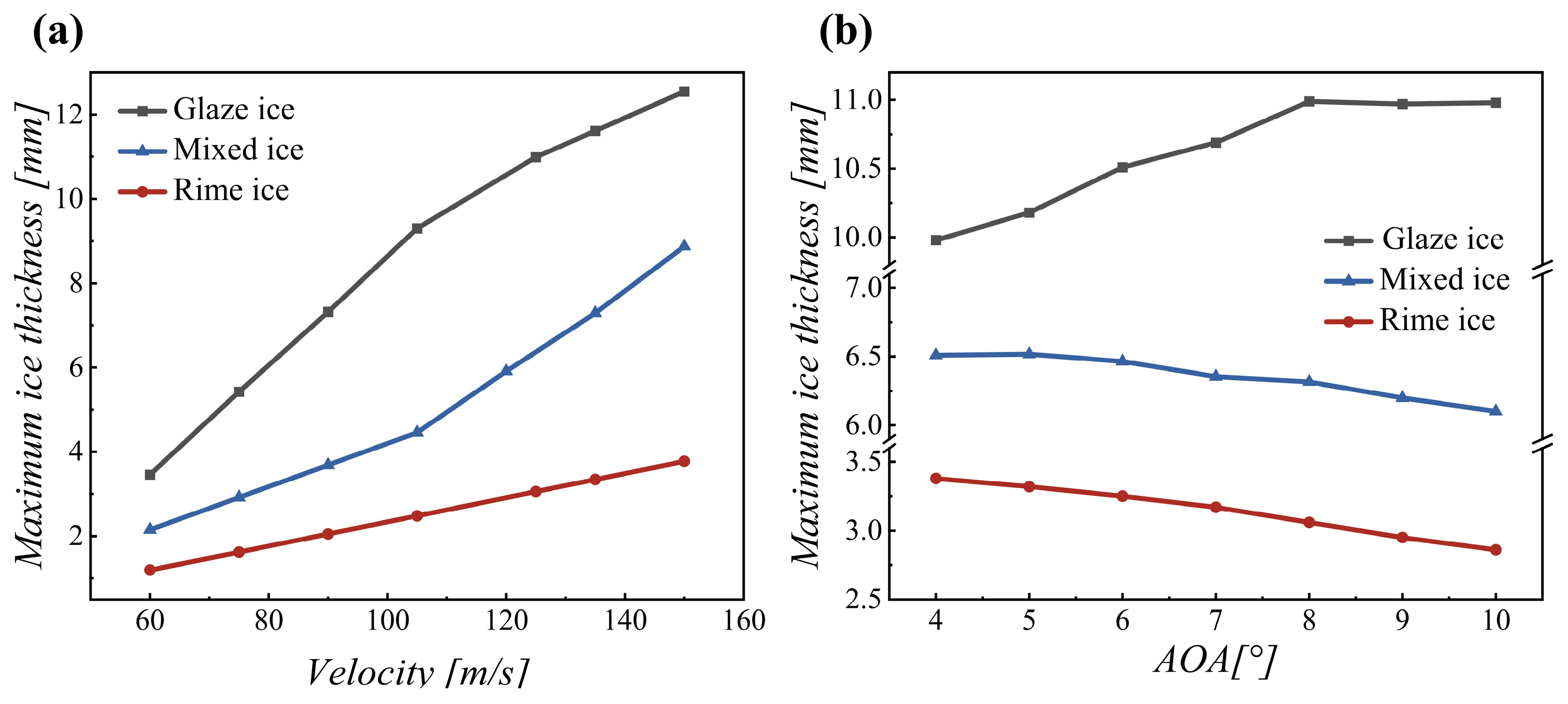
3.3.1. Influences of the Airspeed and Angle of Attack

Figure 5 shows the influences of the airspeed and AOA on the maximum ice thickness under glaze, mixed, and rime icing conditions. As shown in Figure 5a, the maximum ice thickness exhibits a velocity-dependent increasing trend across all three icing types. As the airspeed increases, the inertial of droplets increases, thereby enhancing impingement efficiency and ice accretion. This correlation is particularly linear in the case of rime ice, where rapid freezing confines ice accretion to the stagnation zone, thus minimizing nonlinearities caused by water runback. Figure 5b shows the influence of the AOA on the maximum ice thickness. Under glaze ice conditions, the maximum ice thickness initially increases with AOA, reaching a peak at 8°, beyond which it remains nearly constant. In contrast, under mixed and rime ice conditions, the maximum ice thickness consistently decreases with increasing AOA. However, the numerical results suggest that AOA exerts a relatively minor influence on the maximum ice thickness. Specifically, under glaze ice conditions, the maximum thickness increases gradually from 9.98 to 10.98 mm, corresponding to a 9.1% increase. Under mixed and rime ice conditions, the maximum thickness decreases by 6.3% and 15.04%, respectively.

3.3.2. Airfoil Icing Conditions

To develop mathematical models for predicting the maximum ice thickness on airfoils, appropriate airfoil icing conditions for all flight phases must be determined. The datasets used for model training and testing were generated through simulations. Owing to the high computational cost associated with full-stage airfoil icing simulations involving six variables, the number of icing parameters should be reduced without reducing the accuracy of the prediction model. In continuous maximum icing envelopes, each temperature and MVD combination yields a unique LWC value. This indicates that in stratiform clouds, the LWC and MVD values at a given temperature are correlated. In FENSAP-ICE software, the LWC value can be directly obtained from the FAR part 25 Appendix C icing envelope.

According to the previous analysis of the influences of airspeed and AOA on the maximum ice thickness on the airfoil, the ice thickness is greatest at the maximum airspeed. The most critical ice accretion for each flight phase must be considered according to FAR part 25 Appendix C, and the velocity was set as the maximum value for each flight phase. Notably, the approach and landing phases were grouped into a single operational interval. For the entirety of the approach and landing phases, the maximum airspeed was defined as the initial approach velocity of 123.5 m/s. Although the influence of the AOA on the maximum ice thickness varies across the different ice types, numerically, its overall effect is relatively minor. Considering that glaze conditions typically result in greater ice thickness, the AOA was set to 8°, corresponding to the maximum ice thickness under glaze ice conditions. The airfoil icing conditions for all the flight phases are listed in

Table 3. Airfoil icing condition parameters for all flight phases.

Flight Phase	$\mathbf{H}$ (1000 ft)	${\mathbf{V}}_{\mathbf{\infty }}$ (m/s)	${\mathbf{T}}_0$ (°C)	$\mathbf{M}\mathbf{V}\mathbf{D}$ (μm)	$\mathbf{L}\mathbf{W}\mathbf{C}$ (g/m3)	$\mathbf{T}\mathbf{i}\mathbf{m}\mathbf{e}$ (s)
Takeoff	0, 0.75, 1.5	125	−2, −6, −10	15 20 25 30 35 40	Determined on the basis of temperature and MVD in the continuous maximum icing envelope	258
	0, 0.75, 1.5		−10, −14, −18
	0, 0.75, 1.5		−20, −25, −30
Climbing below 10,000 ft	1.5, 5.5, 9.5 1.5, 5.5, 9.5 1.5, 5.5, 9.5	128.6	−2, −6, −10 −10, −14, −18 −20, −25, −30			250
Climbing above 10,000 ft	11, 12, 13 11, 14, 17 12, 16, 20	154.3	−2, −6, −10 −10, −14, −18 −20, −25, −30			210
Holding	11, 12, 13	136.3	−2, −6, −10			2700
	11, 14, 17		−10, −14, −18
	12, 17, 22		−20, −25, −30
Approach and landing	2, 6, 10	123.5	−2, −6, −10			260
	2, 6, 10		−10, −14, −18
	2, 6, 10		−20, −25, −30

. For the continuous maximum icing envelope, the standard horizontal distance was 17.4 nautical miles, and the icing accretion time was determined by dividing this distance by the airspeed. During the holding phase, the aircraft maintains a high altitude and stable speed, with prolonged exposure to low temperatures and potential icing, and the corresponding ice accretion time is 45 min (2700 s) [28].

3.4. Icing Simulation Results

In this section, trends in ice shapes are examined under different temperatures and MVD values, with particular focus on variations in the maximum ice thickness, which is an important indicator of the severity of airfoil icing. The icing severity based on the icing thickness was categorized into four levels [41]: light (0.1 to 5.0 mm), moderate (5.1 to 15 mm), heavy (15.1 to 30 mm), and severe (>30 mm). In moderate cases, even a very short period of icing may pose a threat to flight safety. In the A320 aircraft maintenance manual, an ice thickness of 5 mm is used as the criterion for classifying severe icing behavior. In addition, the temperature ranges for the different aircraft icing types are as follows: glaze ice (0 to −10 °C), mixed ice (−10 to −20 °C), and rime (−20 to −30 °C) [41].

Figure 6 shows the ice shapes under different icing conditions during the climbing phase at an altitude of 12,000 ft, with an airspeed of 154.3 m/s and an ice accretion time of 210 s. As shown in Figure 6, the ice shapes were influenced mainly by the environmental temperature, transitioning from horn-shaped glaze ice to smooth rime ice as the temperature decreased. The transition from horn-shaped ice to smooth ice profiles (Figure 6a–f) is intrinsically linked to the temperature distribution and freezing kinetics. At higher ambient temperatures (e.g., −2 to −10 °C), supercooled droplets partially retain their liquid state upon impact, forming glaze ice horns as unfrozen water flows upstream and gradually solidifies (Figure 6a–c). As the temperature decreases below −20 °C, rapid droplet freezing dominates due to enhanced heat transfer to the environment. The reduced liquid water runback distance confines ice accretion primarily to the impingement zone, resulting in homogeneous deposition and smooth rime ice formation (Figure 6e,f). Mixed ice is a mixture of rime and glaze ice types.

At glaze ice temperatures, as shown in Figure 6a–c, the runback phenomenon is notable, leading to distinct ice horn shapes. At −2 °C, as shown in Figure 6a, a higher LWC leads to more droplets flowing along the surface of the airfoil, resulting in an increased icing area and higher ice angle. At this temperature, the LWC decreases dramatically with increasing MVD. Furthermore, the kinetic energy of the droplets increases with increasing MVD, and the droplets flow farther along the surface of the airfoil. Therefore, under the combined influence of the LWC and MVD, the largest icing area occurs at an MVD value of 20 μm. At the other temperatures, the icing area gradually increases with increasing MVD. At temperatures of −6 and −10 °C, as shown in Figure 6b,c, respectively, the ice horn width gradually decreases, and the height increases, resulting in the formation of more prominent ice horn shapes. At the mixed ice temperature, as shown in Figure 6d, the runback phenomenon gradually disappears, causing both the width and height of the ice horns to decrease until they disappear, reflecting the transition from glaze ice to rime ice. At rime ice temperatures, as shown in Figure 6e,f, the droplets freeze rapidly upon impact with the airfoil surface, and the ice shapes become smooth and hornless.

Figure 7 shows the variation in the maximum ice thickness with the MVD at different ambient temperatures. Overall, with decreasing temperature, the LWC in clouds gradually decreases, which is accompanied by a reduction in the maximum ice thickness. Moreover, the maximum ice thickness decreases with increasing MVD since the LWC decreases with increasing MVD at the same temperature. However, at −2 °C, despite the higher LWC, the higher temperature results in more pronounced runback phenomena, resulting in an increased icing area and reduced ice thickness. As a result, relatively consistent maximum ice thicknesses between 6 and 7 mm were observed.

At −6 and −10 °C, under the combined influence of the LWC and MVD, the maximum ice thickness occurs at an MVD of 20 μm, with peak values of 13.47 and 13.07 mm, respectively. Under mixed and rime ice conditions, the ice thickness is influenced primarily by the LWC. With increasing MVD, the LWC decreases, leading to a corresponding reduction in the maximum ice thickness. When temperatures decrease below −20 °C, which is associated with rime ice conditions, droplets freeze almost instantaneously upon impact, resulting in uniformly thin ice layers. Under these conditions, the maximum ice thickness remains less than 5 mm for all MVD values, and a clear linear relationship between the maximum ice thickness and MVD is observed.

4. Ice Thickness Prediction Model Development and Verification

Since ice thickness is a crucial indicator for assessing the severity of airfoil icing and exhibits nonlinear relationships with various icing parameters, as described in the previous section, we employed polynomial regression to fit a mathematical model for ice thickness on the basis of the altitude, temperature, MVD, and LWC. These four variables serve as input features for the polynomial regression model, with the corresponding maximum ice thickness as the target. In this section, we describe the process of establishing airfoil maximum ice thickness models, followed by an analysis of the prediction results and errors to demonstrate the effectiveness of the proposed approach.

4.1. Ice Thickness Prediction Models Based on CFD Data

Models for predicting the maximum ice thickness on airfoils were derived using polynomial regression applied to CFD icing simulation data. The data were categorized into 15 datasets on the basis of five flight phases and three icing types. Polynomial regression was conducted separately for each dataset, and the inputs were the altitude, temperature, MVD, LWC, and calculated maximum ice thickness. The outputs were the coefficients of each independent variable in the polynomial models. To reduce complexity and avoid redundant models, polynomial regression was limited to a maximum degree of 2. The theoretical model of polynomial regression is provided in Appendix A.

The dataset was randomly split into training (80%) and testing (20%) subsets to evaluate the model’s performance effectively. A global model deployed for the whole icing envelope is the best approach to reduce the complexity of the model generation process [42]. All the flight phases were considered in the maximum ice thickness models generated on the basis of the CFD calculation and data fitting approaches. These models incorporate a comprehensive range of icing conditions, covering the continuous maximum icing envelopes. For example, the model for the climbing phase above 10,000 ft for glaze ice (−2 °C to −10 °C) conditions is given as:

$$\begin{array}{c}\begin{array}{c}\begin{array}{c}f\left(x_1,x_2,x_3,x_4\right)=193.5477-2.5864x_1+3.3641x_2-5.5387x_3\\ -294.6683x_4+0.1095x_1^2-0.0941x_2^2+0.0395x_3^2\\ +131.4334x_4^2+0.0495x_1{x}_2-0.0010x_1{x}_3-0.1862x_1{x}_4\\ -0.0961x_2{x}_3-5.7943x_2{x}_4+4.2874x_3{x}_4\end{array}\end{array}\end{array}$$

(1)

where $x_1, x_2, x_3, x_4$ and $f (x_1, x_2, x_3, x_4)$ are the input variables, corresponding to the altitude, temperature, MVD, LWC, and maximum ice thickness, respectively. Moreover, $c_{k_1{k}_2{k}_3{k}_4}$ is the coefficient, which is assigned distinct dimensional units for each term, ensuring that the product of each coefficient with its corresponding variables yields results expressed in millimeters, thus aligning the units across both sides of the equation. The coefficients of the models for the three ice types (glaze, mixed, and rime ice) across the five flight phases are given in

Table A1. Coefficients calculated for the linear term in the maximum ice thickness models.

Flight Phase	Ice Type	1	x1	x2	x3	x4
Takeoff	Glaze	384.4159	0.7945	12.1233	−14.007	−707.3222
	Mixed	14.0647	0.2289	2.0822	0.4305	121.8727
	Rime	1.5975	−0.032	−0.1422	−0.1609	19.1868
Climbing below 10,000 ft	Glaze	303.3042	0.228	8.2574	−11.0277	−549.6192
	Mixed	15.4574	−0.095	2.7835	0.8029	152.1168
	Rime	1.0561	0.0054	−0.1391	−0.1352	20.9728
Climbing above 10,000 ft	Glaze	193.5477	−2.5864	3.3641	−5.5387	−294.6683
	Mixed	125.972	−0.0726	7.358	−2.2136	−66.1643
	Rime	4.1092	0.0122	−0.0593	−0.1958	18.2349
Holding	Glaze	211.381	0.1236	5.2253	−6.788	−362.0233
	Mixed	114.4934	−0.0839	1.5344	−3.0998	−140.5761
	Rime	45.6082	0.0763	−0.4387	−2.1194	3.2703
Approach and landing	Glaze	359.8611	0.3235	11.4168	−13.0325	−666.1164
	Mixed	55.5489	−0.1298	3.7192	−0.7565	52.2447
	Rime	1.0434	0.005	−0.1415	−0.1377	20.8362

,

Table A2. Coefficients calculated for the quadratic term in the maximum ice thickness models.

Flight Phase	Ice Type	${\mathit{x}}_1^2$	${\mathbf{x}}_2^2$	${\mathit{x}}_3^2$	${\mathit{x}}_4^2$
Takeoff	Glaze	−0.0018	0.0288	0.1264	328.8846
	Mixed	0.0081	0.0285	−0.0131	−90.5186
	Rime	0.0012	−0.0022	0.0019	−20.8271
Climbing below 10,000 ft	Glaze	−0.0003	−0.005	0.0999	252.4877
	Mixed	0.0042	0.0336	−0.0209	−117.2068
	Rime	0	−0.0021	0.0016	−20.1184
Climbing above 10,000 ft	Glaze	0.1095	−0.0941	0.0395	131.4334
	Mixed	−0.0003	0.0688	−0.001	−8.8369
	Rime	−0.0001	−0.0018	0.0018	−18.3447
Holding	Glaze	0.0001	0.0125	0.0541	158.1472
	Mixed	−0.0018	−0.0386	0.017	41.3202
	Rime	−0.0005	−0.015	0.0208	−54.4345
Approach and landing	Glaze	−0.0037	0.028	0.1168	310.9552
	Mixed	0.0022	0.038	−0.0058	−58.2327
	Rime	0	−0.0022	0.0017	−20.2136

, and

Table A3. Coefficients calculated for the interaction term in the maximum ice thickness models.

Flight Phase	Ice Type	${\mathit{x}}_1{\mathit{x}}_2$	${\mathit{x}}_1{\mathit{x}}_3$	${\mathit{x}}_1{\mathit{x}}_4$	${\mathit{x}}_2{\mathit{x}}_3$	${\mathit{x}}_2{\mathit{x}}_4$	${\mathit{x}}_3{\mathit{x}}_4$
Takeoff	Glaze	0.0005	−0.017	−0.7545	−0.2403	−12.9427	13.1868
	Mixed	0.0024	−0.0051	−0.1582	−0.0292	1.4258	−2.7716
	Rime	−0.0005	0.0004	0.1994	0.0002	0.5854	0.4797
Climbing below 10,000 ft	Glaze	−0.0041	−0.0047	−0.1257	−0.1631	−9.3107	10.2246
	Mixed	0.0023	0.0014	0.4366	−0.0407	1.12	−4.0122
	Rime	0.0001	−0.0001	0.1126	0.0003	0.5264	0.4123
Climbing above 10,000 ft	Glaze	0.0495	−0.0010	−0.1862	−0.0961	−5.7943	4.2874
	Mixed	−0.0074	−0.0014	0.0649	−0.1096	−4.3194	−1.4623
	Rime	0.0001	−0.0002	0.101	−0.0009	0.4602	0.2757
Holding	Glaze	0.0155	−0.0001	0.3749	−0.1004	−6.1764	8.4468
	Mixed	−0.0072	0.0008	0.3468	−0.046	−2.6114	3.6869
	Rime	−0.0004	−0.0018	0.6548	−0.0081	2.3469	5.5221
Approach and landing	Glaze	0.001	−0.0056	−0.2068	−0.2245	−12.3401	12.4056
	Mixed	−0.0004	0.0023	0.3918	−0.0591	−0.1521	−2.1118
	Rime	0.0001	−0.0001	0.1135	0.0003	0.5312	0.4285

, respectively, in Appendix A.

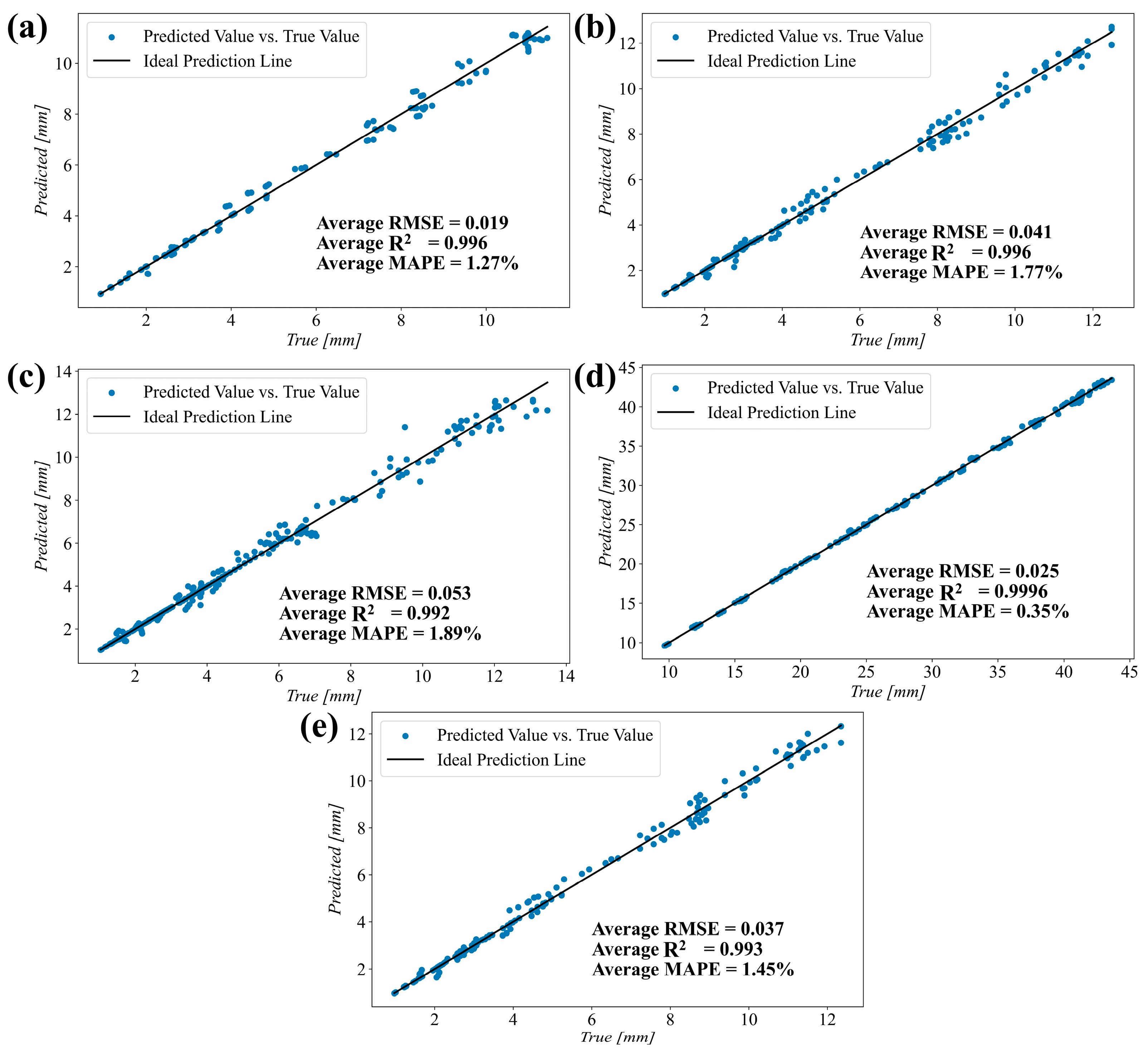
4.2. Performance Evaluation and Error Analysis

To evaluate the prediction results obtained with the proposed maximum ice thickness prediction models, the model performance was examined on the basis of several regression metrics. The mean square error ($MSE$), coefficient of determination ($R^2$), and mean absolute percentage error ($MAPE$) were used to evaluate the regression model results. The calculation formulas for the three error metrics are provided in Appendix B.

The test error results for the prediction models are listed in

Table 4. Errors of the test datasets.

Flight Phase	Ice Type	$\mathit{M}\mathit{S}\mathit{E}$	${\mathit{R}}^2$	$\mathit{M}\mathit{A}\mathit{P}\mathit{E}$
Takeoff	Glaze	0.0404	0.9900	1.63%
	Mixed	0.0163	0.9975	1.87%
	Rime	0.000113	0.999835	0.31%
Climbing below 10,000 ft	Glaze	0.1026	0.9893	2.93%
	Mixed	0.0211	0.9985	2.13%
	Rime	0.000098	0.999896	0.24%
Climbing above 10,000 ft	Glaze	0.1074	0.9806	2.71%
	Mixed	0.0513	0.9952	2.78%
	Rime	0.000049	0.999961	0.18%
Holding	Glaze	0.0527	0.9993	0.50%
	Mixed	0.0199	0.9996	0.33%
	Rime	0.0034	0.999946	0.21%
Approach and landing	Glaze	0.0976	0.9792	2.46%
	Mixed	0.0140	0.9989	1.63%
	Rime	0.000107	0.999887	0.25%

. According to the $MSE$ results, the maximum ice thickness prediction models for each ice type during all flight phases yield $MSE$ values lower than 0.1 except for the model for glaze ice conditions during the climbing phase. The $R^2$ metric indicates the variation between the input and output parameters, and all the prediction models provide successful results, with $R^2$ values very close to 1. The $MAPE$ criterion was used to assess the deviation between the true and predicted values. All the $MAPE$ values were lower than 3%. The error results revealed that the prediction accuracies of all the models were relatively high, with the highest accuracy for rime ice conditions.

To demonstrate the effectiveness of the models, a comparison of the predicted and true results for both the test and training datasets across all five flight phases is shown in Figure 8. A scatter plot was used to compare the true and predicted maximum ice thickness values, with a unit-slope line denoting ideal agreement. The x- and y-axis represent the true and predicted values, respectively. Close alignment of the data points with the line ($MAPE<3\mathrm{\%}$) confirms the model’s prediction accuracy across diverse icing conditions. As shown in Figure 8, the average $MSE$ values for all five flight phases are less than 0.1, the average $R^2$ values are greater than 0.99, and the average $MAPE$ values are less than 2%, indicating the high prediction accuracy of the polynomial regression model. As shown in Figure 8c, for the climbing phase above 10,000 ft, the highest average $MSE$ and $MAPE$ values and lowest $R^2$ values are 0.053, 1.89%, and 0.992, respectively. All the data points in the lower-left corner of the scatter plot represent relatively small true and predicted values, which vary between 0.9 and 4 mm, with correspondingly low prediction errors. These points correspond to rime ice conditions, where the ambient temperature is below −20 °C. Under such conditions, the ice thickness is directly proportional to the collected liquid water, which can be explained by the linear relationships between the maximum ice thickness and the associated icing parameters shown in Figure 7. In this case, the polynomial regression model provides a satisfactory fit because of the strong linear correlations between the maximum ice thickness and the icing parameters. The data points in the middle and upper-right portions of the scatter plot typically correspond to mixed and glaze ice conditions, respectively. Under these conditions, phenomena such as ice horns and runback water lead to more complex ice accretion patterns, resulting in irregular relationships between ice thickness and various icing parameters. These irregularities reduce the accuracy of the polynomial regression model. As shown in Figure 8d, during the holding phase, all the data points are close to the ideal prediction line. This can be attributed to the relatively large true and predicted maximum ice thickness values in this region, varying between 9.6 and 44 mm, resulting in a larger denominator in the relative error calculation, thereby reducing the relative error.

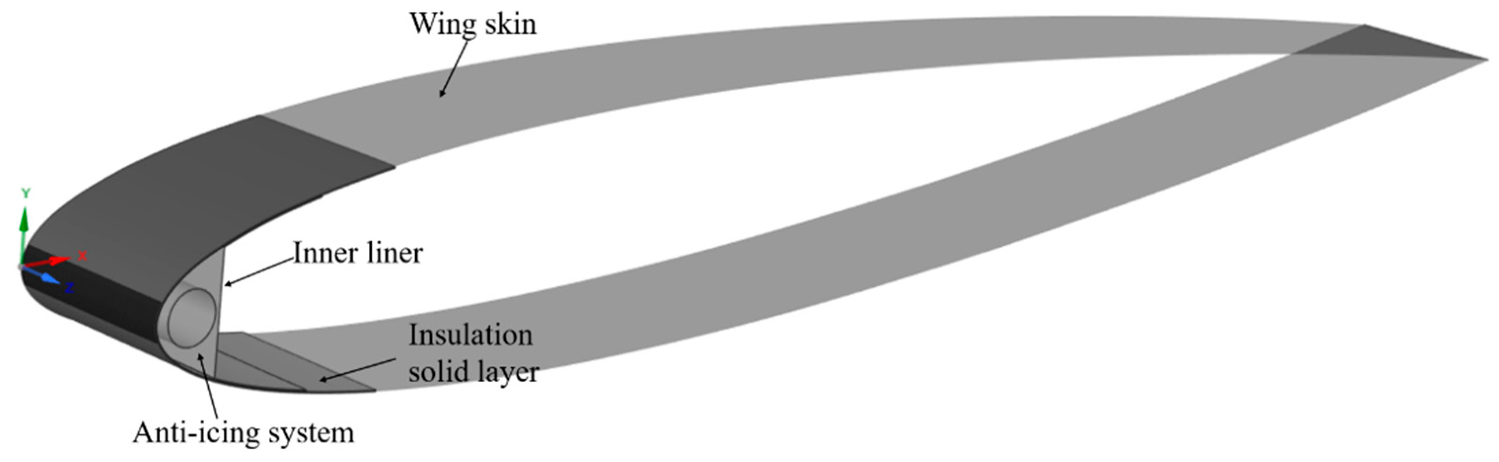
5. Piccolo Tube Hot Air Anti-Icing System

To ensure safe flight operations under icing conditions, effective airfoil anti-icing systems are essential for preventing ice accretion on aircraft surfaces. In this section, a hot air anti-icing chamber and an insulation solid layer are constructed within the interior of the NACA 0012 airfoil skin. Polynomial fitting models are applied to screen the external flow conditions for the CHT calculations. Finally, the effectiveness of this hot air anti-icing system is evaluated under severe icing conditions.

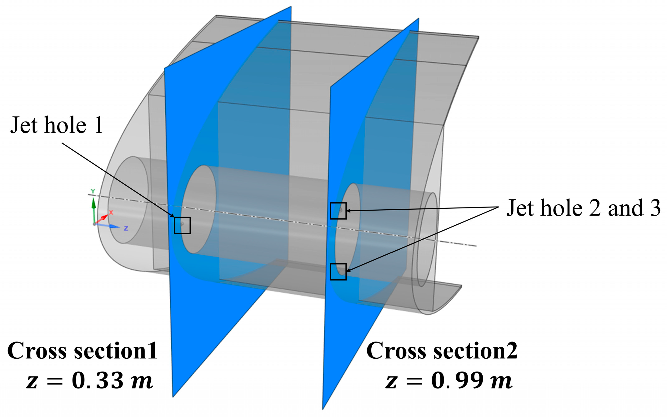
5.1. Numerical Calculation Models

An isometric view of the airfoil model with a hot air anti-icing system is shown in Figure 9. The detailed modeling and mesh generation results are provided in Appendix C.

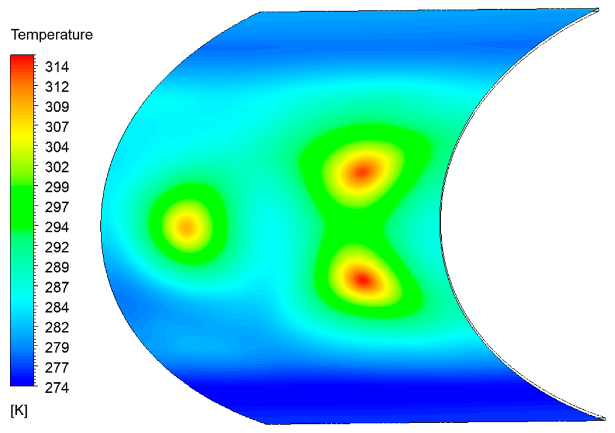
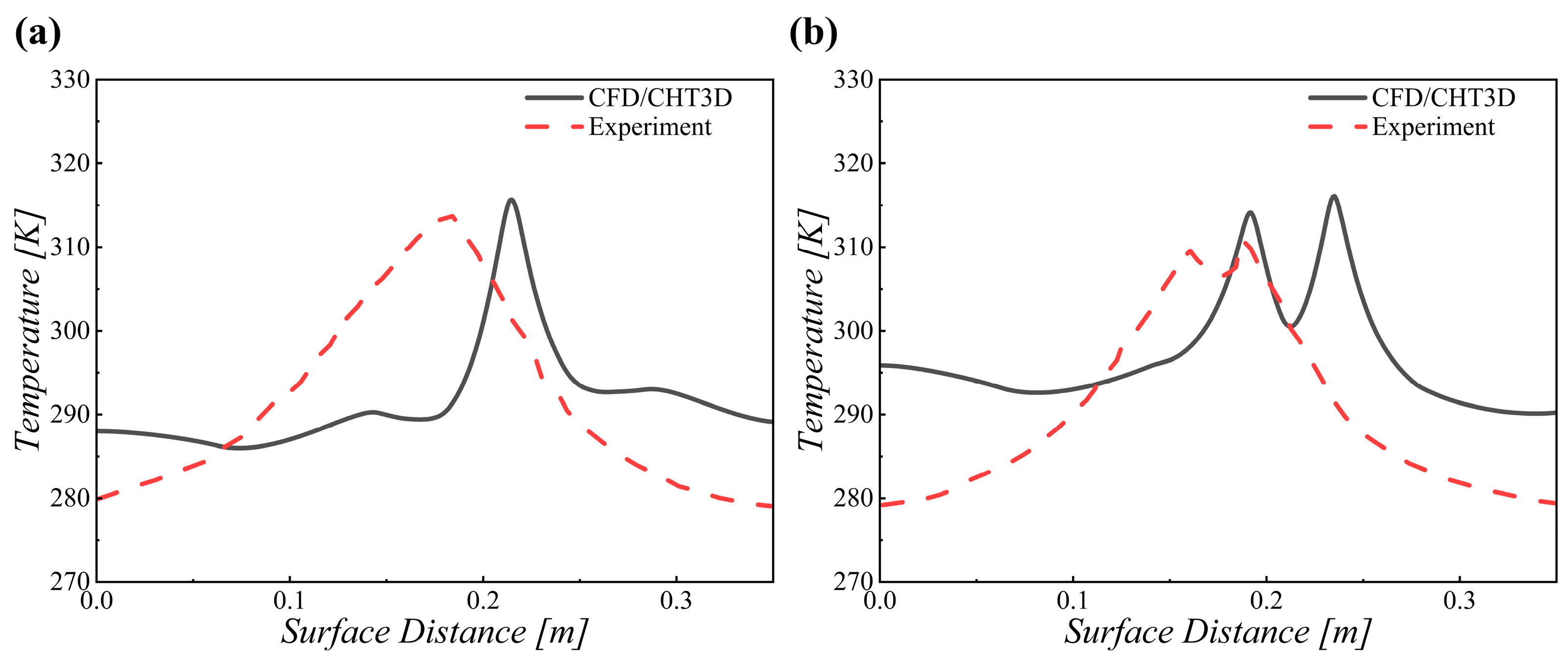
5.2. Validation of the Test Case

The anti-icing system was solved numerically via the CHT method. The CHT technique was applied to obtain three physical domains: the external airflow domain comprising the gas phase, the internal flow domain with hot air jets, and the thermal conduction in the airfoil skin from the interior surface of the airfoil leading edge to the runback flow on the external surface of the airfoil. Because hot and cold flows are computed separately in FLUENT and FENSAP-ICE, certain initial boundary conditions must be imposed to obtain the wall heat fluxes needed by the CHT3D module. The inlet to the external flow field is the same as that to the far pressure field in the previous icing calculations. For the internal flow, the jet holes are defined as mass flow inlets with a temperature of 449.817 K and a mass flow rate of 0.327 g/s. As indicated in

Table 5. Calculation conditions for the NASA IRT tests.

	Parameter	Unit	Value
Flight conditions	${\mathrm{V}}_{\mathrm{\infty }}$	m/s	59.2
	AOA	°	3
	${\mathrm{T}}_0$	K (°C)	268.21 (−4.94)
Icing conditions	MVD	μm	29
	LWC	g/m3	0.87
	Time	min	22.5
Hot air conditions	${\dot{m}}_{jet}$	g/s	0.327
	${\mathrm{T}}_{\mathrm{t}\mathrm{o}\mathrm{t},\mathrm{h}\mathrm{o}\mathrm{t}}$	K	449.817

, internal and external flow boundary conditions were adopted from NASA Icing Research Tunnel (IRT) tests [43,44,45].

Figure 10 shows the temperature contour map on the outer surface of the airfoil skin under the conditions listed in Table 5. The maximum temperature reached at the airfoil skin is 314 K, which occurs at the stagnation point of +45° for jet 2, and the minimum temperature of 274 K occurs at the end of the protection area of the lower skin surface. This finding indicates that the anti-icing system effectively maintains the airfoil’s surface temperature above freezing conditions under the given external conditions.

As shown in Figure 11, two cross sections were selected to determine the parameters for the analyses. Cross section 1 was set along the centerline of hot air jet 1 at $z=0.33 m$, whereas cross section 2 was set along the centerline of hot air jets 2 and 3 at $z=0.99 m$.

Figure 12 shows a comparison of the temperature distributions from CHT3D with Papadakis’s icing tunnel experimental data [44] at the two experimental cross sections, showing the temperatures extracted from the airfoil leading edge and the insulation solid outer surface. As shown in Figure 12a,b, the maximum temperature occurs in the jet stagnation area on the airfoil wall. The maximum temperatures obtained from the CHT3D simulations for cross sections 1 and 2 are slightly higher than the experimental values, with differences of 1.99 °C and 5.41 °C, respectively. Compared with the NACA 0012 symmetrical airfoil in this study, owing to the asymmetry of the model used in the NASA IRT experiments of the upper and lower surfaces, the temperature curves at the same cross-sectional locations are shifted to the left, with the shift in the peak temperature corresponding to the offset in the airfoil’s centerline.

Overall, the increases and decreases in the temperature distributions agreed with the experimental results. The average temperature error between the calculated and experimental results was less than 5%, with maximum temperature errors of 0.63% for cross section 1 and 1.76% for cross section 2. Therefore, the hot air anti-icing system used in this simulation is valid and can be used in subsequent analytical studies.

5.3. Validation of the Effectiveness of the Anti-Icing System Under Severe Icing Conditions

5.3.1. Severe Icing Conditions

Aircraft typically encounter severe icing conditions during flight. Evaluating the effectiveness of airfoil anti-icing systems under these severe conditions is essential for validating designs. The heat source of the hot air anti-icing system is bled from the high-pressure compressor of the jet engine to heat the wing surface, thereby preventing it from icing [46]. Therefore, higher heat loads are needed to increase the surface temperature of the wing above freezing at lower ambient temperatures. Additionally, ice thickness is a significant indicator of the severity of icing behavior. Higher thermal energy is needed to prevent icing under the icing conditions associated with a thicker ice layer.

Therefore, the most severe icing conditions include the lowest ambient temperature and thickest ice. The icing conditions corresponding to the minimum ambient temperature for each flight phase were selected from Table 3. Since direct measurements of maximum ice thicknesses for each phase were not available, maximum ice thickness polynomial models were used to estimate these extreme values.

Table 6. Severe icing conditions during all flight phases.

Flight Phase	Case	H (ft)	V∞ (m/s)	T0 (°C)	$\mathbf{M}\mathbf{V}\mathbf{D}$ (μm)	$\mathbf{L}\mathbf{W}\mathbf{C}$ (g/m3)	$\mathbf{T}\mathbf{i}\mathbf{m}\mathbf{e}$ (s)
Takeoff	1	1500	125 (243 kt)	−10	17.3	0.5137	258
	2	0		−30	15	0.2
	3	750		−30	15	0.2
	4	1500		−30	15	0.2
Climbing below 10,000 ft	5	10,000	128.6 (250 kt)	−8.30	20.66	0.4453	250
	6	1500		−30	15	0.2
	7	5500		−30	15	0.2
	8	9500		−30	15	0.2
Climbing above 10,000 ft	9	14,478	154.3 (300 kt)	−10	17.85	0.4948	210
	10	12,000		−30	15	0.2
	11	16,000		−30	15	0.2
	12	20,000		−30	15	0.2
Holding	13	13,344	136.3 (265 kt)	−2.69	21.85	0.5294	2700
	14	12,000		−30	15	0.2
	15	17,000		−30	15	0.2
	16	22,000		−30	15	0.2
Approach and landing	17	10,000	123.5 (240 kt)	−7.34	21.89	0.4322	260
	18	2000		−30	15	0.2
	19	6000		−30	15	0.2
	20	10,000		−30	15	0.2

presents the severe icing conditions for all the flight phases. Cases 1, 5, 9, 13, and 17 represent the icing conditions with the maximum ice thickness, and the other cases represent the icing conditions with the minimum ambient temperatures.

5.3.2. Calculation Results and Discussion

Figure 13 shows comparisons of the ice shapes under severe icing conditions without heating and runback ice after heating during the climbing phase above 10,000 ft, where the aircraft operates at a relatively high speed. Under the icing conditions without heating, at higher ambient temperatures, such as −10 °C, ice accretion extends above the horizontal axis (y = 0) even at an AOA of 8°, covering the upper surface of the airfoil, as indicated by the blue ice shape curves in Figure 13a. This phenomenon can be attributed to the higher LWC and the tendency of droplets to flow rearward along the airfoil surface under warmer conditions. In contrast, at a lower ambient temperature of −30 °C, as shown in Figure 13b–d, ice accretion primarily remains below the y = 0 axis and is confined to the lower surface of the airfoil.

When the hot air anti-icing system is activated, the red ice shape curves in Figure 13a–d represent the runback ice distribution calculated after the CHT simulation. At −10 °C (Figure 13a), which corresponds to the icing conditions associated with the maximum ice thickness, an irregular runback ice distribution emerges on the upper surface. This distribution is similar to the ice shape observed in icing tunnel experiments [45], with a maximum ice thickness of 9.89 mm.

At a lower ambient temperature of −30 °C, the ice distribution is also influenced by altitude. As shown in Figure 13b, at 12,000 ft, runback ice accretion occurs on both the upper and lower surfaces of the airfoil, with a maximum ice thickness of 2.44 mm obtained on the upper surface. However, at higher altitudes of 16,000 and 20,000 ft, as shown in Figure 13c,d, respectively, runback ice forms exclusively on the lower surface with smooth and hornless ice shapes, and the maximum ice thicknesses at these altitudes are 1.33 and 1.31 mm, respectively.

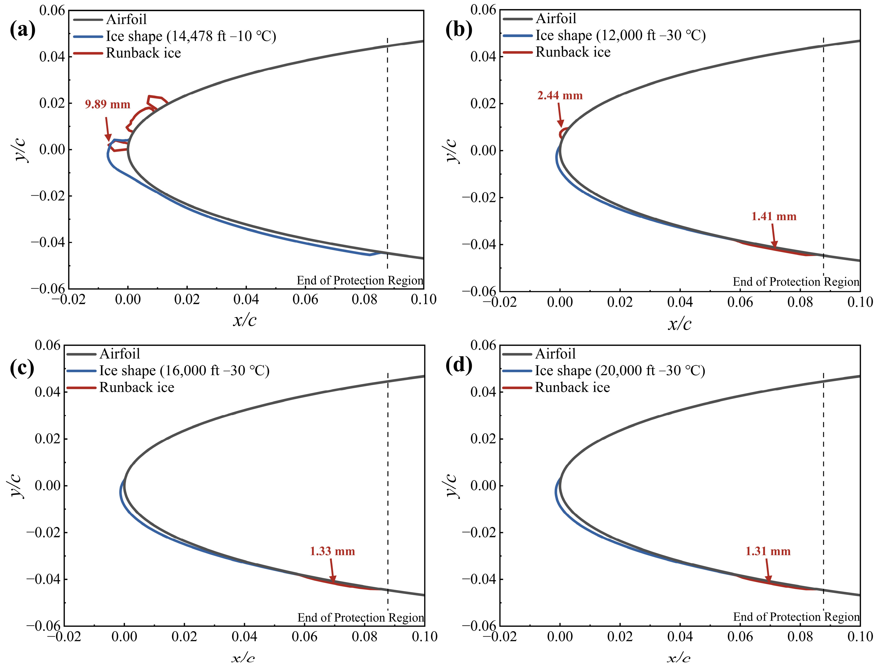
5.3.3. Analysis of the Effectiveness of the Anti-Icing System

The total ice mass under both unheated and heated conditions, along with the maximum runback ice thickness, are listed in

Table 7. Anti-icing efficiency under maximum icing thickness severe conditions.

Flight Phase	Case	Unheated Ice Mass (10−2 kg)	Heated Ice Mass (10−2 kg)	Anti-Icing Efficiency	Maximum Ice Thickness (mm)
Takeoff	1	5.23	0	100%	0
	2	1.6	0.573	64.19%	5.11
	3	1.62	0.579	64.26%	4.32
	4	1.65	0.587	64.42%	4.39
Climbing below 10,000 ft	5	6.9	0	100%	0
	6	1.67	0.631	62.22%	3.08
	7	1.8	0.64	64.44%	2.42
	8	1.94	0.665	65.72%	1.78
Climbing above 10,000 ft	9	6.84	1.78	73.98%	9.89
	10	2.2	0.73	66.82%	2.44
	11	2.35	0.527	77.57%	1.33
	12	2.52	0.544	78.41%	1.31
Holding	13	104.96	0	100%	0
	14	23.84	8.49	64.39%	17.07
	15	25.99	8.41	67.64%	16.51
	16	28.19	8.01	71.59%	16.09
Approach and landing	17	7.14	0	100%	0
	18	1.64	0.579	64.70%	4.38
	19	1.77	0.614	65.31%	2.12
	20	1.91	0.635	66.75%	1.73

. The critical ice thickness of 5 mm is considered the threshold for severe icing, with values above this threshold indicating a flight security risk. To evaluate the overall anti-icing performance of the system, the anti-icing efficiency was examined, which can be calculated as:

$$\begin{array}{c}Efficiency=\left|{\displaystyle \frac{m_u-m_h}{m_u}}\right|\times 100\%\end{array}$$

(2)

where $m_u$ and $m_h$ denote the total ice masses under unheated and heated conditions, respectively. As indicated in Table 7, the hot air anti-icing system provides effective protection against icing at ambient temperatures above −10 °C (thickest ice conditions), with 100% anti-icing efficiency achieved in four of the five flight phases and lower efficiency during the climbing phase above 10,000 ft (case 9). During this higher-altitude climbing phase, the increased airspeed results in greater convective heat losses, thereby requiring a higher thermal energy input to effectively prevent ice accretion [47]. However, the current internal flow conditions of the hot air anti-icing system do not meet the requirements for complete anti-icing under these conditions, leading to the removal of 73.98% of the accumulated ice, and the maximum runback ice thickness reaches 9.98 mm. This thickness of runback ice indicates that there may still be a risk of ice accretion even when the anti-icing system is activated.

At a lower ambient temperature of −30 °C (lowest temperature conditions), the hot air anti-icing system provides varying degrees of effectiveness, with the lowest anti-icing efficiency of 62.22% during the climbing phase below 10,000 ft (case 6) and the highest efficiency of 78.41% during the climbing phase above 10,000 ft (case 12). The maximum runback ice thicknesses in these two cases are 3.08 and 1.31 mm, respectively. Notably, during the takeoff phase (case 2), the maximum runback ice thickness reaches 5.11 mm, indicating anti-icing risk under these conditions.

In addition to cases 2 and 9, the extended exposure time during the 45 min (2700 s) holding phase led to significantly greater ice accretion in terms of both the ice thickness and mass. During this phase, the maximum runback ice thickness exceeded the critical 5 mm threshold for severe ice accretion, with values of 17.07, 16.51, and 16.09 mm for cases 14, 15, and 16, respectively. This highlights the importance of minimizing the exposure time or enhancing the performance of anti-icing systems during long-duration holding phases to prevent excessive ice accretion.

6. Conclusions

In this study, a rapid prediction method for the maximum ice thickness on an airfoil under various icing conditions was developed utilizing CFD simulations and polynomial regression model fitting. The most severe icing conditions for external flow were calculated based on the fitted models, and the effectiveness of the proposed anti-icing system was verified. First, the icing simulation results were compared with the icing tunnel test data to validate the feasibility of the established icing model. Icing meteorological conditions and flight conditions were derived from FAR part 25 Appendix C, flight manuals, and ICAO documents. Next, polynomial regression models were applied to the icing results, yielding 15 polynomial models for five flight phases and three ice types. These models were validated based on a test set to assess their prediction accuracy. Finally, a model of the airfoil’s internal hot air anti-icing system was established. The external flow conditions, calculated using the polynomial models, were used to evaluate the anti-icing performance of the system under the most severe icing conditions. The main conclusions are as follows:

(1)

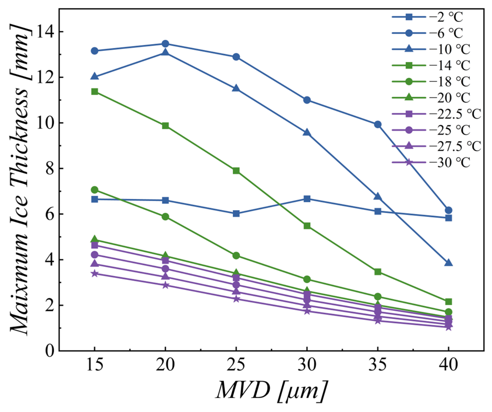
Under a constant external airspeed and AOA, the ice shape and maximum thickness are influenced by the temperature, MVD, and LWC. The temperature primarily affects the ice shape, the MVD mainly influences the icing area, and the LWC largely influences the ice thickness. With decreasing temperature, the ice shape transitions from angular glaze ice to rime ice with a smooth surface. The icing area and thickness under glaze ice conditions are affected by both the MVD and LWC. At a temperature of −2 °C, the maximum icing area occurs at an MVD of 20 μm, and the ice thicknesses under different MVD values vary between 6 and 7 mm. At temperatures of −6 °C and −10 °C, the maximum ice thickness occurs at an MVD of 20 μm. At other temperatures, as the MVD increases, the icing area gradually increases. An increase in the MVD is associated with a decrease in the LWC, leading to a decrease in the maximum icing thickness.

(2)

The icing results were classified into five flight phases (takeoff, climbing below 10,000 ft, climbing above 10,000 ft, holding, and approach/landing) and three ice types (glaze ice, mixed ice, and rime ice), resulting in a total of 15 datasets. Each icing calculation was treated as an isolated event. A quadratic polynomial regression model was applied to fit 80% of the data, with the remaining 20% reserved for testing. The test results demonstrated the high accuracy of the model, with the average relative error remaining below 3%. By inputting the icing condition parameters, these models provide rapid predictions of maximum ice thickness within an acceptable error margin compared with CFD calculations.

(3)

The anti-icing performance was validated by calculating the anti-icing capability of the proposed system under the most severe external flow icing conditions. An internal hot air anti-icing system incorporating a piccolo tube structure under the airfoil skin was modeled. The most severe icing conditions occurred when the ambient temperature was lowest and the ice was thickest, with the latter conditions derived from the prediction models. The hot air anti-icing system performed effectively under most icing conditions, particularly at temperatures above −10 °C. However, at a high climbing speed of 154.3 m/s during specific phases such as the takeoff phase and prolonged exposure during the holding phase, the system may face challenges in maintaining effective anti-icing performance, resulting in runback ice with a maximum thickness exceeding 5 mm.

References

1. Gent, R.W.; Dart, N.P.; Cansdale, J.T. Aircraft icing. Phil. Trans. R. Soc. A 2000, 358, 2873–2911. [Google Scholar] [CrossRef]
2. Bragg, M.B.; Broeren, A.P.; Blumenthal, L.A. Iced-airfoil aerodynamics. Prog. Aerosp. Sci. 2005, 41, 323–362. [Google Scholar] [CrossRef]
3. Lampton, A.; Valasek, J. Prediction of icing effects on the lateral/directional stability and control of light airplanes. Aerosp. Sci. Technol. 2012, 23, 305–311. [Google Scholar] [CrossRef]
4. Xie, L.; Liang, H.; Zong, H.; Liu, X.; Li, Y. Multipurpose distributed dielectric-barrier-discharge plasma actuation: Icing sensing, anti-icing, and flow control in one. Phys. Fluids 2022, 34, 071701. [Google Scholar] [CrossRef]
5. Su, Q.; Chang, S.; Song, M.; Zhao, Y.; Dang, C. An experimental study on the heat transfer performance of a loop heat pipe system with ethanol-water mixture as working fluid for aircraft anti-icing. Int. J. Heat Mass Transf. 2019, 139, 280–292. [Google Scholar] [CrossRef]
6. Dong, W.; Zheng, M.; Zhu, J.; Lei, G.; Zhao, Q. Experimental investigation on anti-icing performance of an engine inlet strut. J. Propuls. Power 2017, 33, 379–386. [Google Scholar] [CrossRef]
7. Cao, Y.; Ma, C.; Zhang, Q.; Sheridan, J. Numerical simulation of ice accretions on an aircraft wing. Aerosp. Sci. Technol. 2012, 23, 296–304. [Google Scholar] [CrossRef]
8. Janjua, Z.A.; Turnbull, B.; Hibberd, S.; Choi, K. Mixed ice accretion on aircraft wings. Phys. Fluids 2018, 30, 270101. [Google Scholar] [CrossRef]
9. Addy, H.E.; Potapczuk, M.G., Jr.; Sheldon, D.W. Modern airfoil ice accretions. In Proceedings of the 35th Aerospace Sciences Meeting and Exhibit, Reno, NV, USA, 6–9 January 1997. AIAA Paper 97-0174. [Google Scholar] [CrossRef]
10. Shin, J.; Bond, T.H. Results of an icing test on a NACA 0012 airfoil in the NASA Lewis icing research tunnel. In Proceedings of the 30th AIAA Aerospace Sciences Meeting and Exhibit, Reno, NV, USA, 6–9 January 1992; p. 647. [Google Scholar] [CrossRef]
11. Bowden, D.T.; Gensemer, A.G.; Sheen, C.A. Engineering Summary of Airframe Icing Technical Data; FAA Technical Report ADS-4; Federal Aviation Administration: Washington, DC, USA, 1963.
12. Messinger, B.L. Equilibrium temperature of an unheated icing surface as a function of air speed. J. Aeronaut. Sci. 1953, 20, 29–42. [Google Scholar] [CrossRef]
13. Myers, T.G. Extension to the Messinger model for aircraft icing. AIAA J. 2001, 39, 211–218. [Google Scholar] [CrossRef]
14. Hedde, T.; Guffond, D. ONERA three-dimensional icing model. AIAA J. 1995, 33, 1038–1045. [Google Scholar] [CrossRef]
15. Szilder, K.; Lozowski, E.P. Simulation of airfoil icing with a novel morphogenetic model. J. Aerosp. Eng. 2005, 18, 102–110. [Google Scholar] [CrossRef]
16. Prince Raj, L.; Lee, J.W.; Myong, R.S. Ice accretion and aerodynamic effects on a multi-element airfoil under SLD icing conditions. Aerosp. Sci. Technol. 2019, 85, 320–333. [Google Scholar] [CrossRef]
17. Lynch, F.T.; Khodadoust, A. Effects of ice accretion on aircraft aerodynamics. Prog. Aerosp. Sci. 2001, 37, 669–767. [Google Scholar] [CrossRef]
18. Miranda, L.R.; Elliott, R.D.; Baker, W.M. A Generalized Vortex Lattice Method for Subsonic and Supersonic Flow Applications; NASA Contractor Report 2865; NASA: Washington, DC, USA, 1977.
19. Erickson, L.L. Panel Methods: An Introduction; NASA Technical Paper 2995; NASA: Washington, DC, USA, 1990.
20. Boelens, O.J. CFD analysis of the flow around the X-31 aircraft at high angle of attack. Aerosp. Sci. Technol. 2012, 20, 38–51. [Google Scholar] [CrossRef]
21. Durst, F.; Miloievic, D.; Schönung, B. Eulerian and Lagrangian predictions of particulate two-phase flows: A numerical study. Appl. Math. Model. 1984, 8, 101–115. [Google Scholar] [CrossRef]
22. Ghenai, C.; Lin, C.X. Verification and validation of NASA LEWICE 2.2 icing software code. J. Aircr. 2006, 43, 1253–1258. [Google Scholar] [CrossRef]
23. Trontin, P.; Kontogiannis, A.; Blanchard, G.; Villedieu, P. Description and assessment of the new ONERA 2D icing suite IGLOO2D. In Proceedings of the 9th AIAA Atmospheric and Space Environments Conference, Denver, CO, USA, 5–9 June 2017; p. 3417. [Google Scholar] [CrossRef]
24. Aliaga, C.N.; Aubé, M.S.; Baruzzi, G.S.; Habashi, W.G. FENSAP-ICE-Unsteady: Unified in-flight icing simulation methodology for aircraft, rotorcraft, and jet engines. J. Aircr. 2011, 48, 119–126. [Google Scholar] [CrossRef]
25. Fossati, M.; Habashi, W.G. Multiparameter analysis of aero-icing problems using proper orthogonal decomposition and multidimensional interpolation. AIAA J. 2013, 51, 946–960. [Google Scholar] [CrossRef]
26. Xia, Y.; Li, T.; Wang, Q.; Yue, J.; Peng, B.; Yi, X. A rapid prediction method for water droplet collection coefficients of multiple airfoils based on incremental learning and multi-modal dynamic fusion. Phys. Fluids 2024, 36, 103313. [Google Scholar] [CrossRef]
27. Strijhak, S.; Ryazanov, D.; Koshelev, K.; Ivanov, A. Neural network prediction for ice shapes on airfoils using icefoam simulations. Aerospace 2022, 9, 96. [Google Scholar] [CrossRef]
28. Federal Aviation Administration. Part 25-Airworthiness Standards: Transport Category Airplanes; Federal Aviation Regulations; Federal Aviation Administration: Washington, DC, USA, 2013.
29. Massegur, D.; Clifford, D.; Da Ronch, A.; Lombardi, R.; Panzeri, M. Low-dimensional models for aerofoil icing predictions. Aerospace 2023, 10, 444. [Google Scholar] [CrossRef]
30. Li, S.; Qin, J.; He, M.; Paoli, R. Fast evaluation of aircraft icing severity using machine learning based on XGBoost. Aerospace 2020, 7, 36. [Google Scholar] [CrossRef]
31. Yang, Q.; Zheng, H.; Guo, X.; Dong, W. Experimental validation and tightly coupled numerical simulation of hot air anti-icing system based on an extended mass and heat transfer model. Int. J. Heat Mass Transf. 2023, 217, 124645. [Google Scholar] [CrossRef]
32. Silva, G.; Silvares, O.; Zerbini, E. Airfoil anti-ice system modeling and simulation. In Proceedings of the 41st AIAA Aerospace Sciences Meeting and Exhibit, Reno, NV, USA, 6–9 January 2003; p. 734. [Google Scholar] [CrossRef]
33. Yang, Q.; Guo, X.; Zheng, H.; Dong, W. Single-and multi-objective optimization of an aircraft hot-air anti-icing system based on Reduced Order Method. Appl. Therm. Eng. 2023, 219, 119543. [Google Scholar] [CrossRef]
34. Abdelghany, E.S.; Farghaly, M.B.; Almalki, M.M.; Sarhan, H.H.; Essa, M.E.-S.M. Machine Learning and IoT Trends for Intelligent Prediction of Aircraft Wing Anti-Icing System Temperature. Aerospace 2023, 10, 676. [Google Scholar] [CrossRef]
35. Lee, J.; Jo, H.; Choe, H.; Lee, D.; Jeong, H.; Lee, H.; Kweon, J.; Lee, H.; Myong, R.S.; Nam, Y. Electro-thermal heating element with a nickel-plated carbon fabric for the leading edge of a wing-shaped composite application. Compos. Struct. 2022, 289, 115510. [Google Scholar] [CrossRef]
36. Jung, S.K.; Prince Raj, L.; Rahimi, A.; Jeong, H.; Myong, R.S. Performance evaluation of electrothermal anti-icing systems for a rotorcraft engine air intake using a meta model. Aerosp. Sci. Technol. 2020, 106, 106174. [Google Scholar] [CrossRef]
37. Shin, J.; Bond, T.H. Experimental and Computational Ice Shapes and Resulting Drag Increase for a NACA 0012 Airfoil; National Aeronautics and Space Administration: Washington, DC, USA, 1992.
38. Fortin, G.; Ilinca, A.; Laforte, J.L.; Brandi, V. Prediction of 2D airfoil ice accretion by bisection method and by rivulets and beads modeling. In Proceedings of the 41st AIAA Aerospace Sciences Meeting and Exhibit, Reno, NV, USA, 6–9 January 2003; p. 1076. [Google Scholar] [CrossRef]
39. Airbus Customer Services. Getting to Grips with Aircraft Performance; Flight Operations Support & Line Assistance; Airbus S.A.S.: Toulouse, France, 2002. [Google Scholar]
40. International Civil Aviation Organization. 8168 OPS/611 Aircraft Operations: Procedures for Air Navigation Services-Volume II Construction of Visual and Instrument Flight Procedures; ICAO: Montréal, QC, Canada, 2006. [Google Scholar]
41. Cao, Y.; Tan, W.; Wu, Z. Aircraft icing: An ongoing threat to aviation safety. Aerosp. Sci. Technol. 2018, 75, 353–385. [Google Scholar] [CrossRef]
42. Cao, Y.; Yuan, K.; Li, G. Effects of ice geometry on airfoil performance using neural networks prediction. Aircr. Eng. Aerosp. Technol. 2011, 83, 266–274. [Google Scholar] [CrossRef]
43. Wright, W. An evaluation of jet impingement heat transfer correlations for piccolo tube application. In Proceedings of the 42nd AIAA Aerospace Sciences Meeting and Exhibit, Reno, NV, USA, 5–8 January 2004; p. 62. [Google Scholar] [CrossRef]
44. Hannat, R.; Morency, F. Numerical validation of conjugate heat transfer method for anti-/de-icing piccolo system. J. Aircr. 2014, 51, 104–116. [Google Scholar] [CrossRef]
45. Papadakis, M.; Wong, S.H.; Yeong, H.W.; Wong, S.C.; Vu, G. Icing tunnel experiments with a hot air anti-icing system. In Proceedings of the 46th AIAA Aerospace Sciences Meeting and Exhibit, Reno, NV, USA, 7–10 January 2008; p. 444. [Google Scholar] [CrossRef]
46. Guo, Z.; Zheng, M.; Yang, Q.; Guo, X.; Dong, W. Effects of flow parameters on thermal performance of an inner-liner anti-icing system with jets impingement heat transfer. Chin. J. Aeronaut. 2021, 34, 119–132. [Google Scholar] [CrossRef]
47. Liu, S.; Zhang, J. Influence of environment parameters on anti-icing heat load for aircraft. J. Aerosp. Power 2021, 36, 8–14. [Google Scholar] [CrossRef]
48. Mısır, O.; Akar, M. Efficiency and core loss map estimation with machine learning based multivariate polynomial regression model. Mathematics 2022, 10, 3691. [Google Scholar] [CrossRef]
49. Chicco, D.; Warrens, M.J.; Jurman, G. The coefficient of determination R-squared is more informative than SMAPE, MAE, MAPE, MSE and RMSE in regression analysis evaluation. PeerJ Comput. Sci. 2021, 7, e623. [Google Scholar] [CrossRef]
50. Chen, N.; Ji, H.; Cao, G.; Hu, Y. A three-dimensional mathematical model for simulating ice accretion on helicopter rotors. Phys. Fluids 2018, 30, 083602. [Google Scholar] [CrossRef]
51. Nwachukwu, A.; Jeong, H.; Pyrcz, M.; Lake, L.W. Fast evaluation of well placements in heterogeneous reservoir models using machine learning. J. Petrol. Sci. Eng. 2018, 163, 463–475. [Google Scholar] [CrossRef]
52. Zhang, W.; Wu, C.; Zhang, H.; Li, Y.; Wang, L. Prediction of undrained shear strength using extreme gradient boosting and random forest based on Bayesian optimization. Geosci. Front. 2021, 12, 469–477. [Google Scholar] [CrossRef]
Figure 1. Multistep icing calculation processes.
Aerospace 12 00492 g001
Figure 2. Computational grid for the NACA 0012 airfoil.
Aerospace 12 00492 g002
Figure 3. Comparison of the ice shapes under different conditions. (a) Multistep approach results for Case 1; (b) comparison of approaches with 1, 3, and 6 steps for Case 1; (c) multistep approach results for Case 2; (d) comparison of approaches with 1, 3, and 7 steps for Case 2.
Aerospace 12 00492 g003
Figure 4. Continuous maximum icing envelope, adapted from Ref. [28]. (a) Continuous maximum icing envelope (LWC vs. MVD); (b) continuous maximum icing envelope (temperature vs. altitude).
Aerospace 12 00492 g004
Figure 5. Influence of airspeed and AOA on the maximum ice thickness. (a) Influence of airspeed on glaze ice (−10 °C), mixed ice (−15 °C), and rime ice (−25 °C); (b) influence of the AOA on glaze ice (−10 °C), mixed ice (−15 °C), and rime ice (−25 °C).
Aerospace 12 00492 g005
Figure 6. Simulated ice shapes under different conditions. (a) Glaze ice at 271.15 K (−2 °C), (b) glaze ice at 267.15 K (−6 °C), (c) glaze ice at 263.15 K (−10 °C), (d) mixed ice at 259.15 K (−14 °C), (e) rime ice at 253.15 K (−20 °C), and (f) rime ice at 243.15 K (−30 °C).
Aerospace 12 00492 g006
Figure 7. Maximum ice thickness under different icing conditions.
Aerospace 12 00492 g007
Figure 8. True maximum ice thickness values versus predicted values. (a) Takeoff phase, (b) climbing phase below 10,000 ft, (c) climbing phase above 10,000 ft, (d) holding phase, and (e) approach and landing phase.
Aerospace 12 00492 g008
Figure 9. Airfoil model with a hot air anti-icing system.
Aerospace 12 00492 g009
Figure 10. Airfoil skin temperature contour map.
Aerospace 12 00492 g010
Figure 11. Selected cross sections along the airfoil chord direction.
Aerospace 12 00492 g011
Figure 12. Temperature distribution: warm and wet conditions. (a) Leading edge wall: cross section 1; (b) insulation solid surface: cross section 2.
Aerospace 12 00492 g012
Figure 13. Simulated ice shapes under severe freezing conditions. (a) Case 9, H = 14,478   f t , T 0 = 10   ° C , M V D = 17.85   μ m , L W C = 0.4948   g / m 3 ; (b) case 10, H = 12,000   f t , T 0 = 30   ° C , M V D = 15   μ m , L W C = 0.2   g / m 3 ; (c) case 11, H = 16,000   f t , T 0 = 30   ° C , M V D = 15   μ m , L W C = 0.2   g / m 3 ; (d) case 12, H = 20,000   f t , T 0 = 30   ° C , M V D = 15   μ m , L W C = 0.2   g / m 3 .
Aerospace 12 00492 g013