Article

Structural Parameter Optimization of the Vector Bracket in a Vertical Takeoff and Landing Unmanned Aerial Vehicle

1
School of Mechanical Engineering, Shaanxi University of Technology, Hanzhong 723001, China
2
School of Mechanics, Civil Engineering and Architecture, Northwestern Polytechnical University, Xi’an 710129, China
*
Author to whom correspondence should be addressed.
Aerospace 2025, 12(6), 487; https://doi.org/10.3390/aerospace12060487
Submission received: 24 April 2025 / Revised: 26 May 2025 / Accepted: 27 May 2025 / Published: 29 May 2025
(This article belongs to the Section Aeronautics)

Abstract

The functionality of unmanned aerial vehicles (UAVs) in agricultural applications was improved by optimizing the parameters of the vector bracket in a vertical takeoff and landing UAV to maximize thrust and lift-to-drag ratio. First, the results of computational fluid dynamics simulations were compared with wind tunnel data to ensure an accurate model of the considered UAV, indicating a thrust coefficient error of less than 3% and a UAV lift-to-drag ratio error of less than 8%. Next, this model was applied to simulate the propeller thrust and UAV lift-to-drag ratio for 25 sample points selected using a central composite experimental design by varying the four structural parameters of the vector bracket. A kriging algorithm was subsequently applied to construct response surface models based on the results. Finally, a Multi-Objective Genetic Algorithm was employed to determine the optimal parameter values maximizing the two coefficients. The optimal structural parameters for the UAV vector bracket were determined to comprise a vector bracket height of 51 mm, fixed bracket length of 168 mm, fixed bracket width of 69 mm, and ball socket outer diameter of 31 mm. These values provided a 19% larger propeller thrust coefficient than those of the original UAV.

1. Introduction

The advancement of precision farming technologies has facilitated the efficient gathering of vegetation data through drone-based remote sensing systems. “While conventional fixed-wing UAVs demonstrate superior cruise efficiency with high-speed horizontal flight capabilities and extended endurance, their operational effectiveness is constrained by inherent limitations in takeoff and landing control”. Conventional multirotor UAVs possess vertical takeoff and landing (VTOL) capabilities, yet demonstrate limited performance in sustained high-velocity horizontal flight operations with restricted endurance. Consequently, VTOL UAVs were developed to integrate the superior VTOL performance of multirotor platforms with the optimized aerodynamic efficiency characteristic of fixed-wing aircraft designs. The integrated methodology successfully tackled limitations related to restricted operational distance, suboptimal flight performance, and challenging launch/recovery procedures, thereby enabling extended mission durations while eliminating dependency on sophisticated auxiliary systems. Consequently, VTOL unmanned aerial vehicles present an effective solution for meeting the growing sophistication of near-surface agricultural monitoring applications [1,2,3,4,5].
Numerous research efforts have utilized computational fluid dynamics (CFD) techniques for enhancing the aerodynamic performance and structural configuration of VTOL UAVs. Li [6] enhanced the transitional flight phase performance for vertical takeoff and landing unmanned aerial vehicles, with computational fluid dynamics serving as the verification methodology. Li and Liu [7] performed systematic aerodynamic optimization of shrouded propulsion systems for vertical takeoff and landing unmanned aerial vehicles. Through careful selection of performance metrics for rotor characterization and implementation of evolutionary multi-criteria optimization techniques, the refined prototype demonstrated enhancements of 5.3% in overall pressure ratio and 7.8% in thermodynamic efficiency relative to the baseline configuration. Czyba [8] employed computational fluid dynamics to examine variations in aerodynamic efficiency (lift–drag ratio) across different operational phases—including vertical ascent/descent, transitional maneuvering, and level flight—for the purpose of refining both airfoil geometry specifications and propulsion system mounting configurations on a vertical takeoff and landing unmanned aerial vehicle. “Seong [9] conducted a systematic investigation of propeller-induced airflow modifications and their effects on wing aerodynamics at different orientations, quantifying the complex interactions between propulsion systems and airframe aerodynamics across multiple flight regimes”.
“Although computational fluid dynamics (CFD) has proven invaluable for aerodynamic simulation and structural optimization of UAVs, its reliance on discrete numerical outputs creates fundamental limitations in determining globally optimal design parameters”. This limitation has been addressed through the widespread use of response surface models (RSMs) and Multi-Objective Genetic Algorithms (MOGAs) to obtain global optimal solutions [10,11]. Shirazi [12] addressed the critical environmental issue of watershed soil erosion control by employing a response surface methodology to optimize soil physical properties and hydraulic parameters. The research results demonstrated a significant reduction in watershed soil erosion from 11.537 (pre-treatment) to −2.253 (post-optimization). Verma [13] and collaborators employed a response surface methodology to forecast peak hydrocarbon production in the catalytic thermochemical decomposition of heterogeneous plastic waste, achieving a minimal deviation of merely 0.19% relative to empirical data. Powar [14] employed a response surface methodology to investigate the influence mechanisms of three key parameters on threshing efficiency, milling efficiency, and grain breakage rate. The results indicated that, by developing a parameter optimization model, the optimal parameter combination was identified, achieving 99% threshing efficiency and 86% milling efficiency while maintaining a grain breakage rate at a remarkably low level of 0.1%. Eskandari [15] utilized a response surface methodology for machining parameter optimization, specifically targeting spindle rotation speed, material feed rate, tool advancement velocity, and cutting penetration depth, with the objectives of minimizing cutting resistance, reducing tool flank wear, and maximizing workpiece removal efficiency. Li [16] integrated a response surface methodology with an instructional optimization approach, establishing peak cutting resistance and minimal surface texture irregularity as dual optimization criteria for enhancing machining parameters including tool velocity, per-insert feed rate, longitudinal cut depth, and transverse engagement width. Post-optimization analysis revealed a 2.7% augmentation in cutting force coupled with a 6.63% improvement in surface finish quality and a 49.42% enhancement in stock removal productivity. Negemiya [17] implemented a hybrid approach integrating a response surface methodology and PSO (particle swarm optimization) to enhance the mechanical properties of Ti-alloyed austenitic stainless steel through precise adjustment of three key process variables: interfacial compression force, thermal treatment temperature, and dwell duration.
As a powerful optimization paradigm, evolutionary computation based on genetic principles offers significant advantages over conventional optimization approaches through its guided stochastic exploration mechanism for identifying globally optimal solutions in multidimensional problem spaces. Vishwanath [18] and collaborators employed a Box–Behnken design methodology to systematically investigate how key process variables—including the rotational velocity of the spindle, material advancement rate, and cutting tool engagement width—influence the surface finish quality in EN36 alloy steel turning operations. Through a response surface methodology, they formulated a predictive roughness model, with genetic optimization yielding an achieved surface texture refinement of 1.19 μm. Park [19] implemented a hybrid optimization strategy combining evolutionary computation and bio-inspired fish swarm intelligence, achieving a 35-fold acceleration in parameter optimization for tuned vibration absorbers compared to traditional global search methodologies. Zhu [20] integrated a response surface methodology with evolutionary computation techniques to determine the optimal wing configuration parameters—including airfoil quantity and structural spar placement—for unmanned aerial vehicles, achieving a 9.28% reduction in overall airframe mass. Mohammad [21] employed Taguchi’s experiment design with 25 sampling configurations to refine the airframe design of a fixed-wing unmanned aerial vehicle. A response surface model incorporating six key aerodynamic parameters influencing the lift-to-drag ratio was developed, with this ratio’s maximization serving as the primary optimization criterion during the evolutionary algorithm implementation. The final design iteration achieved a 55% enhancement in the vehicle’s aerodynamic efficiency, marking successful convergence of the optimization procedure.
VTOL-capable unmanned aerial systems accomplish flight mode conversions between vertical and cruising states through vectoring bracket angle modulation. Given the predominant operation in level flight regimes, this study primarily focused on optimizing the structural configuration of the vector bracket for improved cruising flight aerodynamics. Computational fluid dynamics analyses generated kriging-enhanced response surface models correlating bracket geometry variations with both propulsive thrust output and airframe aerodynamic performance metrics, followed by multi-objective evolutionary optimization targeting simultaneous maximization of these key parameters.

2. Materials and Methods

2.1. Structure of the Considered UAV

The vertical takeoff and landing unmanned aerial vehicle under investigation features a tailless flying-wing design with rear-mounted propulsion, shown schematically in Figure 1. Its airframe structure integrates symmetrically arranged main lifting surfaces incorporating tip-mounted vertical stabilizers coupled with a thrust-vectoring assembly that provides support for both the electric motor and its associated rotor. Longitudinal carbon-fiber spars extend continuously through the main wings and stabilizers to enhance structural rigidity, with the central fuselage section created through interconnection of the inboard wing sections. Specifically engineered for this application, the thrust-vectoring mechanism interfaces with the airframe at its proximal extremity while anchoring the propulsion unit distally. It comprises a fixed bracket, a ball joint bearing, a ball socket, universal joints, push rods, and a servo, and was considered to be in the horizontal flight condition.
As shown in Figure 2, the wing uses a Sipkill 1.7/10 airfoil with a reference area of 0.48 m2 and an aspect ratio of 3. Table 1 details the geometric dimensions of the wing in terms of the span b , root chord c r , tip chord c t , and sweep angle Λ w and those of the winglet in terms of the spanwise length at the tip l y s , height l v , sweep angle Λ v , thickness h , and support foot length l j c (the distance between the two supporting feet of the winglet).

2.2. Vector Bracket Manufacturing

The vector bracket designed in this study was fabricated using polylactic acid (PLA) material through 3D printing technology for integrated forming. PLA exhibits high specific strength and lightweight characteristics, which can satisfy the static load-bearing requirements of the UAV propeller and motor system. However, during long-term service under continuous loading, creep deformation may occur in the PLA material, leading to structural deformation of the vector bracket and consequently affecting the accuracy of the propeller’s thrust direction. In more severe cases, such continuous deformation may induce material fatigue, ultimately causing bracket fracture and endangering flight safety. Therefore, special attention should be paid to the long-term reliability of this structure in practical applications.

2.3. Range of Structural Parameters

According to the relevant literature [22,23,24,25], an increase in the area of the VTOL UAV tail region shields more incoming flow, resulting in a higher thrust coefficient for the pushing propeller. However, an increase in the area of the tail region also decreases the lift-to-drag ratio of the UAV, which is expressed using the lift-to-drag ratio. The tail section of the UAV considered in this study was equipped with a vector bracket to change the orientation of the propeller according to flight mode. Changing the structural parameters of this bracket, which are defined as the vector bracket height (H), fixed bracket length (L), fixed bracket width (W), and ball socket outer diameter (D), as shown in Figure 3, alters the area of the UAV tail region. Therefore, these parameters must be optimized to balance the propeller thrust and vehicle lift-to-drag ratio.
Changing H alters the aerodynamic interaction between the propeller and UAV; thus, determining an appropriate H is critical to ensuring that both the UAV and propeller exhibit optimal aerodynamic performance. Several researchers have conducted in-depth studies on the aerodynamic interference between UAVs and their propellers by exploring various propeller mounting distance ranges for the UAV and propeller. For instance, Zhang et al. examined a range of 0.24–0.64R, where R represents the propeller radius [22], Sun and Zhao analyzed a range of 30–190 mm [23], and Shi et al. investigated a range of 14–90 mm [24,25]. Furthermore, because the vector bracket provides the structural connection between the propeller and UAV, an excessive H might weaken the bracket strength and make it prone to deformation. Conversely, an insufficient H might make the flow field interaction between the UAV and propeller too intense. Therefore, this study evaluated H values at the 30 mm increments within 30–150 mm.
The fixed bracket has to have sufficient contact area with the fuselage to ensure its secure attachment to the UAV. Therefore, its minimum L and W were set to 30 mm. However, as an excessive L and W would increase the load-bearing area, leading to higher drag and reduced flight efficiency, the maximum L and W were set to 170 mm. Thus, L and W were varied using the 30 mm increments within 50–170 mm.
Finally, as the motor is mounted on the outside of the vector bracket ball socket, D has to be larger than the diameter motor. The motor considered in this study was the Long Yu X2814 KV100, which is specified to have an external diameter of 28 mm. Therefore, the minimum D was set using the 17.5 mm increments within 30–100 mm.
The ranges of the four vector bracket parameters are listed in Table 2.

2.4. Numerical Simulation Method

2.4.1. Fluid Control Equation

The air medium in the external flow field around the UAV was considered incompressible because this study focused on low-speed flight. The Navier–Stokes (N–S) equations comprise the most common flow model in fluid mechanics and represent the most comprehensive differential equations for describing incompressible fluids. The N–S equations reflect the fundamental laws of viscous fluid dynamics and are invaluable in fluid mechanics accordingly. These equations rely on differential equations to describe fluid motion. In contrast to algebraic equations, the N–S equations do not attempt to establish direct relationships between the variables under study but instead seek to describe the rates of change or fluxes of quantities. Owing to the nonlinear partial differential nature of the N–S equations, their solutions are highly complex and difficult to obtain, with accurate solutions only being achievable for certain simplified problems. However, the development of computer simulation technology has facilitated the numerical solution of these equations in many previously unsolvable scenarios.
Under the operational condition of the UAV at a flight speed of 20 m/s and 4° angle of attack, the Navier–Stokes equations, as the governing equations of fluid motion, accurately describe the flow field characteristics around the aircraft. Building upon this foundation, we employed the Spalart–Allmaras turbulence model to address complex turbulent phenomena in the flow field. This model effectively simulates turbulence features such as boundary layer separation and vortex development through its single-equation transport formulation. The computational results, coupled with the N–S equations, provide a theoretical basis for analyzing the thrust characteristics and lift-to-drag ratio performance of the UAV during cruise conditions. The three-dimensional incompressible N–S equations [26,27] are expressed as follows:
ρ D u D t = ρ f x p x + μ 2 u ρ D v D t = ρ f y p y + μ 2 ν ρ D w D t = ρ f z p z + μ 2 w
where u , v , and w represent the dimensionless velocity components along the x , y , and z directions, respectively; p and t denote the dimensionless pressure and time, respectively; ρ and μ are the fluid density and molecular kinematic viscosity coefficient, respectively; f x , f y , and f z represent the body force components per unit mass along the x , y , and z directions, respectively; is the Hamiltonian operator; and Δ is the Laplace operator.
By multiplying Equation (1) by the unit vectors i , j , and k in the three respective coordinate directions and summing the results, the simplified vector form of the N–S equations for an incompressible viscous fluid flow can be expressed as
D V D t = f 1 ρ p + μ ρ Δ V
where V = u i + v j + w k represents the velocity vector components, = x i + y j + z k , and Δ = 2 x 2 + 2 y 2 + 2 z 2 .

2.4.2. Turbulence Model

The Spalart–Allmaras (S-A) model [28] was selected for the UAV simulations primarily due to its computational efficiency and robustness, particularly for handling large-scale meshes (e.g., drone and propeller geometries). Under the operating condition with a freestream velocity of 20 m/s, this model effectively balances computational accuracy and efficiency requirements. Compared to more complex turbulence models (such as k-ε or k-ω), the S-A model only requires solving one transport equation, significantly reducing computational costs while maintaining sufficient accuracy for typical flow characteristics (including attached flows and mild flow separations) within the 20 m/s velocity range. Its numerical stability makes it suitable for aerodynamic simulations at this velocity condition, ensuring reliable convergence even with dense meshes. Therefore, for performance analysis of medium-speed UAVs in this category, the S-A model achieves an optimal balance between speed, stability, and accuracy. The governing transport equation for the S-A turbulence formulation is expressed as follows:
ρ d v ¯ d t = G v + 1 σ v ¯ { x j [ ( μ + ρ v ¯ ) v ¯ x j ] + C b 2 ρ [ v ¯ x j ] 2 } Y v
where G v is the turbulent pulsating viscosity, v ¯ is the kinematic viscosity coefficient for non-near-wall surfaces, σ v ¯ and Y v are constants to be determined, and C b 2 ρ is the turbulent viscous loss in the wall region.

2.4.3. Multiple Reference Frame Model

The multiple reference frame (MRF) model is widely used in CFD simulations and is particularly suitable for flow simulations involving rotating components such as propellers, turbines, or fans. The MRF model enables the simulation of relative motion in rotating machinery by defining stationary and rotating reference frames, obviating the need to simulate transient rotational processes. This approach reduces computational complexity and the associated costs. The computational domain in an MRF model is divided into multiple subdomains, each with its own independent reference frame. Typically, these frames are classified as stationary or rotating: the former is applied to fixed components, such as the static fluid region outside the propeller, where quantities such as velocity and pressure are described from the perspective of a fixed observer; the latter is applied to rotating components, such as the propeller, where quantities such as the velocity and pressure are described from the perspective of an observer rotating along with the rotating component [29].
This study used steady-state calculations to simulate the UAV and propeller during horizontal flight and applied the MRF model to simulate the rotors. As shown in Figure 4, the computational domain was divided into rotating and stationary regions for meshing accordingly. The region between the rotor and interface (indicated by the dashed line) was defined as the rotating domain, whereas the area outside the interface was defined as the stationary domain.

2.4.4. Flow Field Model and Meshing

The UAV simulation model was divided into dynamic and static domains to simulate the complex aerodynamic interactions between the propeller, surrounding fluid, and stationary components. The entire CFD flow field model was also divided into dynamic and static domains for computational processing accordingly. The flow field region of the propeller was modeled as a disk-shaped dynamic domain computed using a rotating coordinate system that shared the same rotational axis as the propeller. The UAV fuselage was located within a cylindrical static domain. The mesh nodes at the interface between the static and dynamic domains were made to coincide perfectly using a shared conformal topology that treated the interface as an internal face. This approach is more accurate than the conventional interface method as it effectively eliminates any error introduced by the need to use interpolation for information exchange between dynamic and static domains.
As shown in Figure 5, the height and diameter of the static domain were set to ten and five times the wingspan of the UAV model, respectively. The distance between the inlet of the static domain and leading edge of the UAV was four times the wingspan, and the distance between the outlet of the static domain and trailing edge of the UAV was six times the wingspan. The diameter of the dynamic domain was 100 mm larger than the rotational diameter of the propeller, and the distance between the propeller hub and dynamic domain surface was 15 mm in one direction and 85 mm in the other. A combination of hexahedral and polyhedral mesh types was employed to discretize the different regions of the flow field. Polyhedral meshes were used to model the leading and trailing edges of the UAV wings and propeller, whereas hexahedral meshes were employed to model the static and dynamic domains [30]. This approach simplified the computational process and enabled precise flow field simulations under various flow conditions, thereby improving the accuracy and efficiency of the overall simulation. Surface viscosity effects and the influence of the boundary layer on the UAV and propeller calculations were considered by adding prism boundary layers in the direction normal to the UAV and propeller surfaces to accommodate the steep velocity gradients within the boundary layer. The first-layer grid height was set to 0.07 mm for the UAV model and 0.01 mm for the propeller model based on actual conditions. The final mesh comprising the UAV and propeller had a skewness of 0.6 and an orthogonal quality of 0.2 with a total mesh count of 4,534,362.
The boundary conditions of the flow field were established as follows: the inlet was set as a velocity inlet with an incoming flow velocity of 20 m/s and the outlet was set as a standard atmospheric pressure; the angle of attack was varied from 4° to 12° in 2° increments; the boundaries of the computational domain were assumed to exhibit the no-slip condition; the near-wall treatment used the standard boundary equations, which were solved using the distributed SIMPEC algorithm; finally, the propeller wall was set as a rotating wall.

2.5. Optimization Approach

2.5.1. Structural Parameter Optimization Process

The optimization flow chart of the vector bracket is shown in Figure 6. First, a central composite design (CCD) was used to design the test scheme. Second, computational fluid dynamics (CFD) was employed to conduct sample point calculations. The calculation results were then imported into the Response Surface Module to construct a response surface model. Finally, a genetic algorithm was used to optimize the structural parameters.

2.5.2. Central Composite Experimental Design

As a sophisticated experimental design methodology, central composite design (CCD) utilizes a five-level fractional factorial framework specifically developed for quadratic response surface model calibration [31]. Within the CCD family, three principal variants exist for experimental program formulation: circumscribed (CCC), inscribed (CCI), and face-centered (CCF) configurations. The current research adopted the CCC approach. Geometrically represented in Figure 7, the coded variable space for each parameter spanned five distinct levels, denoted as ( β , 1 , 0 , + 1 , + β ) . Here, the ( 1 , + 1 ) interval is mapped to the experimentally defined parameter bounds, while the ( β , + β ) range extends these limits to establish augmented operational extremes for comprehensive factor space exploration.
The thrust characteristics and aerodynamic performance were primarily determined by four key geometric parameters (H, L, W, D). A central composite design methodology was employed to construct the experimental scheme for these four structural variables, comprising 16 factorial cube points, 8 axial star points, and 1 central reference point. Through computational fluid dynamics simulations, corresponding propulsion performance and aerodynamic characteristics were obtained at 25 optimized sampling points.

2.5.3. Kriging-Algorithm-Based RSMs

Response Surface Methodology (RSM)
We approximated the response values at non-tested points by utilizing experimental data as a substitute for complex models. Its core principle involved determining input and output variables, employing appropriate experimental design methods to obtain test data, and applying a multivariate quadratic regression equation to fit the mapping relationship between inputs and outputs. The response surface model exhibited excellent differentiability and continuity, simplified the optimization process, and was suitable for solving with conventional mathematical optimization methods.
As a spatial statistics-based interpolation technique, the kriging model not only effectively handles complex nonlinear problems but also fully utilizes the spatial correlation between sample points, demonstrating superior performance in prediction accuracy and model reliability. Compared with traditional polynomial models, kriging better captures the complex mapping relationship between design variables and target parameters, particularly excelling in prediction performance when sample data are limited.
Given these advantages, to further analyze the nonlinear relationship between the structural parameters of vector scaffolds and performance metrics, this study selected the kriging algorithm to construct the response surface model. The model established the relationship between the thrust coefficient, lift-to-drag ratio, and structural parameters.
The mathematical expression for the kriging algorithm [32] is given by
y x = f T x β + z x
where β represents the regression coefficient; f x denotes the polynomial of the design parameter x , serving as the global approximation model; and z ( x ) is a zero-mean random function used to approximate local deviations that exhibit the following statistical properties:
E z x = 0
Var [ z x ] = σ z 2
Cov [ Z ( x i ) , Z ( x j ) ] = σ 2 [ R i j ( θ , x i , x j ) ]
in which x i and x represent any two input variables, R i j ( θ , x i , x j ) is the correlation function with the parameter θ , and the stochastic process z ( x ) determines the accuracy of the model as follows:
R i j ( θ , x i , x j ) = exp k = 1 n m θ k | x k i x k j | 2
where n m represents the number of random variables; the k component corresponding to x i and x j is denoted as x k i and x k j , respectively; and θ k is the correlation parameter, which is determined using the maximum likelihood estimation of the correlation function given by
θ = min [ ( det R ) 1 m σ 2 ]
For a given input variable set X = x 1 , x 2 , , x n and its corresponding response set Y = y 1 , y 2 , , y n , the estimated values of β and σ 2 can be determined as follows:
β ^ = F T R 1 F 1 F T R 1 Y
σ ^ z 2 = 1 N 0 ( y β F ) T R 1 ( Y β F )
where N 0 represents the dimensionality of the vector.
Finally, the predicted response value for test point x obtained using the kriging algorithm is given by
y ^ x = β ^ + r T ( x ) R 1 ( Y f β ^ )
in which
f = f x 1 , f x 2 , , f x n T
r x = R x , x 1 , R x , x 2 , , R x , x n T
After the kriging algorithm was applied to construct the RSMs using the experimental design points and response values, it was applied to predict the coefficient response values at the test points.

2.6. MOGA Optimization

The Multi-Objective Genetic Algorithm (MOGA) is employed to simultaneously optimize multiple conflicting objectives through genetic operations including selection, crossover, and mutation. In the MOGA framework, solution quality is evaluated using the Pareto dominance relationship, where solution A is considered to dominate solution B if it is at least as good as B in all objectives and superior in at least one objective. The algorithm utilizes non-dominated sorting to classify solutions into different ranks and applies crowding distance to maintain population diversity, thereby preventing premature convergence to local optima. Ultimately, the MOGA generates a set of Pareto-optimal solutions representing balanced trade-offs among competing objectives. This approach has found widespread application in complex domains such as engineering design, path planning, and resource allocation.
For the structural optimization of vector brackets, which inherently involves the synthesis and evaluation of multiple conflicting design criteria, the MOGA methodology demonstrates particular advantages. Accordingly, the multi-objective optimization problem for vector brackets was formulated as the following mathematical model:
max K ( x ) = [ K 1 ( x ) , K 2 ( x ) , , K n ( x ) , ] maxC T ( x ) = [ C T 1 ( x ) , C T 2 ( x ) , , C T n ( x ) , ]
where K ( x ) denotes the lift-to-drag ratio of the UAV and C T ( x ) denotes the propeller thrust coefficient for structural parameter set x with the following constraints:
n = 1 , 2 , N K i ( x ) K 0 ( x ) C T j ( x ) C T 0 ( x ) x = [ x 1 , x 2 , , x d , , x D ] x d m i n x d x d m a x d = 1 , 2 , 3 , 4 i = 1 , 2 , , m ; j = 1 , 2 , , k
where m , n , i , j , d denote the number of variable states and x d denotes the considered range of the structural parameters.
(1) Flow of Genetic Algorithm
(1)
Initial Population of Multi-Objective Genetic Algorithm (MOGA)
The initial population is used to run the Multi-Objective Genetic Algorithm (MOGA).
(2)
MOGA Generates New Populations
The Multi-Objective Genetic Algorithm is executed to generate new populations through crossover and mutation. After the first iteration, each population is run when it reaches the number of samples defined by the “number of samples per iteration” attribute.
(3)
Design Point Update
The design points are updated in the new population.
(4)
Convergence Verification
Convergence verification is conducted for the optimization process:
(a)
YES: Optimization has converged
The Multi-Objective Genetic Algorithm converges when the maximum allowable Pareto percentage or convergence stability percentage is reached.
(b)
NO: Optimization has not converged
If the optimization does not converge, the process proceeds to the next step.
(5)
Stopping Criterion Verification
If the optimization has not converged, it is verified whether the stopping criterion is met:
(a)
YES: Stopping criterion is met
When the “maximum number of iterations” criterion is met, the process will stop even if convergence is not achieved.
(b)
NO: Stopping criterion is not met
If the stopping criterion is not met, the Multi-Objective Genetic Algorithm will be run again to generate new populations (return to Step 2).
Steps 2 to 5 are repeated in sequence until the optimization converges or the stopping criterion is met. The optimization process ends when either condition is satisfied.
The flow chart of the above steps is shown in Figure 8.
(2) Evaluation Indicators
In the performance evaluation of optimization algorithms, Generational Distance (GD) and Inverted Generational Distance (IGD) are two key indicators used to comprehensively measure the quality of the algorithm’s solution set. GD reflects the convergence of the algorithm’s solution set, that is, the degree to which the solution set approaches the theoretical optimal solution, by calculating the average distance from the approximate Pareto front to the reference Pareto front. On the other hand, IGD measures the distribution and coverage of the solution set by evaluating the average distance from the reference Pareto front to the approximate Pareto front, ensuring that the solution set can widely and evenly cover the entire Pareto front. These two indicators complement each other. GD focuses on the accuracy of the solution set, while IGD emphasizes the integrity of the solution set. Together, they provide a quantitative basis for the performance of multi-objective optimization algorithms. By analyzing GD and IGD, we can more systematically optimize algorithm parameters and improve the overall quality of the solution set.
(1)
Generational Distance:
G D = 1 | A | a A min r R b r 2 1 / 2
where A represents the approximation front; R represents the reference Pareto front; | A | denotes the size of set A (i.e., the number of solutions in the approximation front); b A represents a single solution in the approximation front; r R represents a single solution in the reference front; b r denotes the Euclidean distance between points b and r .
(2)
Inverted Generational Distance:
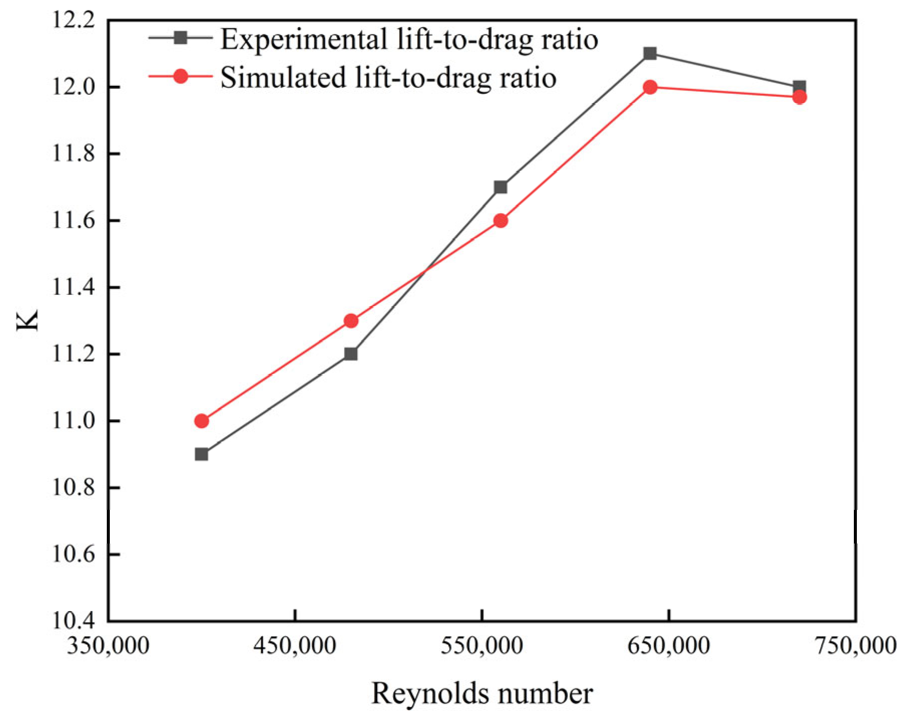
I G D = 1 | R | r R min a A r b 2 1 / 2
where R represents the reference Pareto front; A represents the approximation front; | R | denotes the size of set R (i.e., the number of solutions in the reference Pareto front); r R represents a single solution in the reference Pareto front R ; b A represents a single solution in the approximation front A; r b denotes the Euclidean distance between point r and point b .
The propeller thrust coefficient C T , a dimensionless number that represents the relationship among the propeller thrust, air density, rotational speed, and propeller diameter, was calculated based on the CFD results as follows:
C T = T ρ n 2 D 4 = 3600 T ρ R P M 2 D 4
where T denotes the thrust produced by the propeller (in N), ρ denotes the air density (in kg/m3), n denotes the rotational speed of the propeller (in rev/s), D denotes the propeller diameter (in m), and R P M represents the rotational speed of the propeller (in rev/min).
The lift-to-drag ratio was expressed in this study, and is defined as follows [33]:
K = C l C d
where C l is the lift coefficient and C d is the drag coefficient, both determined from the results of the CFD.
Researchers have implemented the elite-preserving multi-objective evolutionary algorithm NSGA-II (Non-Dominated Sorting Genetic Algorithm II) for optimization tasks [34]. Key algorithmic configurations include 100 individuals per population, 100 evolutionary cycles, a genomic variation probability of 1%, and a gene recombination frequency set at 98% [35]. The NSGA-II framework executes successive generational evolution through probabilistic genetic operators until convergence criteria are met. For this investigation, the optimization target was specifically configured as identifying the vector bracket geometric configuration that simultaneously maximizes both CT and K.

2.7. Validation

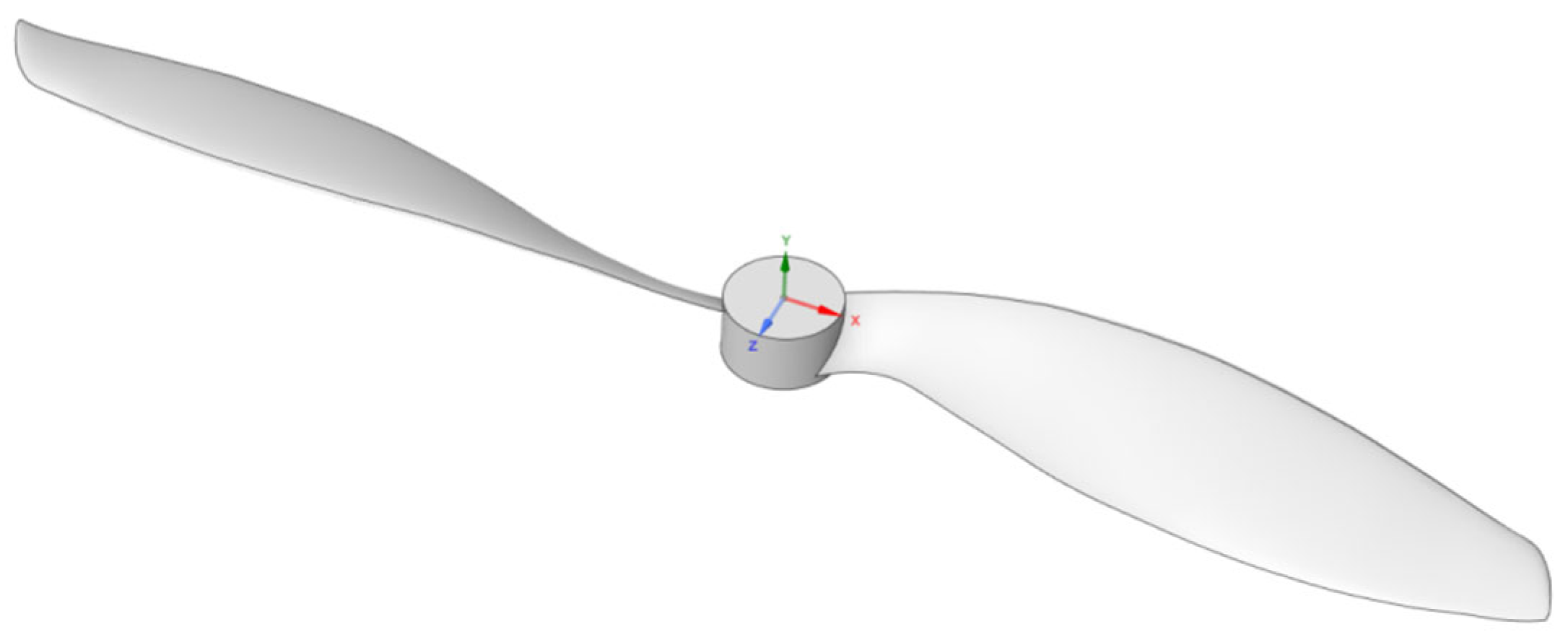
2.7.1. Validation of Propeller Data

(1)
Computational model
The “APC Slow Flyer” standard propeller model shown in Figure 9 was selected to validate the reliability of the solver used in this study. This model has been subjected to a series of wind tunnel tests at the University of Illinois at Urbana–Champaign [36], providing rich experimental data for validation. This propeller model comprises a common two-blade design used in UAVs, and its parameters are listed in Table 3. The propeller material is fiberglass-reinforced plastic.
(2)
Mesh independence verification
The results of numerical simulations often deviate from the results of experiments owing to discretization, approximation, iteration, and rounding errors. In particular, the scale of discretization errors generally decreases as the mesh resolution increases, whereas rounding errors gradually increase. Therefore, both excessively sparse and fine grids can lead to inaccurate results, with the latter also wasting computational resources. The accuracy and computational efficiency of the numerical simulation results were ensured by performing grid-independence verification on the propeller model and selecting an appropriate meshing strategy. The five different mesh configurations shown in Table 4 were generated by adjusting the grid size at the leading and trailing edges of the propeller and the number of boundary layers. A propeller mesh comprising 2.08 million cells was ultimately selected to balance computational efficiency and accuracy.
(3)
Method validation
The C T values of the propeller were calculated at different rotational speeds using Equation (17) and plotted on the line chart in Figure 10 to compare them with those obtained from wind tunnel experiments. The maximum, minimum, and average errors between the simulated and experimental values were 2.5%, 0.2%, and 1.56%, respectively, indicating that the CFD numerical simulation method was reliable and confirming the accuracy of the MRF approach for propeller calculations. Thus, this computational method was used for the numerical simulation of the propeller in this study.

2.7.2. UAV Validation

(1)
Mesh independence verification
For the UAV model, five grid partitioning schemes with varying scales were generated by adjusting the wing leading edge, trailing edge, and boundary layer meshes. Specific data are detailed in Table 5. After a comparative analysis considering both computational efficiency and accuracy, the scheme with 1.86 million grid cells was ultimately selected as the computational mesh for subsequent numerical simulations.
(2)
Method validation
To verify the reliability of the CFD numerical simulation method, the lift-to-drag ratio curves of the UAV at different Reynolds numbers were plotted and comparatively analyzed with the wind tunnel test data. As shown in Figure 11, the numerical simulation results demonstrated good agreement with the experimental data, with a maximum error of 0.9%, minimum error of 0.1%, and average error of 0.7% between simulated and experimental values. This comparison confirmed that the current computational method achieved high accuracy and could be reliably applied to numerical simulation studies of external flow fields for vertical takeoff and landing UAVs.

3. Results and Discussion

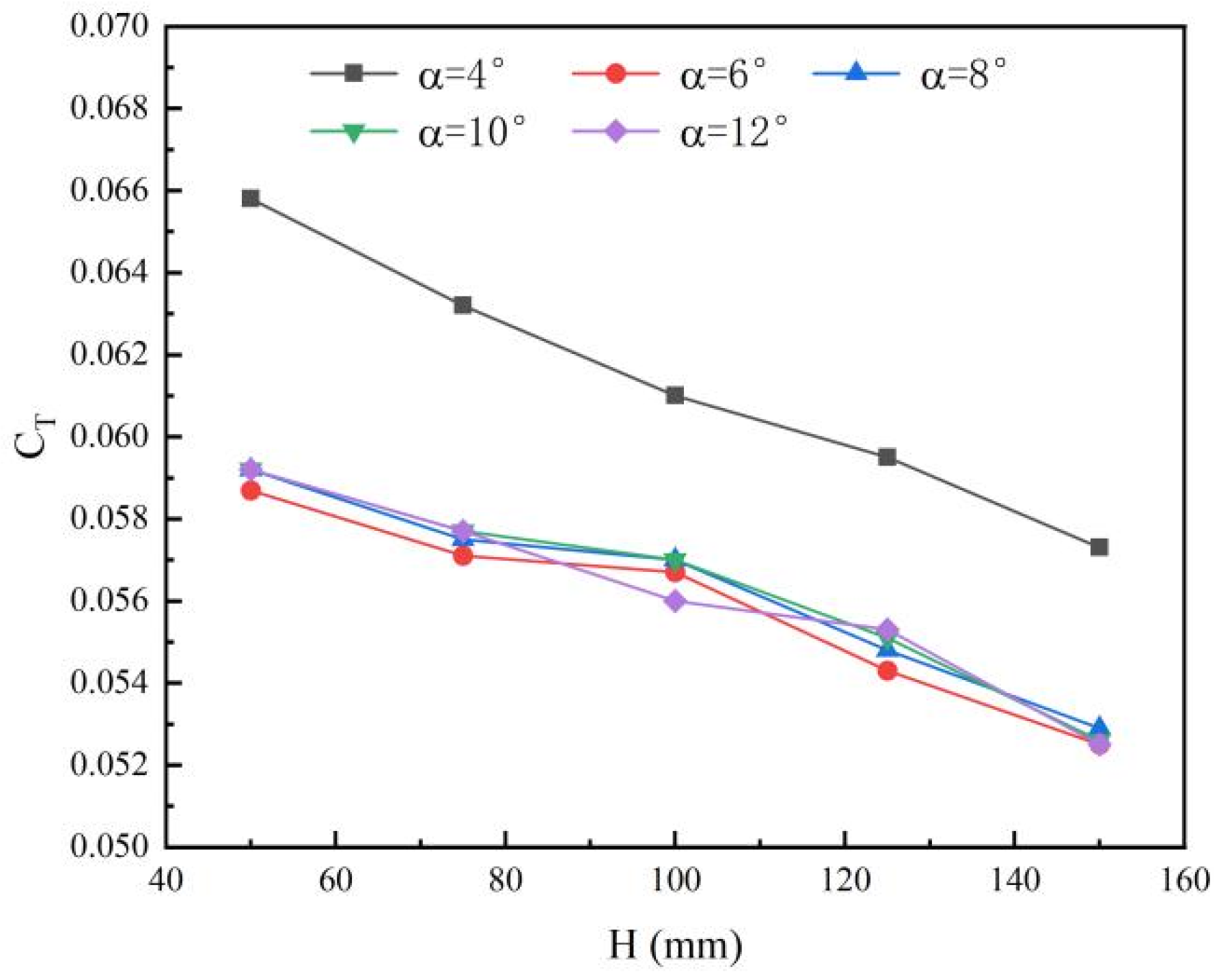
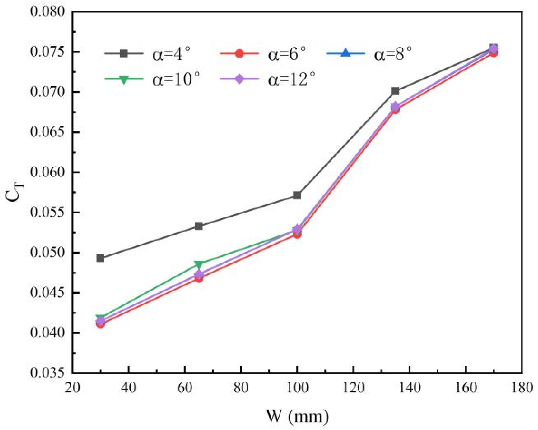
3.1. Impacts of Structural Parameters

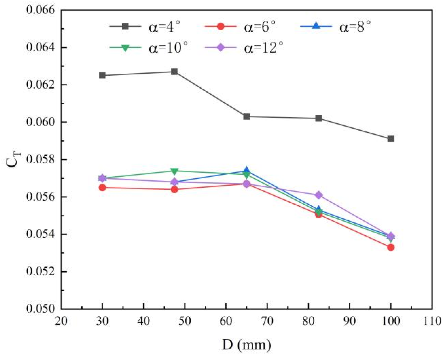
3.1.1. Propeller Thrust Coefficient C T

The effect of H on C T is shown in Figure 12. Given the same angle of attack, C T decreased as H increased because a higher bracket resulted in a smaller area of flow obstruction by the fixed bracket, allowing more incoming flow to directly impact the propeller. When the angle of attack was smaller, the UAV fuselage obstructed a larger area of the incoming flow, resulting in a higher C T .
The effect of L on C T is shown in Figure 13. Given the same angle of attack, C T increased sharply with increasing L. In particular, C T increased by 140% when L increased from 30 mm to 170 mm at a 4° angle of attack. Indeed, C T was confirmed to reach its maximum value when the angle of attack was 4°.
The effect of W on C T is shown in Figure 14. Given the same angle of attack, C T increased linearly as W increased from 30 to 100 mm and from 135 to 170 mm and increased sharply when W increased from 135 to 170 mm.
The effect of D on C T is shown in Figure 15. Given the same angle of attack, C T decreased as D increased. Furthermore, the value of C T reached its maximum when the angle of attack was 4°, indicating optimal propeller performance.

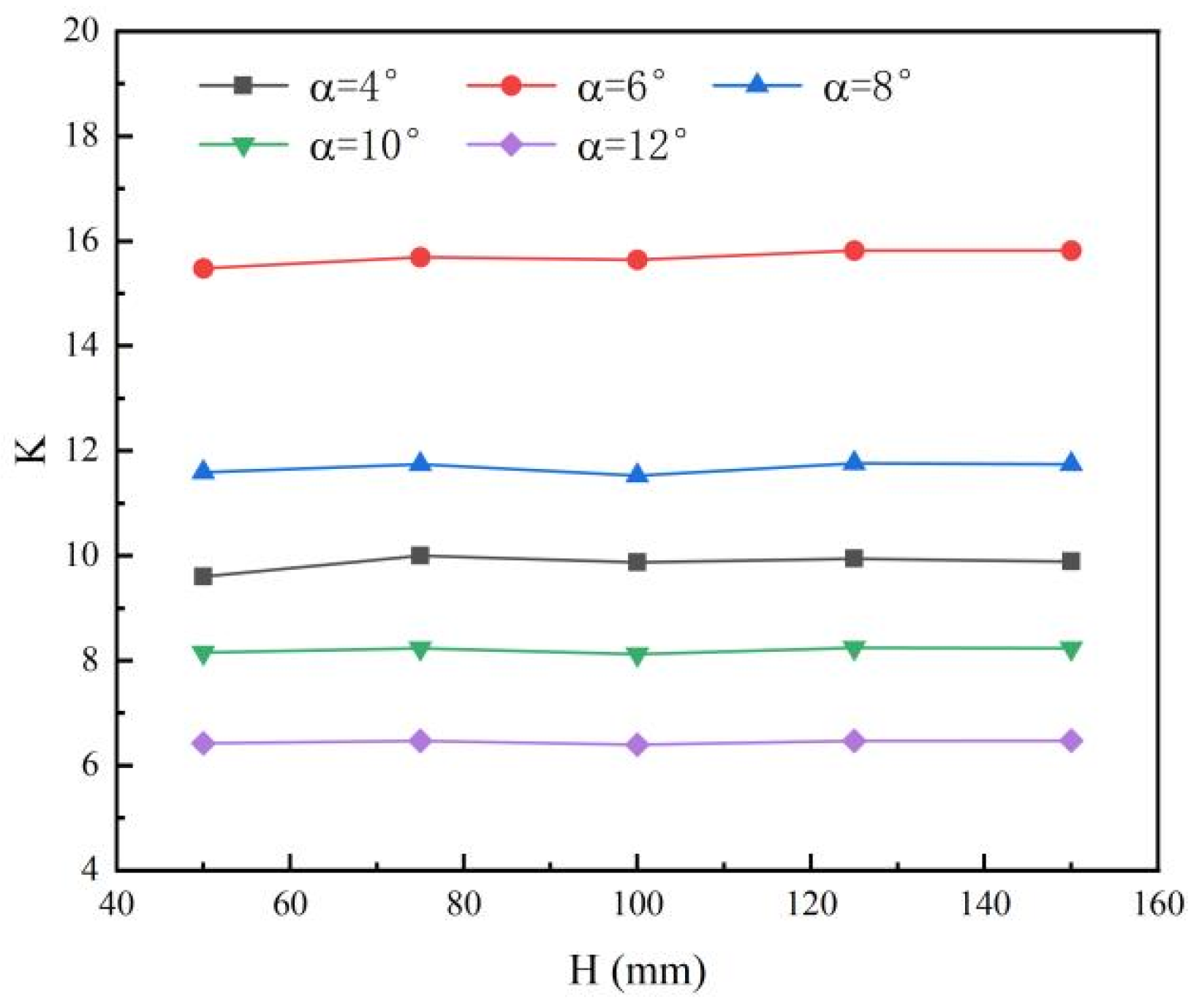
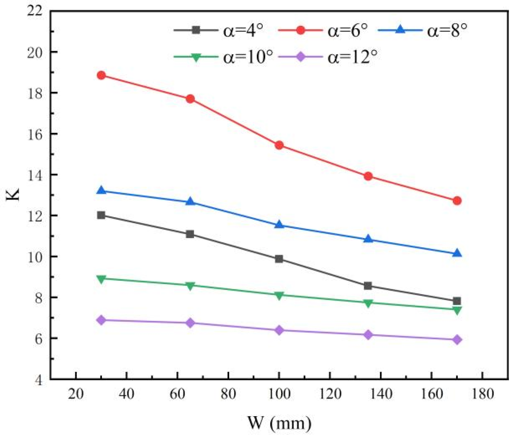
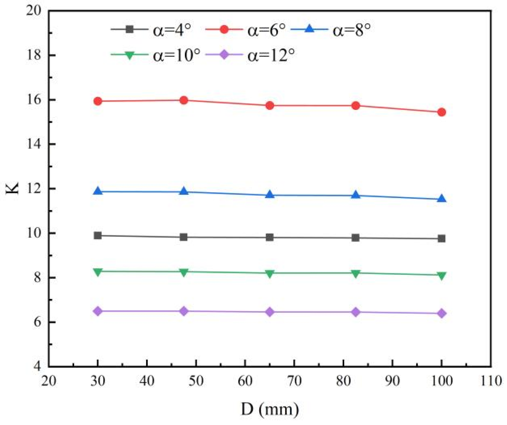
3.1.2. Lift-to-Drag Ratio K

The effect of H on the K of the UAV is illustrated in Figure 16. Given the same angle of attack, K decreased linearly as H increased. Furthermore, the value of K initially increased, then decreased as the angle of attack increased from 4° to 12°. The maximum K was achieved when the angle of attack was 6°.
The effect of L on the K of the UAV is shown in Figure 17. Given the same angle of attack, K decreased as L increased. When the angle of attack was between 4° and 6°, the K value decreased sharply as L increased. When the angle of attack was between 8° and 12°, the K value decreased linearly as L increased.
The effect of W on the K of the UAV is shown in Figure 18. Given the same angle of attack, the K decreased as W increased. When the angle of attack was between 4° and 6°, K decreased sharply with increasing W. When the angle of attack was between 8° and 12°, K decreased linearly as W increased.
Finally, the effect of D on the K of the UAV is shown in Figure 19. Given the same angle of attack, K exhibited no significant change as D increased; therefore, the effect of D on K can be ignored.

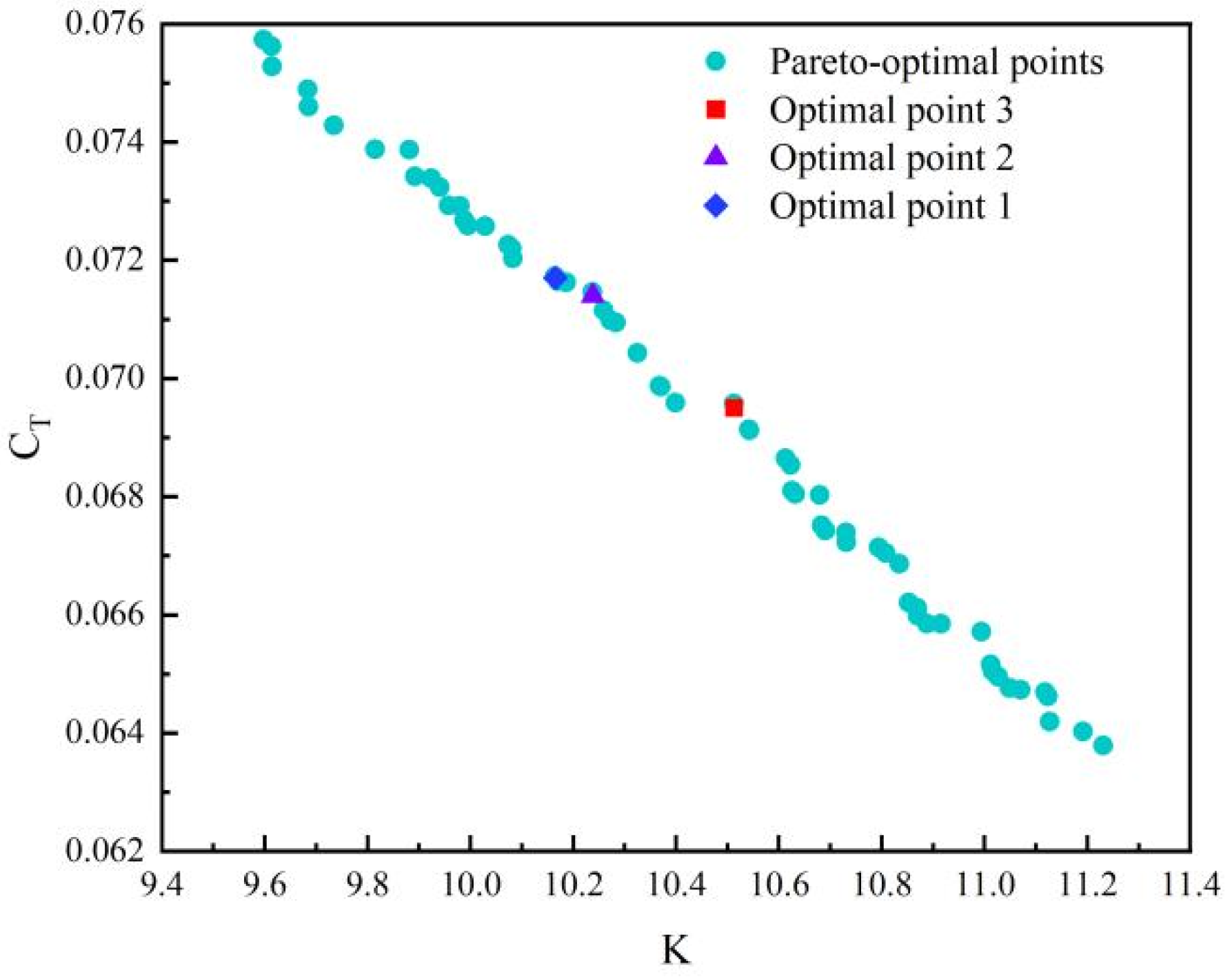
3.2. Multi-Objective Optimization

The maximization of CT and K was used as the objective function to search for the optimal structural parameters across the global range using the MOGA defined in Section 2.5; the initial population was constructed using the screening method; and the RSMs for C T and K were constructed using the kriging algorithm. The results of the MOGA optimization are shown in Figure 20, and three sets of optimal structural parameters were obtained, as listed in Table 6. The average CT and K values of the three optimal models were 18.1% and 4.3% higher than those of the original model. In particular, Optimum 2 exhibited a 19% increase in C T and a 3.7% increase in K , effectively balancing the improvements of these characteristics. Therefore, the final optimal structural parameters for the vector bracket comprised H = 51 mm, L = 168 mm, W = 69 mm, and D = 31 mm. Note that the actual C T and K values obtained by a CFD simulation conducted using the Optimum 2 parameters were 0.0711 and 9.882, respectively. Thus, the value of C T was confirmed to increase by 19%, whereas there was no significant change in K .
A GD value of approximately 0.0124 indicates that the current genetic algorithm solution set was generally close to the reference front, while an IGD value of approximately 0.0087 suggests that the distribution of the reference front was well covered by the solution set. Given that both the GD and IGD are relatively small (<0.1), the current optimization results are deemed to be good.

4. Conclusions

A CCD experiment was employed to construct 25 sample points for four structural parameters describing the vector support bracket of a VTOL UAV in the horizontal flight condition. Numerical CFD simulations were conducted to calculate the propeller thrust and vehicle lift-to-drag ratio for these 25 sample points, the kriging algorithm was applied to construct RSMs for these coefficients, and an MOGA subsequently conducted global optimization to identify the optimal parameters maximizing the two coefficients. The optimal structural parameters for the vector bracket were determined to comprise a vector bracket height of 51 mm, fixed bracket length of 168 mm, fixed bracket width of 69 mm, and ball socket outer diameter of 31 mm. These parameter values resulted in a 19% effective improvement in the propeller thrust coefficient over that of the original UAV model, demonstrating the utility of the proposed optimization method.
Future research on the vector bracket’s lightweight design could focus on two key directions: (1) material optimization through advanced composites like carbon-fiber-reinforced polymers or additive-manufactured lattice structures to achieve optimal strength-to-weight ratios, and (2) topological optimization of the bracket’s architecture using computational design methods to eliminate redundant material while maintaining structural integrity under aerodynamic loads. Particularly, the integration of generative AI-driven design with multi-scale modeling could enable novel lightweight configurations that simultaneously address vibration damping and load-bearing requirements during complex flight maneuvers. Such improvements would directly contribute to enhanced power efficiency and extended flight endurance for next-generation UAV systems.
Note that the precision of the RSM should be enhanced in future studies by developing a multi-objective collaborative response surface using an information-sharing bridge between multiple objective functions. This approach could better capture the complex interdependencies and nonlinear relationships between the two objectives, thereby providing more comprehensive and accurate modeling and guidance for the MOGA optimization. Furthermore, although this study optimized the structural parameters of the vector bracket to improve its performance based on aerodynamic theory, future research should consider the use of novel lightweight, high-strength materials in the vector bracket to reduce weight and enhance structural strength.

Author Contributions

This study was conducted by W.L., who was responsible for the overall research design, simulation modeling, and data analysis, as well as manuscript writing and revision; W.Q. participated in the simulation calculations and result validation; J.W. was in charge of algorithm development and parameter optimization; X.Y. undertook literature review and data visualization tasks; Q.L. (Qingzheng Liu) performed simulation model verification and sensitivity analysis; Q.L. (Qiang Liu) provided computational resources support and project coordination; Y.T. contributed to research discussions and manuscript revisions. All authors collaborated closely to accomplish this simulation-based structural parameter optimization research. All authors have read and agreed to the published version of the manuscript.

Funding

This research was supported by the Shaanxi Provincial Key R&D Program (grant no. 2023-YBGY-385), the Key Research Program Project of Shaanxi Provincial Department of Science and Technology (grant no. 2024NC-YBXM-203), the Shaanxi Provincial Department of Science and Technology General Project (grant no. 2022JM-131), the Special Program for Local Service and Industrialization Cultivation Project of Shaanxi Provincial Department of Education (grant no. 24JC024), and university-level projects at Shaanxi University of Technology (grant no. SLGRCQD2101).

Data Availability Statement

The original contributions presented in this study are included in the article. Further inquiries can be directed to the corresponding author.

Conflicts of Interest

The contact author has declared that none of the authors has any competing interests.

References

  1. Kumar, S.P.; Subeesh, A.; Jyoti, B.; Mehta, C.R. Applications of Drones in Smart Agriculture. In Smart Agriculture for Developing Nations: Status, Perspectives and Challenges; Springer Nature: Singapore, 2023. [Google Scholar] [CrossRef]
  2. Cheng, M.; Sun, C.; Nie, C.; Liu, S.; Yu, X.; Bai, Y.; Liu, Y.; Meng, L.; Jia, X.; Liu, Y.; et al. Evaluation of UAV—Based Drought Indices for Crop Water Conditions Monitoring: A Case Study of Summer Maize. Agric. Water Manag. 2023, 287, 108442. [Google Scholar] [CrossRef]
  3. Eladl, S.G.; ZainEldin, H.Y.; Haikal, A.Y.; Saafan, M.M. Smart Agriculture Based On IOT Using Drones: A Survey. Mansoura Eng. J. 2024, 49, 10. [Google Scholar] [CrossRef]
  4. Nduku, L.; Munghemezulu, C.; Mashaba-Munghemezulu, Z.; Kalumba, A.M.; Chirima, G.J.; Masiza, W.; De Villiers, C. Global Research Trends for Unmanned Aerial Vehicle Remote Sensing Application in Wheat Crop Monitoring. Geomatics 2023, 3, 115–136. [Google Scholar] [CrossRef]
  5. Ndlovu, H.S.; Odindi, J.; Sibanda, M.; Mutanga, O. A Systematic Review on the Application of UAV—Based Thermal Remote Sensing for Assessing and Monitoring Crop Water Status in Crop Farming Systems. Int. J. Remote Sens. 2024, 45, 4923–4960. [Google Scholar] [CrossRef]
  6. Li, B.; Sun, J.; Zhou, W.; Wen, C.-Y.; Low, K.H.; Chen, C.-K. Transition Optimization for a VTOL Tail-Sitter UAV. IEEE/ASME Trans. Mechatron. 2020, 25, 2534–2545. [Google Scholar] [CrossRef]
  7. Li, H.; Liu, K. Aerodynamic Design Optimization and Analysis of Ducted Fan Blades in DEP UAVs. Aerospace 2023, 10, 153. [Google Scholar] [CrossRef]
  8. Czyba, R.; Lemanowicz, M.; Gorol, Z.; Kudala, T. Construction Prototyping, Flight Dynamics Modeling, and Aerodynamic Analysis of Hybrid VTOL Unmanned Aircraft. J. Adv. Transp. 2018, 2018, 7040531. [Google Scholar] [CrossRef]
  9. Lee, S.; Oh, S.; Choi, S.; Lee, Y.; Park, D. Numerical Analysis on Aerodynamic Performances and Characteristics of Quad Tilt Rotor During Forward Flight. J. Korean Soc. Aeronaut. Space Sci. 2018, 46, 197–209. [Google Scholar] [CrossRef]
  10. Karali, H.; Inalhan, G.; Tsourdos, A. Advanced UAV Design Optimization Through Deep Lea-rning-Based Surrogate Models. Aerospace 2024, 11, 669. [Google Scholar] [CrossRef]
  11. Laghari, A.A.; Jumani, A.K.; Laghari, R.A.; Nawaz, H. Unmanned Aerial Vehicles: A Review. Cogn. Robot. 2023, 3, 8–22. [Google Scholar] [CrossRef]
  12. Shirazi, M.; Khademalrasoul, A.; Ardebili, S.M.S. Multi-Objective Optimization of Soil Erosion Parameters Using Response Surface Method (RSM) in the Emamzadeh Watershed. Acta Geophys. 2020, 68, 505–517. [Google Scholar] [CrossRef]
  13. Verma, A.; Sharma, S.; Pramanik, H. Rapid Identification of Optimized Process Parameters via RSM for the Production of Valuable Aromatic Hydrocarbons Using Multiphase Catalytic Pyrolysis of Mixed Waste Plastics. Arab. J. Sci. Eng. 2023, 48, 16527–16542. [Google Scholar] [CrossRef]
  14. Powar, R.V.; Aware, V.V.; Shahare, P.U. Optimizing Operational Parameters of Finger Millet Threshing Drum Using RSM. J. Food Sci. Technol. 2019, 56, 3481–3491. [Google Scholar] [CrossRef]
  15. Eskandari, B.; Bhowmick, S.; Alpas, A.T. Turning of Inconel 718 Using Liquid Nitrogen: Multi-Objective Optimization of Cutting Parameters Using RSM. Int. J. Adv. Manuf. Technol. 2022, 120, 3077–3101. [Google Scholar] [CrossRef]
  16. Li, B.; Tian, X.; Zhang, M. Modeling and Multi-Objective Optimization of Cutting Parameters in High-Speed Milling Using RSM and Improved TLBO Algorithm. Int. J. Adv. Manuf. Technol. 2020, 111, 2323–2335. [Google Scholar] [CrossRef]
  17. Negemiya, A.A.; Rajakumar, S.; Balasubramanian, V. Optimization of Ti-6Al-4V/AISI304 Diffusion Bonding Process Parameters Using RSM and PSO Algorithm. Multidiscip. Model. Mater. Struct. 2019, 15, 1037–1052. [Google Scholar] [CrossRef]
  18. Zhu, W.; Yu, X.; Wang, Y. Layout Optimization for Blended Wing Body Aircraft Structure. Int. J. Aeronaut. Space Sci. 2019, 20, 879–890. [Google Scholar] [CrossRef]
  19. Panwar, V.; Sharma, D.K.; Kumar, K.V.P.; Jain, A.; Thakar, C. Experimental Investigations and Optimization of Surface Roughness in Turning of EN 36 Alloy Steel Using Response Surface Methodology and Genetic Algorithm. Mater. Today Proc. 2021, 46, 6474–6481. [Google Scholar] [CrossRef]
  20. Park, G.; Oh, K.Y.; Nam, W. Parent Nested Optimizing Structure for Vibration Reduction in Floating Wind Turbine Structures. J. Mar. Sci. Eng. 2020, 8, 876. [Google Scholar] [CrossRef]
  21. Ebrahimi, M.J.; Pasandidehfard, M.; Esmaeili, A.; Esfandabadi, M.H.M. Optimization of Aerodynamic Design of a Winged UAV Through Genetic Algorithms and Large Eddy Simulation. Int. J. Aerosp. Eng. 2024, 2024, 2698950. [Google Scholar] [CrossRef]
  22. Zhang, Z.; Xie, C.; Huang, K.; Yang, C. Influence of Aerodynamic Interaction on Performance of Contrarotating Propeller/Wing System. Aerospace 2022, 9, 813. [Google Scholar] [CrossRef]
  23. Sun, C.; Zhao, W. Analysis of Aerodynamic Interaction Between Mounted Propeller and Twin-Tailboom UAV. J. Ordnance Equip. Eng. 2021, 42, 118–122. [Google Scholar]
  24. Shi, W.; Li, J. Impacts of Propeller Installation Effect on Aerodynamic Performances for UAV. J. Aero-Space Power 2020, 35, 611–619. [Google Scholar]
  25. Shi, W.; Li, J.; Zhao, S.; Yang, Z. Investigation and Improvement of Pusher-Propeller Installation Effect for Flying Wing UAV. Int. J. Aeronaut. Space Sci. 2021, 22, 287–302. [Google Scholar] [CrossRef]
  26. Guo, Q.; Zhu, Y.; Tang, Y.; Hou, C.; He, Y.; Zhuang, J.; Zheng, Y.; Luo, S. CFD simulation and experimental verification of the spatial and temporal distributions of the downwash airflow of a quad-rotor agricultural UAV in hover. Comput. Electron. Agric. 2020, 172, 105343. [Google Scholar] [CrossRef]
  27. Yashwanth, C.; Anushkka, V.; Datthathireyan, K.D.; Srinithi, M.; Aamir, H.; Kumar, G.D.; Arulmozhi, K. Computational Fluid Dynamics Analysis of a Coaxial Unmanned Aerial Vehicle; SAE Technical Paper; SAE International: Warrendale, PA, USA, 2024. [Google Scholar] [CrossRef]
  28. Zhang, Z. Structure Design of Tailstock Vertical Take-Off and Landing UAV. Master’s Thesis, Henan University of Technology, Zhengzhou, China, 2020. [Google Scholar]
  29. Chang, M.; Zheng, Z.; Meng, X.; Bai, J.; Wang, B. Aerodynamic Analysis of a Low-Speed Tandem-Channel Wing for eVTOL Air-craft Considering Propeller–Wing Interaction. Energies 2022, 15, 8616. [Google Scholar] [CrossRef]
  30. Sikirica, A.; Čarija, Z.; Kranjčević, L.; Lučin, I. Grid Type and Turbulence Model Influence on Propeller Characteristics Prediction. J. Mar. Sci. Eng. 2019, 7, 374. [Google Scholar] [CrossRef]
  31. Ameen, F.; Mathivanan, K.; Zhang, R.; Ravi, G.; Rajasekar, S. One Factor at a Time and Two-Factor Optimization of Transesterification Parameters Through Central Composite Design (CCD) for the Conversion of Used Peanut Oil (UPNO) to Biodiesel. Fuel 2023, 352, 129065. [Google Scholar] [CrossRef]
  32. Toal, D.J.J. Applications of multi-fidelity multi-output Kriging to engineering design optimization. Struct. Multidiscip. Optim. 2023, 66, 125. [Google Scholar] [CrossRef]
  33. Yao, X.; Liu, W.; Han, W.; Li, G.; Ma, Q. Development of Response Surface Model of Endurance Time and Structural Parameter Optimization for a Tail-Sitter UAV. Sensors 2020, 20, 1766. [Google Scholar] [CrossRef]
  34. Verma, S.; Pant, M.; Snasel, V. A Comprehensive Review on NSGA-II for Multi-Objective Combinatorial Optimization Problems. IEEE Access 2021, 9, 57757–57791. [Google Scholar] [CrossRef]
  35. Ma, H.; Zhang, Y.; Sun, S.; Liu, T.; Shan, Y. A Comprehensive Survey on NSGA-II for Multi-Objective Optimization and Applications. Artif. Intell. Rev. 2023, 56, 15217–15270. [Google Scholar] [CrossRef]
  36. Brandt, J.B. Small-Scale Propeller Performance at Low Speeds. Master’s Thesis, University of Illinois at Urbana-Champaign, Champaign-Urbana, IL, USA, 2005. [Google Scholar]
Figure 1. Structure of the considered UAV, including key components such as the propeller, winglets, and servo systems: 1—winglet, 2—wing, 3—propeller, 4—motor, 5—ball socket, 6—ball joint bearing, 7—fixed bracket, 8—universal joint, 9—push rod, 10—servo.
Aerospace 12 00487 g001
Figure 2. Geometric parameters of the considered VTOL UAV: (a) winglets (side view) and (b) wing (top view).
Aerospace 12 00487 g002
Figure 3. Structural parameters of the vector bracket.
Aerospace 12 00487 g003
Figure 4. Division of rotating and stationary domains.
Aerospace 12 00487 g004
Figure 5. Schematic diagram of the mesh for the stationary and rotating domains.
Aerospace 12 00487 g005
Figure 6. Flow chart of structural parameter optimization.
Aerospace 12 00487 g006
Figure 7. Circumscribed CCD sample points.
Aerospace 12 00487 g007
Figure 8. Optimization process of genetic algorithm.
Aerospace 12 00487 g008
Figure 9. APC Slow Flyer propeller model [35].
Aerospace 12 00487 g009
Figure 10. Simulation verification for the propeller.
Aerospace 12 00487 g010
Figure 11. Simulation result validation of the unmanned aerial vehicle.
Aerospace 12 00487 g011
Figure 12. Effect of H on C T at different angles of attack.
Aerospace 12 00487 g012
Figure 13. Effect of L on C T at different angles of attack.
Aerospace 12 00487 g013
Figure 14. Effect of W on C T at different angles of attack.
Aerospace 12 00487 g014
Figure 15. Effect of D on C T at different angles of attack.
Aerospace 12 00487 g015
Figure 16. Effect of H on C F A at different angles of attack.
Aerospace 12 00487 g016
Figure 17. Effect of L on C F A at different angles of attack.
Aerospace 12 00487 g017
Figure 18. Effect of W on K at different angles of attack.
Aerospace 12 00487 g018
Figure 19. Effect of D on K at different angles of attack.
Aerospace 12 00487 g019
Figure 20. MOGA optimization.
Aerospace 12 00487 g020
Table 1. Geometric parameters of the considered VTOL UAV wing.
ParameterValue
Wingspan b (mm)1200
Wing root chord c r (mm)500
Wing tip chord c t (mm)300
Wing sweep angle Λ w (°)28
Spanwise length at the winglet tip l y s (mm)280
Winglet sweep angle Λ v (°)56
Winglet height l v (mm)30
Winglet thickness h (mm)6
Winglet support foot length l j c (mm)200
UAV flight angle of attack a (°)4–12
Table 2. Range of the structural parameters of the selected vector bracket.
Structural ParameterLower LimitUpper Limit
Fixed bracket length L (mm)30170
Fixed bracket width W (mm)30170
Vector bracket height H (mm)50150
Ball socket outer diameter D (mm)30100
Table 3. Geometric parameters of the propeller used for validation.
Propeller ParameterValue
ModelAPC Slow Flyer
Rotational diameter (mm)254
Pitch (mm)177.8
Hub diameter (mm)18
Hub height (mm)10
Table 4. Mesh independence verification of the propeller model.
Mesh Count (Millions)Thrust Coefficient C T
1.760.146
1.850.1465
1.930.1471
2.080.1477
2.120.148
Table 5. Mesh independence verification for the UAV model.
Mesh Count (Millions)Lift-to-Drag Ratio k
11111.8
12111.86
14211.89
18611.94
22412
Table 6. Optimal structural parameters.
ParameterOriginal
Model
Optimal
Point 1
Validate 1
Optimal
Optimal
Point 2
Validate 2
Optimal
Optimal Point 3Validate 3
Optimal
H10050.9251.1956.32
L100169.65168.38169.5
W10065.4768.970.32
D6531.6330.9530.07
CT0.060.06950.06910.07140.07110.07170.0701
Optimization gain (%)-15.80.5190.419.52.2
K 9.8710.51310.21110.2389.88210.1659.938
Optimization gain (%)-6.52.93.73.62.92.28
Disclaimer/Publisher’s Note: The statements, opinions and data contained in all publications are solely those of the individual author(s) and contributor(s) and not of MDPI and/or the editor(s). MDPI and/or the editor(s) disclaim responsibility for any injury to people or property resulting from any ideas, methods, instructions or products referred to in the content.

