

RBF-Learning-Based Many-Objective Metaheuristic for Robust and Optimal Controller Design in Fixed-Structure Heading Autopilot


Abstract
1. Introduction
2. Formulation of the Robust Optimal Fixed-Structure Heading Autopilot Design Problem
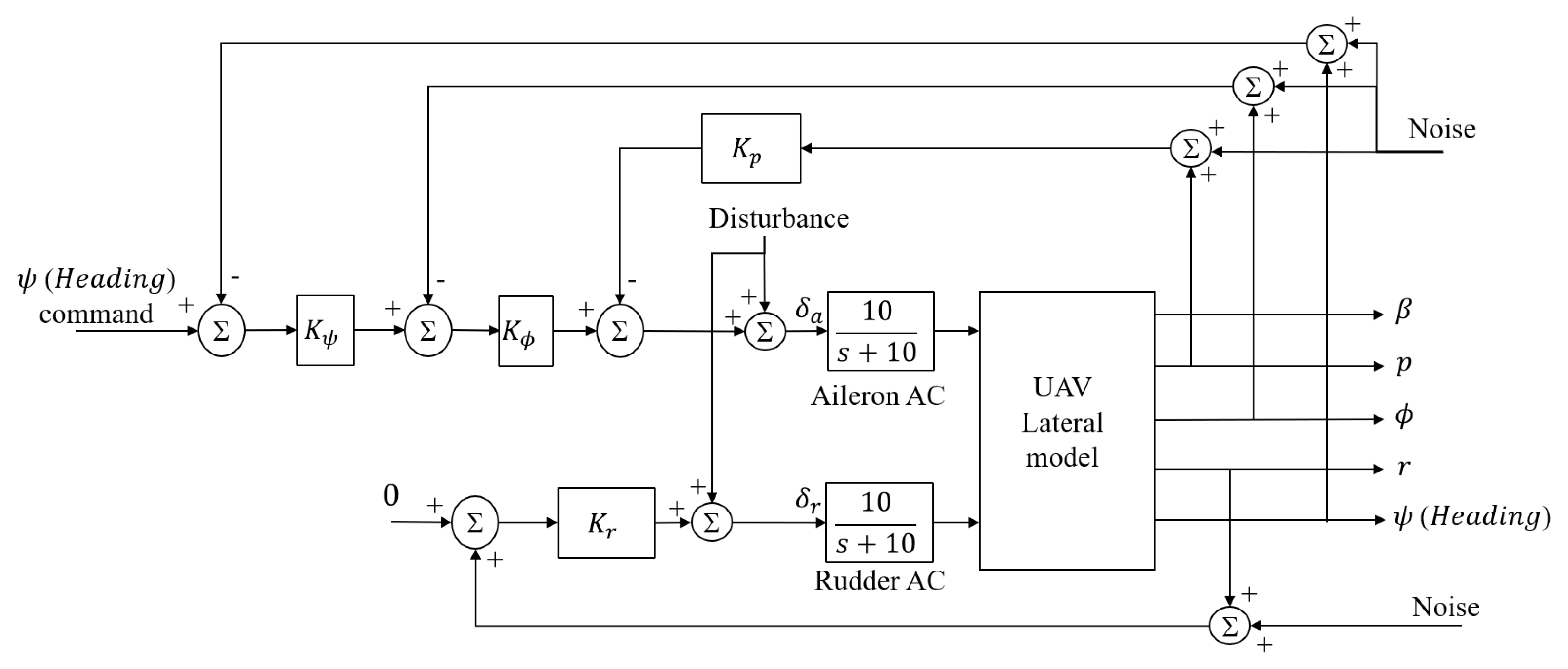
2.1. UAV Model Utilized in This Study
2.2. Robust Optimum Fixed-Structure Heading Autopilot Design Approach
- is the input signal,
- is the output signal,
- are flight controllers,
- is the control signal,
- G = plant model, which includes an actuator, and,
- Δ = additive perturbation or uncertainty in the plant model.
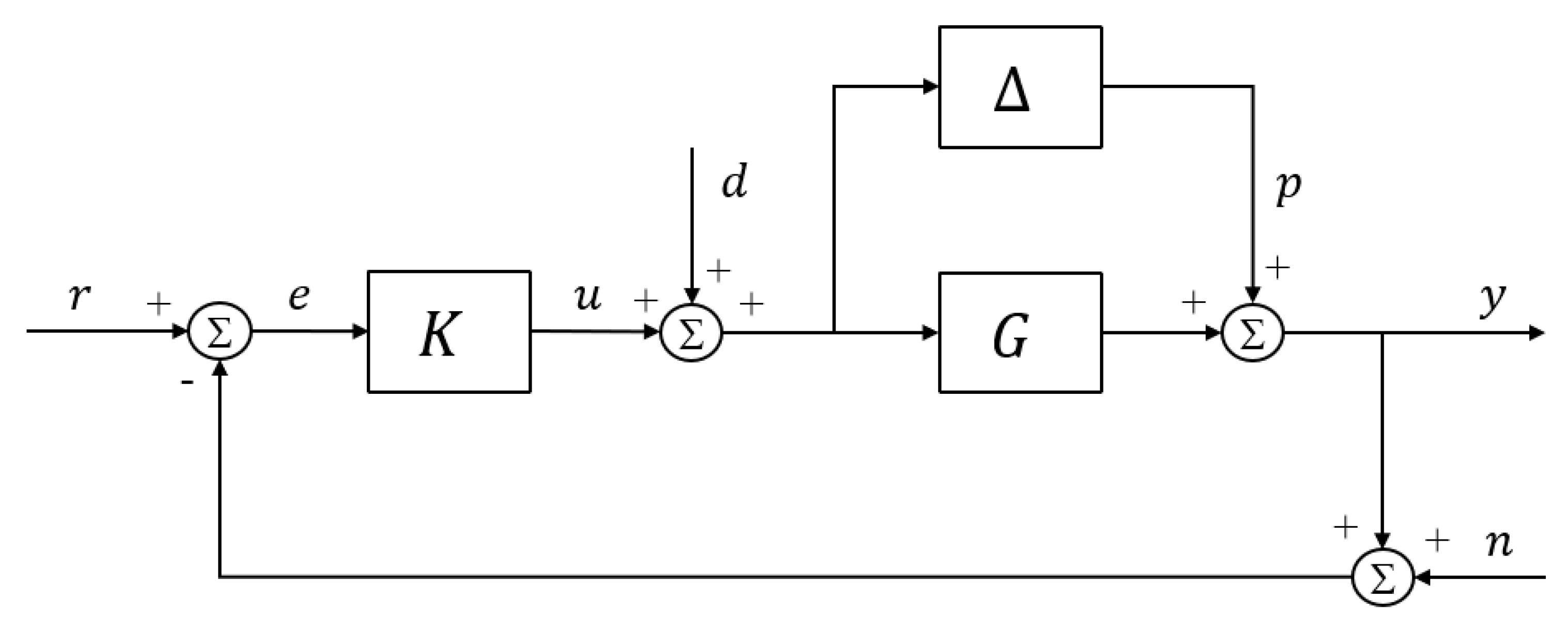
- For good reference tracking (r→e)
- For good handling perturbation or uncertainty (p→u)
- For good gust disturbance attenuation (d→y)
- For good noise rejection (n→y)
- For less control energy (r→u)
2.3. Optimization Problem for a Robust Many-Objective Fixed-Structure Heading Autopilot Controller Design
| , | |
| , | , |
| , | , |
| , | , |
| , | , |
| To achieve accurate heading reference tracking. | |
| To effectively handle perturbations or uncertainties while minimizing control energy. | |
| For effective attenuation of gust disturbances. | |
| For effective noise rejection. |
3. RBF-Learning-Based A-MRPBIL-DE for Many-Objective Optimization
3.1. Self-Adaptive Multi-Objective Real-Code Population-Based Incremental Learning Hybridized with Differential Evolution (A-MRPBIL-DE)
| Algorithm 1. A-MRPBIL-DE. |
| Input: Number of iterations (NG), population size (NP), number of design domain subintervals (nI), number of trays (NT), and Pareto archive size (NA). Output: A Main Procedure Initialization 1: Define Pij = nI/Np for each tray, a Pareto archive A = {}. 2: Generate a real-code population X from the probability trays and evaluate objective function values. 3: Select non-dominated solutions from X∪A and save them to A. 4: Set initial PMum = 0.5, Pxrm = 0.5, Fm = 0.5, CRm = 0.5. 5: Set initial goodPMum = {}, goodPxrm = {}, goodCR = {} and goodF = {}. 6: For i = 1 to NG. Update the population using the RPBIL operation 7: Divide the non-dominated solutions into NT groups using a clustering technique and find the centroid rG of each group. 8: Update the probability trays using rG. 9: Generate a real code population X from the probability trays. Update the population using a DE operation 10: For j = 1 to NP 10.1: Generate PMu, Pxr, and CR by a random normal distribution and generate F by the Lehmer mean technique. 10.2: Randomly select a solution xbest from Pareto archive A. 10.3: Randomly select four solutions, xr1, xr2, xr3, and xr4. 10.3.1 If rand < Pxr, select the xr1, xr2, xr3, and xr4 from the current population X. 10.3.2 Otherwise, select the xr1, xr2, xr3, and xr4 from Pareto archive A. 10.4: Generate a new solution using the mutation schemes in Equation (6). 10.5: Perform crossover schemes in Equation (7). 10.6: Save the newly generated solution in Y. 11: End. 12: Evaluate objective function values of the new population. Pareto selection 13: Select non-dominated solutions from Y∪A and save as A. For each yi∈Y that dominates at least one solution in A, the parameters, PMu, Pxr, CR, and F index i are saved to goodPMu, goodPxr, goodCR, and goodF, respectively. Processing parameter adaption 14: Update the parameters, PMum, Pxrm Fm, and CRm using Equations (8)–(11). 15: If the number of A is larger than NA, remove some of the members in A using a clustering technique. 16: End. |
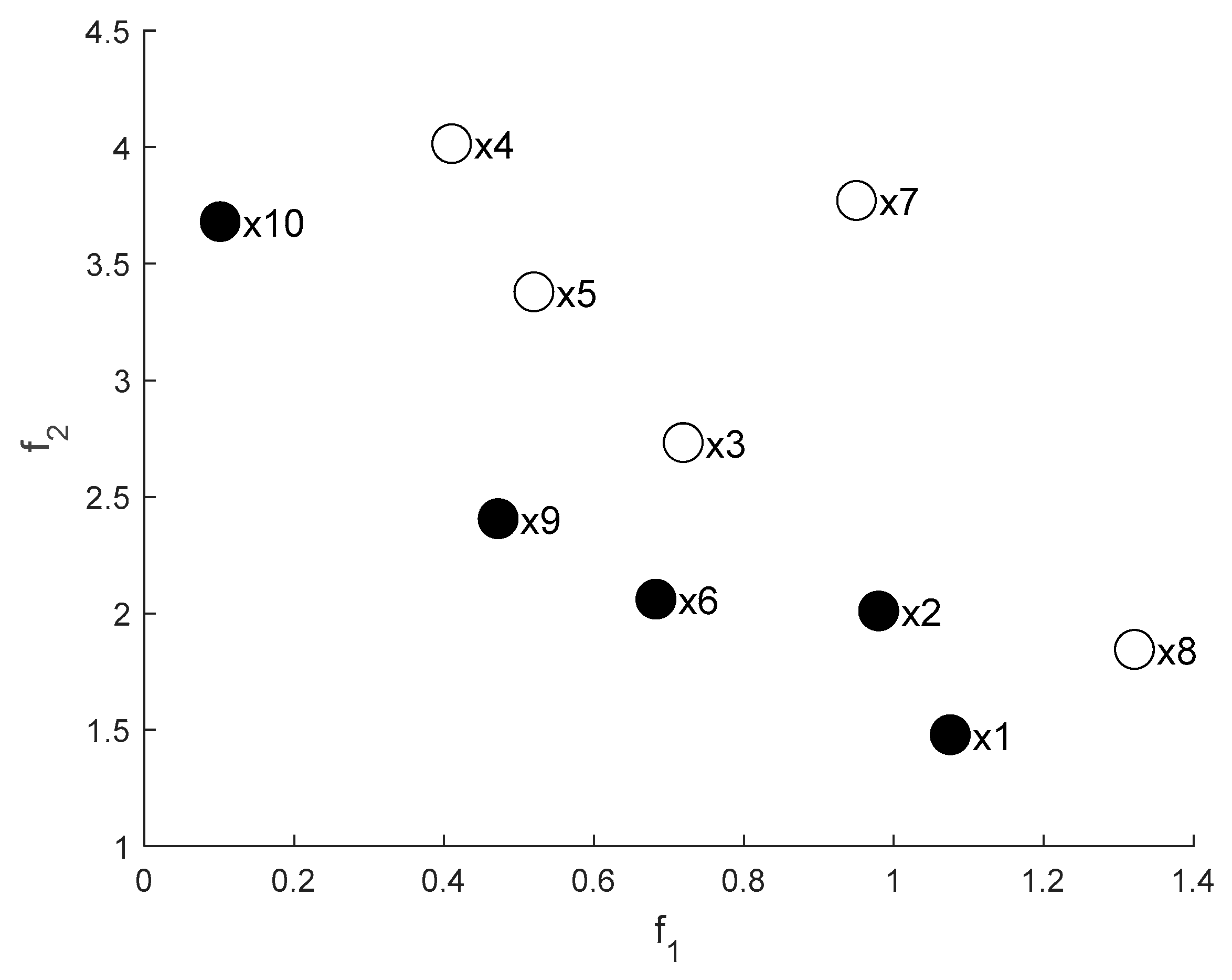
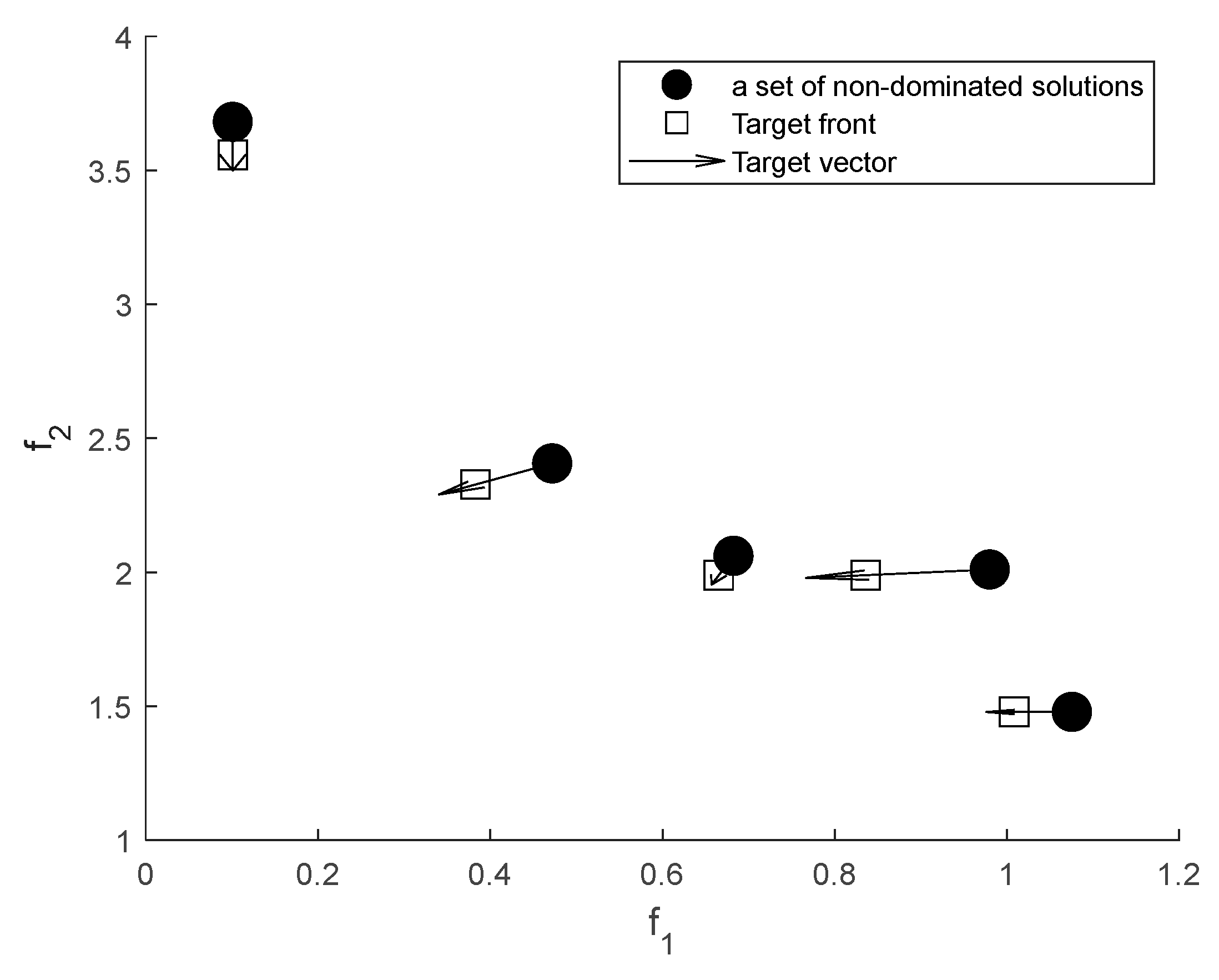
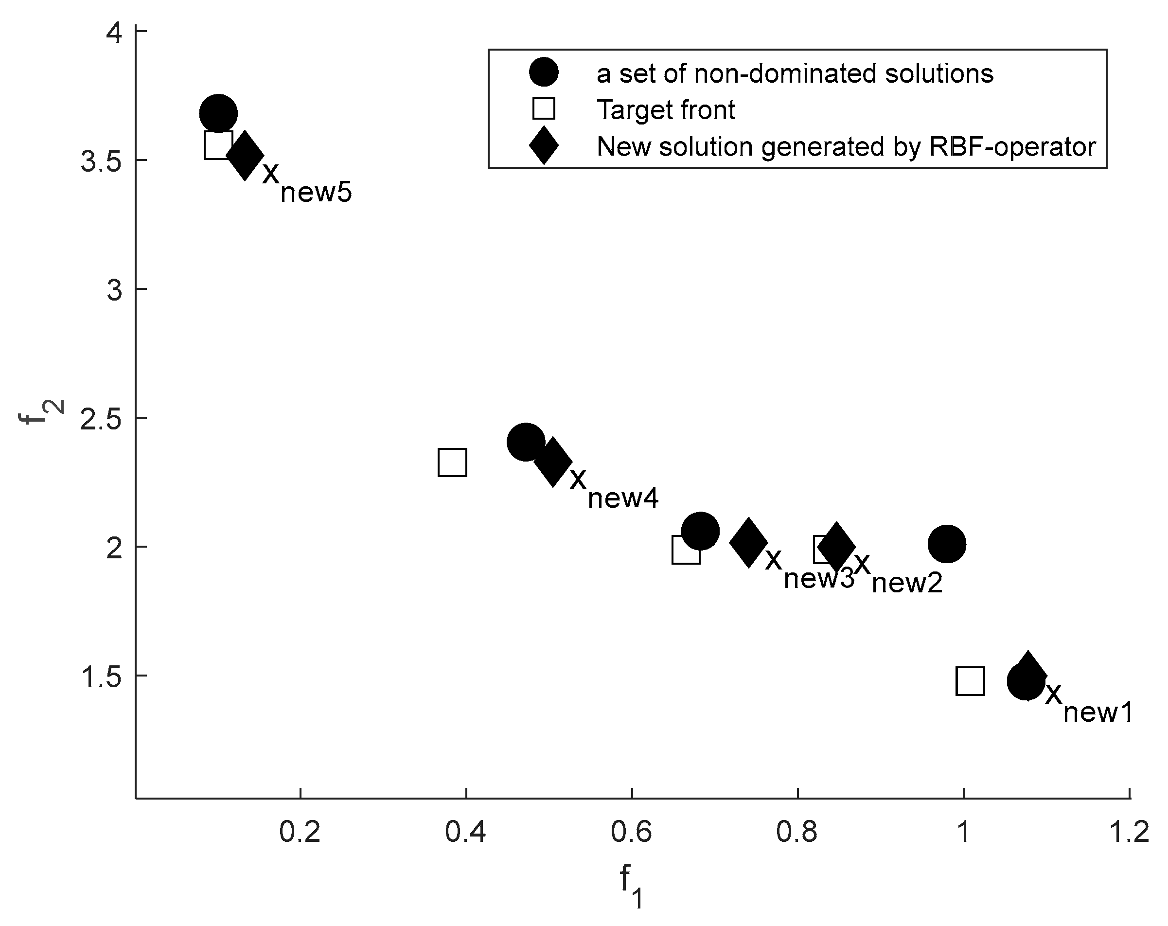
3.2. RBF-Learning-Based A-MRPBIL-DE
| Algorithm 2 A-MRPBIL-DE-RBF |
| Input: Number of iterations (NG), population size (NP), number of design domain subintervals (nI), number of trays (NT), Pareto archive size (NA), population size of the RBF operation (NRBF). Output: A Main Procedure Initialization 1: Define Pij = nI/Np for each tray, a Pareto archive A = {}. 2: Generate a real-coded population X from the probability trays and evaluate objective function values. 3: Select non-dominated solutions from X∪A and save them to A. 4: Set initial PMum = 0.5, Pxrm = 0.5, Fm = 0.5, CRm = 0.5. 5: Set initial goodPMum = {}, goodPxrm = {}, goodCR = {} and goodF = {}. 6: nFEs = 0 and maxFEs = NG × NP. 7: While nFEs < maxFE. Update population using RPBIL operation 8: Divide the non-dominated solutions into NT groups using a clustering technique and find the centroid rG of each group. 9: Update the probability trays using rG. 10: Generate a real-code population X from the probability trays. Update population using a DE operation 11: For j = 1 to NP. 11.1: Generate PMu, Pxr, and CR by normal random distribution and generate F using the Lehmer mean technique. 11.2: Randomly select a solution xbest from the Pareto archive A. 11.3: Randomly select four solutions, xr1, xr2, xr3, and xr4. 11.3.1 If rand < Pxr, select the xr1, xr2, xr3, and xr4 from the current population X. 11.3.2 Otherwise, select the xr1, xr2,xr3, and xr4 from Pareto archive A. 11.4: Generate a new solution using the mutation schemes in Equation (6). 11.5: Perform crossover schemes in Equation (7). 11.6: Save the newly generated solution in Y. 12: End. 13: Evaluate objective function values of the new population in Y. 14: nFEs = nFEs + NP. RBF-learning operation 15: Randomly select NRBF points in a set of non-dominated solutions. 16: For j = 1 to NRBF. 16.1: Compute the target point using Equation (17). 16.2: Apply Equation (14) to generate a new solution. 16.3: Save the newly generated solution in Z. 17: End. 18: Evaluate objective function values of the new population in Z. 19: nFEs = nFEs + NRBF. Pareto selection 20: Select non-dominated solutions from Z∪Y∪A and save them as A. For each yi∈Y that dominates at least one solution in A, the parameters, PMu, Pxr, CR, and F index i are saved to goodPMu, goodPxr, goodCR, and goodF, respectively. Processing parameter adaption 21: Update the parameters, PMum, Pxrm Fm, and CRm using Equations (8)–(11). 22: If the number of A is larger than NA, remove some of the members in A using a clustering technique. 23: End. |
4. Numerical Experiments
- A knee point-driven evolutionary algorithm for many-objective optimization (MnKnEA) [35];
- A reference vector-guided evolutionary algorithm for many-objective optimization (RVEA) [36];
- Multi-objective Grey Wolf Optimizer: a novel algorithm for multi-criterion optimization (MOGWO) [37];
- An evolutionary many-objective optimization algorithm using reference-point-based non-dominated sorting (NSGA-III) [38];
- Success history-based adaptive multi-objective differential evolution (SHAMODE) [39];
- Hybrid real-code population-based incremental learning and differential evolution algorithm (MRPBIL-DE) [29];
- Hybrid real code population-based incremental learning and differential evolutionary algorithm with adaptive parameters (A-MRPBIL-DE) [27];
- A-MRPBIL-DE-RBF (Algorithm 2).
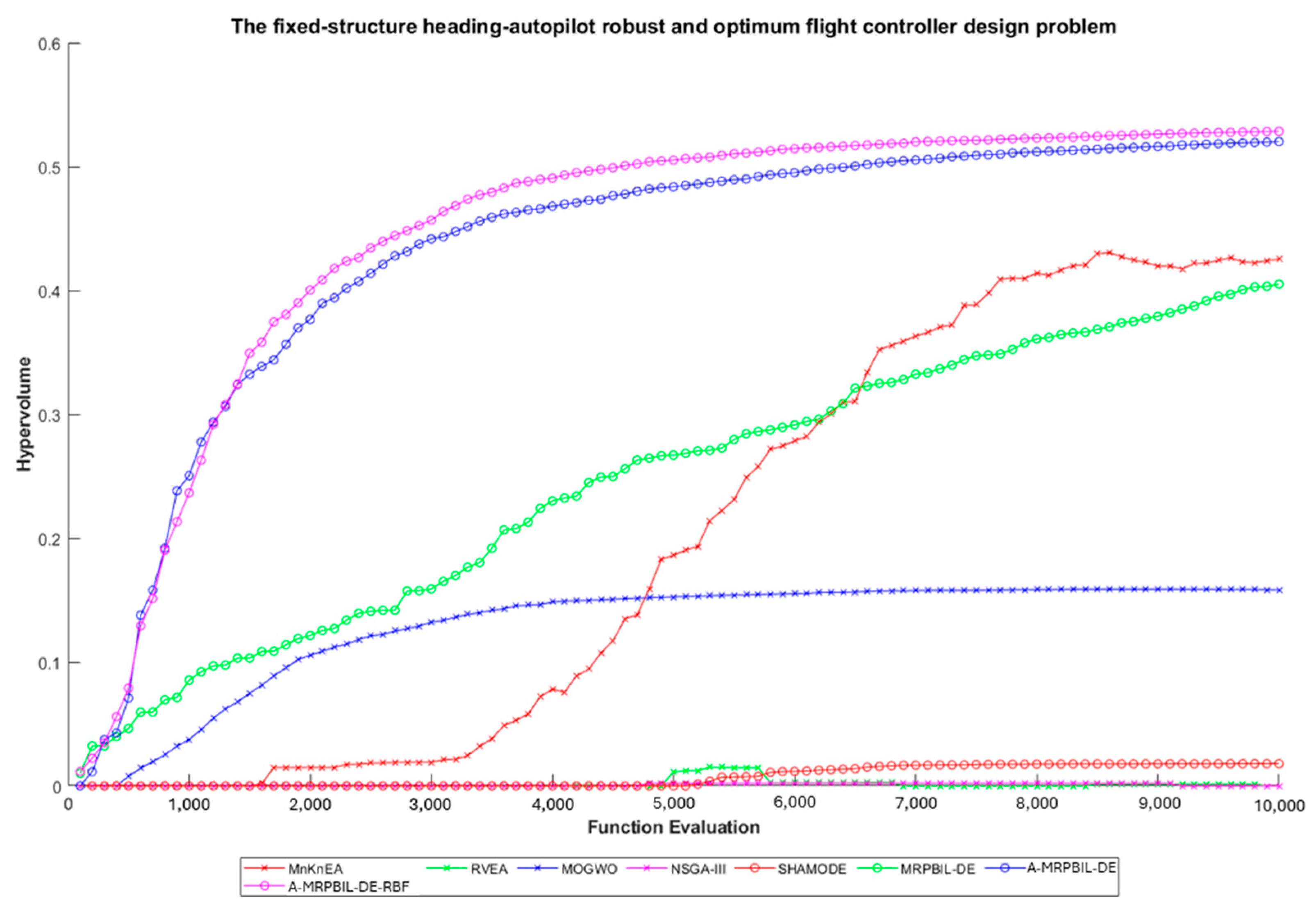
5. Results and Discussion
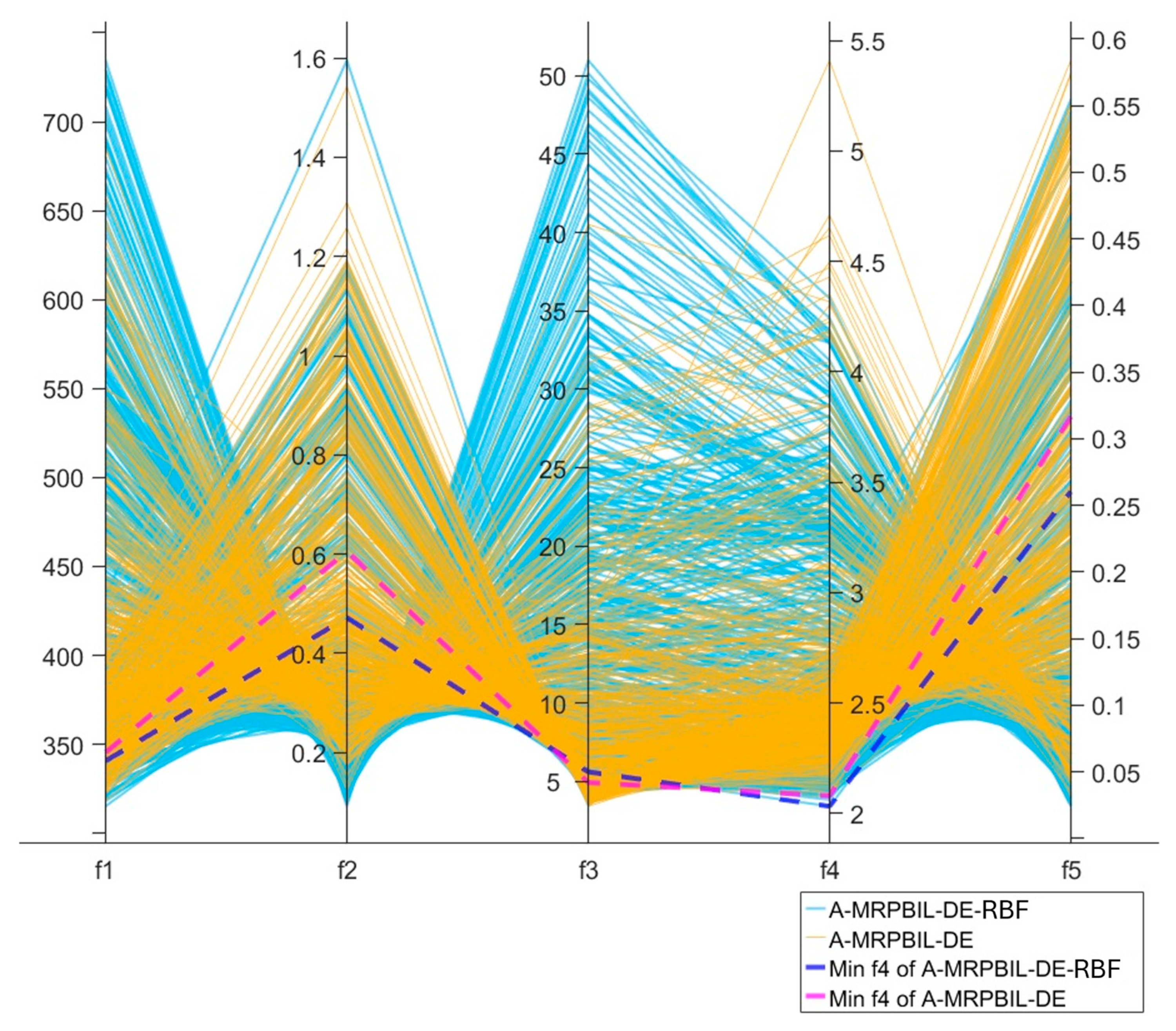
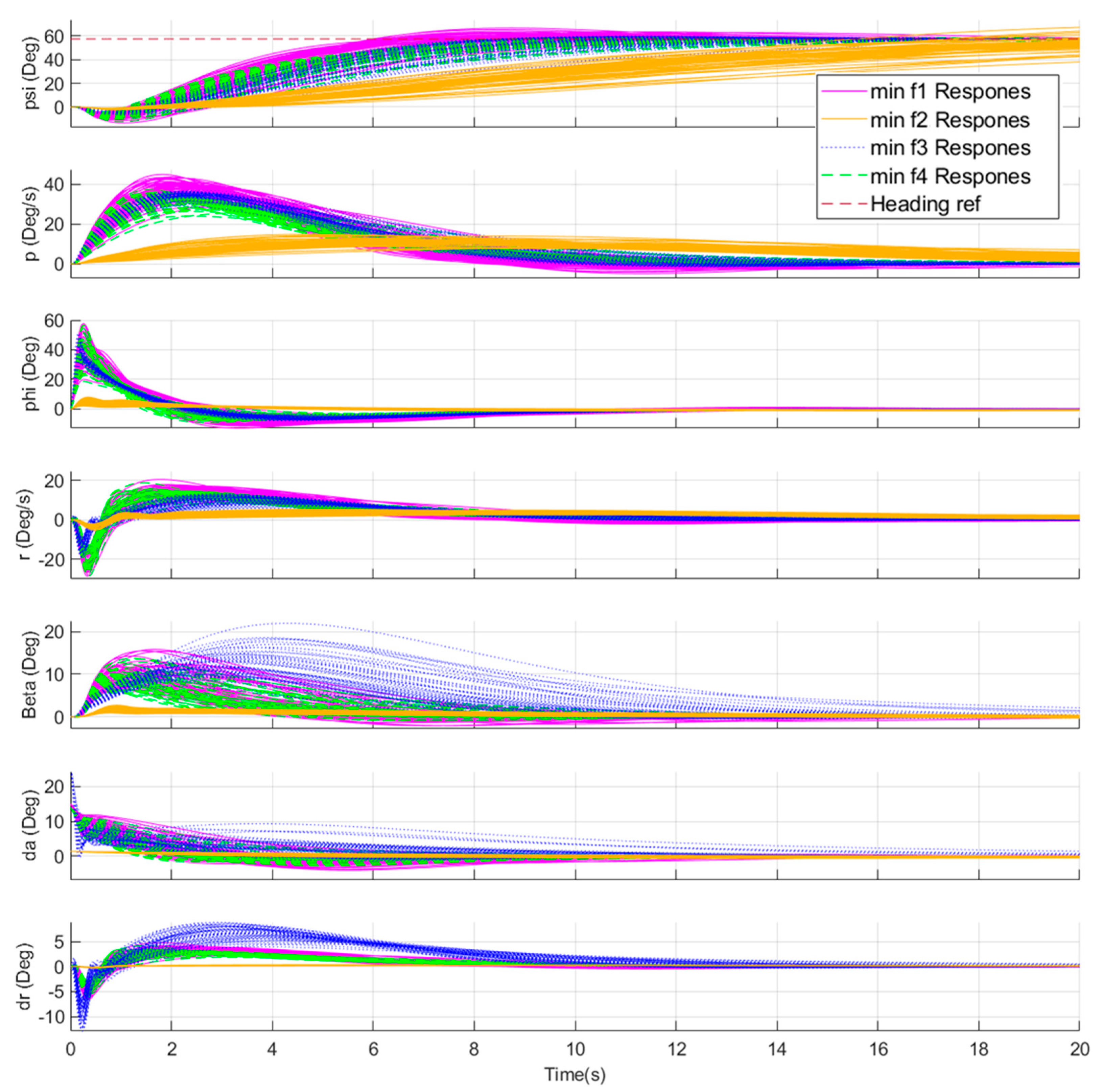
5.1. Robust Optimum Fixed-Structure Heading Autopilot Flight Controller Design Problem
5.2. The Benchmark Test Suites
5.3. The Real-World Test Problems
6. Conclusions
Author Contributions
Funding
Data Availability Statement
Conflicts of Interest
Appendix A. Benchmark Test Suites and the Performance Indicators, Including HV, STE, GD, and IGD

| Problems | MnKnEA | RVEA | MOGWO | NSGA_III | SHAMODE | MRPBIL-DE | A-MRPBIL-DE | A-MRPBIL-DE-RBF |
|---|---|---|---|---|---|---|---|---|
| MaF1 | 2.154 × 10⁻¹ [2.83] | 1.853 × 10⁻¹ [6.07] | 2.115 × 10⁻¹ [3.80] | 1.616 × 10⁻¹ [7.73] | 2.166 × 10⁻¹ [2.60] | 1.680 × 10⁻¹ [7.20] | 2.066 × 10⁻¹ [4.77] | 2.264 × 10⁻¹ [1.00] |
| MaF2 | 2.119 × 10⁻¹ [2.00] | 2.056 × 10⁻¹ [3.97] | 2.060 × 10⁻¹ [3.97] | 1.717 × 10⁻¹ [8.00] | 2.052 × 10⁻¹ [4.63] | 1.984 × 10⁻¹ [7.00] | 2.043 × 10⁻¹ [5.43] | 2.141 × 10⁻¹ [1.00] |
| MaF5 | 4.740 × 10⁻¹ [4.47] | 5.055 × 10⁻¹ [5.03] | 3.833 × 10⁻¹ [6.47] | 2.595 × 10⁻¹ [7.73] | 5.369 × 10⁻¹ [3.40] | 4.866 × 10⁻¹ [5.60] | 5.521 × 10⁻¹ [2.20] | 5.650 × 10⁻¹ [1.10] |
| MaF6 | 1.831 × 10⁻¹ [4.00] | 1.926 × 10⁻² [7.18] | 1.196 × 10⁻¹ [5.63] | 9.818 × 10⁻³ [7.72] | 2.001 × 10⁻¹ [1.00] | 1.290 × 10⁻¹ [5.47] | 1.974 × 10⁻¹ [2.63] | 1.976 × 10⁻¹ [2.37] |
| MaF7 | 2.666 × 10⁻¹ [2.00] | 2.021 × 10⁻¹ [6.33] | 2.075 × 10⁻¹ [5.83] | NA [8.00] | 2.461 × 10⁻¹ [4.00] | 2.532 × 10⁻¹ [3.57] | 2.361 × 10⁻¹ [4.97] | 2.716 × 10⁻¹ [1.30] |
| MaF8 | 7.562 × 10⁻⁴ [4.70] | 2.278 × 10⁻⁴ [6.52] | 1.812 × 10⁻⁴ [6.57] | 3.526 × 10⁻⁴ [5.93] | 7.527 × 10⁻³ [1.67] | 1.401 × 10⁻⁴ [6.28] | 7.082 × 10⁻³ [2.43] | 7.124 × 10⁻³ [1.90] |
| MaF9 | NA [5.17] | 1.341 × 10⁻⁴ [4.92] | NA [5.17] | 1.032 × 10⁻⁴ [4.05] | NA [5.17] | 1.834 × 10⁻⁴ [3.78] | 2.851 × 10⁻⁴ [3.40] | 2.347 × 10⁻⁴ [4.35] |
| MaF10 | 7.461 × 10⁻¹ [1.00] | 4.199 × 10⁻¹ [2.00] | 7.328 × 10⁻² [6.93] | 2.262 × 10⁻² [7.97] | 2.889 × 10⁻¹ [3.00] | 1.077 × 10⁻¹ [5.93] | 1.463 × 10⁻¹ [4.50] | 1.412 × 10⁻¹ [4.67] |
| MaF11 | 9.155 × 10⁻¹ [1.00] | 8.966 × 10⁻¹ [2.80] | 8.929 × 10⁻¹ [3.37] | 7.814 × 10⁻¹ [7.70] | 8.903 × 10⁻¹ [3.87] | 7.976 × 10⁻¹ [7.23] | 8.452 × 10⁻¹ [6.03] | 8.883 × 10⁻¹ [4.00] |
| MaF12 | 5.164 × 10⁻¹ [2.67] | 4.981 × 10⁻¹ [4.93] | 5.240 × 10⁻¹ [2.00] | 3.365 × 10⁻¹ [8.00] | 5.160 × 10⁻¹ [3.37] | 4.350 × 10⁻¹ [6.57] | 4.408 × 10⁻¹ [6.17] | 5.167 × 10⁻¹ [2.30] |
| MaF13 | 4.488 × 10⁻¹ [5.20] | 4.403 × 10⁻¹ [5.80] | 3.606 × 10⁻¹ [7.60] | 3.956 × 10⁻¹ [7.00] | 5.038 × 10⁻¹ [2.07] | 4.708 × 10⁻¹ [4.17] | 5.029 × 10⁻¹ [2.23] | 5.047 × 10⁻¹ [1.93] |
| MaF14 | NA [5.52] | NA [5.52] | 3.030 × 10⁻³ [5.38] | NA [5.52] | NA [5.52] | 1.029 × 10⁻² [5.03] | 9.091 × 10⁻² [1.52] | 7.860 × 10⁻² [2.00] |
| MaF15 | 2.015 × 10⁻⁴ [6.07] | NA [6.15] | 1.557 × 10⁻¹ [2.10] | NA [6.15] | 1.609 × 10⁻¹ [1.57] | 1.203 × 10⁻¹ [2.33] | 1.082 × 10⁻⁴ [6.07] | 8.912 × 10⁻³ [5.57] |
| DTLZ2 | 6.696 × 10⁻¹ [3.00] | 6.829 × 10⁻¹ [1.60] | 5.785 × 10⁻¹ [4.90] | 3.681 × 10⁻¹ [8.00] | 4.902 × 10⁻¹ [6.40] | 4.853 × 10⁻¹ [6.50] | 5.957 × 10⁻¹ [4.20] | 6.844 × 10⁻¹ [1.40] |
| DTLZ4 | 6.450 × 10⁻¹ [1.93] | 6.583 × 10⁻¹ [1.97] | 4.580 × 10⁻¹ [6.07] | 2.800 × 10⁻¹ [7.80] | 4.651 × 10⁻¹ [6.17] | 4.902 × 10⁻¹ [5.80] | 6.244 × 10⁻¹ [3.63] | 6.534 × 10⁻¹ [2.63] |
| DTLZ5 | 7.229 × 10⁻² [3.23] | 1.201 × 10⁻¹ [1.03] | 6.557 × 10⁻² [3.63] | 1.094 × 10⁻³ [8.00] | 4.529 × 10⁻² [4.73] | 1.695 × 10⁻² [6.67] | 2.220 × 10⁻² [6.17] | 9.084 × 10⁻² [2.53] |
| DTLZ6 | 2.288 × 10⁻² [3.07] | 1.119 × 10⁻² [3.40] | 1.955 × 10⁻² [1.77] | NA [5.75] | NA [5.75] | NA [5.75] | 3.105 × 10⁻⁴ [5.45] | 8.075 × 10⁻³ [5.07] |
| WFG2 | 9.647 × 10⁻¹ [1.00] | 9.390 × 10⁻¹ [2.00] | 9.097 × 10⁻¹ [3.13] | 7.638 × 10⁻¹ [7.63] | 8.565 × 10⁻¹ [4.97] | 7.894 × 10⁻¹ [6.87] | 8.019 × 10⁻¹ [6.47] | 8.892 × 10⁻¹ [3.93] |
| WFG4 | 7.195 × 10⁻¹ [1.00] | 6.851 × 10⁻¹ [2.00] | 4.119 × 10⁻¹ [7.73] | 4.297 × 10⁻¹ [7.27] | 6.002 × 10⁻¹ [4.30] | 5.676 × 10⁻¹ [5.87] | 5.883 × 10⁻¹ [4.83] | 6.445 × 10⁻¹ [3.00] |
| WFG7 | 7.330 × 10⁻¹ [1.17] | 7.182 × 10⁻¹ [1.83] | 4.105 × 10⁻¹ [7.00] | 2.663 × 10⁻¹ [8.00] | 5.202 × 10⁻¹ [4.03] | 4.787 × 10⁻¹ [5.67] | 4.871 × 10⁻¹ [5.30] | 5.721 × 10⁻¹ [3.00] |
| WFG8 | 5.745 × 10⁻¹ [1.27] | 5.650 × 10⁻¹ [1.73] | 1.921 × 10⁻¹ [7.80] | 2.269 × 10⁻¹ [7.20] | 4.252 × 10⁻¹ [4.17] | 4.076 × 10⁻¹ [5.30] | 4.055 × 10⁻¹ [5.50] | 4.511 × 10⁻¹ [3.03] |
| WFG9 | 6.861 × 10⁻¹ [1.07] | 6.392 × 10⁻¹ [2.17] | 3.817 × 10⁻¹ [7.10] | 2.573 × 10⁻¹ [7.90] | 5.433 × 10⁻¹ [4.20] | 4.692 × 10⁻¹ [5.97] | 5.257 × 10⁻¹ [4.83] | 6.106 × 10⁻¹ [2.77] |
| Sum ranks | 63.35 | 84.95 | 113.95 | 159.05 | 86.57 | 124.55 | 98.73 | 60.85 |
| Ranking | 2 | 3 | 6 | 8 | 4 | 7 | 5 | 1 |
| Problems | MnKnEA | RVEA | MOGWO | NSGA_III | SHAMODE | MRPBIL-DE | A-MRPBIL-DE | A-MRPBIL-DE-RBF |
|---|---|---|---|---|---|---|---|---|
| MaF1 | 1.761 × 10⁻² [6.90] | 1.920 × 10⁻² [6.90] | 7.496 × 10⁻³ [4.90] | 1.947 × 10⁻² [7.20] | 3.445 × 10⁻³ [1.90] | 6.554 × 10⁻³ [4.07] | 4.174 × 10⁻³ [2.90] | 3.143 × 10⁻³ [1.23] |
| MaF2 | 1.278 × 10⁻² [6.70] | 1.191 × 10⁻² [6.33] | 7.631 × 10⁻³ [5.00] | 1.928 × 10⁻² [7.97] | 3.542 × 10⁻³ [1.53] | 4.751 × 10⁻³ [4.00] | 4.160 × 10⁻³ [2.97] | 3.500 × 10⁻³ [1.50] |
| MaF5 | 2.196 × 10⁻² [6.10] | 2.066 × 10⁻² [6.23] | 1.465 × 10⁻² [4.67] | 6.417 × 10⁻² [7.47] | 7.140 × 10⁻³ [2.80] | 8.588 × 10⁻³ [3.50] | 7.388 × 10⁻³ [2.83] | 7.112 × 10⁻³ [2.40] |
| MaF6 | 7.475 × 10⁻³ [4.00] | 1.125 × 10⁻¹ [7.33] | 2.919 × 10⁻² [5.63] | 8.789 × 10⁻² [7.20] | 1.114 × 10⁻³ [1.00] | 3.402 × 10⁻² [5.83] | 3.229 × 10⁻³ [2.63] | 2.902 × 10⁻³ [2.37] |
| MaF7 | 1.361 × 10⁻² [6.00] | 2.143 × 10⁻² [7.20] | 4.781 × 10⁻³ [2.90] | 3.078 × 10⁻² [7.80] | 5.188 × 10⁻³ [2.63] | 5.178 × 10⁻³ [2.77] | 6.194 × 10⁻³ [4.07] | 5.035 × 10⁻³ [2.63] |
| MaF8 | 3.753 × 10⁻² [5.27] | 3.000E+19 [7.32] | 9.205 × 10⁻³ [1.78] | 2.667E+19 [6.97] | 3.709 × 10⁻³ [2.40] | 1.333E+19 [4.47] | 7.360 × 10⁻³ [4.00] | 7.192 × 10⁻³ [3.80] |
| MaF9 | 1.393 × 10⁻² [4.03] | 2.690 × 10⁷ [7.90] | 7.468 × 10⁻² [6.97] | 3.067 × 10⁻² [5.10] | 9.223 × 10⁻³ [2.90] | 1.045 × 10⁻² [2.73] | 1.039 × 10⁻² [2.93] | 1.157 × 10⁻² [3.43] |
| MaF10 | 3.467 × 10⁻² [3.30] | 6.865 × 10⁻² [7.43] | 5.294 × 10⁻² [6.03] | 5.595 × 10⁻² [6.43] | 2.178 × 10⁻² [1.50] | 3.719 × 10⁻² [3.47] | 3.638 × 10⁻² [3.47] | 4.433 × 10⁻² [4.37] |
| MaF11 | 1.886 × 10⁻² [7.77] | 1.320 × 10⁻² [5.87] | 8.587 × 10⁻³ [3.63] | 1.696 × 10⁻² [7.20] | 9.667 × 10⁻³ [4.10] | 6.868 × 10⁻³ [1.93] | 9.271 × 10⁻³ [3.87] | 6.377 × 10⁻³ [1.63] |
| MaF12 | 1.649 × 10⁻² [6.90] | 1.524 × 10⁻² [6.23] | 7.953 × 10⁻³ [5.00] | 2.402 × 10⁻² [7.87] | 5.081 × 10⁻³ [1.93] | 5.676 × 10⁻³ [3.40] | 5.207 × 10⁻³ [2.27] | 5.147 × 10⁻³ [2.40] |
| MaF13 | 3.092 × 10⁻² [6.57] | 3.455 × 10⁻² [6.93] | 2.473 × 10⁻² [5.73] | 2.578 × 10⁻² [5.60] | 1.430 × 10⁻² [3.23] | 1.194 × 10⁻² [2.77] | 1.364 × 10⁻² [3.00] | 1.029 × 10⁻² [2.17] |
| MaF14 | 1.892 × 10⁻² [3.90] | 8.893 × 10⁻² [7.10] | 4.401 × 10⁻² [5.53] | 1.378 × 10⁻² [2.57] | 3.600 × 10⁻² [5.43] | 8.692 × 10⁻² [6.37] | 2.013 × 10⁻² [2.67] | 1.323 × 10⁻² [2.43] |
| MaF15 | 2.206 × 10⁻² [6.60] | 4.858 × 10⁻² [7.93] | 1.153 × 10⁻² [4.53] | 6.581 × 10⁻³ [2.93] | 2.011 × 10⁻² [6.20] | 9.277 × 10⁻³ [4.33] | 4.477 × 10⁻³ [1.97] | 3.900 × 10⁻³ [1.50] |
| DTLZ2 | 2.919 × 10⁻² [7.53] | 2.415 × 10⁻² [6.13] | 1.463 × 10⁻² [4.63] | 2.880 × 10⁻² [7.33] | 6.886 × 10⁻³ [1.53] | 1.351 × 10⁻² [4.37] | 9.207 × 10⁻³ [2.90] | 7.019 × 10⁻³ [1.57] |
| DTLZ4 | 2.734 × 10⁻² [7.13] | 2.645 × 10⁻² [6.80] | 8.067 × 10⁻³ [1.53] | 3.167 × 10⁻² [6.10] | 1.161 × 10⁻² [3.60] | 1.116 × 10⁻² [3.27] | 1.269 × 10⁻² [4.33] | 1.130 × 10⁻² [3.23] |
| DTLZ5 | 1.413 × 10⁻² [6.03] | 4.997 × 10⁻² [7.90] | 7.242 × 10⁻³ [4.90] | 2.876 × 10⁻² [7.07] | 5.405 × 10⁻³ [3.10] | 5.994 × 10⁻³ [3.60] | 4.914 × 10⁻³ [2.27] | 4.219 × 10⁻³ [1.13] |
| DTLZ6 | 1.483 × 10⁻² [5.90] | 3.590 × 10⁻² [7.80] | 1.267 × 10⁻² [5.33] | 2.856 × 10⁻² [6.77] | 7.111 × 10⁻³ [2.13] | 9.517 × 10⁻³ [4.00] | 7.426 × 10⁻³ [2.10] | 7.147 × 10⁻³ [1.97] |
| WFG2 | 1.948 × 10⁻² [7.10] | 1.534 × 10⁻² [6.13] | 1.104 × 10⁻² [4.87] | 2.292 × 10⁻² [7.70] | 9.122 × 10⁻³ [3.67] | 7.632 × 10⁻³ [2.00] | 8.331 × 10⁻³ [2.87] | 7.391 × 10⁻³ [1.67] |
| WFG4 | 3.086 × 10⁻² [7.30] | 2.341 × 10⁻² [6.00] | 1.704 × 10⁻² [5.00] | 3.254 × 10⁻² [7.70] | 1.074 × 10⁻² [1.20] | 1.143 × 10⁻² [1.90] | 1.245 × 10⁻² [3.73] | 1.219 × 10⁻² [3.17] |
| WFG7 | 2.796 × 10⁻² [7.60] | 2.296 × 10⁻² [6.27] | 1.558 × 10⁻² [5.00] | 2.601 × 10⁻² [7.13] | 1.027 × 10⁻² [1.17] | 1.153 × 10⁻² [3.13] | 1.169 × 10⁻² [3.40] | 1.107 × 10⁻² [2.30] |
| WFG8 | 3.603 × 10⁻² [7.97] | 2.381 × 10⁻² [6.20] | 1.797 × 10⁻² [5.00] | 2.838 × 10⁻² [6.83] | 9.991 × 10⁻³ [1.17] | 1.145 × 10⁻² [3.23] | 1.139 × 10⁻² [2.90] | 1.116 × 10⁻² [2.70] |
| WFG9 | 2.154 × 10⁻² [6.17] | 2.386 × 10⁻² [6.83] | 1.758 × 10⁻² [5.03] | 3.206 × 10⁻² [7.97] | 1.005 × 10⁻² [1.80] | 1.043 × 10⁻² [2.83] | 1.047 × 10⁻² [2.60] | 1.043 × 10⁻² [2.77] |
| Sum ranks | 136.77 | 150.78 | 103.62 | 146.90 | 56.93 | 77.97 | 66.67 | 52.37 |
| Ranking | 6 | 8 | 5 | 7 | 2 | 4 | 3 | 1 |
| Problems | MnKnEA | RVEA | MOGWO | NSGA_III | SHAMODE | MRPBIL-DE | A-MRPBIL-DE | A-MRPBIL-DE-RBF |
|---|---|---|---|---|---|---|---|---|
| MaF1 | 4.234 × 10⁻³ [5.27] | 7.535 × 10⁻³ [7.33] | 2.452 × 10⁻³ [2.17] | 8.315 × 10⁻³ [7.67] | 2.624 × 10⁻³ [2.77] | 4.598 × 10⁻³ [5.73] | 3.017 × 10⁻³ [4.00] | 2.244 × 10⁻³ [1.07] |
| MaF2 | 8.404 × 10⁻³ [6.63] | 1.026 × 10⁻² [8.00] | 3.752 × 10⁻³ [1.30] | 8.287 × 10⁻³ [6.37] | 4.046 × 10⁻³ [2.90] | 4.343 × 10⁻³ [4.47] | 4.376 × 10⁻³ [4.53] | 3.840 × 10⁻³ [1.80] |
| MaF5 | 1.972 × 10⁻² [4.63] | 3.373 × 10⁻² [6.47] | 4.578 × 10⁻² [6.37] | 5.465 × 10⁻² [6.73] | 1.571 × 10⁻² [2.93] | 2.124 × 10⁻² [4.93] | 1.484 × 10⁻² [2.37] | 1.397 × 10⁻² [1.57] |
| MaF6 | 4.878 × 10⁻⁴ [3.70] | 1.100 [7.53] | 6.408 × 10⁻² [5.90] | 1.332 × 10⁻¹ [7.37] | 2.573 × 10⁻⁴ [1.00] | 1.319 × 10⁻² [5.20] | 4.198 × 10⁻⁴ [2.53] | 4.205 × 10⁻⁴ [2.77] |
| MaF7 | 7.052 × 10⁻³ [5.27] | 3.060 × 10⁻² [7.00] | 2.164 × 10⁻³ [1.07] | 9.152 × 10⁻¹ [8.00] | 7.434 × 10⁻³ [4.97] | 4.226 × 10⁻³ [3.00] | 6.284 × 10⁻³ [4.50] | 3.775 × 10⁻³ [2.20] |
| MaF8 | 6.623 × 10⁻² [4.50] | 8.566 [7.33] | 5.059 × 10⁻¹ [5.90] | 2.786 [6.33] | 1.178 × 10⁻² [3.00] | 1.391 [5.63] | 1.135 × 10⁻² [1.67] | 1.171 × 10⁻² [1.63] |
| MaF9 | 1.203 × 10³ [7.73] | 3.327 × 101 [1.17] | 6.457 × 10² [5.87] | 8.339 × 10² [6.43] | 5.286 × 10² [5.37] | 1.981 × 10² [2.90] | 2.648 × 10² [3.40] | 2.370 × 10² [3.13] |
| MaF10 | 3.776 × 10⁻² [1.00] | 1.472 × 10⁻¹ [6.47] | 1.559 × 10⁻¹ [7.00] | 1.567 × 10⁻¹ [6.93] | 6.728 × 10⁻² [2.43] | 1.012 × 10⁻¹ [4.27] | 8.623 × 10⁻² [3.53] | 1.084 × 10⁻¹ [4.37] |
| MaF11 | 2.067 × 10⁻² [6.00] | 2.335 × 10⁻² [6.97] | 1.191 × 10⁻² [1.93] | 3.524 × 10⁻² [8.00] | 1.244 × 10⁻² [2.53] | 1.610 × 10⁻² [4.50] | 1.508 × 10⁻² [4.23] | 1.161 × 10⁻² [1.83] |
| MaF12 | 2.345 × 10⁻² [6.03] | 2.700 × 10⁻² [6.97] | 1.289 × 10⁻² [1.50] | 3.921 × 10⁻² [8.00] | 1.314 × 10⁻² [2.43] | 1.793 × 10⁻² [4.67] | 1.730 × 10⁻² [4.23] | 1.342 × 10⁻² [2.17] |
| MaF13 | 3.682 × 10⁻² [4.60] | 3.958 × 10⁻² [4.37] | 2.295 × 10⁻¹ [7.97] | 1.448 × 10⁻² [1.87] | 1.868 × 10⁻² [2.97] | 5.490 × 10⁻² [5.47] | 2.810 × 10⁻² [3.90] | 4.335 × 10⁻² [4.87] |
| MaF14 | 2.446 × 101 [2.93] | 1.291 × 10² [4.20] | 4.047 × 10² [5.43] | 2.190 × 10³ [7.73] | 4.553 × 10² [5.63] | 1.183 × 10³ [6.93] | 6.927 [1.77] | 3.954 [1.37] |
| MaF15 | 8.066 × 10⁻¹ [4.10] | 2.257 [6.60] | 1.795 × 10⁻¹ [1.33] | 4.962 [7.97] | 2.647 × 10⁻¹ [2.03] | 3.501 × 10⁻¹ [2.67] | 1.680 [5.77] | 1.653 [5.53] |
| DTLZ2 | 1.090 × 10⁻² [4.10] | 1.241 × 10⁻² [5.30] | 9.113 × 10⁻³ [2.17] | 2.460 × 10⁻² [8.00] | 1.737 × 10⁻² [7.00] | 1.315 × 10⁻² [5.40] | 9.941 × 10⁻³ [3.03] | 7.779 × 10⁻³ [1.00] |
| DTLZ4 | 1.071 × 10⁻² [3.90] | 1.160 × 10⁻² [4.63] | 1.296 × 10⁻² [5.13] | 2.527 × 10⁻² [7.63] | 1.387 × 10⁻² [6.27] | 1.242 × 10⁻² [5.37] | 7.565 × 10⁻³ [1.77] | 6.751 × 10⁻³ [1.30] |
| DTLZ5 | 1.137 × 10⁻¹ [7.83] | 5.616 × 10⁻² [4.47] | 3.489 × 10⁻² [1.77] | 8.898 × 10⁻² [6.83] | 3.355 × 10⁻² [1.57] | 4.775 × 10⁻² [3.37] | 5.621 × 10⁻² [5.33] | 5.380 × 10⁻² [4.83] |
| DTLZ6 | 3.328 × 10⁻¹ [3.77] | 3.730 × 10⁻¹ [5.37] | 4.172 × 10⁻¹ [6.57] | 8.775 × 10⁻¹ [8.00] | 3.588 × 10⁻¹ [5.10] | 3.399 × 10⁻¹ [3.97] | 2.865 × 10⁻¹ [1.43] | 2.888 × 10⁻¹ [1.80] |
| WFG2 | 7.291 × 10⁻² [7.00] | 5.133 × 10⁻² [5.60] | 3.495 × 10⁻² [1.10] | 9.741 × 10⁻² [8.00] | 4.585 × 10⁻² [4.00] | 4.642 × 10⁻² [4.43] | 4.545 × 10⁻² [3.97] | 3.808 × 10⁻² [1.90] |
| WFG4 | 1.023 × 10⁻¹ [7.00] | 8.144 × 10⁻² [5.17] | 7.943 × 10⁻² [5.53] | 1.279 × 10⁻¹ [8.00] | 6.981 × 10⁻² [2.20] | 7.195 × 10⁻² [3.80] | 7.092 × 10⁻² [3.27] | 6.769 × 10⁻² [1.03] |
| WFG7 | 1.105 × 10⁻¹ [7.00] | 9.021 × 10⁻² [5.77] | 7.824 × 10⁻² [4.00] | 1.580 × 10⁻¹ [8.00] | 7.476 × 10⁻² [2.00] | 7.784 × 10⁻² [3.87] | 7.858 × 10⁻² [4.33] | 7.148 × 10⁻² [1.03] |
| WFG8 | 1.151 × 10⁻¹ [5.80] | 1.192 × 10⁻¹ [6.67] | 1.132 × 10⁻¹ [5.53] | 1.913 × 10⁻¹ [8.00] | 8.634 × 10⁻² [2.27] | 8.742 × 10⁻² [2.83] | 8.946 × 10⁻² [3.87] | 8.243 × 10⁻² [1.03] |
| WFG9 | 1.157 × 10⁻¹ [6.93] | 1.081 × 10⁻¹ [6.07] | 8.327 × 10⁻² [4.47] | 1.835 × 10⁻¹ [8.00] | 7.430 × 10⁻² [2.13] | 8.231 × 10⁻² [4.33] | 7.713 × 10⁻² [3.07] | 7.020 × 10⁻² [1.00] |
| Sum ranks | 115.73 | 129.43 | 90.00 | 159.87 | 73.50 | 97.73 | 76.50 | 49.23 |
| Ranking | 6 | 7 | 4 | 8 | 2 | 5 | 3 | 1 |
| Problems | MnKnEA | RVEA | MOGWO | NSGA_III | SHAMODE | MRPBIL-DE | A-MRPBIL-DE | A-MRPBIL-DE-RBF |
|---|---|---|---|---|---|---|---|---|
| MaF1 | 4.864 × 10⁻² [4.57] | 7.915 × 10⁻² [6.47] | 4.280 × 10⁻² [3.33] | 9.576 × 10⁻² [7.67] | 3.707 × 10⁻² [2.17] | 8.376 × 10⁻² [6.87] | 4.618 × 10⁻² [3.93] | 2.788 × 10⁻² [1.00] |
| MaF2 | 3.084 × 10⁻² [4.50] | 4.100 × 10⁻² [6.97] | 2.473 × 10⁻² [2.37] | 5.872 × 10⁻² [7.97] | 2.659 × 10⁻² [3.00] | 3.476 × 10⁻² [5.77] | 3.014 × 10⁻² [4.40] | 1.989 × 10⁻² [1.03] |
| MaF5 | 8.312 × 10⁻¹ [5.17] | 4.613 × 10⁻¹ [5.07] | 9.239 × 10⁻¹ [6.47] | 2.133 [7.70] | 2.485 × 10⁻¹ [2.97] | 3.691 × 10⁻¹ [5.17] | 1.880 × 10⁻¹ [2.17] | 1.591 × 10⁻¹ [1.30] |
| MaF6 | 2.221 × 10⁻² [4.00] | 2.598 × 10⁻¹ [7.03] | 1.547 × 10⁻¹ [5.93] | 3.780 × 10⁻¹ [7.83] | 3.098 × 10⁻³ [1.00] | 7.210 × 10⁻² [5.17] | 6.683 × 10⁻³ [2.60] | 6.429 × 10⁻³ [2.43] |
| MaF7 | 7.175 × 10⁻² [2.50] | 1.971 × 10⁻¹ [5.83] | 7.080 × 10⁻¹ [6.40] | 5.020 [8.00] | 1.427 × 10⁻¹ [3.23] | 8.965 × 10⁻² [3.93] | 1.210 × 10⁻¹ [4.73] | 5.403 × 10⁻² [1.37] |
| MaF8 | 1.247 [4.50] | 1.053 × 101 [6.87] | 5.914 [6.73] | 3.802 [5.80] | 7.848 × 10⁻² [1.40] | 3.771 [6.10] | 1.294 × 10⁻¹ [2.47] | 1.325 × 10⁻¹ [2.13] |
| MaF9 | 1.193 × 10² [7.33] | 2.168 × 101 [4.97] | 5.973 × 101 [7.07] | 2.958 × 101 [3.97] | 8.368 [4.50] | 4.092 [2.63] | 4.641 [2.67] | 4.929 [2.87] |
| MaF10 | 5.017 × 10⁻¹ [1.00] | 1.154 [2.00] | 1.897 [6.77] | 2.091 [8.00] | 1.414 [3.00] | 1.845 [6.07] | 1.719 [4.43] | 1.739 [4.73] |
| MaF11 | 2.288 × 10⁻¹ [5.37] | 2.049 × 10⁻¹ [3.97] | 1.866 × 10⁻¹ [3.10] | 3.909 × 10⁻¹ [7.93] | 1.628 × 10⁻¹ [1.50] | 2.977 × 10⁻¹ [6.90] | 2.302 × 10⁻¹ [5.43] | 1.648 × 10⁻¹ [1.80] |
| MaF12 | 2.147 × 10⁻¹ [4.00] | 2.286 × 10⁻¹ [4.87] | 1.853 × 10⁻¹ [2.53] | 6.494 × 10⁻¹ [8.00] | 1.797 × 10⁻¹ [2.23] | 3.213 × 10⁻¹ [6.67] | 3.034 × 10⁻¹ [5.93] | 1.753 × 10⁻¹ [1.77] |
| MaF13 | 1.435 × 10⁻¹ [6.23] | 1.106 × 10⁻¹ [4.87] | 1.825 × 10⁻¹ [6.93] | 2.301 × 10⁻¹ [7.63] | 7.079 × 10⁻² [1.60] | 1.010 × 10⁻¹ [4.23] | 7.562 × 10⁻² [2.10] | 7.914 × 10⁻² [2.40] |
| MaF14 | 2.125 [4.13] | 5.526 [6.33] | 2.851 [4.70] | 1.802 × 101 [8.00] | 5.630 [6.47] | 1.244 [2.95] | 8.605 × 10⁻¹ [1.57] | 1.064 [1.85] |
| MaF15 | 1.581 [5.63] | 1.441 [5.40] | 3.739 × 10⁻¹ [2.00] | 8.509 [7.97] | 3.242 × 10⁻¹ [1.47] | 4.214 × 10⁻¹ [2.53] | 2.810 [6.60] | 1.049 [4.40] |
| DTLZ2 | 1.009 × 10⁻¹ [2.33] | 9.614 × 10⁻² [2.17] | 1.798 × 10⁻¹ [5.17] | 3.151 × 10⁻¹ [8.00] | 2.078 × 10⁻¹ [6.37] | 2.101 × 10⁻¹ [6.43] | 1.452 × 10⁻¹ [4.03] | 9.217 × 10⁻² [1.50] |
| DTLZ4 | 1.654 × 10⁻¹ [2.50] | 1.190 × 10⁻¹ [1.90] | 3.218 × 10⁻¹ [6.27] | 5.637 × 10⁻¹ [7.77] | 2.657 × 10⁻¹ [5.83] | 2.360 × 10⁻¹ [5.37] | 1.514 × 10⁻¹ [3.50] | 1.370 × 10⁻¹ [2.87] |
| DTLZ5 | 1.945 × 10⁻¹ [5.93] | 7.018 × 10⁻² [2.30] | 7.033 × 10⁻² [2.20] | 6.212 × 10⁻¹ [8.00] | 1.054 × 10⁻¹ [4.03] | 1.952 × 10⁻¹ [6.30] | 1.707 × 10⁻¹ [5.67] | 5.771 × 10⁻² [1.57] |
| DTLZ6 | 4.476 × 10⁻¹ [2.20] | 4.580 × 10⁻¹ [2.27] | 3.198 × 10⁻¹ [1.83] | 7.685 [7.93] | 6.362 [7.07] | 2.130 [5.90] | 1.253 [4.47] | 1.178 [4.33] |
| WFG2 | 5.751 × 10⁻¹ [2.40] | 6.975 × 10⁻¹ [5.70] | 6.347 × 10⁻¹ [4.17] | 1.159 [8.00] | 5.895 × 10⁻¹ [2.67] | 7.141 × 10⁻¹ [5.93] | 6.988 × 10⁻¹ [5.83] | 5.266 × 10⁻¹ [1.30] |
| WFG4 | 9.444 × 10⁻¹ [3.07] | 8.394 × 10⁻¹ [1.53] | 1.809 [7.07] | 2.290 [7.93] | 1.049 [5.43] | 1.053 [5.53] | 9.771 × 10⁻¹ [3.70] | 8.680 × 10⁻¹ [1.73] |
| WFG7 | 1.010 [2.07] | 8.900 × 10⁻¹ [1.10] | 1.912 [7.00] | 3.186 [8.00] | 1.230 [5.10] | 1.259 [5.40] | 1.206 [4.50] | 1.063 [2.83] |
| WFG8 | 1.156 [1.20] | 1.190 [1.80] | 2.817 [7.30] | 2.952 [7.70] | 1.588 [5.73] | 1.536 [4.97] | 1.508 [4.27] | 1.405 [3.03] |
| WFG9 | 1.027 [1.47] | 1.054 [1.97] | 2.190 [7.17] | 2.731 [7.83] | 1.245 [4.13] | 1.440 [5.90] | 1.324 [4.97] | 1.102 [2.57] |
| Sum ranks | 82.10 | 91.37 | 112.50 | 167.63 | 80.90 | 116.72 | 89.97 | 50.82 |
| Ranking | 3 | 5 | 6 | 8 | 2 | 7 | 4 | 1 |
References
- Yoo, Y.-D.; Moon, J.-H. Study on A-Star Algorithm-Based 3D Path Optimization Method Considering Density of Obstacles. Aerospace 2025, 12, 85. [Google Scholar] [CrossRef]
- Nikolaou, E.; Kilimtzidis, S.; Kostopoulos, V. Winglet Design for Aerodynamic and Performance Optimization of UAVs via Surrogate Modeling. Aerospace 2025, 12, 36. [Google Scholar] [CrossRef]
- Dudnik, V. Determination of the Tail Unit Parameters of Ultralight Manned and Unmanned Helicopters at the Preliminary Design Stage. Aerospace 2025, 12, 33. [Google Scholar] [CrossRef]
- Liao, K.-C.; Lau, J.; Hidayat, M. An Innovative Aircraft Skin Damage Assessment Using You Only Look Once-Version9: A Real-Time Material Evaluation System for Remote Inspection. Aerospace 2025, 12, 31. [Google Scholar] [CrossRef]
- Deng, B.; Xu, J. Trajectory Tracking Based on Active Disturbance Rejection Control for Compound Unmanned Aircraft. Aerospace 2022, 9, 313. [Google Scholar] [CrossRef]
- Evans, W.R. Control System Synthesis by Root Locus Method. Trans. Am. Inst. Electr. Eng. 1950, 69, 66–69. [Google Scholar] [CrossRef]
- McFarlane, D.; Glover, K. A Loop-Shaping Design Procedure Using H/Sub Infinity/Synthesis. IEEE Trans. Autom. Control 1992, 37, 759–769. [Google Scholar] [CrossRef]
- Wang, X.; Sun, S. Incremental Fault-Tolerant Control for a Hybrid Quad-Plane UAV Subjected to a Complete Rotor Loss. Aerosp. Sci. Technol. 2022, 125, 107105. [Google Scholar] [CrossRef]
- Guardeño, R.; López, M.J.; Sánchez, V.M. MIMO PID Controller Tuning Method for Quadrotor Based on LQR/LQG Theory. Robotics 2019, 8, 36. [Google Scholar] [CrossRef]
- Garg, S. Robust Integrated Flight/Propulsion Control Design for a STOVL Aircraft Using H-Infinity Control Design Techniques. Automatica 1993, 29, 129–145. [Google Scholar] [CrossRef]
- Panza, S.; Lovera, M.; Sato, M.; Muraoka, K. Structured μ-Synthesis of Robust Attitude Control Laws for Quad-Tilt-Wing Unmanned Aerial Vehicle. J. Guid. Control Dyn. 2020, 43, 2258–2274. [Google Scholar] [CrossRef]
- Zou, Q.; Mu, X.; Li, H.; Huang, R.; Hu, H. Robust Active Suppression for Body-Freedom Flutter of a Flying-Wing Unmanned Aerial Vehicle. J. Frankl. Inst. 2021, 358, 2642–2660. [Google Scholar] [CrossRef]
- Kapila, V.; Haddad, W.M.; Grivas, A. Fixed-Structure Controller Synthesis for Systems with Input Nonlinearities and Time Delay. Int. J. Syst. Sci. 2000, 31, 1593–1599. [Google Scholar] [CrossRef]
- Alaviyan Shahri, E.S.; Alfi, A.; Tenreiro Machado, J.A. Fractional Fixed-Structure H∞ Controller Design Using Augmented Lagrangian Particle Swarm Optimization with Fractional Order Velocity. Appl. Soft Comput. 2019, 77, 688–695. [Google Scholar] [CrossRef]
- Liu, T.-L.; Subbarao, K. Optimal Aggressive Constrained Trajectory Synthesis and Control for Multi-Copters. Aerospace 2022, 9, 281. [Google Scholar] [CrossRef]
- Geletu, A.; Klöppel, M.; Hoffmann, A.; Li, P. A Tractable Approximation of Non-Convex Chance Constrained Optimization with Non-Gaussian Uncertainties. Eng. Optim. 2015, 47, 495–520. [Google Scholar] [CrossRef]
- Zhao, G.; Kang, Z.; Huang, Y.; Wu, S. A Routing Optimization Method for LEO Satellite Networks with Stochastic Link Failure. Aerospace 2022, 9, 322. [Google Scholar] [CrossRef]
- Li, J.; Wang, D.; Zhang, W. Surrogate-Based Optimization Design for Air-Launched Vehicle Using Iterative Terminal Guidance. Aerospace 2022, 9, 300. [Google Scholar] [CrossRef]
- Feyel, P.; Duc, G.; Sandou, G. Evolutionary Fixed-Structure μ-Synthesis. In Proceedings of the 2014 IEEE Symposium on Computational Intelligence in Control and Automation (CICA), Orlando, FL, USA, 9–12 December 2014; pp. 1–8. [Google Scholar]
- Kanokmedhakul, Y.; Bureerat, S.; Panagant, N.; Radpukdee, T.; Pholdee, N.; Yildiz, A.R. Metaheuristic-Assisted Complex H-Infinity Flight Control Tuning for the Hawkeye Unmanned Aerial Vehicle: A Comparative Study. Expert Syst. Appl. 2024, 248, 123428. [Google Scholar] [CrossRef]
- Mohammed, U.; Karataev, T.; Oshiga, O.; Oghenewvogaga, O. Comprehensive Review of Metaheuristic Algorithms (MAs) for Optimal Control (OCl) Improvement. Arch. Comput. Methods Eng. 2024, 31, 2785–2903. [Google Scholar] [CrossRef]
- Ruenruedeepan, N. Fixed-Structure Heading-Autopilot Controller Design Using Meta-Heuristics: Engineering & Applied Science Research. Eng. Appl. Sci. Res. 2024, 51, 34–41. [Google Scholar] [CrossRef]
- Wansasueb, K.; Panagant, N.; Bureerat, S.; Sabangban, N.; Pholdee, N. Comparative Study of Recent Metaheuristics for Solving a Multiobjective Transonic Aeroelastic Optimization of a Composite Wing. Acta Mech. 2024, 235, 391–407. [Google Scholar] [CrossRef]
- Gonzalez, L.F.; Periaux, J.; Damp, L.; Srinivas, K. Evolutionary Methods for Multidisciplinary Optimization Applied to the Design of UAV Systems †. Eng. Optim. 2007, 39, 773–795. [Google Scholar] [CrossRef]
- Anosri, S.; Panagant, N.; Champasak, P.; Bureerat, S.; Thipyopas, C.; Kumar, S.; Pholdee, N.; Yıldız, B.S.; Yildiz, A.R. A Comparative Study of State-of-the-Art Metaheuristics for Solving Many-Objective Optimization Problems of Fixed Wing Unmanned Aerial Vehicle Conceptual Design. Arch. Comput. Methods Eng. 2023, 30, 3657–3671. [Google Scholar] [CrossRef]
- Gomez, V.; Gomez, N.; Rodas Benítez, J.; Paiva, E.; Saad, M.; Gregor, R. Pareto Optimal PID Tuning for Px4-Based Unmanned Aerial Vehicles by Using a Multi-Objective Particle Swarm Optimization Algorithm. Aerospace 2020, 7, 71. [Google Scholar] [CrossRef]
- Bureerat, S.; Pholdee, N.; Radpukdee, T.; Jaroenapibal, P. Self-Adaptive MRPBIL-DE for 6D Robot Multiobjective Trajectory Planning. Expert Syst. Appl. 2019, 136, 133–144. [Google Scholar] [CrossRef]
- Sadraey, M.H. Design of a Nonlinear Robust Controller for a Complete Unmanned Aerial Vehicle Mission. Ph.D. Thesis, University of Kansas, Lawrence, KS, USA, 2006. [Google Scholar]
- Pholdee, N.; Bureerat, S. Hybridisation of Real-Code Population-Based Incremental Learning and Differential Evolution for Multiobjective Design of Trusses. Inf. Sci. 2013, 223, 136–152. [Google Scholar] [CrossRef]
- Tanabe, R.; Fukunaga, A. Evaluating the Performance of SHADE on CEC 2013 Benchmark Problems. In Proceedings of the 2013 IEEE Congress on Evolutionary Computation, Cancun, Mexico, 20–23 June 2013; pp. 1952–1959. [Google Scholar]
- Tanabe, R.; Fukunaga, A. Improving the Search Performance of SHADE Using Linear Population Size Reduction. In Proceedings of the 2014 IEEE Congress on Evolutionary Computation (CEC), Beijing, China, 6–11 July 2014. [Google Scholar]
- Zhang, J.; Sanderson, A.C. JADE: Adaptive Differential Evolution with Optional External Archive. Evol. Comput. IEEE Trans. 2009, 13, 945–958. [Google Scholar] [CrossRef]
- Cheng, R.; Li, M.; Tian, Y.; Zhang, X.; Yang, S.; Jin, Y.; Yao, X. A Benchmark Test Suite for Evolutionary Many-Objective Optimization. Complex Intell. Syst. 2017, 3, 67–81. [Google Scholar] [CrossRef]
- Tanabe, R.; Ishibuchi, H. An Easy-to-Use Real-World Multi-Objective Optimization Problem Suite. Appl. Soft Comput. 2020, 89, 106078. [Google Scholar] [CrossRef]
- Zhang, X.; Tian, Y.; Jin, Y. A Knee Point-Driven Evolutionary Algorithm for Many-Objective Optimization. IEEE Trans. Evol. Comput. 2015, 19, 761–776. [Google Scholar] [CrossRef]
- Cheng, R.; Jin, Y.; Olhofer, M.; Sendhoff, B. A Reference Vector Guided Evolutionary Algorithm for Many-Objective Optimization. IEEE Trans. Evol. Comput. 2016, 20, 773–791. [Google Scholar] [CrossRef]
- Mirjalili, S.; Saremi, S.; Mirjalili, S.M.; Coelho, L. dos S. Multi-Objective Grey Wolf Optimizer: A Novel Algorithm for Multi-Criterion Optimization. Expert Syst. Appl. 2016, 47, 106–119. [Google Scholar] [CrossRef]
- Deb, K.; Jain, H. An Evolutionary Many-Objective Optimization Algorithm Using Reference-Point-Based Nondominated Sorting Approach, Part I: Solving Problems with Box Constraints. IEEE Trans. Evol. Comput. 2014, 18, 577–601. [Google Scholar] [CrossRef]
- Panagant, N.; Bureerat, S.; Tai, K. A Novel Self-Adaptive Hybrid Multi-Objective Meta-Heuristic for Reliability Design of Trusses with Simultaneous Topology, Shape and Sizing Optimisation Design Variables. Struct. Multidisc. Optim. 2019, 60, 1937–1955. [Google Scholar] [CrossRef]


| Problem | Characteristics | Obj | Problem | Characteristics | Obj |
|---|---|---|---|---|---|
| MaF1 | Linear | 3 | DTLZ2 | Concave | 4 |
| MaF2 | Concave | 3 | DTLZ4 | Concave, Biased | 4 |
| MaF5 | Convex, Biased | 3 | DTLZ5 | Degenerate | 4 |
| MaF6 | Concave, Degenerate | 3 | DTLZ6 | Biased, Degenerate | 4 |
| MaF7 | Mixed, Disconnected, Multimodal | 3 | |||
| MaF8 | Linear, Degenerate | 10 | WFG2 | Convex, disconnected, multi-modal, non-separable | 5 |
| MaF9 | Linear, Degenerate | 10 | |||
| MaF10 | Mixed, biased | 3 | WFG4 | Concave, multi-modal | 5 |
| MaF11 | Convex, disconnected, nonseparable | 3 | |||
| MaF12 | Concave, Non-separable, Biased deceptive | 3 | WFG7 | Concave, biased | 5 |
| MaF13 | Concave, Unimodal, Non-separable, Degenerate | 3 | WFG8 | Concave, biased, non-separable | 5 |
| MaF14 | Linear, partially separable, large-scale | 3 | WFG9 | Concave, biased, multi-modal, deceptive, non-separable | 5 |
| MaF15 | Convex, partially separable, large scale | 3 |
| Problem | Original Name | M | D | Variables | Pareto Front |
|---|---|---|---|---|---|
| RE2-4-1 | Four-bar truss design | 2 | 4 | Continuous | Convex |
| RE2-3-2 | Reinforced concrete beam design | 2 | 3 | Mixed | Mixed |
| RE3-3-1 | Two-bar truss design | 3 | 3 | Continuous | Unknown |
| RE3-4-2 | Welded beam design | 3 | 4 | Continuous | Unknown |
| RE3-5-4 | Vehicle crashworthiness design | 3 | 5 | Continuous | Unknown |
| RE3-7-5 | Speed reducer design | 3 | 7 | Mixed | Unknown |
| RE3-4-7 | Rocket injector design | 3 | 4 | Continuous | Unknown |
| RE4-7-1 | Car side impact design | 4 | 7 | Continuous | Unknown |
| RE4-6-2 | Conceptual marine design | 4 | 6 | Continuous | Unknown |
| Algorithm | MnKnEA | RVEA | MOGWO | NSGA_III | SHAMODE | MRPBIL-DE | A-MRPBIL-DE | A-MRPBIL-DE-RBF |
|---|---|---|---|---|---|---|---|---|
| No. of success full run | 27 | 0 | 14 | 0 | 1 | 30 | 30 | 30 |
| 4.253 × 10⁻¹ | NA | 1.583 × 10⁻¹ | NA | 1.791 × 10⁻² | 4.051 × 10⁻¹ | 5.201 × 10⁻¹ | 5.284 × 10⁻¹ | |
| 5.217 × 10⁻¹ | NA | 5.208 × 10⁻¹ | NA | 5.374 × 10⁻¹ | 5.028 × 10⁻¹ | 5.368 × 10⁻¹ | 5.453 × 10⁻¹ | |
| 0.000 | NA | 0.000 | NA | 0.000 | 1.589 × 10⁻³ | 4.662 × 10⁻¹ | 5.142 × 10⁻¹ | |
| 1.506 × 10⁻¹ | NA | 2.080 × 10⁻¹ | NA | 9.812 × 10⁻² | 1.188 × 10⁻¹ | 1.305 × 10⁻² | 9.207 × 10⁻³ | |
| 3.62 | 6.70 | 5.32 | 6.70 | 6.53 | 3.97 | 1.83 | 1.33 | |
| 1.000 × 10⁹ | NA | 5.333 × 10⁹ | NA | 9.667 × 10⁹ | 6.667 × 10¹⁸ | 6.958 × 10⁻³ | 4.075 × 10⁻³ | |
| NA | NA | NA | NA | NA | 8.699 × 10⁻³ | 4.308 × 10⁻³ | 2.580 × 10⁻³ | |
| 1.000 × 100 | NA | 1.000 × 100 | NA | 1.000 × 100 | 1.000 × 10²⁰ | 1.560 × 10⁻² | 8.051 × 10⁻³ | |
| 3.051 × 10⁹ | NA | 5.074 × 10⁹ | NA | 1.826 × 10⁹ | 2.537 × 10¹⁹ | 2.651 × 10⁻³ | 1.143 × 10⁻³ | |
| 4.35 | 6.63 | 4.18 | 6.63 | 6.50 | 4.03 | 2.40 | 1.27 | |
| 2.597 × 101 | NA | 1.344 × 10² | NA | 2.423 × 10² | 3.316 | 1.559 × 10⁻¹ | 1.449 × 10⁻¹ | |
| NA | NA | NA | NA | NA | 2.489 × 10⁻¹ | 7.448 × 10⁻² | 7.467 × 10⁻² | |
| 2.506 × 10² | NA | 2.506 × 10² | NA | 2.506 × 10² | 4.599 × 101 | 6.063 × 10⁻¹ | 3.997 × 10⁻¹ | |
| 7.618 × 101 | NA | 1.264 × 10² | NA | 4.573 × 101 | 8.490 | 1.081 × 10⁻¹ | 5.984 × 10⁻² | |
| 3.95 | 6.70 | 4.75 | 6.70 | 6.53 | 4.00 | 1.60 | 1.77 | |
| 7.038 × 101 | NA | 3.146 × 10² | NA | 5.047 × 10² | 3.336 × 101 | 1.178 × 101 | 4.831 | |
| NA | NA | NA | NA | NA | 9.531 | 4.578 | 1.991 | |
| 5.218 × 10² | NA | 5.218 × 10² | NA | 5.218 × 10² | 2.736 × 10² | 2.665 × 101 | 1.020 × 101 | |
| 1.535 × 10² | NA | 2.339 × 10² | NA | 9.407 × 101 | 4.981 × 101 | 5.333 | 2.030 | |
| 3.48 | 6.70 | 5.02 | 6.70 | 6.53 | 3.90 | 2.50 | 1.17 | |
| 15.40 | 26.73 | 19.27 | 26.73 | 26.10 | 15.90 | 8.33 | 5.53 |
| Pareto Solution Selected by | Min f1 | Min f2 | Min f3 | Min f4 |
|---|---|---|---|---|
| 315.2015 | 729.1170 | 396.5011 | 340.7324 | |
| 0.4467 | 0.0919 | 1.1877 | 0.4720 | |
| 6.2251 | 50.9858 | 3.4840 | 5.6052 | |
| 2.3645 | 4.1442 | 2.6797 | 2.0324 | |
| 2.0938 | 1.4033 | 0.9760 | 2.4914 | |
| 0.2885 | 0.0831 | 0.5693 | 0.3473 | |
| 0.2293 | 0.0639 | 0.6673 | 0.2188 | |
| −0.3960 | −0.1318 | −0.3705 | −0.3892 | |
| 11.3530 | 22.7483 | 10.9241 | 12.1884 | |
| 3.1304 | 1.5563 | 0.5402 | 0.0000 | |
| 3.8959 | 14.5004 | 6.1637 | 6.3304 | |
| 4.86 × 10⁻⁷ | 1.38 × 10⁻¹ | 2.38 × 10⁻⁶ | 9.14 × 10⁻⁷ | |
| 9.5330 | 1.6137 | 12.1274 | 8.5390 | |
| 38.9385 | 11.5967 | 34.4850 | 32.3438 | |
| 38.0397 | 4.4873 | 39.2341 | 36.6120 | |
| 19.9711 | 4.1466 | 12.8181 | 19.5356 | |
| 14.8937 | 1.3563 | 25.0230 | 13.7105 | |
| 4.5793 | 0.2650 | 8.5531 | 4.2740 |
| Problems | MaF1 | MaF2 | MaF5 | MaF6 | MaF7 | MaF8 | MaF9 | MaF10 | MaF11 | MaF12 | MaF13 | MaF14 | MaF15 | DTLZ2 | DTLZ4 | DTLZ5 | DTLZ6 | WFG2 | WFG4 | WFG7 | WFG8 | WFG9 | |
|---|---|---|---|---|---|---|---|---|---|---|---|---|---|---|---|---|---|---|---|---|---|---|---|
| Algorithm | |||||||||||||||||||||||
| MnKnEA | 2.83 | 2.00 | 4.47 | 4.00 | 2.00 | 4.70 | 5.17 | 1.00 | 1.00 | 2.67 | 5.20 | 5.52 | 6.07 | 3.00 | 1.93 | 3.23 | 3.07 | 1.00 | 1.00 | 1.17 | 1.27 | 1.07 | |
| 6.90 | 6.70 | 6.10 | 4.00 | 6.00 | 5.27 | 4.03 | 3.30 | 7.77 | 6.90 | 6.57 | 3.90 | 6.60 | 7.53 | 7.13 | 6.03 | 5.90 | 7.10 | 7.30 | 7.60 | 7.97 | 6.17 | ||
| 5.27 | 6.63 | 4.63 | 3.70 | 5.27 | 4.50 | 7.73 | 1.00 | 6.00 | 6.03 | 4.60 | 2.93 | 4.10 | 4.10 | 3.90 | 7.83 | 3.77 | 7.00 | 7.00 | 7.00 | 5.80 | 6.93 | ||
| 4.57 | 4.50 | 5.17 | 4.00 | 2.50 | 4.50 | 7.33 | 1.00 | 5.37 | 4.00 | 6.23 | 4.13 | 5.63 | 2.33 | 2.50 | 5.93 | 2.20 | 2.40 | 3.07 | 2.07 | 1.20 | 1.47 | ||
| 4.89 | 4.96 | 5.09 | 3.93 | 3.94 | 4.74 | 6.07 | 1.58 | 5.04 | 4.90 | 5.65 | 4.12 | 5.60 | 4.24 | 3.87 | 5.76 | 3.74 | 4.38 | 4.59 | 4.46 | 4.06 | 3.91 | ||
| RVEA | 6.07 | 3.97 | 5.03 | 7.18 | 6.33 | 6.52 | 4.92 | 2.00 | 2.80 | 4.93 | 5.80 | 5.52 | 6.15 | 1.60 | 1.97 | 1.03 | 3.40 | 2.00 | 2.00 | 1.83 | 1.73 | 2.17 | |
| 6.90 | 6.33 | 6.23 | 7.33 | 7.20 | 7.32 | 7.90 | 7.43 | 5.87 | 6.23 | 6.93 | 7.10 | 7.93 | 6.13 | 6.80 | 7.90 | 7.80 | 6.13 | 6.00 | 6.27 | 6.20 | 6.83 | ||
| 7.33 | 8.00 | 6.47 | 7.53 | 7.00 | 7.33 | 1.17 | 6.47 | 6.97 | 6.97 | 4.37 | 4.20 | 6.60 | 5.30 | 4.63 | 4.47 | 5.37 | 5.60 | 5.17 | 5.77 | 6.67 | 6.07 | ||
| 6.47 | 6.97 | 5.07 | 7.03 | 5.83 | 6.87 | 4.97 | 2.00 | 3.97 | 4.87 | 4.87 | 6.33 | 5.40 | 2.17 | 1.90 | 2.30 | 2.27 | 5.70 | 1.53 | 1.10 | 1.80 | 1.97 | ||
| 6.69 | 6.32 | 5.70 | 7.27 | 6.59 | 7.01 | 4.74 | 4.48 | 4.90 | 5.75 | 5.49 | 5.79 | 6.52 | 3.80 | 3.83 | 3.93 | 4.71 | 4.86 | 3.68 | 3.74 | 4.10 | 4.26 | ||
| MOGWO | 3.80 | 3.97 | 6.47 | 5.63 | 5.83 | 6.57 | 5.17 | 6.93 | 3.37 | 2.00 | 7.60 | 5.38 | 2.10 | 4.90 | 6.07 | 3.63 | 1.77 | 3.13 | 7.73 | 7.00 | 7.80 | 7.10 | |
| 4.90 | 5.00 | 4.67 | 5.63 | 2.90 | 1.78 | 6.97 | 6.03 | 3.63 | 5.00 | 5.73 | 5.53 | 4.53 | 4.63 | 1.53 | 4.90 | 5.33 | 4.87 | 5.00 | 5.00 | 5.00 | 5.03 | ||
| 2.17 | 1.30 | 6.37 | 5.90 | 1.07 | 5.90 | 5.87 | 7.00 | 1.93 | 1.50 | 7.97 | 5.43 | 1.33 | 2.17 | 5.13 | 1.77 | 6.57 | 1.10 | 5.53 | 4.00 | 5.53 | 4.47 | ||
| 3.33 | 2.37 | 6.47 | 5.93 | 6.40 | 6.73 | 7.07 | 6.77 | 3.10 | 2.53 | 6.93 | 4.70 | 2.00 | 5.17 | 6.27 | 2.20 | 1.83 | 4.17 | 7.07 | 7.00 | 7.30 | 7.17 | ||
| 3.55 | 3.16 | 6.00 | 5.77 | 4.05 | 5.25 | 6.27 | 6.68 | 3.01 | 2.76 | 7.06 | 5.26 | 2.49 | 4.22 | 4.75 | 3.13 | 3.88 | 3.32 | 6.33 | 5.75 | 6.41 | 5.94 | ||
| NSGA_III | 7.73 | 8.00 | 7.73 | 7.72 | 8.00 | 5.93 | 4.05 | 7.97 | 7.70 | 8.00 | 7.00 | 5.52 | 6.15 | 8.00 | 7.80 | 8.00 | 5.75 | 7.63 | 7.27 | 8.00 | 7.20 | 7.90 | |
| 7.20 | 7.97 | 7.47 | 7.20 | 7.80 | 6.97 | 5.10 | 6.43 | 7.20 | 7.87 | 5.60 | 2.57 | 2.93 | 7.33 | 6.10 | 7.07 | 6.77 | 7.70 | 7.70 | 7.13 | 6.83 | 7.97 | ||
| 7.67 | 6.37 | 6.73 | 7.37 | 8.00 | 6.33 | 6.43 | 6.93 | 8.00 | 8.00 | 1.87 | 7.73 | 7.97 | 8.00 | 7.63 | 6.83 | 8.00 | 8.00 | 8.00 | 8.00 | 8.00 | 8.00 | ||
| 7.67 | 7.97 | 7.70 | 7.83 | 8.00 | 5.80 | 3.97 | 8.00 | 7.93 | 8.00 | 7.63 | 8.00 | 7.97 | 8.00 | 7.77 | 8.00 | 7.93 | 8.00 | 7.93 | 8.00 | 7.70 | 7.83 | ||
| 7.57 | 7.58 | 7.41 | 7.53 | 7.95 | 6.26 | 4.89 | 7.33 | 7.71 | 7.97 | 5.53 | 5.96 | 6.26 | 7.83 | 7.33 | 7.48 | 7.11 | 7.83 | 7.73 | 7.78 | 7.43 | 7.93 | ||
| SHAMODE | 2.60 | 4.63 | 3.40 | 1.00 | 4.00 | 1.67 | 5.17 | 3.00 | 3.87 | 3.37 | 2.07 | 5.52 | 1.57 | 6.40 | 6.17 | 4.73 | 5.75 | 4.97 | 4.30 | 4.03 | 4.17 | 4.20 | |
| 1.90 | 1.53 | 2.80 | 1.00 | 2.63 | 2.40 | 2.90 | 1.50 | 4.10 | 1.93 | 3.23 | 5.43 | 6.20 | 1.53 | 3.60 | 3.10 | 2.13 | 3.67 | 1.20 | 1.17 | 1.17 | 1.80 | ||
| 2.77 | 2.90 | 2.93 | 1.00 | 4.97 | 3.00 | 5.37 | 2.43 | 2.53 | 2.43 | 2.97 | 5.63 | 2.03 | 7.00 | 6.27 | 1.57 | 5.10 | 4.00 | 2.20 | 2.00 | 2.27 | 2.13 | ||
| 2.17 | 3.00 | 2.97 | 1.00 | 3.23 | 1.40 | 4.50 | 3.00 | 1.50 | 2.23 | 1.60 | 6.47 | 1.47 | 6.37 | 5.83 | 4.03 | 7.07 | 2.67 | 5.43 | 5.10 | 5.73 | 4.13 | ||
| 2.36 | 3.02 | 3.03 | 1.00 | 3.71 | 2.12 | 4.49 | 2.48 | 3.00 | 2.49 | 2.47 | 5.76 | 2.82 | 5.33 | 5.47 | 3.36 | 5.01 | 3.83 | 3.28 | 3.08 | 3.34 | 3.07 | ||
| MRPBIL-DE | 7.20 | 7.00 | 5.60 | 5.47 | 3.57 | 6.28 | 3.78 | 5.93 | 7.23 | 6.57 | 4.17 | 5.03 | 2.33 | 6.50 | 5.80 | 6.67 | 5.75 | 6.87 | 5.87 | 5.67 | 5.30 | 5.97 | |
| 4.07 | 4.00 | 3.50 | 5.83 | 2.77 | 4.47 | 2.73 | 3.47 | 1.93 | 3.40 | 2.77 | 6.37 | 4.33 | 4.37 | 3.27 | 3.60 | 4.00 | 2.00 | 1.90 | 3.13 | 3.23 | 2.83 | ||
| 5.73 | 4.47 | 4.93 | 5.20 | 3.00 | 5.63 | 2.90 | 4.27 | 4.50 | 4.67 | 5.47 | 6.93 | 2.67 | 5.40 | 5.37 | 3.37 | 3.97 | 4.43 | 3.80 | 3.87 | 2.83 | 4.33 | ||
| 6.87 | 5.77 | 5.17 | 5.17 | 3.93 | 6.10 | 2.63 | 6.07 | 6.90 | 6.67 | 4.23 | 2.95 | 2.53 | 6.43 | 5.37 | 6.30 | 5.90 | 5.93 | 5.53 | 5.40 | 4.97 | 5.90 | ||
| 5.97 | 5.31 | 4.80 | 5.42 | 3.32 | 5.62 | 3.01 | 4.94 | 5.14 | 5.33 | 4.16 | 5.32 | 2.97 | 5.68 | 4.95 | 4.99 | 4.91 | 4.81 | 4.28 | 4.52 | 4.08 | 4.76 | ||
| A-MRPBIL-DE | 4.77 | 5.43 | 2.20 | 2.63 | 4.97 | 2.43 | 3.40 | 4.50 | 6.03 | 6.17 | 2.23 | 1.52 | 6.07 | 4.20 | 3.63 | 6.17 | 5.45 | 6.47 | 4.83 | 5.30 | 5.50 | 4.83 | |
| 2.90 | 2.97 | 2.83 | 2.63 | 4.07 | 4.00 | 2.93 | 3.47 | 3.87 | 2.27 | 3.00 | 2.67 | 1.97 | 2.90 | 4.33 | 2.27 | 2.10 | 2.87 | 3.73 | 3.40 | 2.90 | 2.60 | ||
| 4.00 | 4.53 | 2.37 | 2.53 | 4.50 | 1.67 | 3.40 | 3.53 | 4.23 | 4.23 | 3.90 | 1.77 | 5.77 | 3.03 | 1.77 | 5.33 | 1.43 | 3.97 | 3.27 | 4.33 | 3.87 | 3.07 | ||
| 3.93 | 4.40 | 2.17 | 2.60 | 4.73 | 2.47 | 2.67 | 4.43 | 5.43 | 5.93 | 2.10 | 1.57 | 6.60 | 4.03 | 3.50 | 5.67 | 4.47 | 5.83 | 3.70 | 4.50 | 4.27 | 4.97 | ||
| 3.90 | 4.33 | 2.39 | 2.60 | 4.57 | 2.64 | 3.10 | 3.98 | 4.89 | 4.65 | 2.81 | 1.88 | 5.10 | 3.54 | 3.31 | 4.86 | 3.36 | 4.79 | 3.88 | 4.38 | 4.14 | 3.87 | ||
| A-MRPBIL-DE-RBF | 1.00 | 1.00 | 1.10 | 2.37 | 1.30 | 1.90 | 4.35 | 4.67 | 4.00 | 2.30 | 1.93 | 2.00 | 5.57 | 1.40 | 2.63 | 2.53 | 5.07 | 3.93 | 3.00 | 3.00 | 3.03 | 2.77 | |
| 1.23 | 1.50 | 2.40 | 2.37 | 2.63 | 3.80 | 3.43 | 4.37 | 1.63 | 2.40 | 2.17 | 2.43 | 1.50 | 1.57 | 3.23 | 1.13 | 1.97 | 1.67 | 3.17 | 2.30 | 2.70 | 2.77 | ||
| 1.07 | 1.80 | 1.57 | 2.77 | 2.20 | 1.63 | 3.13 | 4.37 | 1.83 | 2.17 | 4.87 | 1.37 | 5.53 | 1.00 | 1.30 | 4.83 | 1.80 | 1.90 | 1.03 | 1.03 | 1.03 | 1.00 | ||
| 1.00 | 1.03 | 1.30 | 2.43 | 1.37 | 2.13 | 2.87 | 4.73 | 1.80 | 1.77 | 2.40 | 1.85 | 4.40 | 1.50 | 2.87 | 1.57 | 4.33 | 1.30 | 1.73 | 2.83 | 3.03 | 2.57 | ||
| 1.08 | 1.33 | 1.59 | 2.49 | 1.88 | 2.37 | 3.45 | 4.54 | 2.32 | 2.16 | 2.84 | 1.91 | 4.25 | 1.37 | 2.51 | 2.52 | 3.29 | 2.20 | 2.23 | 2.29 | 2.45 | 2.28 | ||
| Problems | MnKnEA | RVEA | MOGWO | NSGA_III | SHAMODE | MRPBIL-DE | A-MRPBIL-DE | A-MRPBIL-DE-RBF |
|---|---|---|---|---|---|---|---|---|
| MaF1 | 4.89 | 6.69 | 3.55 | 7.57 | 2.36 | 5.97 | 3.90 | 1.08 |
| MaF2 | 4.96 | 6.32 | 3.16 | 7.58 | 3.02 | 5.31 | 4.33 | 1.33 |
| MaF5 | 5.09 | 5.70 | 5.99 | 7.41 | 3.03 | 4.80 | 2.39 | 1.59 |
| MaF6 | 3.93 | 7.27 | 5.78 | 7.53 | 1.00 | 5.42 | 2.60 | 2.48 |
| MaF7 | 3.94 | 6.59 | 4.05 | 7.95 | 3.71 | 3.32 | 4.57 | 1.88 |
| MaF8 | 4.74 | 7.01 | 5.25 | 6.26 | 2.12 | 5.62 | 2.64 | 2.37 |
| MaF9 | 6.07 | 4.74 | 6.27 | 4.89 | 4.48 | 3.01 | 3.10 | 3.45 |
| MaF10 | 1.58 | 4.48 | 6.68 | 7.33 | 2.48 | 4.93 | 3.98 | 4.53 |
| MaF11 | 5.03 | 4.90 | 3.01 | 7.71 | 3.00 | 5.14 | 4.89 | 2.32 |
| MaF12 | 4.90 | 5.75 | 2.76 | 7.97 | 2.49 | 5.33 | 4.65 | 2.16 |
| MaF13 | 5.65 | 5.49 | 7.06 | 5.53 | 2.47 | 4.16 | 2.81 | 2.84 |
| MaF14 | 4.12 | 5.79 | 5.26 | 5.95 | 5.76 | 5.32 | 1.88 | 1.91 |
| MaF15 | 5.60 | 6.52 | 2.49 | 6.25 | 2.82 | 2.97 | 5.10 | 4.25 |
| DTLZ2 | 4.24 | 3.80 | 4.22 | 7.83 | 5.33 | 5.68 | 3.54 | 1.37 |
| DTLZ4 | 3.87 | 3.83 | 4.75 | 7.33 | 5.47 | 4.95 | 3.31 | 2.51 |
| DTLZ5 | 5.76 | 3.93 | 3.13 | 7.48 | 3.36 | 4.98 | 4.86 | 2.52 |
| DTLZ6 | 3.73 | 4.71 | 3.88 | 7.11 | 5.01 | 4.90 | 3.36 | 3.29 |
| WFG2 | 4.38 | 4.86 | 3.32 | 7.83 | 3.83 | 4.81 | 4.78 | 2.20 |
| WFG4 | 4.59 | 3.68 | 6.33 | 7.73 | 3.28 | 4.28 | 3.88 | 2.23 |
| WFG7 | 4.46 | 3.74 | 5.75 | 7.78 | 3.08 | 4.52 | 4.38 | 2.29 |
| WFG8 | 4.06 | 4.10 | 6.41 | 7.43 | 3.33 | 4.08 | 4.13 | 2.45 |
| WFG9 | 3.91 | 4.26 | 5.94 | 7.93 | 3.07 | 4.76 | 3.87 | 2.28 |
| Sum ranks | 99.49 | 114.13 | 105.02 | 158.36 | 74.48 | 104.24 | 82.97 | 53.32 |
| Ranking | 4 | 7 | 6 | 8 | 2 | 5 | 3 | 1 |
| Problems Algorithm | RE2-4-1 | RE2-3-2 | RE3-3-1 | RE3-4-2 | RE3-5-4 | RE3-7-5 | RE3-4-7 | RE4-7-1 | RE4-6-2 | |
|---|---|---|---|---|---|---|---|---|---|---|
| MnKnEA | 7.53 | 7.30 | 7.87 | 7.63 | 7.93 | 8.00 | 7.20 | 6.47 | 7.83 | |
| 7.93 | 7.10 | 7.20 | 7.87 | 8.00 | 7.97 | 7.60 | 7.97 | 7.47 | ||
| 8.00 | 7.83 | 1.27 | 3.23 | 8.00 | 7.93 | 8.00 | 7.90 | 7.97 | ||
| 7.23 | 7.37 | 7.87 | 6.93 | 7.43 | 6.00 | 7.10 | 6.50 | 7.53 | ||
| 7.68 | 7.40 | 6.05 | 6.42 | 7.84 | 7.48 | 7.48 | 7.21 | 7.70 | ||
| RVEA | 7.47 | 6.87 | 4.13 | 7.30 | 6.50 | 6.00 | 6.17 | 6.63 | 7.17 | |
| 6.97 | 7.27 | 6.80 | 6.97 | 6.67 | 6.90 | 6.20 | 6.90 | 7.37 | ||
| 6.30 | 5.83 | 2.73 | 1.27 | 6.13 | 1.67 | 7.00 | 6.43 | 6.93 | ||
| 7.60 | 6.77 | 6.67 | 7.83 | 7.03 | 7.93 | 6.00 | 7.10 | 6.00 | ||
| 7.08 | 6.68 | 5.08 | 5.84 | 6.58 | 5.63 | 6.34 | 6.77 | 6.87 | ||
| MOGWO | 4.03 | 4.73 | 4.33 | 2.37 | 3.53 | 1.00 | 4.20 | 4.87 | 4.70 | |
| 4.90 | 4.33 | 2.93 | 1.87 | 4.17 | 4.90 | 4.97 | 3.47 | 4.20 | ||
| 4.17 | 2.93 | 4.37 | 7.73 | 3.43 | 2.33 | 4.60 | 1.97 | 3.23 | ||
| 4.90 | 4.90 | 1.00 | 2.03 | 3.77 | 4.30 | 4.93 | 4.87 | 3.10 | ||
| 4.50 | 4.23 | 3.16 | 3.50 | 3.73 | 3.13 | 4.68 | 3.79 | 3.81 | ||
| NSGA_III | 5.83 | 6.83 | 7.03 | 5.87 | 6.57 | 6.97 | 7.30 | 7.90 | 1.17 | |
| 6.10 | 6.47 | 6.60 | 5.80 | 6.33 | 6.13 | 7.20 | 6.13 | 6.13 | ||
| 6.70 | 6.73 | 7.13 | 4.47 | 6.73 | 6.90 | 6.00 | 6.67 | 4.53 | ||
| 6.17 | 6.83 | 6.10 | 6.03 | 6.53 | 7.07 | 7.90 | 7.40 | 7.47 | ||
| 6.20 | 6.72 | 6.72 | 5.54 | 6.54 | 6.77 | 7.10 | 7.03 | 4.83 | ||
| SHAMODE | 3.20 | 3.53 | 1.87 | 4.60 | 4.30 | 4.60 | 3.20 | 3.97 | 4.57 | |
| 3.70 | 4.60 | 4.73 | 4.90 | 3.50 | 3.07 | 2.43 | 3.60 | 3.67 | ||
| 3.70 | 4.33 | 3.00 | 3.23 | 3.60 | 5.07 | 4.37 | 4.03 | 3.87 | ||
| 3.07 | 3.50 | 3.60 | 5.10 | 3.67 | 3.80 | 3.00 | 3.67 | 2.77 | ||
| 3.42 | 3.99 | 3.30 | 4.46 | 3.77 | 4.13 | 3.25 | 3.82 | 3.72 | ||
| MRPBIL-DE | 4.87 | 3.60 | 3.87 | 1.83 | 2.87 | 2.83 | 4.27 | 3.17 | 5.10 | |
| 3.30 | 2.67 | 1.93 | 3.10 | 2.70 | 1.90 | 4.03 | 3.23 | 2.27 | ||
| 2.73 | 3.20 | 6.90 | 5.53 | 3.13 | 3.63 | 1.27 | 2.73 | 3.40 | ||
| 4.03 | 3.60 | 4.87 | 2.97 | 3.10 | 2.93 | 4.07 | 3.43 | 5.00 | ||
| 3.73 | 3.27 | 4.39 | 3.36 | 2.95 | 2.83 | 3.41 | 3.14 | 3.94 | ||
| A-MRPBIL-DE | 1.73 | 1.97 | 4.23 | 3.17 | 2.27 | 3.83 | 2.00 | 1.70 | 2.63 | |
| 1.77 | 2.13 | 2.90 | 4.20 | 2.50 | 2.47 | 2.57 | 2.87 | 2.67 | ||
| 2.13 | 3.17 | 5.77 | 3.87 | 2.60 | 4.13 | 2.30 | 3.07 | 2.93 | ||
| 1.63 | 1.83 | 3.90 | 4.10 | 2.43 | 2.80 | 1.57 | 1.60 | 2.50 | ||
| 1.82 | 2.28 | 4.20 | 3.83 | 2.45 | 3.31 | 2.11 | 2.31 | 2.68 | ||
| A-MRPBIL-DE-RBF | 1.33 | 1.17 | 2.67 | 3.23 | 2.03 | 2.77 | 1.67 | 1.30 | 2.83 | |
| 1.33 | 1.43 | 2.90 | 1.30 | 2.13 | 2.67 | 1.00 | 1.83 | 2.23 | ||
| 2.27 | 1.97 | 4.83 | 6.67 | 2.37 | 4.33 | 2.47 | 3.20 | 3.13 | ||
| 1.37 | 1.20 | 2.00 | 1.00 | 2.03 | 1.17 | 1.43 | 1.43 | 1.63 | ||
| 1.58 | 1.44 | 3.10 | 3.05 | 2.14 | 2.73 | 1.64 | 1.94 | 2.46 | ||
Disclaimer/Publisher’s Note: The statements, opinions and data contained in all publications are solely those of the individual author(s) and contributor(s) and not of MDPI and/or the editor(s). MDPI and/or the editor(s) disclaim responsibility for any injury to people or property resulting from any ideas, methods, instructions or products referred to in the content. |
© 2025 by the authors. Licensee MDPI, Basel, Switzerland. This article is an open access article distributed under the terms and conditions of the Creative Commons Attribution (CC BY) license (https://creativecommons.org/licenses/by/4.0/).
Share and Cite
Ruenruedeepan, N.; Bureerat, S.; Panagant, N.; Pholdee, N. RBF-Learning-Based Many-Objective Metaheuristic for Robust and Optimal Controller Design in Fixed-Structure Heading Autopilot. Aerospace 2025, 12, 461. https://doi.org/10.3390/aerospace12060461
Ruenruedeepan N, Bureerat S, Panagant N, Pholdee N. RBF-Learning-Based Many-Objective Metaheuristic for Robust and Optimal Controller Design in Fixed-Structure Heading Autopilot. Aerospace. 2025; 12(6):461. https://doi.org/10.3390/aerospace12060461
Chicago/Turabian StyleRuenruedeepan, Nattapong, Sujin Bureerat, Natee Panagant, and Nantiwat Pholdee. 2025. "RBF-Learning-Based Many-Objective Metaheuristic for Robust and Optimal Controller Design in Fixed-Structure Heading Autopilot" Aerospace 12, no. 6: 461. https://doi.org/10.3390/aerospace12060461
APA StyleRuenruedeepan, N., Bureerat, S., Panagant, N., & Pholdee, N. (2025). RBF-Learning-Based Many-Objective Metaheuristic for Robust and Optimal Controller Design in Fixed-Structure Heading Autopilot. Aerospace, 12(6), 461. https://doi.org/10.3390/aerospace12060461