Comparative Study of Sphere Decoding Algorithm and FCS-MPC for PMSMs in Aircraft Application

Abstract

In this study, we propose a long prediction horizon finite control set model predictive control (FCS-MPC) framework for PMSMs. Initial simulations using a one-norm cost function resulted in instability in switching frequency control, particularly due to the inherent limitations imposed by the sampling interval when no control effort was applied. To mitigate this, we reformulated the MPC framework using a two-norm cost function within a sphere decoding algorithm (SDA), which, at high sampling intervals (>40 $\mathsf{\mu }$s), resulted in an undershoot in the direct-quadrature axis. Extensive simulations were conducted over a range of sampling intervals (1–$80\mathsf{\mu }$s), revealing that while a $10\mathsf{\mu }$s interval achieved the lowest THD, it also led to an increased switching frequency. To address this trade-off, a weighting factor tuning approach was employed, effectively reducing switching frequency while maintaining acceptable THD levels. Further investigations analyzed the effects of three-step and five-step prediction horizons, as well as parameter mismatches in the long prediction formulation, providing critical insights into controller robustness. These findings underscore the importance of norm selection, sampling interval optimization, and weighting factor adjustments in balancing THD reduction and switching frequency. The proposed approach enhances system efficiency, reliability, and overall performance, offering significant implications for high-performance aerospace PMSM applications.

1. Introduction

Advances in power electronics and modern control techniques are facilitating the integration of more electrical subsystems into aircraft, reinforcing flight control and improving passenger and cargo comfort [1]. The transition from hydraulically, pneumatically, and mechanically powered subsystems to electrically driven systems—known as the “More Electric Aircraft” (MEA) concept—has gained traction due to its potential to reduce weight, maintenance costs, and carbon emissions while improving fuel efficiency. As the MEA concept continues to evolve, onboard power demand and generator capacity have risen significantly, increasing from a few hundred kilovolts-amperes before World War II to megavolts-amperes in recent decades [2].

Increasing the power capacity of aircraft electrical systems inevitably adds weight and volume due to larger machines and drives as well as thicker transmission lines. Even when inactive, this added weight increases fuel consumption. Therefore, minimizing size and weight while maintaining efficient power generation is a key priority. Permanent magnet (PM) machines are widely preferred in aerospace due to their high efficiency, reduced losses, and compact design. Unlike electrically excited machines, PMs eliminate excitation losses, simplifying thermal management and improving overall performance [3]. They also eliminate mechanical components like brushes and commutators, reducing maintenance and sparking risks [4,5]. PMSMs are categorized by back-EMF waveform into sinusoidal and trapezoidal types, where sinusoidal PMSMs offer smooth torque when harmonics are well-filtered, but they require high switching frequencies that, in turn, result in increased losses. Trapezoidal PMSMs are cost-effective but suffer from core losses at high speeds. Based on magnet placement, PMSMs are classified as surface-mounted (SPMSM), insert-type, or interior-mounted. SPMSMs are particularly suited for aerospace applications due to their superior power density, efficiency, and reliability [2]. Their high torque-to-weight ratio is crucial for minimizing aircraft weight while maintaining performance. The absence of excitation windings enhances efficiency and thermal management, which is critical in aerospace environments with limited cooling options. Additionally, their fast dynamic response, smooth torque, and brushless design ensure mechanical stability, reduced maintenance, and long-term reliability under extreme conditions such as high vibrations and temperature variations.

Various drive control strategies, as shown in Figure 1, have been proposed for SPMSM drives, including Field-Oriented Control (FOC), Direct Torque Control (DTC), constant volt-per-frequency control (V/F), and constant current-per-frequency control (I/F). Among these, FOC is the most commonly employed due to its high state performance. FOC decouples torque and flux, enabling independent control of these parameters. This approach enables smooth torque and speed regulations by using Proportional Integral (PI) controllers to manage the currents in the d- and q-axis frame [6], where Pulse Width Modulation is typically employed to implement the control. Direct Torque Control (DTC) is a control strategy that directly regulates the motor’s torque and flux by selecting appropriate voltage vectors. It employs hysteresis controllers to ensure that torque and flux remain within a predefined bound. By continuously measuring the stator flux and torque, the system selects the optimal voltage vector from a predefined lookup table to restore the torque and flux to their desired range. Unlike FOC, DTC does not rely on current control loops, simplifying its computational requirements. However, a drawback of DTC is its tendency to produce a higher torque ripple [7].

MPC has recently emerged as a powerful strategy in motor drive systems, enabled by the advancement in faster microprocessors with enhanced computational capabilities. Its key features, such as simplicity in design, ease of implementation, explicit handling of constraints, and capacity to manage complex, nonlinear dynamics, have facilitated its widespread application, particularly in power electronics.

MPC can be classified into continuous control set MPC (CCS-MPC) and finite control set MPC (FCS-MPC), as shown in Figure 2. CCS-MPC computes a continuous control signal, which is then processed through modulation to generate the desired output voltage for the power converter. The modulation strategy choice depends on the converter topology; a notable advantage of CCS-MPC is its ability to maintain a fixed switching frequency, a critical requirement in power electronic applications. Two widely used CCS-MPC strategies are generalised predictive control (GPC) and Explicit Model Predictive Control (EMPC). The former is well-suited for linear and unconstrained problems, and the latter is designed for systems with nonlinear dynamics and constraints. However, both face challenges in their formulation, particularly when applied to power converters due to the inherent complexity of these systems [8]. FCS-MPC, also known as direct MPC, simplifies the control process by leveraging the discrete nature of power converters and eliminating the need for an external modulator [9]. This approach directly incorporates the system’s hybrid nature, making it conceptually straightforward. Like CCS-MPC, FCS-MPC is also categorized into two sets: Optimal Switching Vector (OSV-MPC) and Optimal Switching Sequence MPC (OSS-MPC). The former is the most widely used method in power electronics; OSV-MPC employs the discrete output voltage vectors of the converter as its control set. The optimization process is reduced to a simple enumerated search, where one voltage vector is applied per switching period, but this leads to variable switching frequency unless additional constraints are imposed [10]. To address the variable switching frequency limitation of OSV-MPC, OSS-MPC evaluates a limited switching sequence within each control period. By treating switching times as additional decision variables, OSS-MPC enhances control performance and mitigates the drawback associated with OSV-MPC [11].

MPC optimizes motor performance by predicting future system behavior. It defines control actions by minimizing a cost function that represents the desired system performance, offering precise control and improved flexibility for modern drive applications. MPC has been applied using FOC to control the internal stator current (MPCC) and also DTC to directly control the machine’s torque and flux (MPTC). The benefits of finite control set model predictive control (FCS-MPC), especially when combined with techniques like maximum torque per ampere (MTPA), have also been demonstrated in other applications such as electric tractors, where it has been shown to reduce torque ripple and improve efficiency under variable load conditions [12]. In the context of electric vehicles, FCS-MPC has demonstrated faster dynamic response and better steady-state behavior than classical FOC strategies, particularly during driving cycles [13].

MPC can also be classified into single-step MPC and multi-step MPC / long prediction horizon (LPH), as shown in Figure 3. FCS-MPC has been widely applied to drives, demonstrating substantial benefits from incorporating a long prediction horizon (LPH) in terms of steady-state operation and reduced current distortions. In this sense, Li et al. [14] confirmed that LPH enhances the steady-state performance of three-phase drive systems, and Dorfling et al. [15] validated the advantages of LPH-FCS-MPC for three-level neutral point clamped converters with RL loads. Moreover, LPH-FCS-MPC significantly improves performance in higher-order systems, particularly by reducing harmonic distortions [16]. While the multi-step form offers superior performance compared to the single-step approach, it comes with a significantly higher computational burden [17]. To address this, a modified sphere decoding algorithm was proposed in [18], significantly reducing computational load but introducing unpredictability in execution time for each sampling interval. To overcome this unpredictability, the K-best SDA was introduced in [19], providing a fixed computational burden per sampling instant. A comparative analysis in [20] demonstrates that the K-best approach provides a fixed computational burden per sampling instant with a tunable Kb value, but the modified sphere decoding algorithm provides better performance, providing the lowest THD.

The application of model predictive control (MPC) in PMSM faces several challenges, with its performance heavily reliant on the accuracy of the motor’s mathematical model. Key issues include variations in motor parameters such as its internal resistance, which is influenced by temperature, its inductance, which can vary as a function of current and permanent flux linkage and is, in turn, affected by environmental conditions, and additionally, manufacturing errors that may result in parameter inaccuracies either at runtime or during initial measurements. These factors collectively degrade the performance of MPC systems. To address parameter uncertainties, model-free approaches have been introduced in [21] to mitigate the impact of inaccurate motor parameters. However, this method has two notable drawbacks; firstly, two current measurements are required in each sampling period for the detection of current spikes, and secondly, it suffers from the issue of stagnant current variation updates, where the switching state can be unchanged for several sampling periods, adversely affecting current prediction performance. Nonetheless, these drawbacks can be eliminated while retaining the merits of a model-free predictive control approach [22]. Alternative methods have also been explored, for instance, an improved current MPC for parameter mismatch in [23] introduced a novel current update mechanism. Unlike earlier methods, where the current variation did not update within each control period (causing spikes at high speeds and impairing id and iq current tracking), this mechanism ensures that the predicted and measured stator currents are updated during each control period, significantly improving performance.

In [14], the effect of parameter mismatch on PMSM was comprehensively analyzed; this study implemented a moving horizon estimator as a disturbance observer, enabling estimation of external disturbances and their integration into the direct control problem. This approach enhanced the robustness of FCS-MPC across a wide range of operating conditions. In [24], the effect of positive and negative parameter mismatch on the THD and switching frequency was studied on a conventional MPC, and the proposed velocity model was formulated by adding an integrator to the control problem without augmenting the states. In [25], the trade-off between switching frequency and THD was studied for induction motors using Monte Carlo simulations (10,000 random samples), but the comparison was only based on the fitted results, with the effects of sampling time and weighing factor not being fully disclosed. Likewise, in [26], another comparison for switching frequency and THD was presented, which did not consider the effect of sampling time and the weighing factor. In [16], the comparison between the 1-norm and 2-norm approaches was carried out, considering various prediction horizons, from $N_p=1$ to $N_p=20$, for different switching frequencies for an induction machine; however, a clear comparison between the sampling time and the weighing factor effect on the THD and switching frequency was missing. In this sense, to the best of our knowledge, none of the above references have looked at the direct and complete mapping from these two variables (sampling time and weighing factor) to control performance (THD and switching frequency). This is the main gap that is fulfilled in this paper, where a comprehensive comparison between the SDA and FCS-MPC for SPMSM is presented, looking at the effects of parameter mismatch on the compared models.

The remainder of this paper is organized as follows: Section 2 presents the system modeling and control design, beginning with the performance metrics used in evaluation, followed by finite control set model predictive control (FCS-MPC) formulation for one-step prediction. It then extends to the long prediction horizon formulation and introduces the sphere decoding algorithm (SDA) used to reduce computational complexity. Section 3 provides the simulation results from investigating the impact of sampling time, control effort weighting, and parameter mismatches on the control performance of PMSMs. It also explores the nonlinear effect of inductance and the coupled influence of sampling time, control effort, and inductance variation. Section 4 concludes the paper by summarizing the key findings and outlining directions for future work.

2. Problem Formulation for LPH PMSM Control

2.1. Performance Metrics

In this work, two primary performance metrics are employed: total harmonic distortion (THD) and switching frequency. These metrics provide a quantitative basis for evaluating both the quality of the output waveform and the dynamic behavior of the control strategy.

2.1.1. Total Harmonic Distortion (THD)

THD quantifies the extent to which a waveform deviates from its fundamental sinusoidal component. Consider a signal $x\left(t\right)$ represented as

$$x\left(t\right)=\mathrm{A}cos(\omega t-\varphi )+(\mathrm{higher}\mathrm{harmonics}),$$

(1)

where the amplitude of the fundamental component is determined by first computing its cosine and sine coefficients:

$$a_{cs}={\displaystyle \frac{2}{T}}{\int }_0^{T}x\left(t\right)cos\left(\omega t\right)dt,b_{sn}={\displaystyle \frac{2}{T}}{\int }_0^{T}x\left(t\right)sin\left(\omega t\right)dt.$$

(2)

The amplitude of the fundamental is then given by

$$\mathrm{A}=\sqrt{a_{cs}^2+b_{sn}^2}.$$

(3)

The root-mean-square (RMS) value of the entire waveform is computed as

$$\mathrm{RMS}={\displaystyle \frac{2}{T}}{\int }_0^{T}x{\left(t\right)}^{2}dt,$$

(4)

and therefore, the total harmonic distortion (THD) is subsequently defined by

$$I_{THD}=\sqrt{{\displaystyle \frac{\mathrm{RMS}}{{\mathrm{A}}^2}}-1}.$$

(5)

This metric effectively measures the relative contribution of higher harmonics in the signal.

2.1.2. Switching Frequency

The switching frequency $f_{sw}$ reflects the average number of switching events per unit time. It is defined by the formula

$$f_{sw}=\underset{M\to \infty }{lim}{\displaystyle \frac{1}{m{c}_{k}M{T}_s}}\sum _{k=0}^{M-1}{\parallel \Delta u\left(k\right)\parallel }_1$$

(6)

where $\Delta u\left(k\right)$ represents the change in the control signal at time step k, $T_s$ is the sampling period, and $m_{ck}$ is the number of power semiconductor switches in the power converter of interest, which is 3. $c_k$ is the converter-dependent correction factor, which is $c_k=2$ for a two-level converter [16]. This metric allows us to assess the dynamic behavior and efficiency of the control strategy, particularly with respect to the operation of the power converter.

2.2. Model Predictive Control Formulation for PMSM Drive

2.2.1. SPMSM Mathematical Model

In [27], several assumptions were made regarding the SPMSM, which were adopted in this article, and magnetic saturation, cogging torque, and cross-saturation effects in [28] were neglected. This implies that the d-axis inductance is approximately equal to the q-axis inductance as well as to the inductance in the stationary alpha and beta axes.

The mathematical model of the PMSM drive in the dq-axis can be presented as

$$V_d=R_s{i}_d+L_d{\displaystyle \frac{d{i}_d}{dt}}-{\omega }_e{L}_q{i}_q$$

(7)

$$V_q=R_s{i}_q+L_q{\displaystyle \frac{d{i}_q}{dt}}+{\omega }_e{L}_d{i}_d+{\omega }_e{\psi }_m$$

(8)

$$T_e=1.5p{\psi }_m{i}_q$$

(9)

$$T_e-T_l=n{\displaystyle \frac{d{w}_m}{dt}}+B{w}_m$$

(10)

where the following applies:

• $i_d$ and $i_q$ are the currents on the d- and q-axis, respectively;
• $R_s$ is the stator resistance;
• $L_d$ and $L_q$ are the d-axis and q-axis inductances;
• ${\omega }_e$ is the electrical angular speed of the rotor;
• ${\psi }_m$ is the permanent magnet flux linkage;
• $V_d$ and $V_q$ are the d-axis and q-axis voltage inputs;
• $T_e$ and $T_l$ are the electrical torque and load torques;
• n, p, and B are the inertia, pole pairs, and load viscous friction coefficient.

2.2.2. Model Predictive Current Control

MPC consists of three components: a prediction model, which is a mathematical or state-space representation of the system, a cost function, and an optimization algorithm. The current dynamics of a Permanent Magnet Synchronous Motor (PMSM) in the d-q reference frame are given by

$${\displaystyle \frac{d{i}_d}{dt}}=-{\displaystyle \frac{R_s}{L_d}}{i}_d+{\omega }_e{\displaystyle \frac{L_q}{L_d}}{i}_q+{\displaystyle \frac{V_d}{L_d}}$$

(11)

$${\displaystyle \frac{d{i}_q}{dt}}=-{\displaystyle \frac{R_s}{L_q}}{i}_q-{\omega }_e{\displaystyle \frac{L_d}{L_q}}{i}_d+{\displaystyle \frac{V_q-{\omega }_e\left(k\right){\psi }_m}{L_q}}$$

(12)

The FCS-MPC in Figure 4 follows a conventional single-step prediction, which uses Equations (11) and (12) as its prediction model using the forward Euler discretization method; thus, the design has to be carried out in the discrete time domain. The forward Euler discretization is given by

$$i_d(k+1)=i_d\left(k\right)+T_s\left(-{\displaystyle \frac{R_s}{L_d}}{i}_d\left(k\right)+{\omega }_e\left(k\right){\displaystyle \frac{L_q}{L_d}}{i}_q\left(k\right)+{\displaystyle \frac{v_d\left(k\right)}{L_d}}\right),$$

(13)

$$i_q(k+1)=i_q\left(k\right)+T_s\left(-{\displaystyle \frac{R_s}{L_q}}{i}_q\left(k\right)-{\omega }_e\left(k\right){\displaystyle \frac{L_d}{L_q}}{i}_d\left(k\right)-{\displaystyle \frac{{\psi }_m{\omega }_e\left(k\right)}{L_q}}+{\displaystyle \frac{v_q\left(k\right)}{L_q}}\right).$$

(14)

Because the mechanical time constant of SPMSM is much larger than the electromagnetic time constant, the motor rotor speed can be considered constant during two control periods, namely ${\omega }_e\approx {\omega }_e(k+1)$. In addition, according to the first-order forward Euler discretization, the next instant $\theta$ can simply be obtained as $\theta (k+1)=\theta \left(k\right)+{\omega }_e\left(k\right)T_s$. At this stage, the desired control targets are incorporated into a cost function $J_N$, also known as the objective function. This function forecasts the system’s behavior over a finite prediction horizon N, expressing it in terms of tracking errors. For single-step model predictive control (MPC), the prediction horizon is set to $N=1$, and the cost function is referred to as J.

$$J=\parallel I_d{(k+1)}^{*}-I_d(k+1)\parallel +\parallel I_q{(k+1)}^{*}-I_q(k+1)\parallel .$$

(15)

Many works in power electronics use the $L_1$-norm of the error vector for its computational simplicity [29,30,31,32], although the recent literature suggests the $L_2$-norm for improved closed-loop performance, resulting in closer reference tracking and reduced ripple [16,33]. Another common criterion in cost function design is minimizing the control effort. This criterion recognizes that control actions not only impact system output but also come with costs, such as switching effort in power converters. A weighting factor ${\lambda }_u$ is introduced to balance this trade-off. A smaller value for ${\lambda }_u$ (close to but not zero) results in faster system dynamics. When the error term in the cost function approaches zero (i.e., when the measured output closely matches the reference), the second term, related to control effort, becomes more dominant, guiding the system towards the desired steady-state behavior.

$$J=\parallel I_d^{*}(k+1)-I_d{(k+1)\parallel }_2^2+\parallel I_q^{*}(k+1)-I_q{(k+1)\parallel }_2^2+{\lambda }_u{\parallel \Delta U\parallel }_2^2$$

(16)

This type of cost function in Equation (16), when used in FCS-MPC, can ensure system stability and improve closed-loop performance. The most common implementation of finite control set MPC (FCS-MPC) considers a one-step prediction horizon, where the stage cost does not include the control effort term, as seen in several references [29,30,31,32,34,35].

The computational stage in Equation (15) is more efficient when using the $L_1$-norm instead of the $L_2$-norm. This is advantageous from a computational perspective [16], particularly because model predictive control (MPC) must operate in real time, often within a few tens of microseconds. Consequently, much of the literature focuses on the $L_1$-norm. However, as noted in [16], using an $L_2$-norm ensures closed-loop stability (or practical stability). In contrast, the $L_1$-norm can lead to closed-loop instability unless ${\lambda }_u\ne 0$. Setting ${\lambda }_u=0$ is not advisable, as it results in the converter operating at its maximum switching frequency, and then, the stated switching frequency is limited to the chosen sampling interval. Moreover, operating at maximum switching frequency does not guarantee better performance, as demonstrated in Table 2 of [20]. The comparison involved two MPC formulations: one using the $L_2$-norm with ${\lambda }_u=0$, and the other being an unconstrained solution, where ${\lambda }_u\ne 0$.

The results using Figure 4 with Equations (15) and (16) are presented in

Table 1. Sampling, switching frequency, and THD for an $L_1$ norm cost function.

Sampling Time $\mathsf{\mu }$s	Sampling Frequency (KHz)	Switching Frequency (KHz)	THD (%)
20	50	9.87	10.67
40	25	4.94	21.16
80	12.5	2.51	41.85

and

Table 2. Sampling, switching frequency, and THD for an $L_2$ norm cost function.

Sampling Time $\mathsf{\mu }$s	Sampling Frequency (KHz)	Switching Frequency (KHz)	THD (%)
20	50	9.84	10.75
40	25	4.76	21.04
80	12.5	2.39	42.32

, respectively, showing sampling frequency and THD values for various sampling times. The results in Table 1 were operating at maximum switching frequency as ${\lambda }_u=0$, and in Table 2, control effort was set to ${\lambda }_u=5\times {10}^{-6}$.

Simulations were conducted for Figure 4 with Equations (15) and (16), respectively, with a prediction horizon corresponding to $N_p=1$ and control effort tuning ranging from 0 to 4, incremented in steps of 0.01, in a bid to control the average switching frequency. Stability was lost for the 1-norm formulation using Equation (15) when ${\lambda }_u$ exceeded 2.53, and there was no flexibility in reducing the switching frequency, whereas for the 2-norm formulation with Equation (16), ${\lambda }_u$ exceeded 2.53 till 20 without instability but with a high THD.

The cost function in Equations (15) and (16) is evaluated for all possible control input values in Figure 5, (from $S_a$=$\left\{0\right\}$, $S_b$=$\left\{0\right\}$, and $S_c$=$\left\{0\right\}$ to $S_a$=$\left\{1\right\}$, $S_b$=$\left\{1\right\}$ and $S_c$=$\left\{1\right\}$), which is a total of eight iterations at each sampling instant. However, as the prediction horizon increases, the number of possible values grows exponentially, making this approach computationally demanding. As previously discussed, increasing the prediction horizon offers benefits such as improved closed-loop stability and reduced THD. To balance these advantages with computational efficiency, the optimization problem is reformulated as follows.

2.3. Long Prediction Horizon MPC Formulation for PMSM Drive

Figure 6 represents the reformulated optimization problem for long prediction, with the cost function block illustrated in Figure 4, incorporated in the sphere decoding algorithm block. Here, the system model is formulated as a continuous-time prediction model in a state-space form by solving the following set of equations:

$${\displaystyle \frac{dx\left(t\right)}{dt}}=A_{c}x\left(t\right)+B_{c}u\left(t\right)+E_c,$$

(17)

$$y\left(t\right)=C_{c}x\left(t\right)+D_{c}u\left(t\right),$$

(18)

where the matrices $A\in {\mathbb{R}}^{n_x\times n_x}$ and $B\in {\mathbb{R}}^{n_x\times n_u}$ are the system and input matrices in continuous-time, with dimensions of $(n_x\times n_x)$ and $(n_x\times n_u)$, respectively. The matrices A and B are dependent on the system and can be considered to be both time-variant or time-invariant. Moreover, the output matrix $C\in {\mathbb{R}}^{n_y\times n_x}$ is time-invariant, with a dimension of $(n_y\times n_x)$, which is used to define y from the available x. Here, x stands for the plant state vector consisting of $n_x$ number of system states ${\left[\begin{array}{cc}{I}_d& I_q\end{array}\right]}^{\top }$ that fully defines the dynamics of the system.

The controlled plant–input vector, u, comprises $n_u$ number of control plant inputs, which are the manipulated variables that belong to an integer-valued finite control set (FCS), $U=V^{n_u}$; this is expressed as $S(a,b,c)$=$\{0,1\}$. The output vector, y, is composed of $n_y$ output variables of the system, which are a function of the state variables ${\left[\begin{array}{cc}{I}_d& I_q\end{array}\right]}^{\top }$. Then, the called feed-forward matrix D is neglected or assumed to be zero, as in most power electronics control applications, where this direct relationship is generally absent without any loss of generality.

Thus, the PMSM system in state-space form can be represented by the following matrices:

$$A_c=\left[\begin{array}{cc}-{\displaystyle \frac{R_s}{L_d}}& {\omega }_e\left(k\right)\\ -{\omega }_e\left(k\right)& -{\displaystyle \frac{R_s}{L_q}}\end{array}\right]$$

(18A)

$$B_c=\left[\begin{array}{cc}{\displaystyle \frac{1}{L_d}}& 0\\ 0& {\displaystyle \frac{1}{L_q}}\end{array}\right]\ast T_{dq}\ast T_r\ast V_{dc},$$

(18B)

Matrix B is multiplied by the Clarke and Park transforms in the dq frame, where the Park transform ($T_{dq}$) is given by

$$T_{dq}=\left[\begin{array}{cc}cos\left(\theta \right)& sin\left(\theta \right)\\ -sin\left(\theta \right)& cos\left(\theta \right),\end{array}\right]$$

(18C)

and the Clarke transform ($T_r$) is given by

$$T_r=\sqrt{{\displaystyle \frac{2}{3}}}\left[\begin{array}{ccc}1& -{\displaystyle \frac{1}{2}}& -{\displaystyle \frac{1}{2}}\\ 0& {\displaystyle \frac{\sqrt{3}}{2}}& -{\displaystyle \frac{\sqrt{3}}{2}}\end{array}\right].$$

(18D)

$$C_c=\left[\begin{array}{cc}1& 0\\ 0& 1\end{array}\right],$$

(18E)

$$D_c=\left[\begin{array}{cc}0& 0\\ 0& 0\end{array}\right],$$

(18F)

$$E_c=\left[\begin{array}{c}0\\ {\psi }_m{\omega }_e\left(k\right)/L_q\end{array}\right].$$

(18G)

As stated earlier, the MPC controller is in the discrete time-domain; therefore, the above matrices are discretised using the forward Euler approximation such that

$$A=I_2+A_c·T_s,$$

(18H)

$$B=B_c·T_s,$$

(18I)

$$\psi =E_c·T_s.$$

(18J)

By inserting Equation (17) into Equation (18), we obtain

$$Y\left(k\right)=\Gamma x\left(k\right)+{\rm Y}U\left(k\right)+\psi ,$$

(19)

where the matrices $\Gamma$ and ${\rm Y}$ are defined as

$$\Gamma =\left[\begin{array}{c}CA\\ C{A}^2\\ ⋮\\ C{A}^{N_p}\end{array}\right]\mathrm{and}{\rm Y}=\left[\begin{array}{cccc}CB& 0_{ny\times 3}& \dots & 0_{ny\times 3}\\ CAB& CB& \dots & 0_{ny\times 3}\\ ⋮& ⋮& \ddots & ⋮\\ C{A}^{N_p-1}B& C{A}^{N_p-2}B& \dots & CB\end{array}\right].$$

Recalling that the cost function in Equation (16) has two parts—the tracking and the control effort for the tracking effort—the tracking effort is represented as $J_a$

$$J_a={\parallel Y^{*}\left(k\right)-(\Gamma x\left(k\right)+{\rm Y}U\left(k\right)+\psi )\parallel }_2^2.$$

(20)

Similarly, for the second term in the cost function in Equation (16), the control effort can be rewritten as

$$\begin{array}{ccc}\hfill J_b& =& \sum _{i=k}^{k+N_p-1}{\lambda }_u{\parallel \Delta u\left(i\right)\parallel }_2^2={\lambda }_u\sum _{i=k}^{k+N_p-1}{(u\left(i\right)-u(i-1))}^{\top }(u\left(i\right)-u(i-1)),\hfill \\ & =& {\lambda }_u{(SU\left(k\right)-Eu(k-1))}^{\top }(SU\left(k\right)-Eu(k-1))={\lambda }_u{\parallel SU\left(k\right)-Eu(k-1)\parallel }_2^2.\hfill \end{array}$$

(21)

where matrices S and E are defined as

$$S=\left[\begin{array}{cccc}{I}_3& 0_{3\times 3}& \dots & 0_{3\times 3}\\ -I_3& I_3& \dots & 0_{3\times 3}\\ 0_{3\times 3}& -I_3& \dots & 0_{3\times 3}\\ ⋮& ⋮& \ddots & ⋮\\ 0_{3\times 3}& 0_{3\times 3}& \dots & I_3\end{array}\right]\mathrm{and}E=\left[\begin{array}{c}{I}_3\\ 0_{3\times 3}\\ 0_{3\times 3}\\ ⋮\\ 0_{3\times 3}\end{array}\right].$$

Summing up Equations (21) and (20) yields the cost function in vector notation:

$$J=\parallel Y^{*}{\left(k\right)-\Gamma x\left(k\right)-{\rm Y}U\left(k\right)-\psi \parallel }_{\tilde{Q}}^2+{\lambda }_u{\parallel SU\left(k\right)-Eu(k-1)\parallel }_2^2.$$

(22)

Then, the cost function can be reformulated according to [18,36] as

$$J=(U{\left(k\right)}^{T}HU\left(k\right)+2{(\Theta \left(k\right))}^{T}U\left(k\right)+\theta \left(k\right)),$$

(23)

where

$$H={{\rm Y}}^T\tilde{Q}{\rm Y}+{\lambda }_u{S}^{T}S,$$

(24)

$${(\Theta \left(k\right))}^T=-{(Y^{*}\left(k\right)-\Gamma x\left(k\right)-\psi )}^T\tilde{Q}{\rm Y}-{\lambda }_u{\left(E_u(k-1)\right)}^{T}S,$$

(25)

and

$$\theta \left(k\right)=\parallel Y^{*}{\left(k\right)-\Gamma x\left(k\right)-\psi |}_{\tilde{Q}}^2+{\lambda }_u{\parallel E_u(k-1)\parallel }_2^2.$$

(26)

The term $\theta \left(k\right)$ is independent of $U\left(k\right)$ and has no effect on the optimal solution; thus, it can be omitted. Therefore, the optimal solution is given as

$$U_{\mathrm{Opt}}\left(k\right)=argmin{\left(U\left(k\right)+H^{-1}\Theta \left(k\right)\right)}^T\times H\left(U\left(k\right)+H^{-1}\Theta \left(k\right)\right)$$

(27)

which is also subject to the constraint conditions $U\left(k\right)\in \mathcal{U}$ and ${\parallel \Delta u\left(l\right)\parallel }_{\infty }\le 1$.

The solution obtained from Equation (27) without considering these constraints is known as the unconstrained solution [17]. While this solution may not be directly applicable to the converter due to disregarding the system constraints, it serves as a starting point for finding the constrained solution given by

$$U_{\mathrm{unc}}\left(k\right)=-H^{-1}\Theta \left(k\right)$$

(28)

Due to the matrix H being symmetric and positive definite ($\lambda >0$), this ensures its Cholesky factorization exists and yields a unique lower triangular matrix V. This property is crucial for the optimization process, as it allows for efficient computation of the constrained solution. Cholesky factorization decomposes the positive definite matrix H into the product of a lower triangular matrix V and its transpose, $V^{T}V=H$ [37], i.e., with ${\overline{U}}_{\mathrm{unc}}\left(k\right)=V{U}_{\mathrm{unc}}\left(k\right)$.

The cost function can then be expressed in terms of V and ${\overline{U}}_{\mathrm{unc}}\left(k\right)$ as

$$U_{\mathrm{Opt}}\left(k\right)=argmin{\parallel VU\left(k\right)-{\overline{U}}_{\mathrm{unc}}\left(k\right)\parallel }_2^2$$

(29)

Geometrically, the matrix V serves as a lattice generator matrix, defining a discrete space where the optimal solution resides. This transformation allows us to represent the optimization problem in a new space where the constraints are simplified and the problem becomes computationally tractable for long prediction horizons. In this transformed space, the optimization problem involves finding the control sequence $U_{\mathrm{Opt}}\left(k\right)$ that minimizes the distance J to the unconstrained solution $U_{\mathsf{u}\overline{\mathsf{n}}\mathsf{c}}\left(k\right)$ while satisfying all system constraints. Operating in the transformed space reduces the computational complexity of the optimization problem, making it feasible for practical applications in power converters.

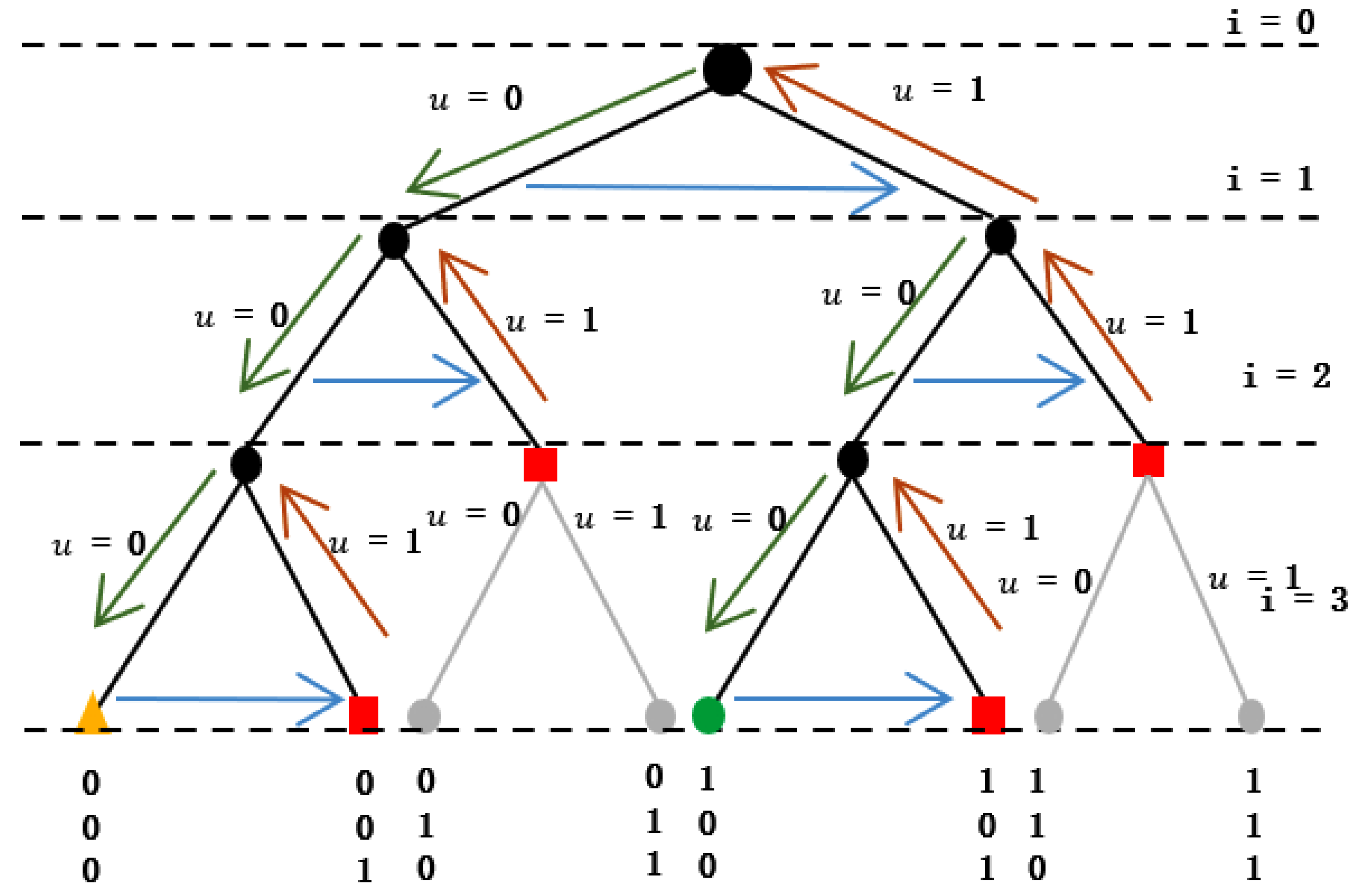
2.4. Sphere Decoding Algorithm Implementation for the PMSM Drive

The challenge in Equation (29), which relates to finding the shortest distance between two vectors, is known as the closest point problem, and several conventional algorithms have already been addressed in [38].

Two algorithms are highlighted, known as the Pohst and Kannan algorithms, with the former using a hypersphere for devising methods regarded as sphere decoders, such as the SDA, although it has been primarily applied in communication theory [39]. Nonetheless, in the context of power electronics, specifically in addressing the long prediction horizon (LPH)-FCS-MPC problem for power converters, a modified sphere decoding algorithm has been developed and adapted [18]; this approach tailors the SDA to suit the requirements of power converter control. This problem can be interpreted as minimizing the hypersphere of radius $\rho$, which corresponds to the value of the cost function, centered at $U_{\mathrm{unc}}\left(k\right)$. The sphere decoding algorithm (SDA) evaluates only those candidate solutions that lie within the computed hypersphere, selecting the one with the smallest cost function as the optimal solution. Specifically, the optimal solution $U^{*}\left(k\right)$ is the n-dimensional lattice point that has the minimum Euclidean distance from the unconstrained solution ${\overline{U}}_{\mathrm{unc}}$, as shown in Figure 5. Equivalently, this solution is the unique lattice point enclosed within the smallest hypersphere centered at ${\overline{U}}_{\mathrm{unc}}$ with radius $\rho$.

A key advantage of SDA is that it ensures optimality with significantly higher computational efficiency compared to the exhaustive enumeration used in Figure 7, coupled with the fact that it does not need to evaluate every possible control input, reducing the exponential computational burden when the prediction horizon is increased. The efficiency of SDA is largely dependent on the initial choice of $\rho$, which must be small enough to minimize the number of evaluated nodes but not too small as to exclude all possible solutions. The initial radius is computed as proposed in [40]:

$$\rho =min\{{\rho }_a,{\rho }_b\},$$

(30)

where

$${\rho }_a={\parallel {\overline{U}}_{\mathrm{unc}}-V{U}_{\mathrm{bab}}\left(k\right)\parallel }^2/,$$

(31)

and

$${\rho }_b={\parallel {\overline{U}}_{\mathrm{unc}}-V{U}_{\mathrm{ed}}\left(k\right)\parallel }^2.$$

(32)

These radii are based on two different approximations: the “Babai estimate” $U_{\mathrm{bab}}$ and the “educational guess” $U_{\mathrm{ed}}$. The Babai estimate represents the rounded, unconstrained solution to the nearest integer vector:

$$U_{\mathrm{bab}}\left(k\right)=\lfloor U_{\mathrm{unc}}\left(k\right)\rceil$$

(33)

whereas the educational guess is given by the previously applied optimal solution $U^{*}(k-1)$ shifted by one time step. Once $U^{*}\left(k\right)$ is determined, following the receding horizon policy, only its first element is applied by the converter, while the remaining elements are discarded. The process then repeats at the next time step over a shifted prediction horizon, incorporating updated measurements and estimates.

After determining the initial radius, the algorithm explores the search tree, evaluating one switching element at a time, effectively reducing the problem to a one-dimensional search at each step. The distance of the first selected element from the unconstrained solution is calculated, and if it falls within the sphere’s boundary, the algorithm proceeds with that branch. Otherwise, the entire branch is discarded, as no further elements from that branch can contribute to a feasible solution within the sphere. This pruning mechanism is fundamental to the SDA and makes it well-suited for long prediction horizons.

Once a feasible solution is found, the radius is recalculated and updated, further refining the search space. This iterative process continues, progressively tightening the sphere’s boundary, thereby eliminating more suboptimal solutions. The final solution obtained at the end of this process is declared optimal.

Figure 8 illustrates the operation of the sphere decoding algorithm for $N_p=1$. At each node in the search tree, the algorithm calculates the cumulative squared deviation up to the current step and then compares it against the squared radius. If the current node’s cost exceeds the radius (yellow triangle), the branch is pruned (grey), and the algorithm backtracks (orange arrow) to explore other nodes. This simplifies the verification process and enhances computational efficiency, ensuring that the sphere decoding algorithm can quickly and effectively prune branches of the search tree that cannot lead to a valid solution within the prescribed radius. When the algorithm reaches a bottom node and finds a candidate solution within the current sphere, it tightens the sphere around this solution. The process is repeated over and over, further tightening the sphere to fewer and fewer candidate solutions, thus refining the search. The SDA terminates when the entire search tree has been explored; only at this point can the algorithm guarantee that the found solution is optimal (green circle), having examined all possible candidate solutions within the defined sphere.

3. Simulation Results and Comparison

In this section, we analyze the impact of the sampling time and a long prediction horizon on the performance of the PMSM, such as the THD of the current, switching frequency, and the effect of the weighing factor ${\lambda }_u$ on the switching frequency. This was also implemented for long predictions of $N_p=3$ and 5.

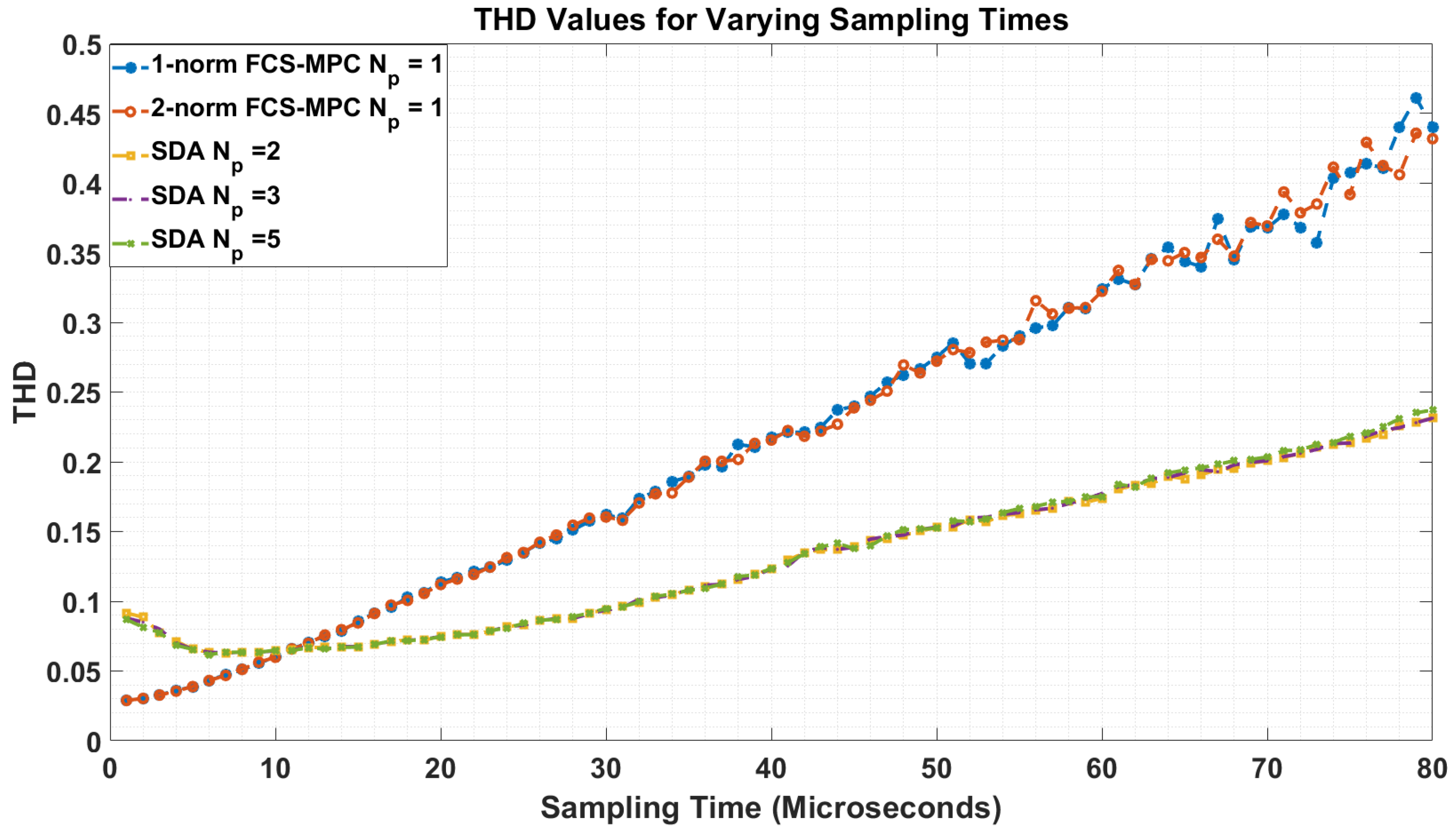
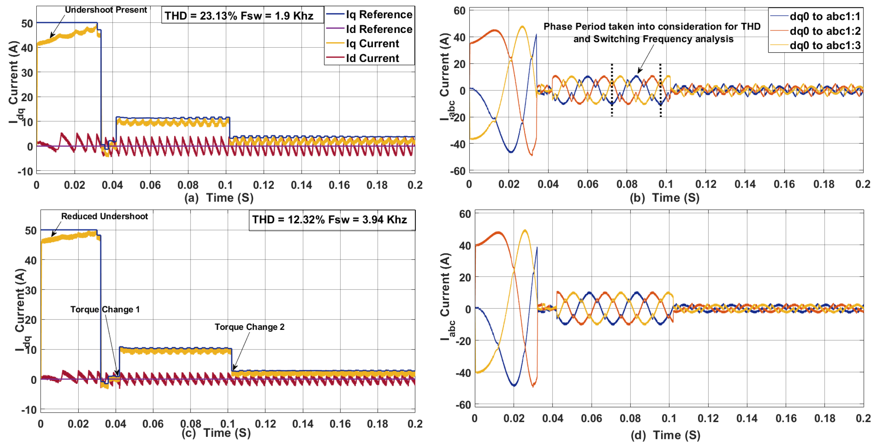
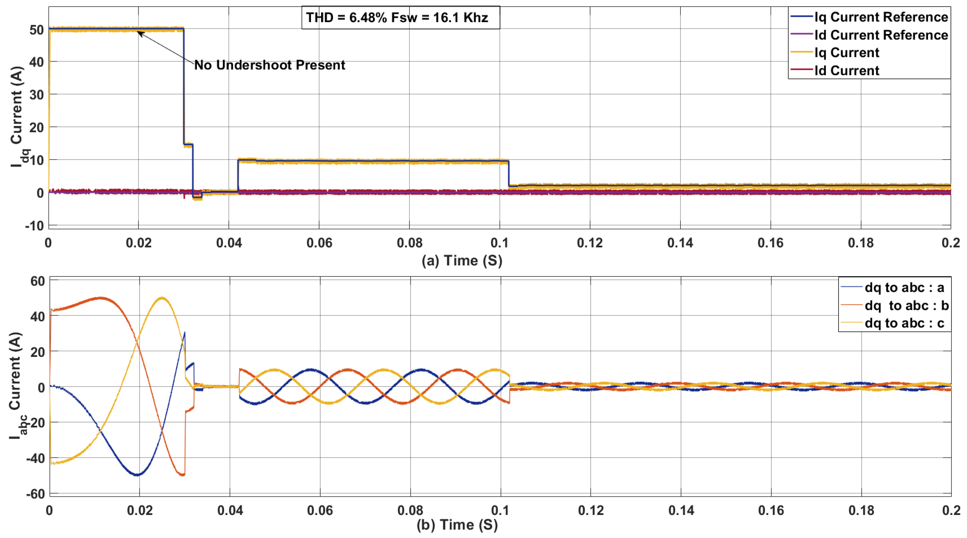
3.1. Effect of Sampling Time on Sphere Decoding Algorithm for PMSM

The SDA algorithm was implemented for a prediction horizon of 2, 3, and 5 over sampling times ranging from 1 to 80 microseconds. Figure 9 shows the trends for FCS-MPC and SDA for various sampling times. This comparison revealed that FCS-MPC outperformed SDA in terms of THD for sampling times less than 10 $\mathsf{\mu }$$\mathrm{s}$. However, for sampling times greater than 10 $\mathsf{\mu }$$\mathrm{s},$ SDA consistently exhibited a lower THD than FCS-MPC, albeit with a significant issue of undershoot, as illustrated in Figure 9.

The SDA introduced in Figure 10 was implemented for a two-step prediction horizon at a sampling time of 40 $\mathsf{\mu }$$\mathrm{s} \mathrm{a}$nd 80 $\mathsf{\mu }$$\mathrm{s}$. It is observed that the undershoot in the current dq-axis becomes more pronounced with higher sampling times, as shown in Figure 10. At 80 $\mathsf{\mu }$s, there is a significant undershoot, with the THD in the current abc-axis being 23.13% and an average switching frequency of 1.9 $\mathrm{KHz}$. However, at a sampling time of 40 $\mathsf{\mu }$$\mathrm{s},$ the undershoot in the dq-axis diminishes but is still present, having a THD of 12.32% in the current abc-axis and an average switching frequency of 3.94 $\mathrm{KHz}$.

To clearly illustrate the impact of load transients on total harmonic distortion (THD) and switching frequency, in Figure 10c, black arrows have been used to denote abrupt torque changes. Specifically, a positive torque step of +10 was introduced at 0.04 s, and a subsequent negative torque step of $-8$ was introduced at 0.1 s. These deliberate disturbances simulate realistic load variations that may occur in aerospace motor operations, yet the methodology remains applicable to a broad range of high-performance drive systems. By emphasizing these transient events, we can effectively evaluate how the control algorithm responds under load changes.

At lower sampling times of (<40 $\mathsf{\mu }$s) $\mathsf{\mu }$$\mathrm{s},$ the undershoot diminishes until it is eliminated at around 10 $\mathsf{\mu }$$\mathrm{s},$ as shown in Figure 11 with a THD of 6.48%; however, it has an average switching frequency of 16.1 $\mathrm{KHz}$. A three-step and five-step prediction horizon was also simulated for the same parameters; the three-step prediction had a THD of 6.28% at an average switching frequency of 17.9 $\mathrm{Khz},$ whereas the five-step SDA had a THD of 6.3% at an average switching frequency of 17.73 $\mathrm{Khz},$ showing that, at maximum switching frequency, the effect of a long prediction horizon is not beneficial in terms of THD reduction. However, the average switching frequency can be controlled when using Equation (10) by tuning the weighing factor ${\lambda }_u$.

3.2. Effect of Weighing Factor ${\lambda }_u$ on THD and Average Switching Frequency $F_{sw}$

In this approach, the value of the weighting factor $\lambda$ was varied from 0.1 to 20 in increments of 0.1, as illustrated in Figure 12. The figure highlights the relationship between the SDA and the FCS-MPC Equation (16) across different $\lambda$ values. A more detailed view of this trend—specifically involving the total harmonic distortion (THD), average switching frequency, and weighting factor—is also presented in Figure 12. The results indicate that increasing the weighting factor reduces the switching frequency but leads to higher THD.

In the comparison shown in Figure 12, each marker point represents a separate simulation run using identical parameters. The simulation corresponding to the highest $\lambda$ value from Figure 12 is further illustrated in Figure 13. In this case, the FCS-MPC shows noticeable instability in the dq- axis and a high THD in the abc- axis. In contrast, the SDA demonstrates a slight undershoot, with an abc- axis THD of 19.8% and an average switching frequency of 3.82 $\mathrm{kHz}$.

3.3. Sphere Decoding Algorithm for $N_p>2$

To show the benefit of the long prediction horizon, a three-step and a five-step prediction horizon SDA was implemented for the same parameter, as shown in Figure 14; there was a decrease in THD from the two to five-step; at the third step, the THD was 16.27% with an average switching frequency of 5.18 $\mathrm{KHz}$. At a prediction horizon of 5, the THD in the abc-axis reduced to 14.49% with an average switching frequency of 5.79 $\mathrm{KHz}$. In this case, the increase in the prediction horizon leads to higher switching frequency and lower THD. To fully assess the impact of the long prediction horizon on system performance, numerous simulations were conducted using the sphere decoding algorithm (SDA) with prediction horizons of two, three, and five steps. These simulations were carried out for different sampling times from 10–80 $\mathsf{\mu }$$\mathrm{s}($eight sampled values).

By extending the prediction horizon, the controller is provided with enhanced foresight over future system states, which can facilitate more effective optimization of switching decisions. This improvement in anticipation is expected to yield a reduction in THD by enabling the controller to better manage and mitigate harmonic distortions in the output waveform. Figure 15 illustrates the comparative results for the two-, three-, and five-step SDA configurations. The red arrow shows the increment of the weighing factor, and the blue arrow shows the increment in sampling time. The simulation outcomes demonstrate that as the prediction horizon is extended, there is a notable decrease in THD, highlighting the benefits of a longer horizon. At the same time, variations in the switching frequency are observed, reflecting the inherent trade-off between achieving lower total harmonic distortion and managing the average switching frequency.

Figure 16 presents the results from a simulation using a randomly selected weighting factor of 10. For the two-step prediction, the THD was 12.98% with an average switching frequency of 6.37 $\mathrm{kHz}$. In the three-step prediction, the THD increased to 13.36%, and the average switching frequency decreased to 5.96 $\mathrm{kHz}$. For the five-step prediction, the THD dropped to 10.64% with a higher average switching frequency of 8.69 $\mathrm{kHz}$. Notably, increasing the prediction horizon from two to three steps resulted in higher THD but a reduction in switching frequency.This highlights the complex and nonlinear relationship between the prediction horizon, switching frequency, and total harmonic distortion (THD). The arrow in the upper three subfigures highlights the decreasing trend of the $I_q$ current ripple.

3.4. Computational Time $N_p>2$

In this section, the computational time of the FCS and SDA is discussed. For the results in

Table 3. Computational time ($\mathsf{\mu }\mathrm{s}$).

Optimization Algorithm	${\mathit{N}}_{\mathit{p}}=1$	${\mathit{N}}_{\mathit{p}}=2$	${\mathit{N}}_{\mathit{p}}=3$	${\mathit{N}}_{\mathit{p}}=5$
FCS-MPC	5.63–16	-	-	-
SDA	4.5–11	46–69	50–57	55–57

, the simulation was run 10 times for each algorithm, and the minimum and maximum values were taken as the range of the algorithm.

The computational time analysis shows that for a short prediction horizon ($N_p=1$), the sphere decoding algorithm (SDA) (4.5–11 $\mathsf{\mu }$$\mathrm{s})$ is more efficient than finite control set model predictive control (FCS-MPC) (5.63–16 $\mathsf{\mu }$$\mathrm{s})$. As shown in Figure 5, this is because SDA does not need to evaluate every possible control sequence, thereby reducing computational burden. In contrast, SDA exhibits a significant increase in computational time from $N_p=1$ to $N_p=2$ (46–69 $\mathsf{\mu }$$\mathrm{s})$. However, beyond this point, the increase stabilizes, with computational time ranging between 50–57 $\mathsf{\mu }$$\mathrm{s} \mathrm{f}$or $N_p=3$ and 55–57 $\mathsf{\mu }$$\mathrm{s} \mathrm{f}$or $N_p=5$. This trend suggests that while SDA initially experiences a sharp rise in computational cost, it becomes more predictable for higher horizons. Since FCS-MPC was not run beyond $N_p=1$, its computational scalability remains uncertain. However, SDA remains feasible even for larger horizons, making it a promising option for computationally constrained applications where extended predictive control is required.

3.5. Effect of Parameter Mismatch on Long Prediction Horizon MPC

In this section, we analyze the impact of parameter mismatches on the performance of the sphere decoding algorithm (SDA) applied to a Permanent Magnet Synchronous Motor (PMSM) drive, paying particular attention to the effect of variations in resistance, inductance, and flux linkage on the system’s total harmonic distortion (THD), switching frequency, and reference current tracking.

3.5.1. Resistance Mismatch

The simulation results demonstrate that variations in the resistance parameter within a reasonable range (e.g., 0.2, 0.5, 5, and 10 times the nominal resistance $R_s$) have a negligible impact on the total harmonic distortion (THD) and the switching frequency of the SDA-based FCS-MPC for PMSM drives. As shown in

Table 4. Resistance parameter mismatch.

Prediction Horizon $\mathsf{\mu }\mathbf{s}$	5 × ${\mathit{R}}_{\mathit{s}}$	0.2 × ${\mathit{R}}_{\mathit{s}}$	10 × ${\mathit{R}}_{\mathit{s}}$
2-Step	12.97 (6.995 $\mathrm{KHz})$	13.01 (7.034 $\mathrm{KHz})$	13.13 (6.97 $\mathrm{KHz})$
3-Step	13.00 (6.545 $\mathrm{KHz})$	12.99 (6.547 $\mathrm{KHz})$	13.38 (6.325 $\mathrm{KHz})$
5-Step	10.15 (9.543 $\mathrm{KHz})$	10.08 (9.543 $\mathrm{KHz})$	10.14 (9.3607 $\mathrm{KHz})$

, regardless of whether the resistance is increased (5 × $R_s$ or 10 × $R_s$) or decreased (0.2 × $R_s$), the THD remains relatively constant, and the corresponding switching frequencies vary slightly.

This minimal influence of resistance mismatch can be primarily attributed to the inherent nature of resistance in PMSM drive systems. Resistance predominantly affects the steady-state voltage drops and the ohmic losses, rather than the dynamic response of the system. Since the SDA-based FCS-MPC controller is designed to dynamically adjust control inputs based on real-time current tracking, it effectively compensates for any deviations in resistance during each control cycle. Consequently, the current waveforms remain consistent, and the phase currents in the abc frame do not exhibit significant distortions.

Furthermore, the structure of the cost function in the FCS-MPC controller primarily optimizes the voltage application to minimize the current error. Since resistance impacts mainly the steady-state power loss and does not alter the system’s dynamic characteristics (such as pole locations), its variations do not lead to substantial differences in the controller’s performance.

3.5.2. Flux Mismatch

Flux linkage mismatch has a relatively minor impact on total harmonic distortion (THD) and switching frequency when compared to inductance mismatch. The THD values remain fairly stable across different flux mismatch conditions, and the switching frequency exhibits little variation, as shown in

Table 5. Flux mismatch.

Prediction Horizon $\mathsf{\mu }\mathbf{s}$	0.1 × ${\mathit{\psi }}_{\mathit{m}}$	0.5 × ${\mathit{\psi }}_{\mathit{m}}$	2 × ${\mathit{\psi }}_{\mathit{m}}$	5 × ${\mathit{\psi }}_{\mathit{m}}$
2-Step	13.05 (6.98 $\mathrm{KHz})$	12.81 (7.0282 $\mathrm{KHz})$	12.69 (7.0051 KHz)	13.07 (7.0355 $\mathrm{KHz})$
3-Step	13.10 (6.585 $\mathrm{KHz})$	13.22 (6.6065 $\mathrm{KHz})$	13.19 (6.5679 $\mathrm{KHz})$	13.13 (6.5767 $\mathrm{KHz})$
5-Step	10.27 (9.4064 $\mathrm{KHz})$	9.97 (9.5314 $\mathrm{KHz})$	9.70 (9.4994 $\mathrm{KHz})$	10.07 (9.4714 $\mathrm{KHz})$

. However, flux mismatch introduces noticeable variations in the reference values of the dq-axis current components, as shown in Figure 17. This behavior can be attributed to the direct influence of flux linkage on the back-electromotive force in the PMSM, which, in turn, affects the generated torque. When the flux linkage is incorrectly estimated, the predictive model used within the SDA-based FCS-MPC either underestimates or overestimates the required voltage commands. Consequently, the computed current references deviate from their ideal values, which may manifest as apparent overshoot or undershoot in the dq current trajectories. Importantly, this perceived overshoot is not indicative of instability; rather, it reflects a shift in the reference due to the flux estimation error. The controller is still capable of tracking these altered references accurately, as the overall dynamic performance of the system remains stable.

Moreover, since flux linkage does not directly affect the motor’s inductive reactance, it does not significantly alter the rate of change of the currents or the system’s time constants. This explains why the switching frequency remains largely unaffected by flux mismatch. The cost function in the FCS-MPC framework focuses on minimizing the error between predicted and actual currents, and any shift in the dq references caused by flux mismatch is dynamically corrected by the controller.

In summary, while flux linkage mismatch may lead to observable shifts in the dq-axis reference values, these shifts do not compromise the stability or overall performance of the control system. The robustness of the SDA-based FCS-MPC against flux mismatch underscores that, within practical limits, the control strategy is more sensitive to dynamic parameters (such as inductance) than to static parameters like flux linkage.

3.5.3. Inductance Mismatch

Inductance mismatch is the most influential parameter affecting the performance of the SDA-based FCS-MPC in PMSM drives, as demonstrated in

Table 6. Inductance parameter mismatch.

Prediction Horizon $\mathsf{\mu }\mathbf{s}$	0.1 × ${\mathit{L}}_{\mathbf{dq}}$	0.5 × ${\mathit{L}}_{\mathbf{dq}}$	2 × ${\mathit{L}}_{\mathbf{dq}}$	5 × ${\mathit{L}}_{\mathbf{dq}}$
2-Step	29.72 (1.58 $\mathrm{KHz})$	12.85 (8.4147 $\mathrm{KHz})$	18.37 (4.4052 KHz)	39.60 (3.108 KHz)
3-Step	29.67 (1.62 $\mathrm{KHz})$	11.20 (10.448 $\mathrm{KHz})$	12.48 (7.0995 KHz)	22.22 (4.3292 $\mathrm{KHz})$
5-Step	29.37 (1.6717 $\mathrm{KHz})$	9.57 (13.647 $\mathrm{KHz})$	13.20 (7.0751 $\mathrm{KHz})$	12.09 (7.3826 $\mathrm{KHz})$

. When the inductance is drastically underestimated (e.g., $0.1\times L_{dq}$), the controller exhibits very high THD values, around 29–30%, across all prediction horizons with a correspondingly low switching frequency of approximately 1.6 $\mathrm{KHz}$. This behavior indicates that an underestimation of inductance drastically reduces the motor’s electrical time constant, $\tau ={\displaystyle \frac{L}{R}}$, causing the current to change too abruptly in response to voltage variations. Consequently, the voltage vectors selected by the controller fail to correct these rapid changes, resulting in a distorted current waveform with high THD and minimal corrective switching.

Conversely, when the inductance is moderately underestimated (e.g., $0.5\times L_{dq}$), the performance improves significantly. For a two-step prediction, the THD drops to 12.85% with an increased switching frequency of about 8.4 $\mathrm{KHz};$ further improvements are observed in the three-step and five-step predictions, with THD values decreasing to 11.20% and 9.57%, respectively. However, this improvement comes at the cost of an increased switching frequency, reflecting a more aggressive corrective action as the controller compensates for the residual mismatch. This compensation is indicative of the controller’s attempt to maintain current tracking despite an imperfect model.

When the inductance is overestimated (e.g., $2\times L_{dq}$), the effects vary with the prediction horizon. For a two-step prediction, the THD increases to 18.37% with a lower switching frequency of 4.41 $\mathrm{KHz},$ implying that the controller is undercompensating for the slower response induced by the higher inductance. In contrast, for the three-step and five-step predictions, the THD improves to 12.48% and 13.20%, with switching frequencies around 7.10 $\mathrm{KHz},$ indicating that longer prediction horizons can partially mitigate the adverse effects of an overestimated inductance by providing better foresight into system dynamics.

In the case of extreme overestimation (e.g., $5\times L_{dq}$), performance deteriorates markedly for shorter prediction horizons; a two-step prediction yields a very high THD of 39.60% with a low switching frequency of 3.11 $\mathrm{KHz},$ while a three-step prediction shows a THD of 22.22% at 4.33 $\mathrm{KHz}$. Interestingly, the five-step prediction in this scenario achieves a much improved THD of 12.09% with a switching frequency of 7.38 $\mathrm{KHz},$ suggesting that extended prediction horizons can partially compensate for the mismatch by aligning control actions with the slower system response.

From a theoretical perspective, these observations are well explained by control theory. The electrical time constant, $\tau ={\displaystyle \frac{L}{R}}$, is critical in determining the system’s dynamic response. A lower L results in a shorter $\tau$, causing faster but more volatile current changes, whereas a higher L increases $\tau$, leading to a sluggish response that the controller attempts to counterbalance with increased switching. In the closed-loop transfer function of the current control loop, the pole positions are directly influenced by L; significant deviations in L alter these poles, resulting in either overly aggressive or insufficient corrective actions. Therefore, the controller’s performance is highly sensitive to the accuracy of the inductance parameter.

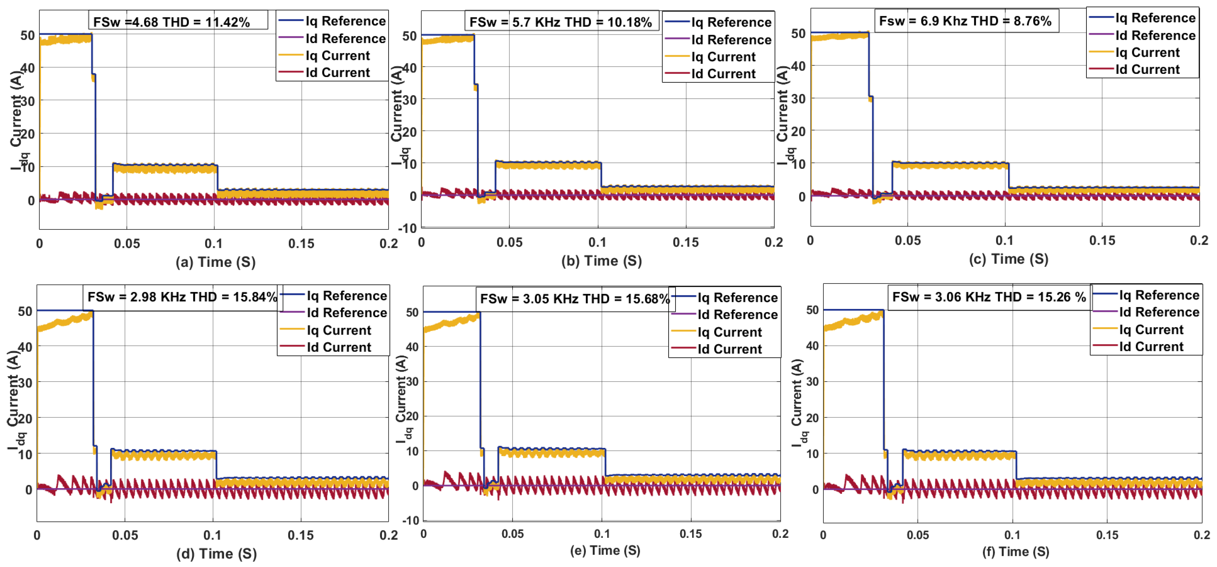
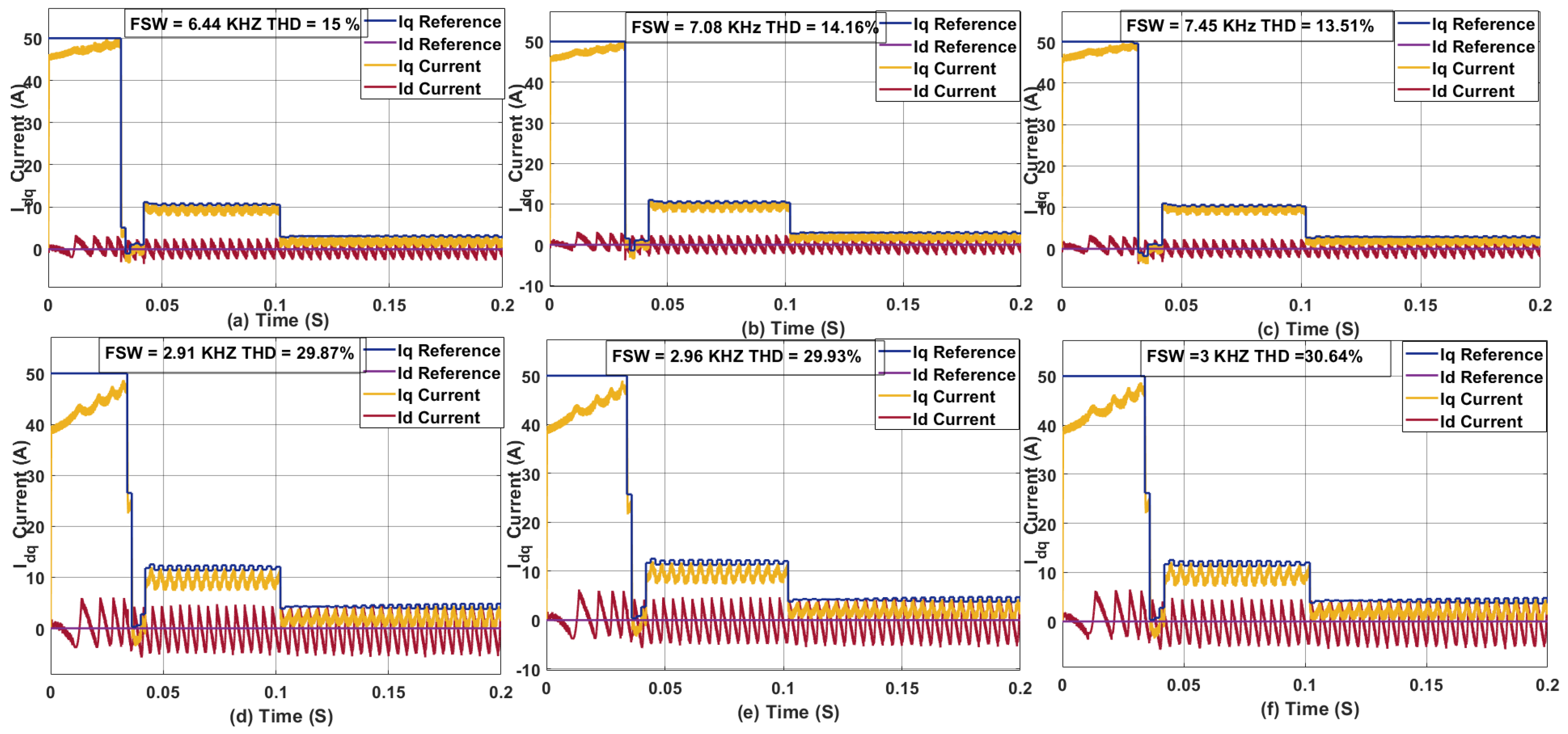
3.6. Effect of Nonlinear Inductance on SDA for PMSM

In actual applications, the inductance of a PMSM is nonlinear, varying with operating conditions such as temperature, saturation, and current amplitude [41]. To emulate this nonlinearity, a step change of +50% in inductance was introduced mid-simulation at 0.07 s. Unlike the earlier approach, where the inductance mismatch was applied from the start, this method better reflects the time-varying and nonlinear behavior observed in real machines. The test was carried out for sampling times of 10 $\mathsf{\mu }$s and 50 $\mathsf{\mu }$s. In Figure 18a–c, with a sampling time of 10 $\mathsf{\mu }$s, introducing the mismatch at 0.07 s led to an increase in THD from 13.03% to 19.73% in the two-step prediction case, along with a slight rise in switching frequency. For the three-step prediction, THD slightly decreased from 13.39% to 12.77%, also accompanied by a rise in switching frequency. In the five-step case, THD increased, similar to the two-step result, with a marginal increase in switching frequency. In Figure 18d–f, for a sampling time of 50 $\mathsf{\mu }$s, the impact of inductance mismatch was notably different. In the two-step prediction, THD dropped from 16.65% to 9.25% with a slight rise in switching frequency. The three-step and five-step cases also showed THD reductions from 16.61% to 8.87% and from 16.15% to 8.8%, respectively, again with slight increases in switching frequency. These results suggest that the +50% inductance mismatch appears to benefit SDA-MPC performance under larger sampling times, likely due to the extended prediction horizon compensating for modeling inaccuracies.

In Figure 19a–c, when a −50% inductance mismatch is introduced at 0.07 s, the two-step prediction case shows a decrease in THD from 13.03% to 12.74%, with an increase in switching frequency. For the three-step prediction, THD drops from 13.39% to 11.35%, and in the five-step case, from 10.45% to 9.57%, both with increased switching frequencies. These results indicate that at a low sampling time of 10 $\mathsf{\mu }$s, the −50% inductance mismatch is beneficial for both THD and switching performance. In contrast, Figure 19d–f presents the results at a 50 $\mathsf{\mu }$s sampling time. Here, all three prediction horizons exhibit significant degradation. The two-step prediction shows an increase in THD from 16.65% to 29.15%, the three-step from 16.61% to 29.17%, and the five-step from 16.15% to 29.69%, all accompanied by rises in switching frequency. This indicates that negative inductance mismatch at higher sampling times substantially deteriorates current quality.

3.7. Coupled Effect of Sampling Time, Control Effort, and Inductance Mismatch on the PMSM Drive

While the previous subsections investigated the impact of sampling time, control effort weighting, and parameter mismatch independently, real-world conditions often involve simultaneous deviations across multiple factors. In this subsection, the combined effect of these three variables on the performance of the MPC framework was applied to a PMSM by choosing two sampling times, a weighting factor, and parameter mismatch.

Figure 20 compares the performance under no parameter mismatch for two sampling times (20 $\mathsf{\mu }$$\mathrm{s} \mathrm{a}$nd 50 $\mathsf{\mu }$$\mathrm{s})$, across different prediction horizons (two, three, and five steps) and control effort weightings. Subfigures (a–c) show the results for a fast sampling time of 20 $\mathsf{\mu }$$\mathrm{s} \mathrm{w}$ith ${\lambda }_u=7$, while (d–f) represent 50 $\mathsf{\mu }$$\mathrm{s} \mathrm{w}$ith ${\lambda }_u=3$. As the horizon increases in (a–c), the initial undershoot diminishes due to improved predictive capability, with a concurrent reduction in THD and rise in switching frequency. In contrast, for the 50 $\mathsf{\mu }$$\mathrm{s} \mathrm{c}$ases (d–f), undershoot persists, despite increasing horizon length, and both THD and switching frequency exhibit only marginal improvements.

Figure 21 illustrates the system behavior under −50% in inductance, comparing performance across prediction horizons and two sampling rates. In the top row (a–c), where the sampling time is 20 $\mathsf{\mu }$$\mathrm{s},$ an undershoot is observed in the Iq response for the two-step case, likely due to the controller’s incorrect prediction of system dynamics. With increasing steps, the undershoot remains, and THD reduces slightly, but the overall THD values and switching frequency remain higher than in the no-mismatch case. Notably, switching frequencies increase as the controller compensates for prediction inaccuracies by adjusting its decisions more aggressively. In contrast, the bottom row (d–f) shows degraded performance at a 50 $\mathsf{\mu }$$\mathrm{s} \mathrm{s}$ampling interval. Here, undershoot persists, and THD unexpectedly increases with prediction step, indicating that longer prediction under poor model accuracy and slower updates amplifies the control error. These findings highlight the limitations of standard MPC under model mismatch and emphasize the need for model adaptation or online identification.

Figure 22a–c present results under a +50% inductance mismatch, which exhibited noticeably lower switching frequency with slightly higher THD compared to the no-mismatch cases in Figure 20a–c, with the five-step prediction in Figure 20c having a slightly lower THD and a noticeably lower switching frequency than Figure 20c. For Figure 22d–f, the increase in steps lower the THD by a slight amount. However, when benchmarked against the corresponding no-mismatch cases in Figure 20d–f, these mismatched conditions demonstrate improved performance in both THD and switching frequency.

4. Conclusions

In this paper, we investigated the performance of a sphere decoding algorithm (SDA)-based finite control set model predictive control (FCS-MPC) for PMSM drives, with a particular focus on the effects of sampling time, control effort weighting, and parameter mismatches. Our simulation results demonstrate that at longer sampling times (40 and 80 $\mathsf{\mu }$$\mathrm{s})$, significant undershoot occurs in the current response. As the sampling time is reduced below 40 $\mathsf{\mu }$$\mathrm{s},$ the undershoot gradually diminishes and disappears entirely at a 10 $\mathsf{\mu }$$\mathrm{s} \mathrm{s}$ampling time. At this shorter sampling time, while the inclusion of a control effort term successfully reduces the switching frequency, a small undershoot remains, indicating that the predicted output closely follows the reference but does not perfectly align with the midpoint of the desired waveform. Furthermore, our investigation into parameter mismatches revealed that variations in resistance and flux linkage have a negligible effect on the system’s THD and switching frequency. In contrast, inductance mismatches significantly impact the controller’s performance. Depending on the magnitude of the inductance error, the system sometimes compensates by increasing the switching frequency; however, for severe mismatches, the system can become unstable. This outcome underscores the critical importance of accurate inductance estimation in ensuring effective current tracking and maintaining low THD. From an aerospace perspective, achieving low torque ripple and high efficiency is paramount for PMSM applications in electric propulsion and actuation systems. The findings suggest that optimizing the prediction horizon and control effort weighting can significantly improve dynamic performance, reducing electromagnetic interference and enhancing system reliability in aircraft environments where precise control is essential.

The SDA-MPC method for PMSM control offers several advantages over conventional MPC approaches. One key benefit is its ability to reduce the computational burden as the prediction horizon increases due to the efficiency of the sphere decoding algorithm, which avoids exhaustive evaluation of all possible voltage vectors, as shown in Figure 5. It also enables implicit control of the switching frequency through appropriate tuning of the control effort weighting ${\lambda }_u$. The method has also shown improved current quality, particularly in terms of reduced total harmonic distortion (THD), when compared to traditional MPC schemes. However, the SDA method also has some limitations. Its performance is highly dependent on the sampling time; lower sampling times (e.g., 10–20 $\mathsf{\mu }$s) are necessary to maintain good dynamic response and low THD, while higher sampling times result in noticeable degradation. Lastly, the computational requirements of the method may be challenging for low-end hardware platforms, especially when very fast sampling is required.

Looking ahead, future research should focus on enhancing the robustness of the SDA-based FCS-MPC approach in the presence of parameter mismatches. One promising direction is the integration of Recursive Least Squares (RLS) for real-time parameter estimation. RLS can continuously update key parameters such as resistance, inductance, and flux linkage, mitigating the adverse effects of mismatches and enabling the controller to maintain optimal performance, despite variations due to temperature, aging, or manufacturing tolerances. Additionally, exploring hybrid adaptive estimation methods, such as combining RLS with an Extended Kalman Filter, may further improve noise rejection and estimation accuracy. Experimental validation on a physical PMSM setup under various operating conditions, including thermal and load variations, will be sought in future studies to confirm the practical viability of the proposed solutions in aerospace applications.

References

1. Weimer, J. Electrical power technology for the more electric aircraft. In Proceedings of the [1993 Proceedings] AIAA/IEEE Digital Avionics Systems Conference, Fort Worth, TX, USA, 25 October 2005–28 October 1993; pp. 445–450. [Google Scholar]
2. Liao, C.; Bianchi, N.; Zhang, Z. Recent Developments and Trends in High-Performance PMSM for Aeronautical Applications. Energies 2024, 17, 6199. [Google Scholar] [CrossRef]
3. Finken, T.; Felden, M.; Hameyer, K. Comparison and design of different electrical machine types regarding their applicability in hybrid electrical vehicles. In Proceedings of the 2008 18th International Conference on Electrical Machines, Vilamoura, Portugal, 6–9 September 2008; pp. 1–5. [Google Scholar] [CrossRef]
4. Ford, A. Brushless generators for aircraft—A review of current developments. Proc. IEE Part A Power Eng. 1962, 109, 437–452. [Google Scholar] [CrossRef]
5. Pardo-Vicente, M.A.; Guerrero, J.M.; Platero, C.A.; Sánchez-Férnandez, J.A. Contactless Rotor Ground Fault Detection Method for Brushless Synchronous Machines Based on an AC/DC Rotating Current Sensor. Sensors 2023, 23, 9065. [Google Scholar] [CrossRef] [PubMed]
6. Strobl, S. Field Oriented Control (FOC) of Permanent Magnet Synchronous Machine (PMSM). 2021. Available online: https://imperix.com/doc/implementation/field-oriented-control-of-pmsm (accessed on 28 March 2024).
7. Aguilera, R.P.; Acuna, P.; Konstantinou, G.; Vazquez, S.; Leon, J.I. Chapter 2—Basic Control Principles in Power Electronics: Analog and Digital Control Design. In Control of Power Electronic Converters and Systems; Blaabjerg, F., Ed.; Academic Press: Cambridge, MA, USA, 2018; pp. 31–68. [Google Scholar] [CrossRef]
8. Zhang, Z.; Dragicevic, T.; Li, Y.; Wang, Y.; Zheng, C.; Leng, M.; Rodriguez, J. Chapter 4–Model predictive control of power converters, motor drives, and microgrids. In Control of Power Electronic Converters and Systems; Blaabjerg, F., Ed.; Academic Press: Cambridge, MA, USA, 2021; pp. 101–124. [Google Scholar] [CrossRef]
9. Rodriguez, J.; Pontt, J.; Silva, C.A.; Correa, P.; Lezana, P.; Cortes, P.; Ammann, U. Predictive Current Control of a Voltage Source Inverter. IEEE Trans. Ind. Electron. 2007, 54, 495–503. [Google Scholar] [CrossRef]
10. Matias Aguirre, M.; Vazquez, S.; Wilson-Veas, A.H.; Kouro, S.; Rojas, C.A.; Leon, J.I.; Franquelo, L.G. Extended Period Control Approach FCS-MPC for Three Phase NPC Power Converters. IEEE Trans. Power Electron. 2025, 40, 4927–4937. [Google Scholar] [CrossRef]
11. Vazquez, S.; Rodriguez, J.; Rivera, M.; Franquelo, L.G.; Norambuena, M. Model Predictive Control for Power Converters and Drives: Advances and Trends. IEEE Trans. Ind. Electron. 2017, 64, 935–947. [Google Scholar] [CrossRef]
12. Gade, C.R.; W, R.S. Control of Permanent Magnet Synchronous Motor Using MPC–MTPA Control for Deployment in Electric Tractor. Sustainability 2022, 14, 12428. [Google Scholar] [CrossRef]
13. Murali, A.; Wahab, R.S.; Gade, C.S.R.; Annamalai, C.; Subramaniam, U. Assessing Finite Control Set Model Predictive Speed Controlled PMSM Performance for Deployment in Electric Vehicles. World Electr. Veh. J. 2021, 12, 41. [Google Scholar] [CrossRef]
14. Li, X.; Yang, Q.; Tian, W.; Karamanakos, P.; Kennel, R. A Dual Reference Frame Multistep Direct Model Predictive Current Control With a Disturbance Observer for SPMSM Drives. IEEE Trans. Power Electron. 2022, 37, 2857–2869. [Google Scholar] [CrossRef]
15. Dorfling, T.; Mouton, H.; Geyer, T.; Karamanakos, P. Long-Horizon Finite-Control-Set Model Predictive Control With Nonrecursive Sphere Decoding on an FPGA. IEEE Trans. Power Electron. 2019, 69, 7520–7531. [Google Scholar] [CrossRef]
16. Karamanakos, P.; Geyer, T. Guidelines for the Design of Finite Control Set Model Predictive Controllers. IEEE Trans. Power Electron. 2020, 35, 7434–7450. [Google Scholar] [CrossRef]
17. Zafra, E.; Granado, J.; Lecuyer, V.B.; Vazquez, S.; Alcaide, A.M.; Leon, J.I.; Franquelo, L.G. Computationally Efficient Sphere Decoding Algorithm Based on Artificial Neural Networks for Long-Horizon FCS-MPC. IEEE Trans. Ind. Electron. 2024, 71, 39–48. [Google Scholar] [CrossRef]
18. Geyer, T.; Quevedo, D.E. Multistep Finite Control Set Model Predictive Control for Power Electronics. IEEE Trans. Power Electron. 2014, 29, 6836–6846. [Google Scholar] [CrossRef]
19. Zafra, E.; Vazquez, S.; Alcaide, A.M.; Franquelo, L.; Leon, J.; Pérez, E. K-Best Sphere Decoding Algorithm for Long Prediction Horizon FCS-MPC. IEEE Trans. Ind. Electron. 2021, 69, 7571–7581. [Google Scholar] [CrossRef]
20. Akinwumi, J.O.; Gao, Y.; West, G.T.; Ruiz, H.S. Optimisation Algorithms in Multi-Step Prediction Horizon MPC for Two-Level Inverters. In Proceedings of the 2024 International Symposium on Electrical, Electronics and Information Engineering (ISEEIE), Leicester, UK, 26–28 September 2024; pp. 115–122. [Google Scholar] [CrossRef]
21. Lin, C.K.; Liu, T.H.; Yu, J.t.; Fu, L.C.; Hsiao, C.F. Model-Free Predictive Current Control for Interior Permanent-Magnet Synchronous Motor Drives Based on Current Difference Detection Technique. IEEE Trans. Ind. Electron. 2014, 61, 667–681. [Google Scholar] [CrossRef]
22. Lin, C.K.; Yu, J.t.; Lai, Y.S.; Yu, H.C. Improved Model-Free Predictive Current Control for Synchronous Reluctance Motor Drives. IEEE Trans. Ind. Electron. 2016, 63, 3942–3953. [Google Scholar] [CrossRef]
23. Yuan, X.; Zhang, S.; Zhang, C. Improved Model Predictive Current Control for SPMSM Drives with Parameter Mismatch. IEEE Trans. Ind. Electron. 2019, 67, 852–862. [Google Scholar] [CrossRef]
24. Ortombina, L.; Karamanakos, P.; Zigliotto, M. Robustness Analysis of Long-Horizon Direct Model Predictive Control: Permanent Magnet Synchronous Motor Drives. In Proceedings of the 2020 IEEE 21st Workshop on Control and Modeling for Power Electronics (COMPEL), Aalborg, Denmark, 9–12 November 2020; pp. 1–8. [Google Scholar] [CrossRef]
25. Geyer, T.; Quevedo, D.E. Multistep direct model predictive control for power electronics — Part 2: Analysis. In Proceedings of the 2013 IEEE Energy Conversion Congress and Exposition, Denver, CO, USA, 15–19 September 2013; pp. 1162–1169. [Google Scholar] [CrossRef]
26. Zhang, X.; Zhao, Z. Multi-Stage Series Model Predictive Control for PMSM Drives. IEEE Trans. Veh. Technol. 2021, 70, 6591–6600. [Google Scholar] [CrossRef]
27. Jeong, I.; Hyon, B.J.; Nam, K. Dynamic Modeling and Control for SPMSMs With Internal Turn Short Fault. IEEE Trans. Power Electron. 2013, 28, 3495–3508. [Google Scholar] [CrossRef]
28. Wang, Y.; Zhu, J.; Wang, S.; Guo, Y.; Xu, W. Nonlinear Magnetic Model of Surface Mounted PM Machines Incorporating Saturation Saliency. IEEE Trans. Magn. 2009, 45, 4684–4687. [Google Scholar] [CrossRef]
29. Mohamed, I.S.; Rovetta, S.; Do, T.D.; Dragicevic, T.; Diab, A.A.Z. A Neural-Network-Based Model Predictive Control of Three-Phase Inverter With an Output LC Filter. IEEE Access 2019, 7, 124737–124749. [Google Scholar] [CrossRef]
30. Bi, E.; Yang, J.; Liu, Y.; Wang, X. Multistep finite-control-set model predictive control of active power filter. IOP Conf. Ser. Earth Environ. Sci. 2020, 617, 012039. [Google Scholar] [CrossRef]
31. Xia, C.; Liu, T.; Shi, T.; Song, Z. A Simplified Finite-Control-Set Model-Predictive Control for Power Converters. IEEE Trans. Ind. Inform. 2014, 10, 991–1002. [Google Scholar] [CrossRef]
32. Narimani, M.; Wu, B.; Yaramasu, V.; Cheng, Z.; Zargari, N.R. Finite Control-Set Model Predictive Control (FCS-MPC) of Nested Neutral Point-Clamped (NNPC) Converter. IEEE Trans. Power Electron. 2015, 30, 7262–7269. [Google Scholar] [CrossRef]
33. Karamanakos, P.; Geyer, T.; Kennel, R. On the Choice of Norm in Finite Control Set Model Predictive Control. IEEE Trans. Power Electron. 2018, 33, 7105–7117. [Google Scholar] [CrossRef]
34. Zheng, C.; Dragicevic, T.; Blaabjerg, F. Current-Sensorless Finite-Set Model Predictive Control for LC-Filtered Voltage Source Inverters. IEEE Trans. Power Electron. 2020, 35, 1086–1095. [Google Scholar] [CrossRef]
35. Kouro, S.; Cortes, P.; Vargas, R.; Ammann, U.; Rodriguez, J. Model Predictive Control—A Simple and Powerful Method to Control Power Converters. IEEE Trans. Ind. Electron. 2009, 56, 1826–1838. [Google Scholar] [CrossRef]
36. Geyer, T. Model Predictive Control of High Power Convertersand Industrial Drives; John Wiley & Sons, Ltd.: Hoboken, NJ, USA, 2016; pp. 1–545. [Google Scholar] [CrossRef]
37. Acuna, P.; Rojas, C.A.; Baidya, R.; Aguilera, R.P.; Fletcher, J.E. On the Impact of Transients on Multistep Model Predictive Control for Medium-Voltage Drives. IEEE Trans. Power Electron. 2019, 34, 8342–8355. [Google Scholar] [CrossRef]
38. Agrell, E.; Eriksson, T.; Vardy, A.; Zeger, K. Closest point search in lattices. IEEE Trans. Inf. Theory 2002, 48, 2201–2214. [Google Scholar] [CrossRef]
39. Zafra, E.; Vazquez, S.; Geyer, T.; Aguilera, R.P.; Franquelo, L.G. Long Prediction Horizon FCS-MPC for Power Converters and Drives. IEEE Open J. Ind. Electron. Soc. 2023, 4, 159–175. [Google Scholar] [CrossRef]
40. Karamanakos, P.; Geyer, T.; Kennel, R. Suboptimal search strategies with bounded computational complexity to solve long-horizon direct model predictive control problems. In Proceedings of the 2015 IEEE Energy Conversion Congress and Exposition (ECCE), Montreal, QC, Canada, 20–24 September 2015; pp. 334–341. [Google Scholar] [CrossRef]
41. Luo, G.; Zhang, R.; Chen, Z.; Tu, W.; Zhang, S.; Kennel, R. A Novel Nonlinear Modeling Method for Permanent-Magnet Synchronous Motors. IEEE Trans. Ind. Electron. 2016, 63, 6490–6498. [Google Scholar] [CrossRef]
Figure 1. Different control methods for motor drives.
Aerospace 12 00458 g001
Figure 2. Categories of MPC.
Aerospace 12 00458 g002
Figure 3. Different aspects of MPC.
Aerospace 12 00458 g003
Figure 4. Illustration of FCS-MPC for PMSM drive.
Aerospace 12 00458 g004
Figure 5. Visualization of FCS-MPC problem with N p = 1 in the original abc-axis; the unconstrained solution is shown in red, the suboptimal solution is shown in yellow, the optimal solution is shown in green, the remaining solutions are shown in blue.
Aerospace 12 00458 g005
Figure 6. Illustration of sphere decoding algorithm for PMSM drive.
Aerospace 12 00458 g006
Figure 7. Visualization of the FCS-MPC problem with N p = 1 in the abc plane, transformed by generator matrix V. the unconstrained solution is shown in red, the suboptimal solution is shown in yellow, the optimal solution is shown in green, the remaining solutions are shown in blue. The solid black circle represents the computed hypersphere in which lies the optimal solution.
Aerospace 12 00458 g007
Figure 8. One- step horizon search tree for a three-phase, two-level inverter explored by the SDA algorithm. The blue arrows indicate side tracking, the orange arrows indicate backtracking, and the green arrows indicate the depth of the first search progressing to the bottom layer.The Current incumbent solution (yellow triangle), the uexplored/pruned branch (grey), teminated node(red), green circle (optimal solution).
Aerospace 12 00458 g008
Figure 9. THD for various sampling times for FCS-MPC and SDA with λ u = 5 × 10 6 .
Aerospace 12 00458 g009
Figure 10. (a) Current in the dq-axis for T s = 80 μ s   w ith λ u = 5 × 10 6 . (b) Current in the abc-axis for T s = 80 μ s. (c) Current in the dq-axis for T s = 40 μ s s   w ith λ u = 5 × 10 6 . (d) Current in the abc-axis for T s = 40 μ s.
Aerospace 12 00458 g010
Figure 11. (a) The dq- axis current for two SDAs with λ u = 5 × 10 6 for T s = 10 μ s . (b) The abc-axis current for two SDAs with λ u = 5 × 10 6 for T s = 10 μ s .
Aerospace 12 00458 g011
Figure 12. Effect of weighing factor on FCS-MPC with 2-norm and SDA with N P = 2 .
Aerospace 12 00458 g012
Figure 13. (a) Current in the dq-axis for T s = 10 μ s   w ith λ u = 20 for a single-step FCS-MPC with 2-norm. (b) Current in the abc-axis for T s = 10 μ s   w ith λ u = 20 for a single-step FCS-MPC with 2-norm. (c) Current in the dq-axis for T s = 10 μ s with λ u = 20 for a two-step SDA. (d) Current in the abc-axis for T s = 10 μ s with λ u = 20 for a two-step SDA.
Aerospace 12 00458 g013
Figure 14. (a) Current in the dq-axis for T s = 10 μ s   w ith λ u = 20 for a three-step SDA. (b) Current in the abc-axis for T s = 10 μ s   w ith λ u = 20 for a three-step SDA. (c) Current in the dq-axis for T s = 10 μ s   w ith λ u = 20 for a five-step SDA. (d) Current in the abc-axis for T s = 10 μ s   w ith λ u = 20 for a five-step SDA.
Aerospace 12 00458 g014
Figure 15. (a) Top and bottom figure (left): Effect of sampling time and weighing factor on a two-step prediction SDA, THD, and average switching frequency. (b) Top and bottom figure (Middle): Effect of sampling time and weighing factor effect on a three-step prediction SDA THD and average switching frequency. (c) Effect of sampling time and weighing factor effect on a five-step prediction SDA THD and average switching frequency.
Aerospace 12 00458 g015
Figure 16. (a) Current in the dq-axis for T s = 10 μ s   w ith λ u = 10 for a two-step SDA. (b) Current in the abc-axis for T s = 10 μ s   w ith λ u = 10 for a two-step SDA. (c) Current in the dq-axis for T s = 10 μ s   w ith λ u = 10 for a three-step SDA. (d) Current in the abc-axis for 10 μ s   w ith λ u = 10 for a three-step SDA. (e) Current in the dq-axis for T s = 10 μ s   w ith λ u = 10 for a five-step SDA. (f) Current in the abc-axis for T s = 10 μ s with λ u = 10 for a five-step SDA.
Aerospace 12 00458 g016
Figure 17. (a) Current in the dq-axis for T s = 10 μ s   w ith λ u = 20 for a two-step SDA with paramter mismatch 0.1 × ψ . (b) Current in the dq-axis for T s = 10 μ s   w ith λ u = 20 for a two-step SDA with paramter mismatch 5 × ψ .
Aerospace 12 00458 g017
Figure 18. Simulation results with inductance change at 0.07 s. (a) Current in the dq-axis for T s = 10 μ s with λ u = 10 for a two-step SDA with + 50% inductance mismatch. (b) Current in the dq-axis for T s = 10 μ s with λ u = 10 for a three-step SDA with + 50% inductance mismatch. (c) Current in the dq-axis for T s = 10 μ s   w ith λ u = 10 for a five-step SDA with + 50% inductance mismatch. (d) Current in the dq-axis for 50 μ s   w ith λ u = 3 for a two-step SDA with + 50% inductance mismatch. (e) Current in the dq-axis for T s = 50 μ s   w ith λ u = 3 for a three-step SDA with + 50% inductance mismatch. (f) Current in the dq-axis for T s = 50 μ s   w ith λ u = 3 for a five-step SDA with + 50% inductance mismatch.
Aerospace 12 00458 g018
Figure 19. (a) Current in the dq-axis for T s = 10 μ s   w ith λ u = 10 for a two-step SDA with −50% inductance mismatch. (b) Current in the dq-axis for T s = 10 μ s   w ith λ u = 10 for a three-step SDA with −50% inductance mismatch. (c) Current in the dq-axis for T s = 10 μ s   w ith λ u = 10 for a five-step SDA with −50% inductance mismatch. (d) Current in the dq-axis for 50 μ s   w ith λ u = 3 for a two-step SDA with −50% inductance mismatch. (e) Current in the dq-axis for T s = 50 μ s   w ith λ u = 3 for a three-step SDA with −50% inductance mismatch. (f) Current in the dq-axis for T s = 50 μ s   w ith λ u = 3 for a five-step SDA with −50% inductance mismatch.
Aerospace 12 00458 g019
Figure 20. (a) Current in the dq-axis for T s = 20 μ s   w ith λ u = 7 for a two-step SDA with no inductance mismatch. (b) Current in the dq-axis for T s = 20 μ s   w ith λ u = 7 for a three-step SDA with no inductance mismatch. (c) Current in the dq-axis for T s = 20 μ s   w ith λ u = 7 for a five-step SDA with no inductance mismatch. (d) Current in the dq-axis for 50 μ s   w ith λ u = 3 for a two-step SDA. (e) Current in the dq-axis for T s = 50 μ s   w ith λ u = 3 for a three-step SDA with no inductance mismatch. (f) Current in the dq-axis for T s = 50 μ s   w ith λ u = 3 for a five-step SDA with no inductance mismatch.
Aerospace 12 00458 g020
Figure 21. (a) Current in the dq-axis for T s = 20 μ s   w ith λ u = 7 for a two-step SDA with −50% inductance mismatch. (b) Current in the dq-axis for T s = 20 μ s   w ith λ u = 7 for a three-step SDA with −50% mismatch. (c) Current in the dq-axis for T s = 20 μ s   w ith λ u = 7 for a five-step SDA with −50% mismatch. (d) Current in the dq-axis for 50 μ s   w ith λ u = 3 for a two-step SDA with −50% inductance mismatch. (e) Current in the dq-axis for T s = 50 μ s   w ith λ u = 3 for a three-step SDA with −50% inductance. mismatch. (f) Current in the dq-axis for T s = 50 μ s   w ith λ u = 3 for a five-step SDA with −50% inductance mismatch.
Aerospace 12 00458 g021
Figure 22. (a) Current in the dq-axis for T s = 20 μ s   w ith λ u = 7 for a two-step SDA +50% inductance mismatch. (b) Current in the dq-axis for T s = 20 μ s   w ith λ u = 7 for a two-step SDA +50% inductance mismatch. (c) Current in the dq-axis for T s = 20 μ s   w ith λ u = 7 for a three-step SDA +50% inductance mismatch. (d) Current in the dq-axis for 50 μ s   w ith λ u = 3 for a three-step SDA +50% inductance mismatch. (e) Current in the dq-axis for T s = 50 μ s   w ith λ u = 3 for a five-step SDA +50% inductance mismatch. (f) Current in the dq-axis for T s = 50 μ s   w ith λ u = 3 for a five-step SDA +50% inductance mismatch.
Aerospace 12 00458 g022