The Calculation and Optimization Methodology of Repairable Elements of a UAV Structure

Abstract

A novel approach to the calculation and optimization methodology of repairable elements of unmanned aerial vehicle (UAV) structures using pre-cured composite patches is proposed. These patches are glued to the damaged structure with adhesives filled with short fibers or particulate fillers. Compared with conventional repair procedures (in which composite prepregs or wet lay-up are used), the suggested method allows damaged UAV structures to be repaired relatively quickly in field conditions without the need for a vacuum or special equipment. In most scientific studies on this problem, significant attention is devoted to the investigation of rectangular patches used for reinforcing plates that have defects such as cracks and damage. This study focuses on the potential application of circular patches for reinforcing plates with defects or damage and includes further parametric optimization of the geometric parameters of the patch. A fundamental approach to the topological and structural optimization of adhesive bonding, along with an experimental study of adhesive properties, has been combined into a single model. This model includes the optimization of the shape and structure of patches for bonded repair, allowing for changes in adhesive thickness to restore the load-carrying capacity of the structure. The simulation and analysis of the results of the renovation of damaged structures for double-sided and single-sided repaired elements of the UAV structure were performed.

1. Introduction

In recent years, the application of UAVs has developed rapidly. Unmanned systems are used in the civilian sector [1] to monitor various objects, areas [2,3], and environmental phenomena [4]. However, the rapid development and use of UAVs are associated with the emergence of high-intensity armed conflicts worldwide, where UAVs play key roles in collecting information, monitoring military operations [5,6], striking ground targets, and partially intercepting air targets [5,6,7]. Increasing the UAV structure’s lifetime is a crucial up-to-date problem. It allows for elevated economic efficiency and reduces energy consumption and environmental pollution. In conditions of combat actions, the most important thing is to return damaged military or humanitarian equipment to the battlefield. Despite the use of increasingly advanced methods of avoiding and bypassing obstacles [8] in field conditions, the risk of damage is increasing. Therefore, the structural repair problem is actual and important for equipment maintenance. Especially since, in addition to the clearly visible damage, techniques for detecting invisible damage are increasingly used [9]. One of the prospective methods of structural load-carrying ability renovation is the application of composite patches bonded to damaged surfaces [10].

The main advantage of such a method of repair is the possibility of its realization in field conditions, without the involvement of special industrial equipment. The advantage of composites in comparison with conventional materials is the possibility of creating material with pre-defined properties. For this purpose, different combinations of reinforcing materials, stacking sequences, and polymer matrices can be used. There are various shapes of composite patches such as octagonal [11], circular [12], and rectangular [13]. 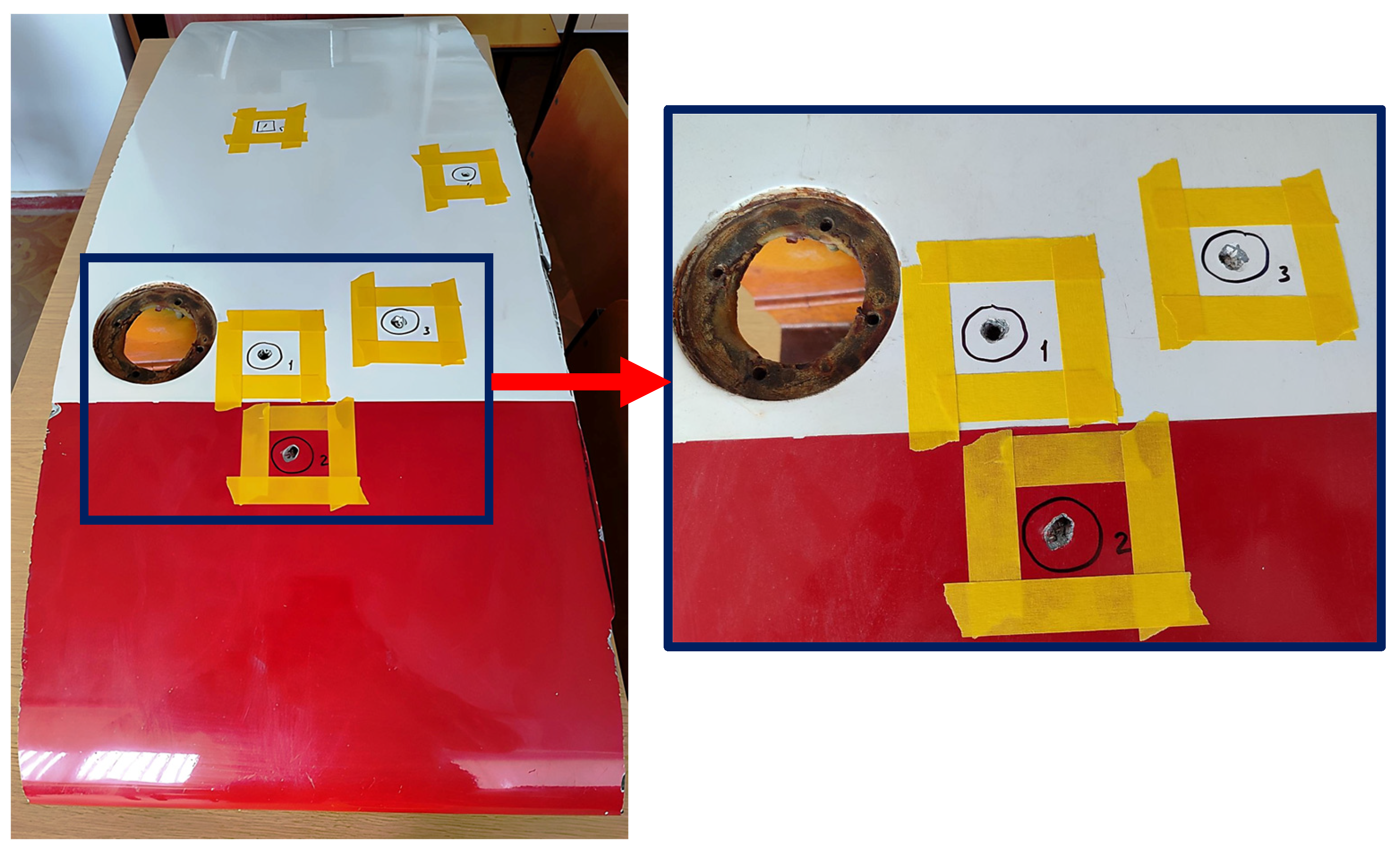Composite patches can be applied not only for composite structure repair but also for the repair of structures made from metals and alloys [14]. For damaged structures (Figure 1), it is possible to select composite patches that possess the most suitable properties required for structural load-carrying ability renovation. If the damaged area can be accessed from both sides, a double-sided lap joint can be used [15]. In addition, several types of adhesives can be used simultaneously to increase the strength of the adhesive joints [16,17,18]. Typically, different adhesives are used for joining damaged structural elements with composite patches. Adhesive joints can be efficiently implemented for joining relatively thin-walled structures. Such joints guarantee load transferring over entire elements of the total structure without local (discrete) fasteners, which, generally, are stress concentrators. Moreover, the adhesive joint allows us to realize such important properties as air-tightness, low weight, manufacturability, and aerodynamic efficiency, that are particularly important for aerospace objects. Besides numerical simulations, experimental investigations of joints [19] and the strength of reinforced plates [20] have also been conducted.

The repair of damaged structures through composite patches is a fairly well-known process. Many studies have been conducted in this field and multiple theories for joint stress state definition have been developed [16,21]. However, as a rule, composite patches are used as non-cured materials for the repair process and require correspondent conditions for composite curing, i.e., temperature, pressure, and time. This requirement makes this approach non-realizable practically in field conditions and demands special workshops with equipment, demounting articles, or units from damaged structures. This leads to relatively high time and financial costs given the repair quality. In the case of using hot-curing prepregs for repair patches, they can be produced partially polymerized. Then, during bonding with hot-curing adhesive, both the final polymerization of composite material of the patch and the curing of adhesive will occur simultaneously, and the patch will take the shape of the surface being repaired. Application of ready patches with required material properties and reduces expenses related to manufacturing and the total repair process. To join a damaged article with a ready patch, one has to apply less pressure than when undertaking the same process for bonding and curing composite patch layers [22]. Here, special vacuum equipment and entire structure heating are not required. Similar repairs can be conducted with minimal equipment and in a short period of time. Analytical solutions addressing the stress state in lap joints have been proposed for various types, including beam-type joints [21] and coaxial tubular joints [23]. A detailed review of existing analytical models is presented in [16,24]. In adhesive joints, the thickness of the adhesive layer is typically several orders of magnitude smaller than the thickness of the parts being joined. Moreover, the elastic properties of the adhesive often differ substantially from the parameters of the structures being joined. These factors, along with the presence of high stress gradients within the adhesive layer, necessitate the use of highly refined finite element meshes, which complicates and slows down numerical simulations—particularly in problems requiring repeated computations, such as optimization tasks. One-dimensional analytical models of the stress state, based on well-established theories of beams, plates, and interlayers, offer a computationally efficient alternative without a significant loss of accuracy, and therefore remain highly relevant in design applications. In addition, such analytical models provide deeper insight into the stress distribution within the joint and facilitate the study of how stress levels in joint elements depend on structural parameters.

To verify the proposed mathematical model, we will compare its results with those obtained via finite element modeling. Calculations based on the one-dimensional model are implemented in Python 3.10, while the finite element simulations are performed using the COMSOL Multiphysics 5.4 software package. The axial symmetry of the problem will allow us to construct a two-dimensional finite element model (in the axial cross-section plane), in which the cross-section of the adhesive and the bonded plates was discretized into triangular elements. All components of the structure are modeled as linearly elastic, three-dimensional axisymmetric solids using COMSOL’s “Solid Mechanics” module. Perfect bonding (without slip) between the adhesive and the adherends is assumed.

2. Mathematical Model and Materials

The surfaces of airframe structures are not flat in most cases. At the same time, they are mainly represented by single curved surfaces. Moreover, the curvature, relative to the size of the repair zone and the patch, can be considered very large and is not taken into account in the optimization study.

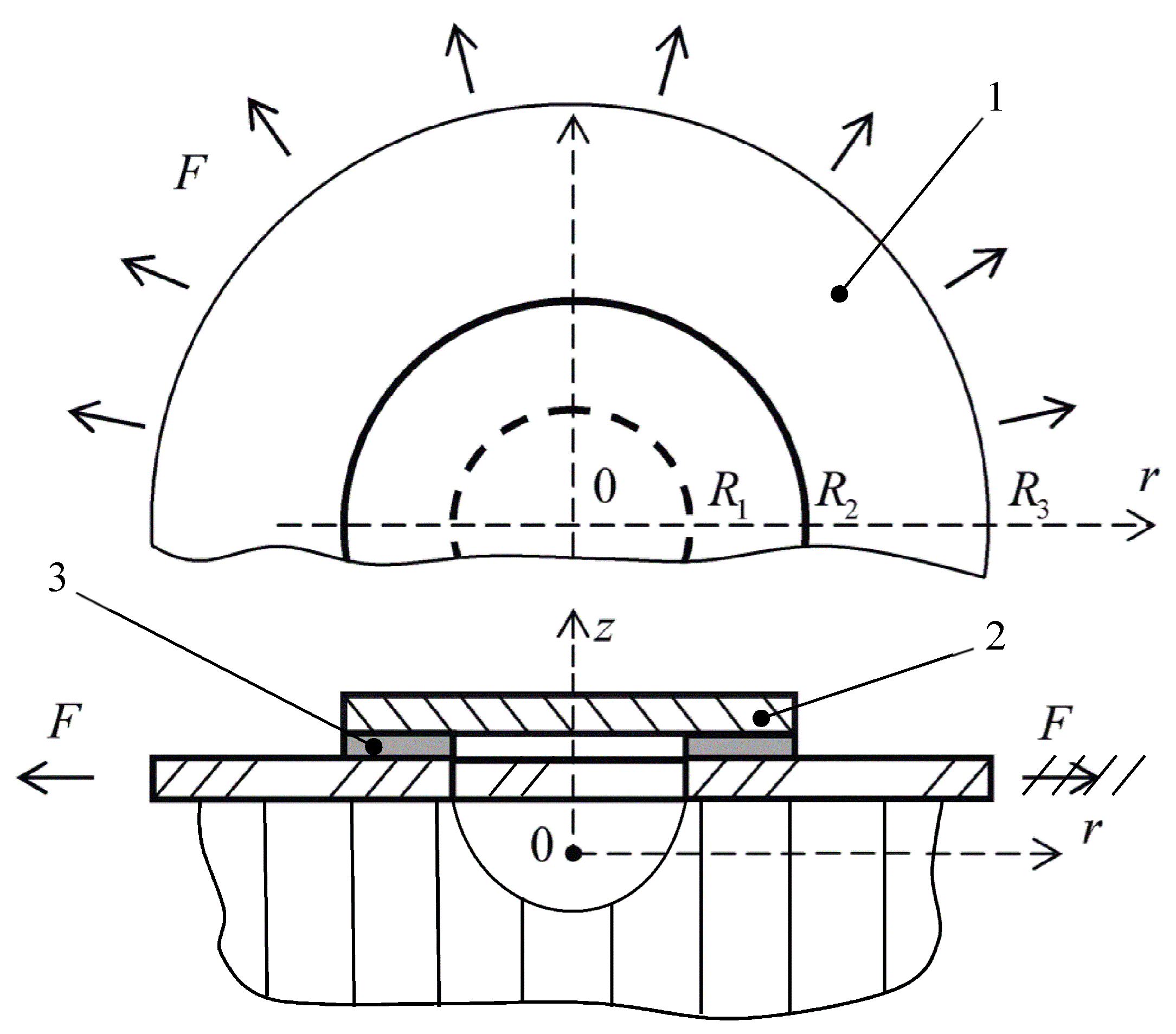
To simulate the problem, the structure shown in Figure 2 is considered. The radius of the hole in the main plate is R₁, and the radius of the patch is R₂. Let us assume that the thickness of the main plate is δ₁ and the thickness of the patch is δ₂. There is an adhesive layer between the plates, and its thickness is δ₀. Suppose the outer radius of the main plate is R₃. It is obvious that if the radius R₃ is large enough, then the influence of the boundary conditions on the outer boundary of the plate and the shape of the outer boundary of the plate will not affect the stress state of the joint. Let the main plate be loaded with tensile forces F applied along the radius R₃.

The main plate is on a core material (honeycomb or foam plastic), which is sufficiently rigid and limits the bending of the main plate; therefore, the transverse displacements of the main plate can be considered equal to zero. There is no core material under the hole in the main plate. This model corresponds to either a through hole or a blind hole formed during repair. This repair technique is well-known and widely used in the repair process of aircraft equipment, during which a hole of arbitrary shape is drilled into a round one to reduce stress concentration [25].

The structure (Figure 2) is divided into multiple sub-regions: the adhesive region and two regions outside the adhesive, the patch above the hole and the main plate surrounding the adhesive joint.

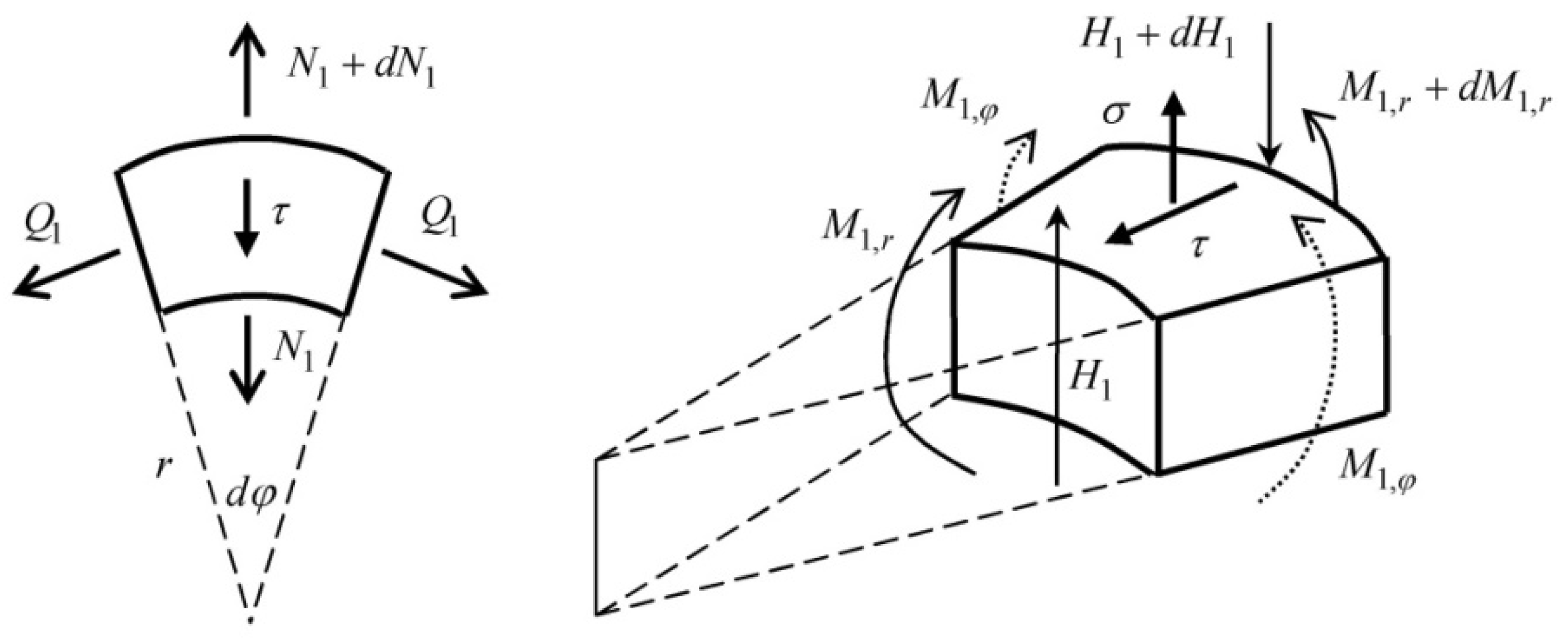
First of all, let us consider the adhesive region $r\in \left[R_1;\hspace{0.33em}{R}_2\right]$. The equilibrium of the differential element of the lower plate is shown in Figure 3.

The subscript “1” refers to the main plate and the subscript “2” refers to the circular patch located within the adhesive region. The equilibrium equations of the differential elements of the patch and the main plate are as follows:

$${\displaystyle \frac{N_1-Q_1}{r}}+{\displaystyle \frac{d{N}_1}{dr}}-\tau =0, {\displaystyle \frac{N_2-Q_2}{r}}+{\displaystyle \frac{d{N}_2}{dr}}+\tau =0,$$

(1)

$${\displaystyle \frac{M_{2,r}-M_{2,\phi }}{r}}+{\displaystyle \frac{d{M}_{2,r}}{dr}}-H_2+{\displaystyle \frac{{\delta }_2}{2}}\tau =0, {\displaystyle \frac{H_2}{r}}+{\displaystyle \frac{d{H}_2}{dr}}+\sigma =0,$$

(2)

where $Q_k$, $N_k$—normal forces on plate $k$ in circumferential and radial directions, $k \mathrm{i}\mathrm{s} \mathrm{e}\mathrm{q}\mathrm{u}\mathrm{a}\mathrm{l} \mathrm{t}\mathrm{o} 1,\hspace{0.33em}2$; $\tau$, $\sigma$—shear and normal (tear-off) stresses in the adhesive layer; $M_{k,r}$—bending moment in layer $k$ in the radial direction; $M_{k,\phi }$—bending moment in layer $k$ in the circumferential direction; $H_k$—shear force in layer $k$.

The shear and normal stresses in the adhesive layer are constant through the thickness of the adhesive and are proportional to the difference in the longitudinal; accordingly, transverse displacements of the sides of the plates facing the adhesive layer [25]

$$\tau =P_1\left(u_1-u_2-{\displaystyle \frac{{\delta }_2}{2}}{\displaystyle \frac{d{w}_2}{dr}}\right), \sigma =P_2\cdot w_2,$$

(3)

where $P_1$ and $P_2$ are the rigidity of the adhesive layer in shear and tear-off, respectively, $P_1=G_0/{\delta }_0$, $P_2=\left(E_0/{\delta }_0\right){\left(1-{\mu }_0^2\right)}^{-1}$, where, respectively, $E_0$, $G_0$, ${\mu }_0$ are the modulus of elasticity, shear modulus, and Poisson’s ratio of the adhesive; $w_2$ is the transverse displacements of the patch (the transverse displacements of the main plate are zero since it lies on a rigid base); and $u_k$ is the longitudinal (radial) displacements of layers, where k is equal to 1, 2.

Hooke’s law for plates is written as

$$N_k=B_k\left({\epsilon }_{k,r}+{\mu }_k{\epsilon }_{k,\phi }\right), Q_k=B_k\left({\epsilon }_{k,\phi }+{\mu }_k{\epsilon }_{k,r}\right),$$

(4)

where $B_k={\delta }_k{E}_k{\left(1-{\mu }_k^2\right)}^{-1}$—membrane stiffness of plates; ${\mu }_k$—Poisson’s ratio of the plate material $k$, $k=1,\hspace{0.33em}2$; $E_k$—modulus of elasticity of the plate material $k$; ${\epsilon }_{k,\phi }$ and ${\epsilon }_{k,r}$—deformation of layer $k$ in circumferential and radial directions.

Radial displacements are related to deformation through specific relationships:

$${\epsilon }_{k,r}={\displaystyle \frac{d{u}_k}{dr}}, {\epsilon }_{k,\phi }={\displaystyle \frac{u_k}{r}}.$$

(5)

Bending moments in the patch are represented as follows (by the Kirchhoff–Love theory):

$$M_{2,r}=D_2\left({\displaystyle \frac{d^2{w}_2}{d{r}^2}}+{\displaystyle \frac{{\mu }_2}{r}}{\displaystyle \frac{d{w}_2}{dr}}\right), M_{2,\phi }=D_2\left({\mu }_2{\displaystyle \frac{d^2{w}_2}{d{r}^2}}+{\displaystyle \frac{1}{r}}{\displaystyle \frac{d{w}_2}{dr}}\right),$$

(6)

where $D_2={\displaystyle \frac{E_2{\delta }_2^3}{12\left(1-{\mu }_2^2\right)}}$ is the bending stiffness of the patch.

Outside the adhesive region, in Section 3 and Section 4 (Figure 3), the stress state of the patch and the main plate is characterized by the well-known equations of axisymmetric deformation of circular plates [25].

3. Statement of the Problem

3.1. The Adhesive Region

Differentiating (4) and using (1)–(3) and relations (5)–(7), we can obtain a system of equations for the stresses in the adhesive layer:

$${\displaystyle \frac{d^3\tau }{d{r}^3}}+{\displaystyle \frac{2}{r}}{\displaystyle \frac{d^2\tau }{d{r}^2}}-\left(a_1+{\displaystyle \frac{1}{r^2}}\right){\displaystyle \frac{d\tau }{dr}}+\left({\displaystyle \frac{1}{r^3}}-{\displaystyle \frac{a_1}{r}}\right)\tau +P{a}_2\sigma =0;$$

(7)

$${\displaystyle \frac{d^4\sigma }{d{r}^4}}+{\displaystyle \frac{2}{r}}{\displaystyle \frac{d^3\sigma }{d{r}^3}}-{\displaystyle \frac{1}{r^2}}{\displaystyle \frac{d^2\sigma }{d{r}^2}}+{\displaystyle \frac{1}{r^3}}{\displaystyle \frac{d\sigma }{dr}}+a_3\sigma -K{a}_2\left({\displaystyle \frac{\tau }{r}}+{\displaystyle \frac{d\tau }{dr}}\right)=0;$$

(8)

where $a_1=P_1\left({\displaystyle \frac{1}{B_1}}+{\displaystyle \frac{1}{B_2}}+{\displaystyle \frac{{\delta }_2^2}{4D_2}}\right)$, $a_2=-{\displaystyle \frac{{\delta }_2}{2D_2}}$, $a_3={\displaystyle \frac{P_2}{D_2}}$.

If we express σ from (7) and substitute into (8), we obtain the differential equation

$$\begin{gathered} {\displaystyle \frac{d^7\tau }{d{r}^7}}+{\displaystyle \frac{4}{r}}{\displaystyle \frac{d^6\tau }{d{r}^6}}-\left(a_1+{\displaystyle \frac{6}{r^2}}\right){\displaystyle \frac{d^5\tau }{d{r}^5}}+\left({\displaystyle \frac{18}{r^3}}-{\displaystyle \frac{3a_1}{r}}\right){\displaystyle \frac{d^4\tau }{d{r}^4}}+\left({\displaystyle \frac{3a_1}{r^2}}-{\displaystyle \frac{51}{r^4}}+a_3\right){\displaystyle \frac{d^3\tau }{d{r}^3}}+ \\ \left({\displaystyle \frac{126}{r^5}}-{\displaystyle \frac{6a_1}{r^3}}+{\displaystyle \frac{2a_3}{r}}\right){\displaystyle \frac{d^2\tau }{d{r}^2}}+\left({\displaystyle \frac{9a_1}{r^4}}-{\displaystyle \frac{225}{r^6}}-{\displaystyle \frac{a_3}{r^2}}+a_2^2{P}_1{P}_2-a_1{a}_3\right){\displaystyle \frac{d\tau }{dr}}+ \\ \left({\displaystyle \frac{225}{r^7}}-{\displaystyle \frac{9a_1}{r^5}}+{\displaystyle \frac{a_3}{r^3}}+{\displaystyle \frac{a_2^2{P}_1{P}_2-a_1{a}_3}{r}}\right)\tau =0. \end{gathered}$$

(9)

We will seek the general solution of Equation (9) in the following form:

$$\tau ={\sum }_{n=1}^6{C}_n{K}_1\left({\lambda }_{n}r\right)+{\displaystyle \frac{C_7}{r}};$$

(10)

where $K_1\left({\lambda }_{n}r\right)$—modified Bessel functions of the second kind (Macdonald functions); $C_n$—arbitrary constants.

After substituting (9) into (8), we obtain the characteristic equation.

${\lambda }^6-a_1{\lambda }^4+a_3{\lambda }^2+a_2^2{P}_1{P}_2-a_1{a}_3=0$; the roots of this equation are the coefficients ${\lambda }_n$, $n=1,\dots ,6$, included in (10).

From (7), we can easily find the normal (tear-off) stresses in the adhesive layer:

$$\sigma ={\sum }_{n=1}^6{C}_n{\alpha }_n{K}_0\left({\lambda }_{n}r\right),$$

(11)

where ${\alpha }_n=\left({\lambda }_n^3-a_1{\lambda }_n\right){\left(P_1{a}_2\right)}^{-1}$.

It is important to mention that the stress state of rods or beams that are overlapped by an elastic connecting layer [25] is expressed through linear combinations of exponential functions. In this case, because of the circular symmetry, the counterparts of the exponential functions are unbounded and non-periodic modified Bessel functions.

From (1), using (4) and (5), we obtain

$${\displaystyle \frac{d^2{u}_1}{d{r}^2}}+{\displaystyle \frac{1}{r}}{\displaystyle \frac{d{u}_1}{dr}}-{\displaystyle \frac{u_1}{r^2}}-{\displaystyle \frac{\tau }{B_1}}=0, {\displaystyle \frac{d^2{u}_2}{d{r}^2}}+{\displaystyle \frac{1}{r}}{\displaystyle \frac{d{u}_2}{dr}}-{\displaystyle \frac{u_2}{r^2}}+{\displaystyle \frac{\tau }{B_2}}=0$$

The solution to these equations is as follows:

$$\begin{gathered} u_1={\displaystyle \frac{1}{B_1}}\sum _{n=1}^6{\displaystyle \frac{C_n}{{\lambda }_n^2}}{K}_1\left({\lambda }_{n}r\right)+{\displaystyle \frac{C_7}{4B_1}}r\left(2\mathit{ln}r-1\right)+C_{8}r+{\displaystyle \frac{C_9}{r}} \\ {u}_2={\displaystyle \frac{1}{B_2}}\sum _{n=1}^6{\displaystyle \frac{C_n}{{\lambda }_n^2}}{K}_1\left({\lambda }_{n}r\right)-{\displaystyle \frac{C_7}{4B_2}}r\left(2\mathit{ln}r-1\right)+C_{10}r+{\displaystyle \frac{C_{11}}{r}} \end{gathered}$$

From Equation (3), it is straightforward to determine the transverse displacements of the patch w₂. Using the relations for stresses in the adhesive layer (10) and (11), longitudinal and transverse displacements of the patch and the main plate, it will be easy from (4)–(6) to find the radial and circumferential forces in the plates and the bending moments in the patch. The shear forces H₂ in the patch are found in (2).

3.2. The Regions Outside the Adhesive

There are two regions outside the adhesive region. One of them is the main plate ($R_2\le r\le R_3$), and the other is the patch above the cutout ($0\le r\le R_1$). The index “4” denotes the displacements and force factors in the main plate outside the adhesive region. The index “3” denotes the displacements and force factors in the patch above the cutout. The displacements in these regions are described by the known equations of deformation of round plates in the absence of shear forces [23]:

$${\displaystyle \frac{d^2{u}_m}{d{r}^2}}+{\displaystyle \frac{1}{r}}{\displaystyle \frac{d{u}_m}{dr}}-{\displaystyle \frac{u_m}{r^2}}=0, {\displaystyle \frac{d^3{w}_3}{d{r}^3}}+{\displaystyle \frac{1}{r}}{\displaystyle \frac{d^2{w}_3}{d{r}^2}}-{\displaystyle \frac{1}{r^2}}{\displaystyle \frac{d{w}_3}{dr}}=0,$$

where $m=3,\hspace{0.33em}4$.

The solutions to these equations are as follows:

$$U_3=c_{1}r+{\displaystyle \frac{c_2}{r}}, U_4=c_{3}r+{\displaystyle \frac{c_4}{r}}, W_3=s_1+s_2\mathit{ln}r+s_3{r}^2.$$

Bending moments and radial and circumferential forces are found using (4)–(6).

3.3. Boundary Conditions

The unknown coefficients are established based on the boundary conditions and the conjugation conditions at the edges of the regions.

At point r = 0, the transverse displacements must be limited in magnitude, and the radial displacements are zero. It follows from this that $c_2=0$ and $s_2=0$.

On the outer boundary of the main plate, tensile radial forces are specified in the form

$$N_4\left(R_3\right)=F.$$

At the boundaries of the adhesive region, we have the following conditions:

$$\begin{gathered} N_4\left(R_2\right)=N_1\left(R_2\right), U_4\left(R_2\right)=U_1\left(R_2\right), N_2\left(R_2\right)=M_{2,r}\left(R_2\right)=N_2\left(R_2\right)=0, \\ {N}_1\left(R_1\right)=0, U_2\left(R_1\right)=U_3\left(R_1\right), W_2\left(R_1\right)=W_3\left(R_1\right), {\left.{\displaystyle \frac{d{W}_2}{dr}}\right|}_{r=R_1}={\left.{\displaystyle \frac{d{W}_3}{dr}}\right|}_{r=R_1}, \\ {M}_{2,r}\left(R_1\right)=M_{3,r}\left(R_1\right), N_2\left(R_1\right)=N_3\left(R_1\right), H_2\left(R_1\right)=H_3\left(R_1\right). \end{gathered}$$

In addition, the radial displacements $U_1\left(r\right)$ and $U_2\left(r\right),$ and the transverse displacements of the patch $W_2\left(r\right)$, must turn Equation (3) into an identity. From this, it follows that

$$C_7=0, -C_9+C_{11}+{\displaystyle \frac{C_7}{P_1}}=0, C_{10}-C_8=0.$$

(12)

Thus, we obtain a closed system of linear equations with respect to unknown coefficients.

4. Numerical Simulation of the Problem

To analyze the stress state of the adhesive joint and validate the suggested analytical model, we will consider the bonding of two aluminum ($E^{\left(1\right)}=E^{\left(2\right)}=70$ GPa, $\mu =0.28$ Poisson’s ratio) plates. The thickness of the plates is ${\delta }_1={\delta }_2=1$ mm. These plates are adhered using an adhesive with elastic properties of $G_0=0.3125$ GPa, $E_0=0.8$ GPa, and a thickness of ${\delta }_0=0.1$ mm. The radius of the hole in the plate is $R_1=20$ mm, while the radius of the patches is $R_2=50$ mm. In the calculations, we will assume that the main plate has an infinitely large radius $R_3=\infty$ mm. This assumption is justified by the fact that the influence of the hole and patches on the stress–strain state of the main plate is localized. This holds true for a relatively large plate of any shape with a significant distance of the cutout from its edge, we can assume that the main plate is infinitely large. Along the outer boundary of the main plate, tensile radial forces $F$ are specified. Obviously, in this scenario, the radial forces in the main plate at infinity are also equal to $F$.

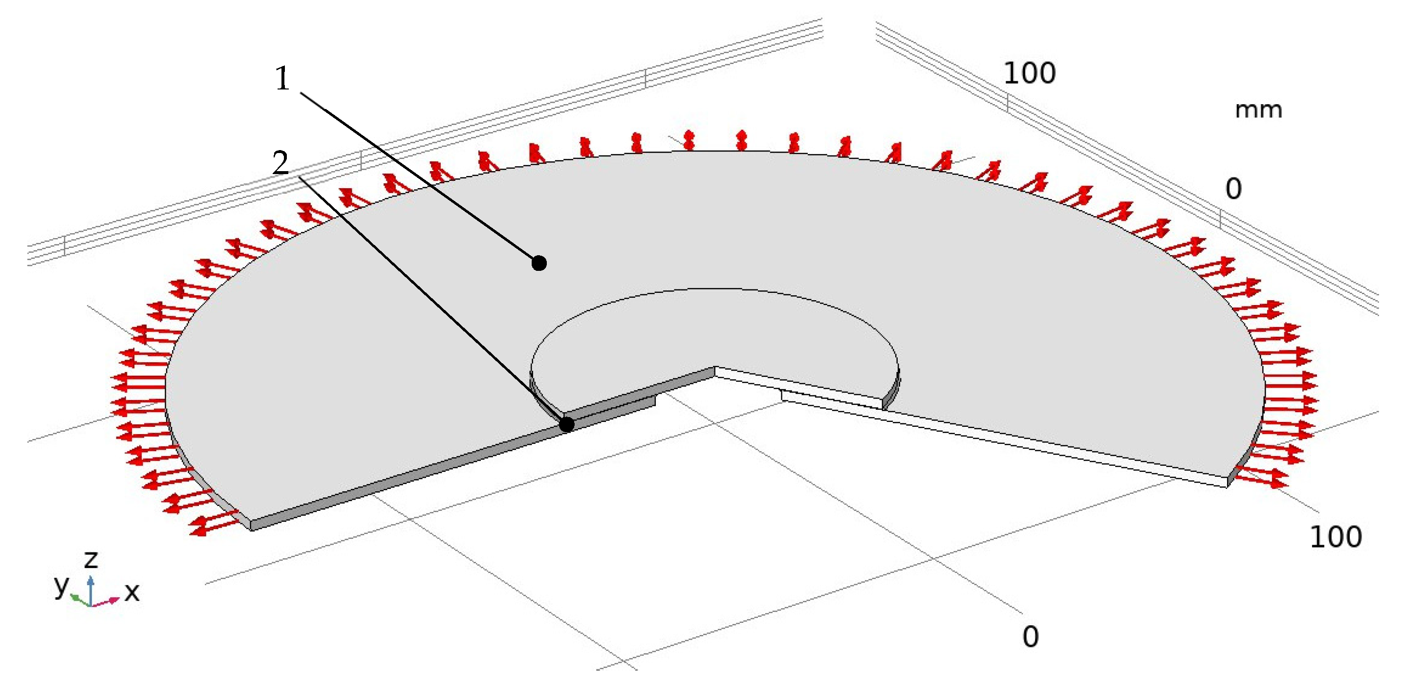
To validate the proposed analytical model of the stress–strain state of the adhesive joint, an axisymmetric finite element model was developed. The geometric shape of the structure is illustrated in Figure 4. The outer radius is $R_3=3R_2$. Radial normal stress $\sigma ={\displaystyle \frac{F}{{\delta }_1}}$ is applied to the external edge of the plate. The bottom surface of the plate is fixed with a “roller” support, while the remaining surfaces are free of stresses.

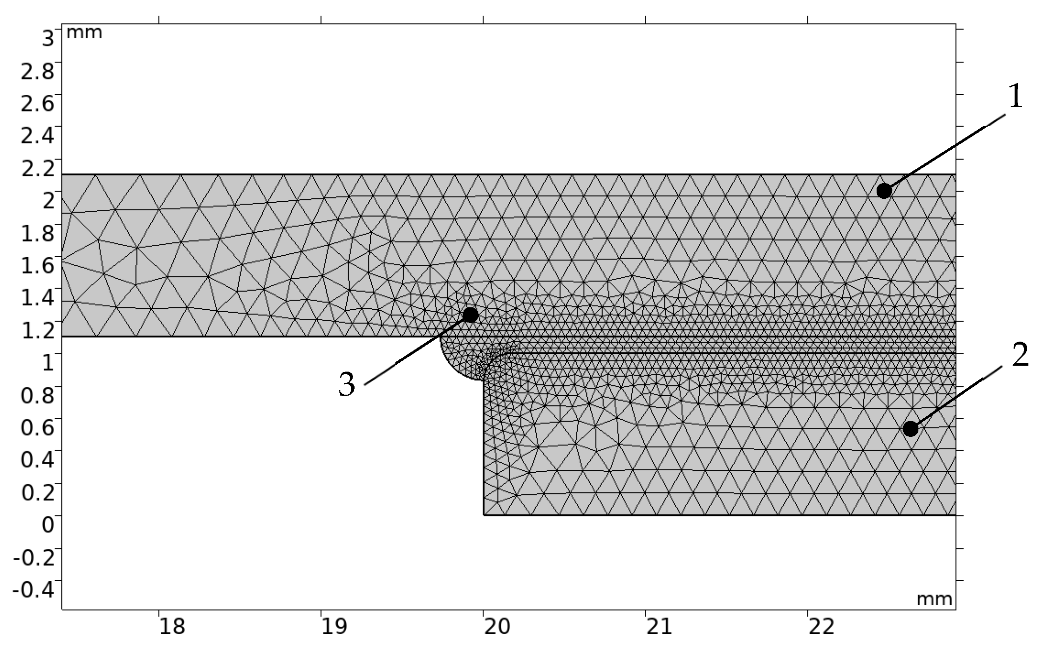
The finite element model of the adhesive joint includes chamfers and excess squeezed-out adhesive (Figure 5), which shows a fragment of the model in the vicinity of the edge of the adhesive seam. Since the highest stress gradients occur within the adhesive layer, it was meshed with the smallest element size. In the mesh shown (Figure 5), the element size in the adhesive layer ranges from 0.25 δ₀ to 0.5 δ₀ units, while the maximum element size in the outer region of the plate is equal to half the plate thickness. The mesh consisted of 32,321 elements with a minimum quality of 0.5382 and an average quality of 0.8831.

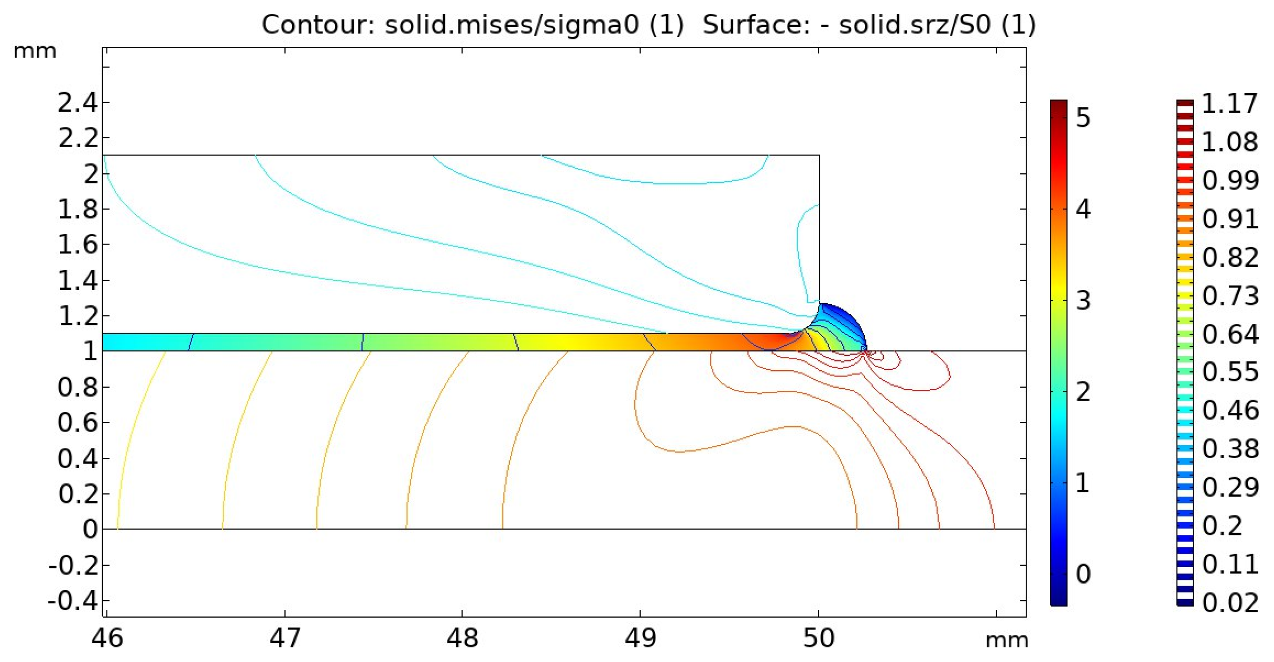
The stress distribution in the structure by the FEM is shown in Figure 6.

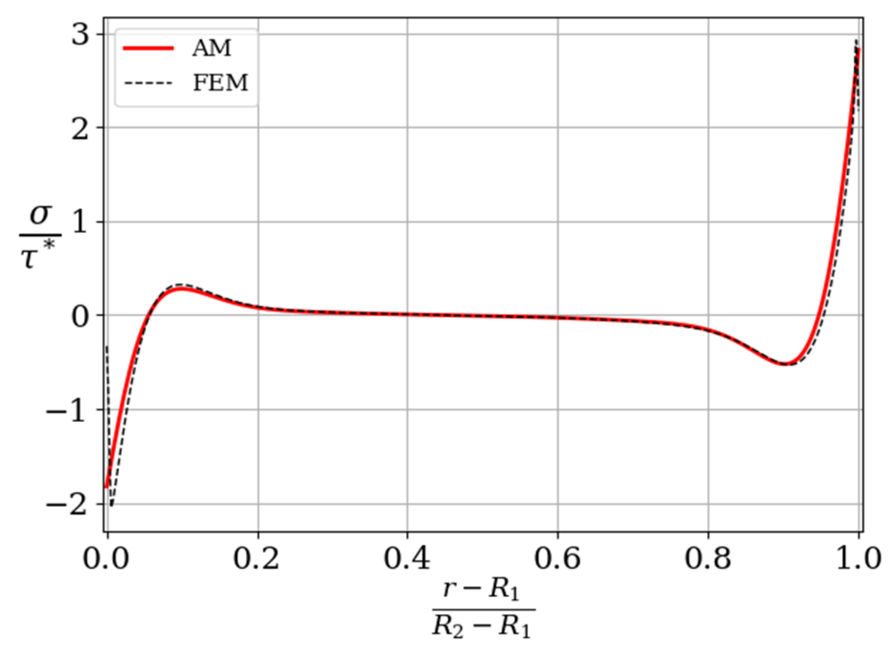
The shear stresses in the adhesive layer τ are shown in Figure 7.

The stresses calculated using the analytical model (AM) proposed in the paper are shown by a solid line. The shear stresses in the median plane of the adhesive joint calculated using the finite element model (FEM) are shown by a dotted line. The stresses are shown in dimensionless form, as the ratio of the acting stresses to some stresses is ${\tau }^{*}={\displaystyle \frac{F}{R_2-R_1}}$. Here, F is the linear forces applied to the end of the main plate, R₂ − R₁ is the width of the adhesive seam.

As can be seen, the stress distributions in the adhesive layer near the edge of the joint, obtained using the proposed mathematical model and finite element modeling, differ significantly. This phenomenon is well known and results from the assumption in classical adhesive stress models that the stresses are uniformly distributed through the adhesive thickness. In such models, the shear stresses reach their maximum exactly at the edge of the adhesive joint, which contradicts the shear stress reciprocity law requiring that stresses vanish at the free edge. This known inconsistency has motivated the development of more sophisticated mathematical models for adhesive joints, for example [21]. Existing studies show that in reality, the shear stress maximum is located slightly inward—at a distance approximately equal to the adhesive layer thickness from the edge. Nevertheless, the peak stress values, which are critical for strength analysis, are very close to those obtained by analytical models.

Normal stresses in the adhesive layer σ are shown in Figure 8.

As in the previous graph, the solid line shows the stresses calculated using the analytical model (AM) proposed in the work. The dotted line shows the shear stresses in the median plane of the adhesive joint, calculated using the finite element model (FEM).

5. Results and Discussion

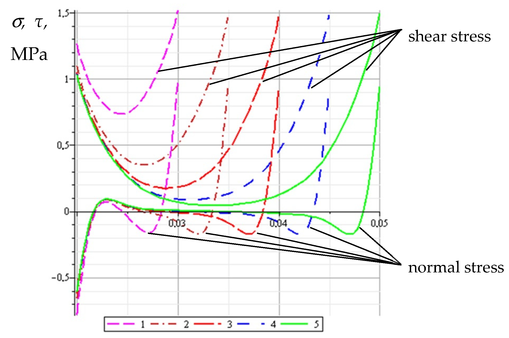
The distribution of normal (lower curves) and shear stresses (upper curves) in the adhesive region depending on the radius of the repair patch are shown in Figure 9. Five cases of the patch radius are considered; curve 1 corresponds to the radius of the patch R₂ = 30 mm, curve 2 is R₂ = 35 mm, curve 3 is R₂ = 40 mm, curve 4 is R₂ = 45 mm, and curve 5 is R₂ = 50 mm. The thickness of the main plate for all cases δ₁ is equal to 1 mm, the thickness of the patch δ₂ is equal to 1 mm, the hole’s radius R₁ is equal to 20 mm, and the thickness of the adhesive layer δ₀ is equal to 0.1 mm.

The graphs of normal and shear stresses in Figure 9 depict the stress state in the adhesive region and clearly demonstrate the characteristic feature of load transfer in a single lap joint—with an increase in the joint area, the degree of uneven stress distribution increases significantly, practically excluding the central part of the joint from the load transfer process [26,27]. For a more effective study of the stress distribution in the adhesive zone, as well as for a quantitative assessment of the unevenness of their distribution, dimensionless graphs were used for further analysis.

The dependencies of the distribution of normal (lower curves) and shear stresses (upper curves) in the adhesive region on the thickness of the repair patch are shown in Figure 10. Three cases of patch thickness are considered. The thickness of the main plate for all cases δ₁ is equal to 1 mm, the hole’s radius R₁ is equal to 20 mm, and the thickness of the adhesive layer δ₀ is equal to 0.1 mm. In each graph, curve 1 corresponds to the radius of the patch R₂ = 30 mm, curve 2 is R₂ = 35 mm, curve 3 is R₂ = 40 mm, curve 4 is R₂ = 45 mm, and curve 5 is R₂ = 50 mm. The stress is shown in a dimensionless form, as a ratio of the effective stresses to some stresses ${\tau }^{*}={\displaystyle \frac{F}{R_2-R_1}}$. Here, F is the linear force applied to the end of the main plate and $R_2-R_1$ is the width of the adhesive seam.

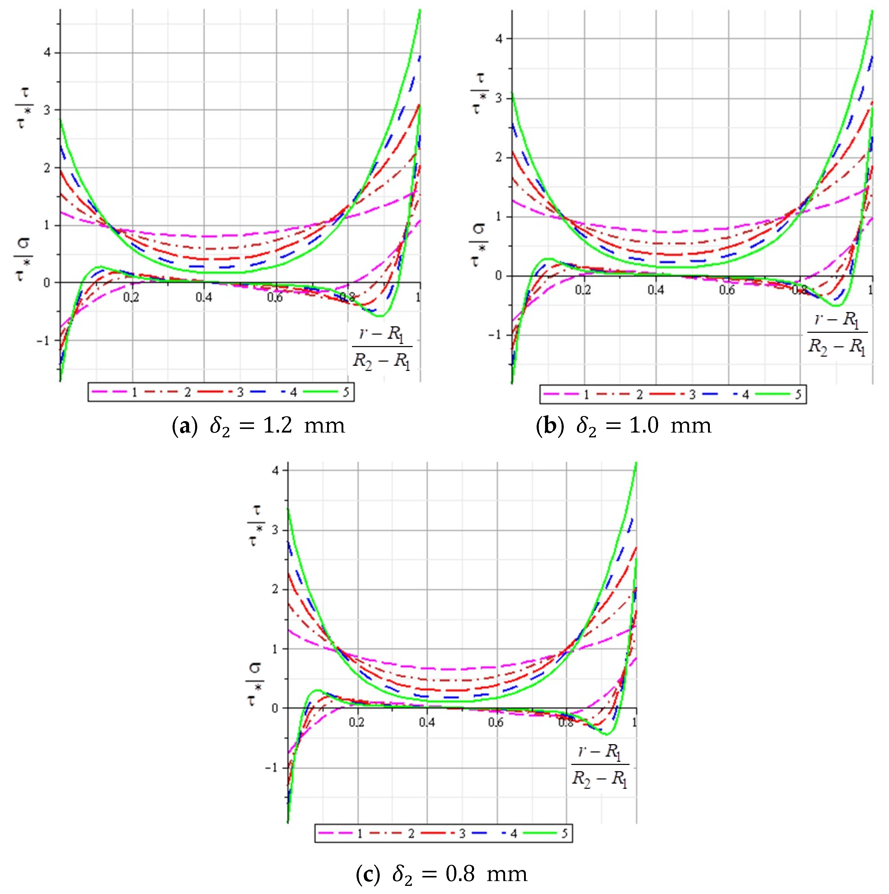
The dependencies of the distribution of normal (lower curves) and shear stresses (upper curves) in the adhesive region on the area of adhesive (radius of the repair patch) are shown in Figure 11. Three cases of the radius of the patch are considered. The thickness of the main plate for all cases δ₁ is equal to 1 mm, the thickness of the adhesive layer δ₀ is equal to 0.1 mm. In each graph, curve 1 corresponds to the thickness of the patch δ₂ = 0.8 mm, curve 2 is δ₂ = 1.0 mm and curve 3 is δ₂ = 1.2 mm. The stress, as in the previous graphs, is shown in dimensionless form.

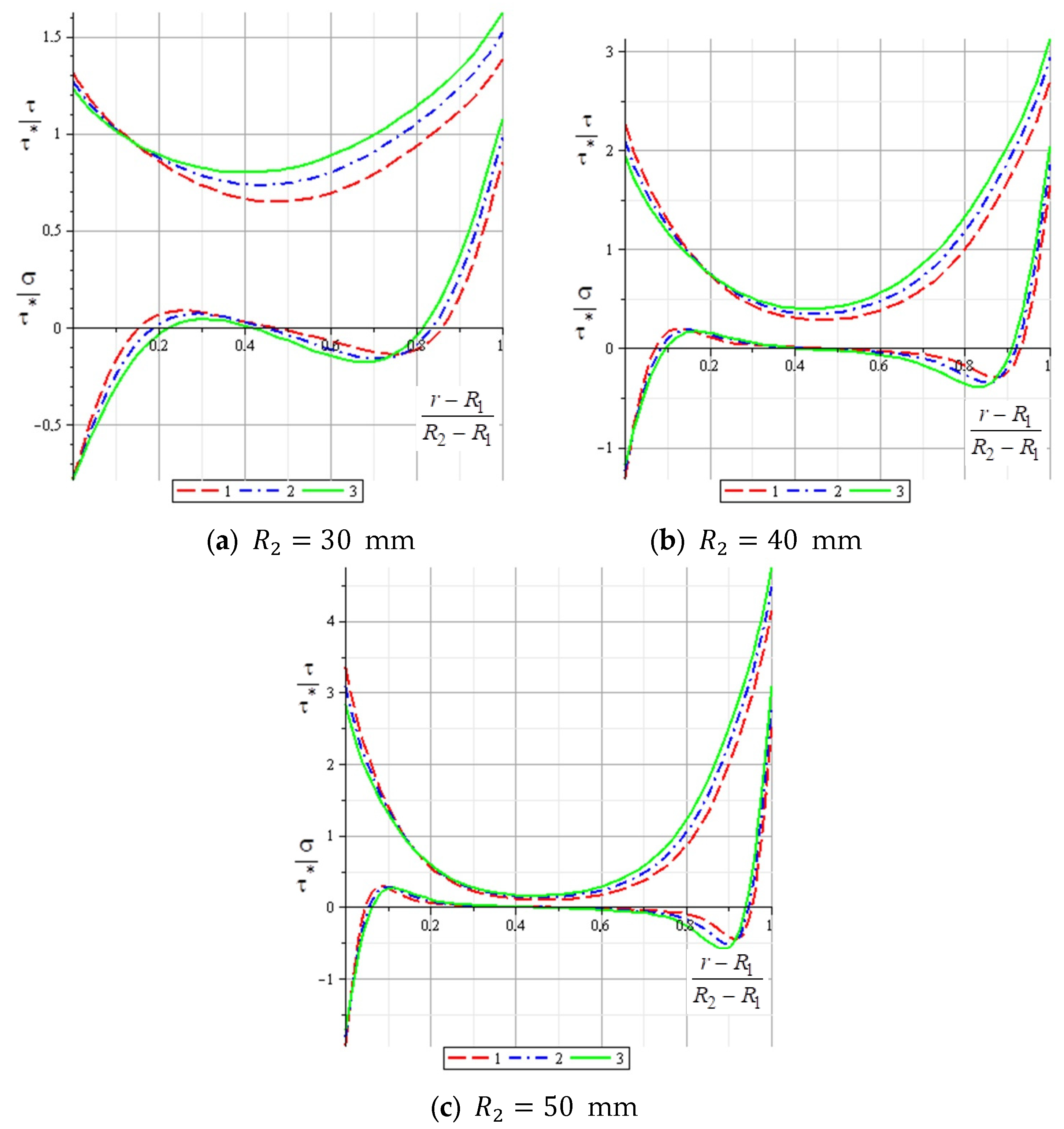
The dependencies of the distribution of normal (lower curves) and shear stresses (upper curves) in the adhesive region on the adhesive layer thickness are shown in Figure 12. Three cases of the adhesive layer are considered. The thickness of the main plate for all cases δ₁ is equal to 1 mm, the thickness of the patch δ₂ is equal to 1 mm. In each graph, curve 1 corresponds to the thickness of the adhesive layer δ₀ = 0.08 mm, curve 2 is δ₀ = 0.1 mm, and curve 3 is δ₂ = 0.12 mm. The stress, as in the previous graphs, is shown in dimensionless form.

The nature of the stresses does not depend on the thickness of the patch or the thickness of the adhesive layer but depends on the radius of the patch, that is, on the area of the adhesive area, as can be seen from Figure 10, Figure 11 and Figure 12.

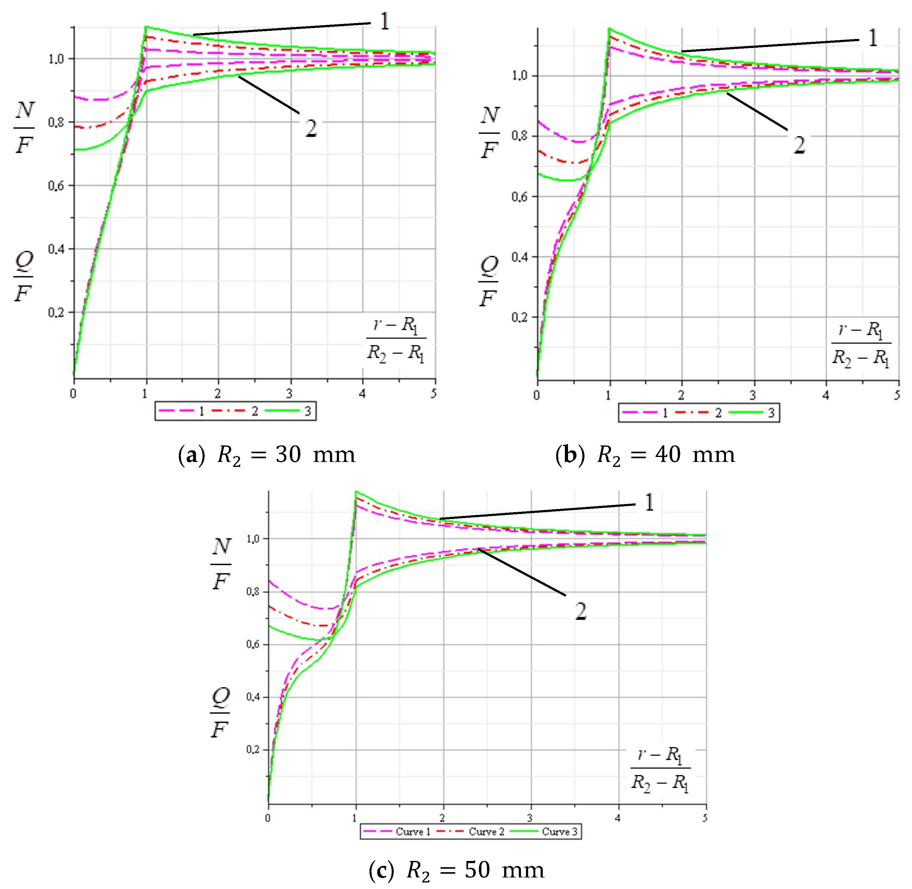
Figure 13 shows the distribution of normal stresses in the main plate in the vicinity of the hole depending on the thickness of the repair patch (curve 1 is radial stress, curve 2 is circular stress). Three cases of patch thickness are considered. The thickness of the main plate for all cases δ₁ is equal to 1 mm, the thickness of the adhesive layer δ₀ is equal to 0.1 mm. In each graph, curve 1 corresponds to the radius of the patch R₂ = 30 mm, curve 2 is R₂ = 40 mm, and curve 3 is R₂ = 50 mm. The stress, as in the previous graphs, is shown in dimensionless form.

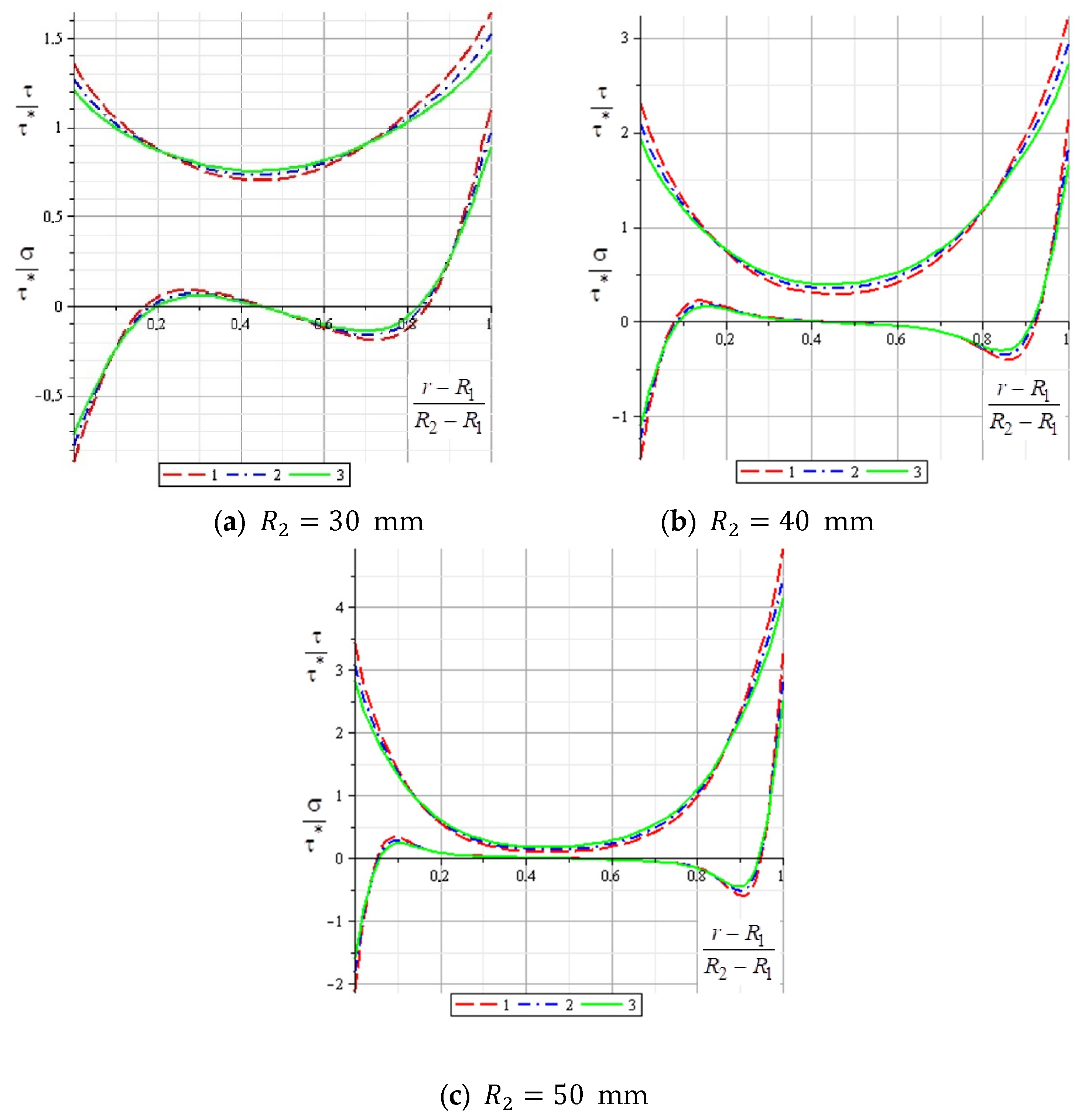
Figure 14 shows the distribution of normal stresses in the main plate in the vicinity of the hole depending on the radius of the repair patch (the ratio of radial stresses to force F is curve 1, the ratio of circular stresses to force F is curve 2). Three cases of the patch’s radius are considered. The thickness of the main plate for all cases is equal to 1 mm, the thickness of the adhesive layer δ₀ is equal to 0.1 mm. In each graph, curve 1 corresponds to the thickness of the patch δ₂ = 0.8 mm, curve 2 is δ₂ = 1.0 mm and curve 3 is δ₂ = 1.2 mm. The stress, as in the previous graphs, is shown in dimensionless form.

The break in the graphs Figure 13 and Figure 14 corresponds to the patch’s limit. Without the patch on the edge of the hole, the normal forces would be zero, and the shear forces would be 2F. In the presence of the patch, we only have an increase in radial forces of less than 20%. That is, as expected, the overlay significantly relieves the hole.

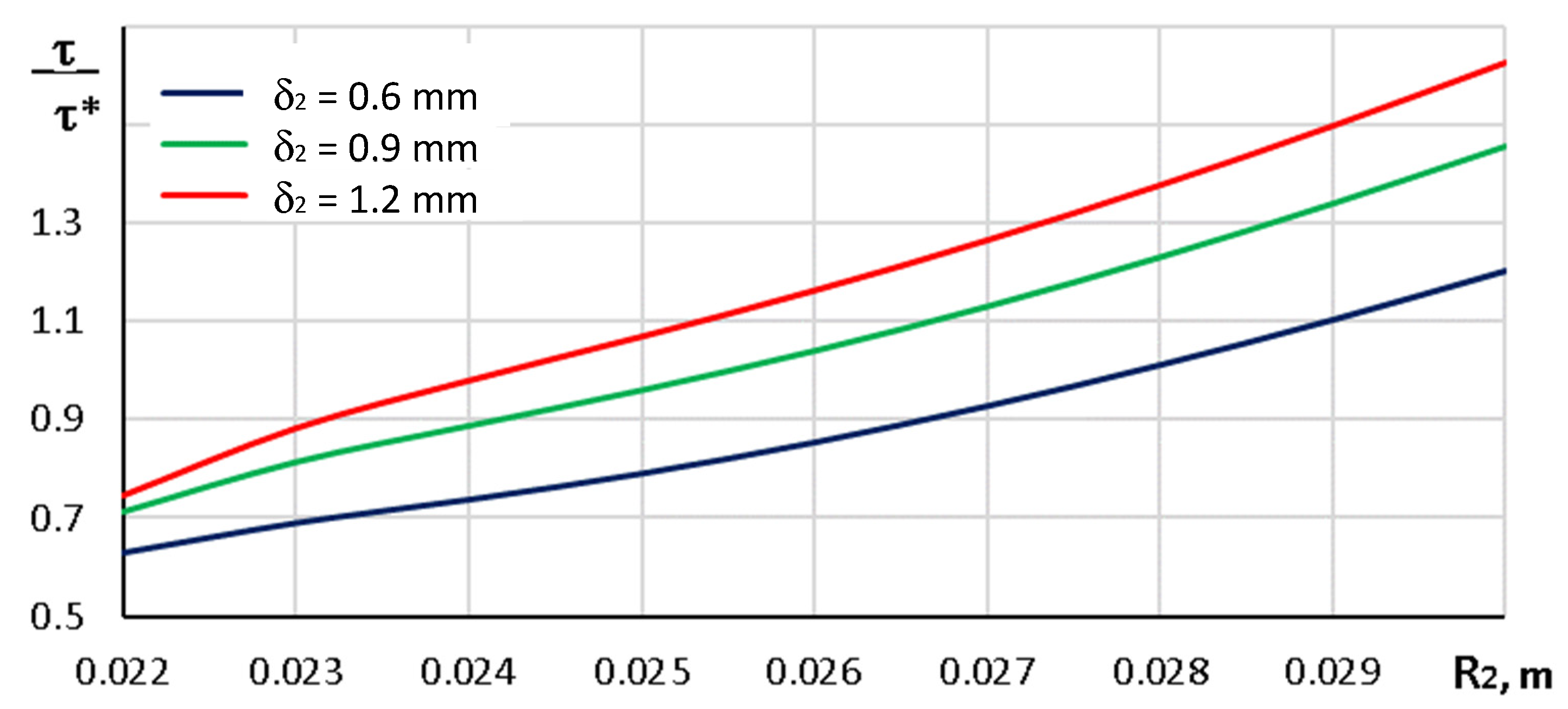
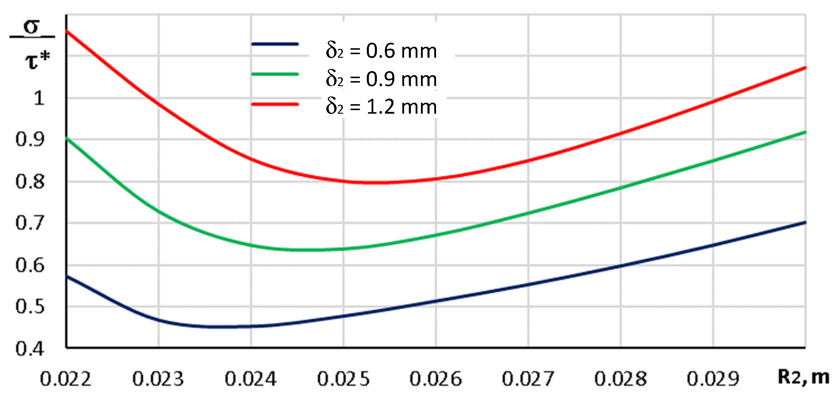
An analysis of the obtained results reveals that the highest loads occur at the end of the patch. The dependence of both normal and shear stresses on the geometric parameters of the patch at this location is presented in Figure 15 and Figure 16, respectively.

The main objective in designing the patch is to reduce stress concentrations in the vicinity of the structural discontinuity (e.g., a hole) by transferring part of the mechanical load from the primary structure to the patch. The optimization criterion for this study is the mass of the patch, expressed as ${\delta }_2{R}_2^2\to min$. The constraints include reducing the circumferential stresses at the hole to a predefined acceptable level $Q_1\left(R_1\right)\le Q^{*}$ and ensuring that the adhesive layer maintains its load-bearing capacity, for example $\sqrt{{\sigma }^2+4{\tau }^2}\le {\sigma }_{max}$.

It is necessary to determine the values of the patch parameters δ₂ and R₂ that satisfy the strength conditions of the structure while minimizing the patch mass. To achieve this goal, any optimization algorithms that involve solving a series of direct problems for different values of δ₂ and R₂ can be used, such as genetic or swarm algorithms. In this case, a brute-force method was applied; the values of the patch radius and its thickness were set (see

Table 1. Results of optimization study.

Patch thickness, δ2, mm		Patch radius, R2, mm
		22.0	23.0	24.0	25.0	26.0	27.0	28.0	29.0	30.0
0.4	I	193.6	211.6	230.4	250.0	270.4	291.6	313.6	336.4	360.0
	II	1.107	0.771	0.608	0.517	0.464	0.432	0.414	0.403	0.398
	III	1.316	1.271	1.247	1.230	1.219	1.209	1.202	1.196	1.191
0.5	I	242.0	264.5	288.0	312.5	338.0	364.5	392.0	420.5	450.0
	II	1.258	0.881	0.698	0.596	0.536	0.498	0.476	0.462	0.454
	III	1.245	1.188	1.157	1.137	1.123	1.112	1.103	1.096	1.091
0.6	I	290.4	317.4	345.6	375.0	405.6	437.4	470.4	504.6	540.0
	II	1.387	0.974	0.773	0.662	0.595	0.554	0.528	0.512	0.502
	III	1.191	1.121	1.084	1.061	1.044	1.032	1.022	1.014	1.008
0.7	I	338.8	370.3	403.2	437.5	473.2	510.3	548.8	588.7	630.0
	II	1.499	1.054	0.838	0.718	0.646	0.601	0.573	0.555	0.543
	III	1.151	1.068	1.025	0.998	0.979	0.965	0.954	0.946	0.939
0.8	I	387.2	423.2	460.8	500.0	540.8	583.2	627.2	672.8	720.0
	II	1.599	1.125	0.894	0.766	0.690	0.642	0.612	0.592	0.579
	III	1.120	1.024	0.975	0.945	0.924	0.908	0.897	0.887	0.880
0.9	I	435.6	476.1	518.4	562.5	608.4	656.1	705.6	756.9	810.0
	II	1.687	1.188	0.944	0.809	0.728	0.678	0.645	0.624	0.610
	III	1.097	0.989	0.934	0.900	0.877	0.860	0.847	0.837	0.829
1.0	I	484.0	529.0	576.0	625.0	676.0	729.0	784.0	841.0	900.0
	II	1.764	1.245	0.989	0.847	0.762	0.709	0.675	0.653	0.638
	III	1.080	0.960	0.899	0.862	0.836	0.818	0.804	0.793	0.785

Note: I—the optimization criterion ${\delta }_2{R}_2^2$, mm³; II—load-bearing capacity $\sqrt{{\sigma }^2+4{\tau }^2}/{\sigma }_{max}$; III—the constraint of reducing the circumferential stress at the hole to a predefined acceptable level $Q_1\left(R_1\right)/F$.

) and the stress state of the joint was analyzed. For each variant, the strength constraints were checked, and, if satisfied, the value of the objective function was compared to the previously found minimum. As a constraint on the circumferential forces around the hole, the condition $Q^{*}=F$ was set. The table cells highlighted in yellow correspond to patch variants that fail to satisfy the adhesive layer strength criterion (II) and/or the requirement for stress relief in the damaged area around the hole (III). Cells in blue indicate variants that meet these conditions. Strength criterion violations are indicated in red font.

As a result of the optimization, the optimal dimensions of the patch for the considered case were found to be ${\delta }_2=0.7 \mathrm{m}\mathrm{m}$ and $R_2=0.025 \mathrm{m}$. These values ensure compliance with strength limitations while contributing to weight efficiency, which is critical in aerospace applications.

6. Conclusions

Modern adhesive techniques allow for the prompt repair of damaged skins of UAVs and aircraft by treating the damaged skin area and creating a patch that relieves the damaged area. Such repairs of UAVs that have been damaged, for example, during combat operations, can be carried out on-site by a team of technicians who service the UAVs. Adhesives allow for equally effective bonding of materials of different natures, metals, polymers, composites, and wood. Therefore, the technology of skin repair by adhesion to a patch can be equally successfully applied to UAVs with metal skins and composite structures.

A mathematical model of the stress state of a plate lying on a rigid base, which has a round hole and a reinforcing pad, is proposed. Calculation of the stress state of the structure showed that the adhesive patch allows for a significant reduction in stress on the hole. At the same time, the stress state of the joint and the plate in the area of damage depends significantly on the size of the patch and the parameters of the adhesive.

As part of this study, the analytical model was verified by comparing the results obtained from the analytical model with those derived from finite element modeling. The analysis conducted demonstrated the high accuracy of the proposed analytical model. Moreover, the stress values predicted by the analytical model provide a conservative estimate, which is beneficial for engineering calculations. The one-dimensional analytical model of the stress state was employed to solve the optimization problem of the patch dimensions. As a result of the optimization, the optimal patch dimensions for the specific case were determined to be ${\delta }_2=0.7 \mathrm{m}\mathrm{m}$ and $R_2=0.025 \mathrm{m}$. These values satisfy the strength constraints while also contributing to weight efficiency, which is critical in aerospace applications. Due to its low dimensionality, the proposed model enables efficient optimization without significant loss of accuracy.

The solution to the problem is limited to an axisymmetric state. The proposed analytical model can be further developed for more complex repair techniques, such as creating a stepped or conical recess at the site of damage and forming a stepped or conical patch accordingly. In addition, further development is possible for designing and optimizing some elements and joints in aircraft equipment [28,29,30].