Pursuit-Interception Strategy in Differential Games Based on Q-Learning-Cover Algorithm

Abstract

Due to the limited difference in maneuverability between the pursuer and the evader in three-dimensional space, it is difficult for a single pursuer to capture the evader. To address this, this paper proposes a strategy where three pursuers intercept one evader and introduces a Q-learning-cover algorithm. Based on the motion models of the pursuers and the evader in three-dimensional space, this paper presents a region coverage scheme based on the Ahlswede ball and analyzes the convergence upper bound of the Q-learning-cover algorithm by designing an appropriate Lyapunov function. Through extensive model training, the successful capture of the evader by the pursuers in a three-on-one scenario was achieved. Finally, numerical simulation experiments and hardware-in-the-loop simulation experiments are presented, both of which demonstrate that the proposed Q-learning-cover algorithm can effectively realize the three-on-one encirclement and interception of the evading target.

1. Introduction

In recent years, the regional coverage problem has garnered substantial research attention. The acceleration-based coverage interception algorithm that controls flight angle [1] is mainly applicable in two-dimensional space, using acceleration coverage to intercept the target. However, acceleration coverage does not equate to regional coverage in three-dimensional space; it only covers the maneuvering range of the target, unable to effectively cover the target’s activity range in three-dimensional space. Moreover, the collaborative allocation interception strategy proposed in [2] is based on multi-missile coverage in two-dimensional space. However, this strategy is also limited to two dimensions and cannot be applied in three-dimensional space, potentially creating escape vulnerabilities. Another three-dimensional cooperative coverage interception strategy for intercepting highly maneuverable targets [3] achieves all-around coverage by calculating the arc length of the interception region, but it does not account for the influence of interception time, which could cause the target to exit the interception region. In [4,5,6], several cooperative guidance strategies based on coverage range were proposed, where each missile’s interception region is pre-allocated based on zero-control miss distance, ensuring that all missile interception regions cover the target. However, the zero-control miss distance is computed using a linearized guidance model, and significant linearization errors may lead to coverage failure.

In [7], a differential game strategy was proposed to solve the multiple-to-one pursuit problem, but the control input in this strategy is based on angles. This paper considers normal acceleration as the control input, as relying solely on angle changes significantly differs from the actual situation, leading to large miss distances that prevent the pursuers from successfully intercepting the target. In [8,9], differential game strategies are also used for interception, but the control input remains angle-based, while for missiles, normal acceleration is typically used as the control input [10].

The guidance strategies in the aforementioned literature contain errors and mismatches between the control inputs and the actual conditions, making them unsuitable for multi-to-one missile interception. In three-dimensional space, miss distance is closely related to errors, and reinforcement learning training can effectively reduce errors. Therefore, this paper proposes the Q-learning-cover algorithm to compute the missile guidance strategy. There has been substantial research in the field of reinforcement learning, addressing the optimal problem of systems through experience [11]. Reinforcement learning was initially introduced in [12] and is one of the most common and fundamental reinforcement learning algorithms used to describe unknown systems via Markov decision processes. The convergence of Q-learning has been extensively studied and proven through various methods, including the original proof [13], random approximation and contraction mapping methods [14], and ordinary differential equation approaches [15]. In [16], a minimax Q-learning-based algorithm was proposed to solve zero-sum games between two players. However, this algorithm involves significant computation and usually requires rapid iteration in pursuit problems, making it unsuitable for such scenarios. The algorithm designed in this paper aims to achieve iteration within 200ms. Although the training time is longer, the model used for encirclement needs to complete an iteration quickly. In [17], a new control theory framework is provided to analyze Q-learning’s convergence, introducing bias terms and Lyapunov functions for analyzing the algorithm’s convergence in switched systems. This paper also adopts this approach to analyze the impact of encirclement and time coordination on the convergence of the pursuit system. Similarly, in [18,19], new Q-learning update schemes are proposed. To ensure convergence in finite time, Reference [20] used Lyapunov theory to analyze the convergence of finite-time sampling algorithms. This paper also uses Lyapunov functions, but it focuses on proving the iteration upper bound and ensuring finite-time convergence by establishing the existence of the iteration upper bound.

Regarding synchronous time interception, many scholars have conducted in-depth research, and a new guidance method provides a computational approach for interception time [21]. This method is mainly applied in two-dimensional planes, where the normal acceleration is calculated by determining the deviation between the expected and actual arrival times. Similar to the aforementioned references, pre-time prediction methods are used to solve the interception of anti-ship missiles in maritime environments. These methods are primarily suited for two-dimensional planes, and multi-to-one missile interception designs analyze changes in expected interception time based on angle variations [22]. In contrast to the idealized conditions considered in the aforementioned literature, this paper introduces a time prediction-based method to address the interception of anti-ship missiles in maritime environments. The derived guidance strategy can achieve precise interception within a specified time window [23]. Notably, all three referenced works rely on iterative methods to compute flight times, whereas [24] proposes a recursive time calculation method, updating time non-iteratively. Furthermore, Reference [25] introduces a recursive time estimation method that compensates for errors caused by non-zero initial heading errors and non-iteratively updates the missile’s remaining flight time.

In [26], flight time is calculated by dividing relative distance by relative speed, whereas [27] uses relative distance, target and missile speeds, and missile heading angles to calculate flight time. However, in many cases, these estimation methods fail to predict lead time accurately, resulting in the missile not achieving synchronous interception under CPN guidance laws.

To effectively intercept highly maneuverable targets, a multi-to-one cooperative interception strategy presents an effective solution. In recent years, numerous advanced cooperative guidance methods have emerged. Several cooperative interception strategies have been proposed in two-dimensional space. For example, a geometric-based synchronous target interception method was introduced in [28], and a time-constrained guidance law was designed in [29] to control missiles to attack synchronously at a specified time. For non-maneuvering targets, Reference [30] designed a new two-dimensional impact time guidance law for zero-error interception. Reference [31] proposed a sliding mode-based interception time guidance rate to solve the synchronous interception problem under large navigation angle errors. Furthermore, Reference [32] proposed two cooperative guidance schemes with impact angles and time constraints, designed to intercept maneuvering targets, either with or without lead missiles.

Reference [33] proposed an improved combined navigation guidance law that integrates proportional navigation, angle acceleration, and fixed lead navigation. Reference [34] introduced a multi-to-one cooperative proportional guidance law that enables missiles of different speeds to intercept synchronously based on remaining flight time. Reference [35] proposed a cooperative salvo guidance strategy using fixed finite-time consensus.

For the aforementioned two-dimensional cooperative guidance laws, References [36,37] proposed three-dimensional space guidance law design methods. In Reference [38], an optimal strategy for solving non-collision games in three-dimensional space is introduced, including an optimal state feedback strategy for solving two-to-one interception problems. However, in non-collision games, both players must have complete information to compute the game strategy. In practice, some information (e.g., angle of view) may not be accessible. To address this issue, Reference [39] proposed a two pursuers–one evader differential game cooperative strategy that analyzes the positional relationship between the two pursuers and one evader. Using the solution of the HJI equation in differential games, the optimal equations for pursuers and evaders are derived [40]. In [41], a new non-maneuvering aircraft air defense missile guidance law is proposed to solve the cooperative interception problem between pursuers. This solution is based on dynamic games and provides real-time optimal trajectories. Reference [1] introduced a cooperative navigation strategy based on covering the flight line-of-sight angle.

The application of deep reinforcement learning in autonomous guidance systems has been widely discussed, especially in missile and UAV domains [42]. These systems improve performance through real-time decision-making optimization, sensor fusion, and path planning. Reference [43] proposed a missile trajectory control system based on artificial neural networks, which adapts to various operational environments, improving missile accuracy. Similarly, Reference [44] introduced an adaptive missile guidance method, where a neural network adjusts guidance laws in real time based on environmental changes (e.g., wind speed or target maneuvering).

Neural networks have also been used in sensor fusion for guidance and navigation systems [45], integrating data from radar, infrared, and GPS sensors to enhance system accuracy and robustness. Reference [46] discussed the challenges faced by autonomous vehicles in real-time path planning and obstacle avoidance. Using deep learning algorithms (e.g., CNNs and reinforcement learning), neural networks optimize UAV navigation and control. Reference [47] proposed a novel missile guidance method where neural networks adapt in real-time based on environmental conditions, improving missile accuracy and performance in uncertain environments.

Regarding the guidance rate in three-dimensional space, this paper proposes a proportional guidance law based on time deviation to achieve the synchronous interception of virtual targets. Unlike the previous methods, regarding stability analysis, Reference [48] proposed a Lyapunov candidate function for analyzing the stability of neural networks in control systems. This Lyapunov function helps prove that, in the presence of interference, the weight norm of the neural network is always constrained by system design parameters. Similar Lyapunov methods are applied to analyze the interception performance of pure proportional navigation guidance laws in three-dimensional space.

In this paper, we aim to solve the problem of the strategic interception of a moving target in three-dimensional space by multiple pursuers using reinforcement learning techniques. Specifically, we focus on the multi-on-one pursuit scenario, where a set of pursuers must intercept a single evader while accounting for the evader’s dynamic motion and evasive strategies. The challenge lies in efficiently planning the pursuers’ trajectories in a complex 3D environment while minimizing computational costs and ensuring real-time decision-making.

The proposed Q-learning-cover algorithm integrates reinforcement learning with geometric covering methods to optimize the interception strategy. By leveraging the Q-learning framework, the algorithm enables pursuers to learn and adapt their behavior based on the evader’s movements. Furthermore, the use of a complex plane projection reduces the computational burden typically associated with real-time 3D trajectory planning, making the algorithm suitable for practical applications in real-time systems.

This paper introduces the Q-learning-cover algorithm, which combines regional coverage interception with time synchronization algorithms. The reward–punishment mechanism incorporates coverage probability and time penalty terms. The algorithm is trained based on various escapee motion patterns, generating new models to guide each pursuer’s strategy. In practical scenarios, the trained model can be loaded onto hardware to enable multiple pursuers to encircle a single evader.

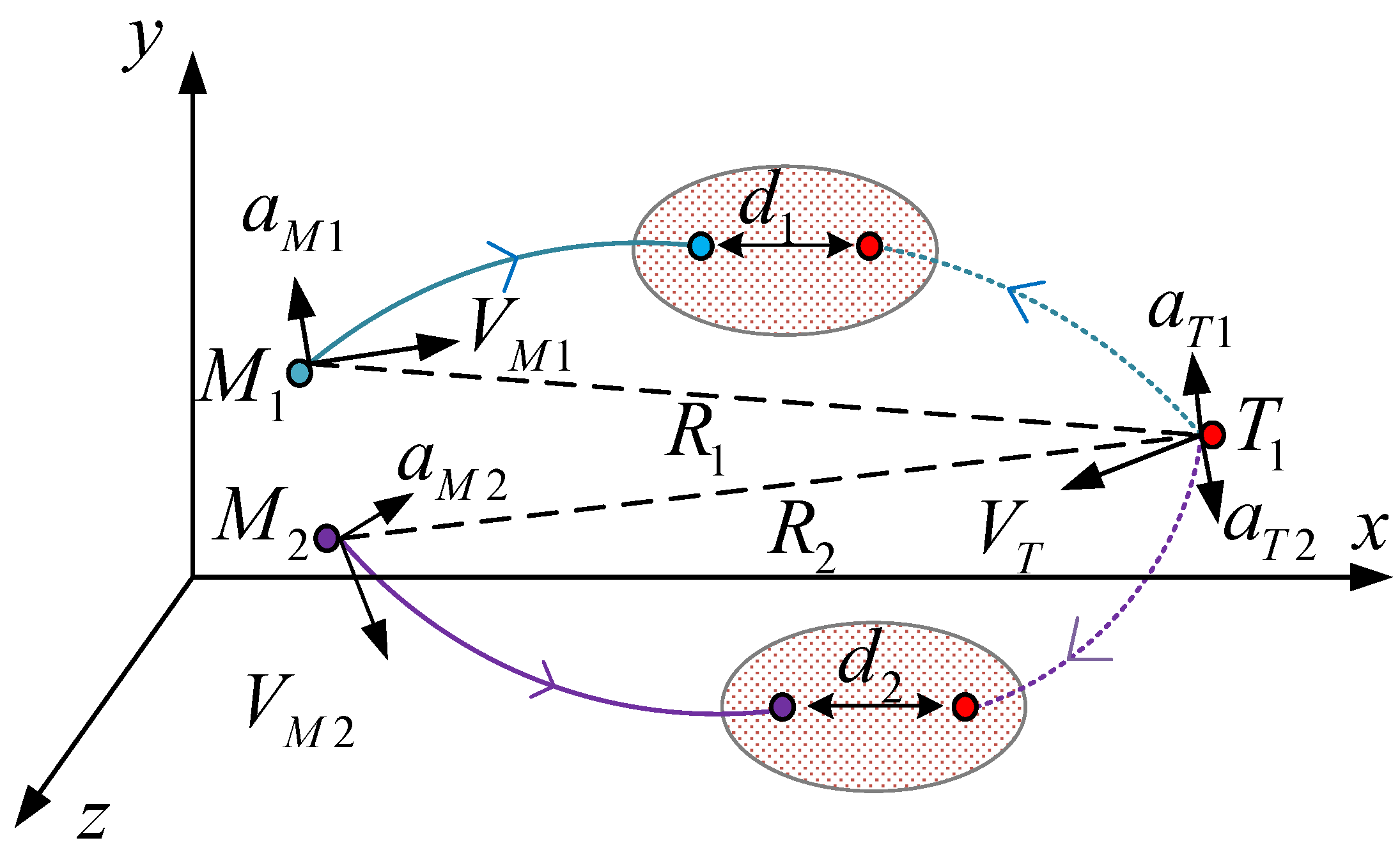
A schematic diagram of regional coverage interception is shown in Figure 1.

The main contributions of this paper are as follows:

1. Introduction of the Q-learning-cover regional coverage interception algorithm: This paper innovatively proposes the Q-learning-cover algorithm, combining regional coverage with time coordination. By integrating the geometric relationship between the pursuers and evaders and the coverage strategy of reinforcement learning, the algorithm increases the pursuit coverage area with each iteration in three-dimensional space, thus improving the pursuers’ interception efficiency.

2. Simplification of calculations using spherical-to-complex plane mapping: By introducing projection mapping, this paper projects the maneuvering range of the pursuers and evaders on a three-dimensional sphere onto the complex plane, simplifying arc surface calculations. This approach converts the coverage problem in three-dimensional space into a geometric mapping problem on the plane, significantly reducing computation complexity and improving the algorithm’s operability and efficiency.

3. Convergence analysis of the Q-learning-cover algorithm: Based on the assumption of iteration limits, this paper proves the convergence of the Q-learning-cover algorithm. By optimizing the iteration process, it ensures that pursuers can quickly find the optimal strategy to effectively cover and intercept the evader, guaranteeing convergence within a finite time.

In this paper, we propose a novel Q-learning-cover algorithm that combines geometric coverage in 3D space with temporal synchronization. Unlike traditional methods, our approach utilizes offline training of the Q-learning algorithm, where the model is trained in a simulation environment on various escapee motion patterns. Once trained, the model is then deployed online for the real-time guidance of the pursuers. This allows the system to leverage the computational efficiency of offline training while still enabling dynamic, online application during interception. The Q-learning algorithm is trained offline on a powerful computing platform, and the trained model is subsequently loaded onto the embedded hardware for online execution in real-world scenarios.

The structure of this paper is as follows: Section 2 describes the missile interception model in three-dimensional space; Section 3 discusses spherical-to-complex plane projection mapping for calculating the maneuvering range of pursuers and evaders; Section 4 presents the calculation method for interception time; Section 5 provides the update formula and iteration limit constraints for the Q-learning-cover algorithm; Section 6 presents the simulation platform used for missile interception. Section 7 shows numerical simulation and hardware-in-the-loop simulation experiments; Section 8 concludes the paper.

2. Dynamics Model

In the field of missile interception, the missile is considered as the pursuer, and the target is regarded as the evader. The pursuers $P_i$ cooperate to capture the and the evader $E_i$. This game takes place in three-dimensional space. It is assumed that both the pursuer and the evader are treated as particles with conventional acceleration constraints. The direction of velocity is adjusted by conventional acceleration, and the acceleration is always perpendicular to the direction of velocity. The motion model between the pursuer and the evader is shown in Figure 2. Based on the relationship between the pursuer $P_i$ and the evader $E_i$ in three-dimensional space, a nonlinear differential equation has been derived, as detailed in the study by Song et al. [49]. The model proposed in this paper forms the foundation for the models in the Figure 2.

$${\dot{R}}_{Pi}=v_{Ei}cos{\theta }_{Ei}cos{\phi }_{Ei}-v_{Pi}cos{\theta }_{Pi}cos{\phi }_{Pi}$$

(1)

$$R_{Pi}{\dot{\theta }}_{Li}=v_{Ei}sin{\theta }_{Ei}-v_{Pi}sin{\theta }_{Pi}$$

(2)

$$R_{Pi}{\dot{\phi }}_{Li}cos{\theta }_{Li}=v_{Pi}cos{\theta }_{Pi}sin{\phi }_{Pi}-v_{Ei}cos{\theta }_{Ei}sin{\phi }_{Ei}$$

(3)

$$\begin{array}{cc}\hfill {\dot{\theta }}_{Pi}=& {\displaystyle \frac{A_{yPi}}{v_{Pi}}}+tan{\theta }_{Li}sin{\phi }_{Pi}\times {\displaystyle \frac{(v_{Pi}cos{\theta }_{Pi}sin{\phi }_{Pi}-v_{Ei}cos{\theta }_{Ei}sin{\phi }_{Ei})}{R_{Pi}}}\hfill \\ \hfill & +cos{\phi }_{Pi}{\displaystyle \frac{(v_{Pi}sin{\theta }_{Pi}-v_{Ei}sin{\theta }_{Ei})}{R_{Pi}}}\hfill \end{array}$$

(4)

$$\begin{array}{cc}\hfill {\dot{\phi }}_{Pi}=& {\displaystyle \frac{A_{zPi}}{v_{Pi}cos{\theta }_{Pi}}}+sin{\theta }_{Pi}cos{\phi }_{Pi}tan{\theta }_{Li}+{\displaystyle \frac{v_{Ei}cos{\theta }_{Ei}sin{\phi }_{Ei}-v_{Pi}cos{\theta }_{Pi}sin{\phi }_{Pi}}{R_{Pi}cos{\theta }_{Pi}}}\hfill \\ \hfill & -sin{\theta }_{Pi}sin{\phi }_{Pi}{\displaystyle \frac{v_{Ei}sin{\theta }_{Ei}-v_{Pi}sin{\theta }_{Ei}}{R_{Pi}cos{\theta }_{Pi}}}-{\displaystyle \frac{v_{Ei}cos{\theta }_{Ei}sin{\phi }_{Ei}-v_{Pi}cos{\theta }_{Pi}sin{\phi }_{Pi}}{R_{Pi}}}\hfill \end{array}$$

(5)

$$\begin{array}{cc}\hfill {\dot{\theta }}_{Ei}=& {\displaystyle \frac{A_{yEi}}{v_{Ei}}}+tan{\theta }_{Li}sin{\phi }_{Ei}\ast {\displaystyle \frac{\left(v_{Pi}cos{\theta }_{Pi}sin{\phi }_{Pi}-v_{Ei}cos{\theta }_{Ei}sin{\phi }_{Ei}\right)}{R_{Pi}}}\hfill \\ \hfill & +cos{\phi }_{Ei}{\displaystyle \frac{\left(v_{Pi}sin{\theta }_{Pi}-v_{Ei}sin{\theta }_{Ei}\right)}{R_{Pi}}}\hfill \end{array}$$

(6)

$$\begin{array}{cc}\hfill {\dot{\phi }}_{Ei}=& {\displaystyle \frac{A_{zEi}}{v_{Ei}cos{\theta }_{Ei}}}+sin{\theta }_{Ei}cos{\phi }_{Ei}tan{\theta }_{Li}+{\displaystyle \frac{v_{Ei}cos{\theta }_{Ei}sin{\phi }_{Ei}-v_{Pi}cos{\theta }_{Pi}sin{\phi }_{Pi}}{R_{Pi}cos{\theta }_{Ei}}}\hfill \\ \hfill & -sin{\theta }_{Ei}sin{\phi }_{Ei}{\displaystyle \frac{v_{Ei}sin{\theta }_{Ei}-v_{Pi}sin{\theta }_{Ei}}{R_{Pi}cos{\theta }_{Ei}}}-{\displaystyle \frac{v_{Ei}cos{\theta }_{Ei}sin{\phi }_{Ei}-v_{Pi}cos{\theta }_{Pi}sin{\phi }_{Pi}}{R_{Pi}}}\hfill \end{array}$$

(7)

The pursuit–evasion problem in three-dimensional space is modeled as multiple pursuers attempting to capture an evader. The symbols used to describe the system dynamics are shown in

Table 1. Model parameters.

Symbol	Description	Coordinate System
$(X_I,Y_I,Z_I)$	Inertial reference coordinate system	Inertial system
$(X_L,Y_L,Z_L)$	Line-of-sight (LOS) coordinate system	Line-of-sight system
$(X_E,Y_E,Z_E)$	Velocity coordinate system of the i-th pursuer	Pursuer
$v_{Ei}$	Velocity of the i-th evader	Evader
$v_{Pi}$	Velocity of the i-th pursuer	Pursuer
$A_{Pi}$	Acceleration of the i-th pursuer	Pursuer
$A_{Ei}$	Acceleration of the i-th evader	Evader
${\gamma }_{Pi}$	Angle between the acceleration of the i-th pursuer and the $Y_{Pi}$ axis	Pursuer
${\gamma }_{Ei}$	Angle between the acceleration of the i-th evader and the $Y_E$ axis	Evader
$R_{Pi}$	Distance between the i-th pursuer and the evader	Inertial system
${\theta }_{Li}, {\phi }_{Li}$	Line-of-sight angles between the evader and the i-th pursuer relative to the inertial coordinate system	Line-of-sight system
${\theta }_{Pi}, {\phi }_{Pi}$	Elevation and inclination angles of $v_{Pi}$ relative to the line-of-sight system, starting from pointing at E	Pursuer
${\theta }_{Ei}, {\phi }_{Ei}$	Elevation and inclination angles of $v_{Ei}$ relative to the line-of-sight system, starting from pointing from $E_i$ to $P_i$	Evader
$A_{zPi}, A_{yPi}$	Projections of the normal accelerations along the $Z_{Pi}$ and $Y_{Pi}$ axes in the velocity coordinate system for the pursuer	Pursuer
$A_{zEi}, A_{yEi}$	Projections of the normal accelerations along the $Z_{Ei}$ and $Y_{Ei}$ axes in the velocity coordinate system for the evader	Evader

. In this paper, we default to using the Euclidean norm (2-norm) as the measure for norms. When other norms (e.g., infinity norm) are used, they will be explicitly indicated in the subscript.

3. Coverage Interception Based on Spherical Polar Projection Mapping

The coverage probability calculation method designed in this paper primarily involves calculating the intersection point of the velocity vector with the Ahlswede ball in space, which corresponds to the center of an ellipse. By using the current normal acceleration, we compute the components along the Y-axis and Z-axis in the velocity coordinate system, thereby determining the major and minor axes of the ellipse. When the normal acceleration is zero, a small positive number is used as a substitute to ensure the validity of the coverage probability calculation. We assume that the Ahlswede ball between the pursuer and the evader is as follows:

$$\begin{array}{cc}\hfill & {\left(x-{\displaystyle \frac{{\overline{x}}_P-{\lambda }_i^2{x}_E}{1-{\lambda }_i^2}}\right)}^2+{\left(y-{\displaystyle \frac{{\overline{y}}_P-{\lambda }_i^2{y}_E}{1-{\lambda }_i^2}}\right)}^2+{\left(z-{\displaystyle \frac{{\overline{z}}_P-{\lambda }_i^2{z}_E}{1-{\lambda }_i^2}}\right)}^2\hfill \\ \hfill & ={\displaystyle \frac{{\lambda }_i^2}{{\left(1-{\lambda }_i^2\right)}^2}}\left[{\left(x_E+{\overline{x}}_P\right)}^2+{\left(y_E+{\overline{y}}_P\right)}^2+{\left(z_E+{\overline{z}}_P\right)}^2\right]\hfill \end{array}$$

(8)

where ${\overline{x}}_P={\sum }_{i=1}^N{\gamma }_{Pxi}{x}_{Pi}, {\overline{y}}_P={\sum }_{i=1}^N{\gamma }_{Pyi}{y}_{Pi}, {\overline{z}}_P={\sum }_{i=1}^N{\gamma }_{Pzi}{z}_{Pi},$ ${\lambda }_i={\displaystyle \frac{∥{\mathbf{v}}_{Pi}∥}{∥{\mathbf{v}}_E∥}},$ Let $∥v_{Pi}∥$ represent the velocity of the pursuer in three-dimensional space and $∥v_E∥$ represent the velocity of the evader in three-dimensional space.

In this formula, we define the Apollonian sphere as the set of points in three-dimensional space that are bounded by a radius dependent on the velocities of both the pursuer and the evader. The variables $x,y,z$ represent the coordinates in space, while ${\overline{x}}_P,{\overline{y}}_P,{\overline{z}}_P$ are the weighted averages of the pursuer’s positions in three-dimensional space, given by the following summations:

We assume that the pursuer’s velocity vector in the inertial reference frame follows the line equation:

$$\begin{array}{cc}\hfill x_{Pi}^I& =x_{Pi}+v_x\Delta t\hfill \\ \hfill y_{Pi}^I& =y_{Pi}+v_y\Delta t\hfill \\ \hfill z_{Pi}^I& =z_{Pi}+v_z\Delta t\hfill \end{array}$$

where $x_{Pi},y_{Pi},z_{Pi}$ are the position coordinates of the pursuer, $v_x,v_y,v_z$ are the velocity components of the pursuer in three-dimensional space, and $\Delta t$ is the time step.

Spherical Polar Projection Mapping

When the pursuer’s velocity vector extends to the surface of the Ahlswede ball, it will cover the evader. To achieve this, we first need to allocate local coordinate systems on the sphere to describe the entire sphere through these local coordinate systems. This approach ensures that every point on the sphere has a unique corresponding coordinate. By combining these local coordinate systems, the entire sphere can be fully described. Next, we use spherical polar projection mapping to project these local regions from the three-dimensional real space onto a two-dimensional complex plane, as shown in Figure 3. Overlapping regions: The local coordinate systems of the coverage regions projected by different pursuers often overlap, leading to intersecting small areas. In these overlapping regions, we need to ensure that the local coordinate systems are correctly transformed to maintain consistency between different areas. Coverage of the sphere: Since the sphere is a closed surface, multiple local coordinate systems are required to cover the entire sphere. For example, on the unit sphere $S^2$ in three-dimensional space, multiple small regions can be formed through the pursuer’s region coverage, and a local coordinate system is defined for each small region. Ultimately, these local coordinate systems will work together to ensure maximum coverage of the area where the evader is located.

Select the coordinate system $OXYZ$ such that $OX$ and $OY$ coincide with the $Ox$ and $Oy$ axes on the complex plane and $ON$ is perpendicular to the complex plane, with $OZ$ aligned along the diameter $ON$. The complex number $I^{\ast }=x_I+y_{I}i$ corresponds to the point $(x_I,y_I)$, and the center of the sphere has coordinates $(x_E,y_E,z_E)$. We can calculate the coordinates of point N using the center of the sphere’s coordinates as follows:

$$\left({\displaystyle \frac{x_P-{\lambda }_i^2{x}_E}{1-{\lambda }_i^2}},{\displaystyle \frac{y_P-{\lambda }_i^2{y}_E}{1-{\lambda }_i^2}},{\displaystyle \frac{z_P-{\lambda }_i^2{z}_E}{1-{\lambda }_i^2}}\right)$$

(9)

This formula represents the calculation of the coordinates of point N in three-dimensional space, based on the center coordinates of the sphere $x_E,y_E,z_E$. The coordinates $x_P,y_P,z_P$ represent the position of point P, and ${\lambda }_i$ is an adjustment factor that scales the difference between point P and the sphere’s center. Specifically, ${\lambda }_i$ influences the variation in the coordinates $x_P,y_P,z_P$ in relation to the center of the sphere. The denominator $1-{\lambda }_i^2$ ensures the proper scaling and normalization of the coordinates, which is essential for maintaining the geometric relationships between the points in three-dimensional space. As ${\lambda }_i$ varies, the calculated coordinates of point N adjust accordingly, reflecting the influence of the center’s position and the relative distance between the points.

This formula represents the calculation of the coordinates of point N in three-dimensional space based on the sphere’s center coordinates $x_E,y_E,z_E$. The parameter ${\lambda }_i$ is an adjustment factor that influences the variation in $x_P,y_P,z_P$.

$$\left({\displaystyle \frac{x_P-{\lambda }_i^2{x}_E}{1-{\lambda }_i^2}},{\displaystyle \frac{y_P-{\lambda }_i^2{y}_E}{1-{\lambda }_i^2}},{\displaystyle \frac{z_P-{\lambda }_i^2{z}_E}{1-{\lambda }_i^2}}+{\displaystyle \frac{{\lambda }_i}{(1-{\lambda }_i^2)}}\sqrt{{(x_E+x_P)}^2+{(y_E+y_P)}^2+{(z_E+z_P)}^2}\right)$$

This equation calculates the new coordinates of point N by adding a correction term to the previous formula. The correction term ${\displaystyle \frac{{\lambda }_i}{(1-{\lambda }_i^2)}}$ is multiplied by the distance between the coordinates of the point P and the sphere’s center. The distance is represented by the Euclidean norm, which is the square root of the sum of the squared differences between the coordinates of the sphere center and point P. This term adjusts the calculated coordinates of point N, making it more accurate by accounting for the relative motion between the pursuer and evader.

Thus, the expression for the line $\overrightarrow{N{I}^{\ast }}$ is as follows:

$$\overrightarrow{N{I}^{\ast }}=\left(\begin{array}{cc}& {\displaystyle \frac{x_P-{\lambda }_i^2{x}_E}{1-{\lambda }_i^2}},\hfill \\ & {\displaystyle \frac{y_P-{\lambda }_i^2{y}_E}{1-{\lambda }_i^2}},\hfill \\ & {\displaystyle \frac{z_P-{\lambda }_i^2{z}_E}{1-{\lambda }_i^2}}-{\displaystyle \frac{{\lambda }_i}{(1-{\lambda }_i^2)}}\sqrt{{(x_E+x_P)}^2+{(y_E+y_P)}^2+{(z_E+z_P)}^2}\hfill \end{array}\right)$$

This formula describes the line equation $\overrightarrow{N{I}^{\ast }}$, which represents the relationship between point N and the complex number $I^{\ast }$. The coordinates $z_P,y_P,x_P$ are calculated based on the sphere’s center coordinates and the adjustment factor ${\lambda }_i$, which influences the geometry of the problem. The correction term is applied to the z-coordinate to account for the distance and improve the accuracy of the model.

Therefore, the line equation can be expressed as follows:

$$\begin{array}{cc}\hfill & {\displaystyle \frac{X-\frac{x_P-{\lambda }_i^2{x}_E}{1-{\lambda }_i^2}}{\frac{x_P-{\lambda }_i^2{x}_E}{1-{\lambda }_i^2}}}\hfill \\ \hfill & ={\displaystyle \frac{Y-\frac{y_P-{\lambda }_i^2{y}_E}{1-{\lambda }_i^2}}{\frac{y_P-{\lambda }_i^2{y}_E}{1-{\lambda }_i^2}}}\hfill \\ \hfill & ={\displaystyle \frac{Z-\frac{z_P-{\lambda }_i^2{z}_E}{1-{\lambda }_i^2}}{\frac{z_P-{\lambda }_i^2{z}_E}{1-{\lambda }_i^2}-\frac{{\lambda }_i}{(1-{\lambda }_i^2)}\sqrt{{(x_E+x_P)}^2+{(y_E+y_P)}^2+{(z_E+z_P)}^2}}}\hfill \end{array}$$

(10)

This represents the ratio form of the line equation, which is used to express the relationship between the points on the sphere and the complex plane. Each of the three equations in the ratio form corresponds to the normalized difference between the coordinates $X,Y,Z$ and the respective coordinates of the point N on the sphere. This form is essential for modeling the geometric relationship between the positions of the pursuer and the evader in three-dimensional space, ensuring that the calculations remain consistent and accurate.

To simplify subsequent calculations, we define the following:

$$\begin{array}{cc}\hfill X_c& ={\displaystyle \frac{x_P-{\lambda }_i^2{x}_E}{1-{\lambda }_i^2}},\hfill \\ \hfill Y_c& ={\displaystyle \frac{y_P-{\lambda }_i^2{y}_E}{1-{\lambda }_i^2}},\hfill \\ \hfill Z_c& ={\displaystyle \frac{z_P-{\lambda }_i^2{z}_E}{1-{\lambda }_i^2}},\hfill \\ \hfill B_r& ={\displaystyle \frac{{\lambda }_i}{(1-{\lambda }_i^2)}}\sqrt{{(x_E+x_P)}^2+{(y_E+y_P)}^2+{(z_E+z_P)}^2}\hfill \end{array}$$

Here, we define new variables $X_c,Y_c,Z_c$, and $B_r$ to simplify the subsequent calculations. These variables are derived from the previous expressions for the coordinates of point N and the correction term. The variables $X_c,Y_c,Z_c$ represent the adjusted coordinates of point P, while $B_r$ represents a correction factor that accounts for the distance between the points on the sphere. By introducing these simplified variables, we reduce the complexity of the formulas and make the upcoming steps in the calculation more manageable.

At this point, the line equation can be rewritten as follows:

$${\displaystyle \frac{X-X_c}{x-X_c}}={\displaystyle \frac{Y-Y_c}{y-Y_c}}={\displaystyle \frac{Z-Z_c-B_r}{-Z_c-B_r}}$$

(11)

This represents the simplified form of the line equation, using $X_c,Y_c,Z_c, B_r$ to represent the parameters of the line. By expressing the equation in terms of these new variables, we streamline the process of calculating the corresponding points on the sphere and the complex plane. The simplified equation reduces the complexity and allows for easier manipulation in subsequent calculations.

We can express the correspondence between points on the sphere and points on the complex plane as follows:

$$x={\displaystyle \frac{(X-X_c)(-Z_c-B_r)}{Z-Z_r-B_r}}+X_c$$

$$y={\displaystyle \frac{(Y-Y_c)(-Z_c-B_r)}{Z-Z_c-B_r}}+Y_c$$

These formulas illustrate the correspondence between points on the sphere and points on the complex plane. They provide the relationships between the coordinates $x,y$ on the complex plane and the corresponding coordinates $X,Y$ on the sphere, adjusted by the values of $X_c,Y_c,Z_c,B_r$. This correspondence is crucial for converting between the two coordinate systems and analyzing their geometric relationship.

Furthermore, the correspondence between points on the complex plane and points on the sphere is given by the following:

$$\begin{array}{cc}\hfill Z& ={\displaystyle \frac{({(x-X_c)}^2+{(y-Y_c)}^2)\left((Z_c+B_r)\right)-\left({(Z_r+B_r)}^2\right)(B_r-Z_c)}{{(x-X_c)}^2+{(y-Y_c)}^2+{(Z_c+B_r)}^2}},\hfill \\ \hfill X& ={\displaystyle \frac{({(x-X_c)}^2+{(y-Y_c)}^2)\left((Z_c+B_r)\right)-\left({(Z_r+B_r)}^2\right)(B_r-Z_c)}{({(x-X_c)}^2+{(y-Y_c)}^2+{(Z_c+B_r)}^2)(-Z_c-B_r)}}+(x-X_c)+X_c,\hfill \\ \hfill Y& ={\displaystyle \frac{({(x-X_c)}^2+{(y-Y_c)}^2)\left((Z_c+B_r)\right)-\left({(Z_r+B_r)}^2\right)(B_r-Z_c)}{({(x-X_c)}^2+{(y-Y_c)}^2+{(Z_c+B_r)}^2)(-Z_c-B_r)}}+(y-Y_c)+Y_c\hfill \end{array}$$

(12)

These formulas provide expressions for solving the $X,Y,Z$ coordinates on the sphere based on the known $x,y$ coordinates on the complex plane. They demonstrate the precise relationship between the sphere and the complex plane, allowing for the conversion between the two coordinate systems. These equations are essential for mapping the points on the sphere to the complex plane and vice versa, which is key to understanding the geometric relationship between the two systems.

Through spherical polar projection, a circle not passing through point N is mapped to a circle on the complex plane. Suppose the equation of the spherical circle is

$$A(X^2+Y^2+Z^2)+CX+DY+EZ+G=0,(A\ne 0)$$

(13)

The equation of the circle on the complex plane can be written as

$$a{(x-x_I)}^2+b{(y-y_I)}^2+c=0,(a,b\ne 0)$$

(14)

This equation is used to represent the relationship between the circle on the sphere and the circle on the complex plane. In the simulation process, by solving the system of equations, we obtain the expressions for each parameter, which leads to the equation of the circle on the complex plane.

By solving the Ahlswede ball equation and the line equation, we obtain the intersection points of the pursuer $\left[x_{Pi}^I,y_{Pi}^I,z_{Pi}^I\right]$ and the evader $\left[x_E^I,y_E^I,z_E^I\right]$. Based on this, the normal accelerations of both parties serve as the major and minor axes of two ellipses. We then project these two ellipses onto the complex plane and calculate their intersection points. For the intersection points of these two ellipses, there are two possible cases. The first case is shown in Figure 4, and the second case is shown in Figure 5.

The projection plane represents the projection of the current player’s information onto the $X-Z$ plane in the inertial frame, which facilitates the calculation of the coverage area. The choice of the projection plane is related to the distance between the pursuer and the evader. The projection plane in the inertial system is parallel to the $Y_I-Z_I$ plane, with the $X_I$-axis given by

$$X_I\left[{\displaystyle \frac{1}{\alpha }}\left({\displaystyle \frac{1}{n}}\sum _{i=1}^n{x}_{P_i}+x_E\right)\right]$$

Circle $C_E$ represents the maximum normal cutoff coverage area of the evader E, where the center of the circle is the optimal game point of the evader $I_E^{\ast }=(x_E^{\ast },y_E^{\ast },z_E^{\ast })$, and the radius is the maximum normal cutoff $a_E^{\max }$ of the evader.

Ellipse $E_E$ represents the current normal cutoff coverage area of the evader, with the two axes of the ellipse defined as follows: $a_E^Y$ is the normal acceleration along the Y-axis in the evader’s velocity system, and $a_E^Z$ is the normal acceleration along the Z-axis in the evader’s velocity system. The center of the ellipse $E_E$ is the same as the center of circle $C_E$.

Ellipse $E_{P_i}$ represents the normal cutoff coverage area of the pursuer $P_i$. The center of the ellipse $E_{P_i}$ is the optimal game point of the pursuer $I_{P_i}^{\ast }=(x_{P_i}^{\ast },y_{P_i}^{\ast },z_{P_i}^{\ast })$, and the two axes of the ellipse $E_{P_i}$ are set as follows: $a_{P_i}^Y$ is the normal acceleration along the Y-axis in the pursuer’s velocity system, and $a_{P_i}^Z$ is the normal acceleration along the Z-axis in the pursuer’s velocity system.

The coverage areas of the pursuer and evader intersect at four focal points. This is simply for illustrative purposes, and different forms of the focal points will be given later. The intersection points $I_1$ and $I_3$ represent the intersections of the current acceleration coverage areas of the pursuer and evader. The coverage area $S_1$ is formed by the trajectory from $I_1$ to the lower trajectory $I_3$. The intersection points $I_2$ and $I_4$ represent the intersections of the current velocity coverage area of the pursuer and the maximum velocity coverage area of the evader. The coverage area $S_2$ is formed by the trajectory from $I_3$ to the lower trajectory $I_4$.

4. Calculation of Interception Time

In this section, we first introduce a method for calculating the interception time in two-dimensional space. Based on this, we extend the method to three-dimensional space and propose a method for calculating interception time under three-dimensional conditions. Additionally, we design a guidance method based on time deviation, which uses a variable proportional coefficient to adjust the proportional guidance rate.

The schematic diagram of the synchronous interception of two-to-one missiles is shown in Figure 6. $d_1,d_2$ represent the set flight ranges of the missiles at their termination time. We use two missiles intercepting two virtual motions of the target simultaneously, where these two virtual points are defined at the initial moment. Apart from the acceleration, all other initial parameters are the same. In this way, two missiles can intercept the same batch of targets, thus achieving batch interception. If the two missiles can pass the acceleration determination values to the virtual point commands of the same batch of targets, it can be assumed that when one missile reaches its maximum acceleration, both missiles can successfully intercept the target. This way, a complex interception of the target can be achieved.

As shown in Figure 6, during the interception process, the missiles are modeled using virtual points. This method can effectively simplify the complex interaction between the missile and the target. Next, we will derive more detailed expressions based on these models and use mathematical formulas to optimize the interception time and path planning.

Lemma 1.

The launch time of a missile intercepting a moving target in two-dimensional space is given by [23]

$$t_{goS}={\displaystyle \frac{1}{K_b}}\left({\displaystyle \frac{\alpha \left|{\sigma }_M^{\alpha +3}\left(0\right)\right|}{6(\alpha +3)}}-{\displaystyle \frac{\left|{\sigma }_M^{\alpha +1}\left(0\right)\right|}{\alpha +1}}\right)$$

(15)

$$\Delta t_{go}={\displaystyle \frac{V_{MF}\left(t_{goS}\right)·(t_{goF}-t_{goS})}{V_{MR}\left(t_{goS}\right)-V_{T}cos{\sigma }_{TF}\left(0\right)}}$$

(16)

$$t_{go}=t_{goS}+\Delta t_{go}$$

(17)

where ${\sigma }_M$ is the angle between the missile’s velocity system and the line-of-sight system; $t_{goF}$ is the forward time of missile attack on the virtual stationary target $T_{Ff}$ calculated by the PN guidance law; $K_b$ is a constant related to the viewing angle; α is a constant related to the proportional coefficient, and $\alpha =-{\displaystyle \frac{N-2}{N-1}}$; N is the proportional coefficient.

When calculating interception time in three-dimensional space, we improve Lemma 1. First, we calculate the attack time $t_{goLi}$ of the missile along a straight path. Then, compared to the two-dimensional case, the interception time calculation in three-dimensional space must consider the influence of the z-axis. For the straight path, the calculation process is as follows:

$$t_{goLi}={\displaystyle \frac{1}{v_{Mi}}}\sqrt{\begin{array}{c}{[x_{Ti}\left(t_{goLi}\right)-x_{Mi}\left(0\right)]}^2\hfill \\ +{[y_{Ti}\left(t_{goLi}\right)-y_{Mi}\left(0\right)]}^2\hfill \\ +{[z_{Ti}\left(t_{goLi}\right)-z_{Mi}\left(0\right)]}^2\hfill \end{array}}$$

(18)

The equation for $t_{goLi}$ can be derived as

$$\begin{array}{cc}\hfill & \left[v_{Ti}^2-v_{Mi}^2+a_{Tiz}\left(z_{Ti}-z_{Mi}\right)+a_{Tiy}\left(y_{Ti}-y_{Mi}\right)\right]t_{goLi}^2\hfill \\ \hfill & +2v_{Ti}\left(y_{Ti}-y_{Mi}\right)t_{goLi}+R_0^2=0\hfill \end{array}$$

(19)

Next, the time required for the missile to attack along the straight path is calculated as follows:

$$t_{goLi}={\displaystyle \frac{\left(-n-\sqrt{n^2-4{\dot{R}}_i^{2m_i}}\right)}{2m_i}}$$

(20)

where ${\dot{R}}_i$ is the derivative of the distance between the target and the missile. The expression for $m_i$ is

$$m_i=v_{Mi}^2-v_{Ti}^2+a_{Tiy}\Delta y+a_{Tiz}\Delta z,$$

where $a_{Tiy}$ is the component of the target’s velocity along the Y-axis in the target velocity coordinate system. Additionally, the value of n is

$$n=2v_{Ti}\Delta x$$

where $\Delta x_i$ represents the distance between the target and the missile. Next, we calculate the time required for the missile to reach the virtual point. After determining the attack time $t_{goLi}$ along the straight line, we assume the target moves to a virtual point $T{F}_V$ in the velocity coordinate system. Through the transformation matrix, we can obtain the position of the virtual point $TF$ in the ground reference system, thus calculating the terminal velocity of the target. The missile’s speed is then converted to the virtual line-of-sight system. At the virtual target point, the angles ${\theta }_{MiF}$ and ${\phi }_{MiF}$ represent the angle between the missile’s line-of-sight system and velocity system, and ${\theta }_{TiF}$ and ${\phi }_{TiF}$ represent the angle between the target’s velocity system and the line-of-sight system. The angles ${\sigma }_{MiF}$ and ${\sigma }_{TiF}$ are calculated as follows:

$${\sigma }_{MiF}=arccos\left(cos\left({\theta }_{MiF}\right)cos\left({\phi }_{MiF}\right)\right)$$

(21)

$${\sigma }_{TiF}=arccos\left(cos\left({\theta }_{TiF}\right)cos\left({\phi }_{TiF}\right)\right)$$

(22)

The angles ${\sigma }_{MiF}$ and ${\sigma }_{TiF}$ are intermediate variables and do not have actual physical meaning. The time for the missile to reach the virtual position is given by

$$\begin{array}{cc}\hfill & t_{goFi}={\displaystyle \frac{\left(-{\left|{\sigma }_{MiF}\right|}^{\alpha +1}\right)}{\alpha +1}}+{\displaystyle \frac{\alpha {\left|{\sigma }_{MiF}\right|}^{\alpha +3}}{6\left(\alpha +3\right)}}\hfill \\ \hfill & \begin{array}{cc}& \end{array}+{\displaystyle \frac{K_a{\left|{\sigma }_{MiF}\right|}^{\alpha +2}}{\alpha +2}}-K_a{\displaystyle \frac{\alpha {\left|{\sigma }_{MiF}\right|}^{\alpha +4}}{6\left(\alpha +4\right)}}\hfill \end{array}$$

(23)

where $R_{Fi}$ is the distance between the missile and the virtual point.

The constant $K_b={\displaystyle \frac{-\left(N-1\right)v_{Mi}{\left(\left|sin\left({\sigma }_{MiF}\right)\right|\right)}^{\frac{1}{N-1}}}{R_{Fi}{e}^{K_a\left|{\sigma }_{MiF}\right|}}}$ represents a constant related to the missile’s velocity and the angle ${\sigma }_{MiF}$, where $v_{Mi}$ is the missile’s velocity, $R_{Fi}$ is the distance from the missile to the virtual point, and $K_a$ is the missile’s lift-to-drag ratio constant.

The constant $K_a={\displaystyle \frac{N}{N-1}}yta$, where $yta$ is the missile’s lift-to-drag ratio.

The deviation time can be calculated as

$$\Delta t_{goi}={\displaystyle \frac{v_{MiT}{t}_{di}}{v_{MiT}\left(v_{MiT}-cos\left({\sigma }_{TiF}\right)v_{Ti}\right)}}$$

(24)

where $\mathsf{\Xi }={\displaystyle \frac{ytaNsin\left({\sigma }_{MiF}\right)\left(0-{\sigma }_{MiF}\right)}{N-1}}$ represents a term involving the missile’s lift-to-drag ratio, the proportional coefficient N, and the angle ${\sigma }_{MiF}$.

The missile’s velocity after correction is given by $v_{MiT}=v_{Mi}{e}^{\mathsf{\Xi }}$, where $v_{Mi}$ is the missile’s initial velocity and $\mathsf{\Xi }$ is a correction factor based on the missile’s lift-to-drag ratio.

Additionally, $t_{di}=t_{goFi}-t_{goLi}$, where $t_{goFi}$ is the forward time for missile attack, and $t_{goLi}$ is the time to reach a stationary target.

In Lemma 1, during each iteration, we consider a stationary target. However, in this paper, we need to consider the target’s movement with random acceleration. Therefore, we need to subtract the target’s movement impact from the time calculated in each iteration.

$$\Delta t_{goTi}=-{\displaystyle \frac{\sqrt{\begin{array}{c}{[x_{Ti}\left(t+t_{goLi}\right)-x_{Ti}\left(t\right)]}^2\hfill \\ +{[y_{Ti}\left(t+t_{goLi}\right)-y_{Ti}\left(t\right)]}^2\hfill \\ +{[z_{Ti}\left(t+t_{goLi}\right)-z_{Ti}\left(t\right)]}^2\hfill \end{array}}}{\left(\begin{array}{c}{v}_{Ti}cos{\theta }_{Ti}\left(t+t_{goLi}\right)cos{\phi }_{Ti}\left(t+t_{goLi}\right)\hfill \\ -v_{Ti}cos{\theta }_{Ti}\left(t\right)cos{\phi }_{Ti}\left(t\right)\hfill \end{array}\right)}}$$

(25)

where t is the current time and $t_{goSi}$ is the interception time.

$$t_{goSi}=t_{goLi}+\Delta t_{goi}+\Delta t_{goTi}$$

(26)

The difference between the current estimated interception time and the actual interception time can be obtained. $t_{errori}$ is the error time, $i=1,2$.

$$t_{errori}=t_{goi}-t_{goSi}$$

(27)

In the aforementioned methods for calculating coverage probability and interception time, we primarily focus on the spatial relationship and coverage probability between the pursuer and the evader. However, this is a static analysis of the pursuit–evasion game, while in practice, the behavior of the pursuer and the evader is dynamic and there are strategic interactions between them. To address this complex dynamic game, we introduce the Q-learning-cover algorithm.

The Q-learning-cover algorithm uses reinforcement learning to train the strategies of the pursuer and evader, combining area cover and time coordination problems to optimize the solution to the pursuit–evasion game. The key to this algorithm is to gradually optimize the strategy through Q-value updates, so that the pursuer maximizes the probability of capturing the evader, while the evader tries to escape the pursuit by adjusting its strategy. Through this method, the Q-learning-cover algorithm not only considers the actions of both parties in the game but also effectively adapts to the changing game environment.

Next, we will provide a detailed introduction to the design and implementation of the Q-learning-cover algorithm and analyze its application effectiveness in the pursuit–evasion game.

5. Q-Learning-Cover Algorithm

In this section, we present the Q-learning-cover algorithm, which is based on the previously described coverage probability calculation method. The algorithm trains both the pursuer and the evader separately, thereby solving the pursuit–evasion game. In the pursuit–evasion game, the actions of the pursuer and evader are interdependent. Therefore, both must be trained individually to allow the model to effectively learn how to make optimal decisions based on real-time states and environments.

The Q-learning-cover algorithm combines the Q-learning algorithm from reinforcement learning with the concept of area cover. By iteratively training the behavior of each participant (the pursuer and the evader), the strategy is gradually optimized. Specifically, the goal of the pursuer is to maximize the probability of capturing the evader by continuously adjusting its behavior, while the evader tries to adjust its strategy to maximize its chances of escaping the pursuit.

In this algorithm, the training of the reinforcement learning model considers not only the actions of the participants but also integrates the area coverage probabilities and the synergistic effects of both parties’ behaviors at different points in time. The specific training process gradually improves the expected return of each participant in each state by updating the Q-values. To achieve this, the Q-learning-cover algorithm incorporates area coverage and time factors into the Q-value updating process, forming a bilateral game strategy.

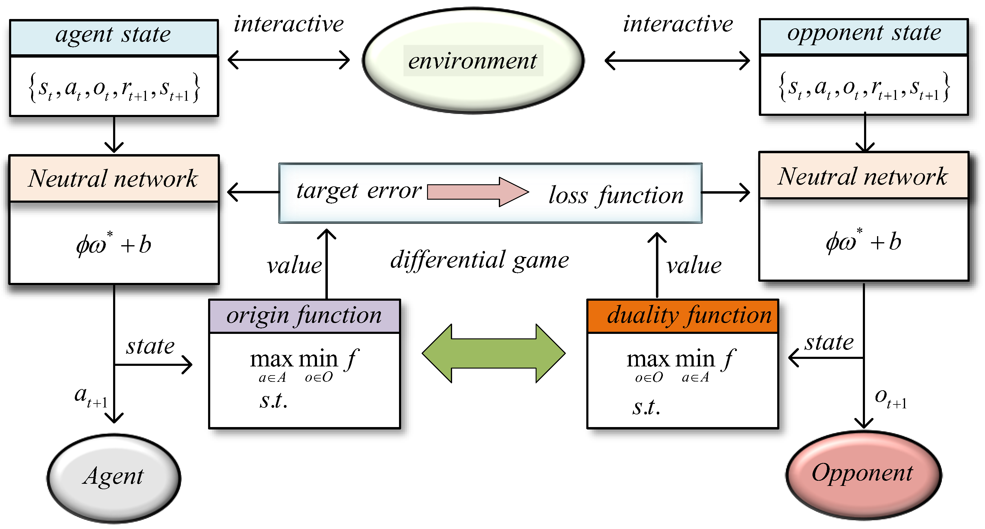
Figure 7 shows the game strategy of the Q-learning-cover algorithm. On the left side is the strategy diagram for the pursuer, and on the right side is the strategy diagram for the evader. The two interact in different game states and adjust according to the feedback from reinforcement learning. Through this method, both the pursuer and evader can find the optimal pursuit–evasion strategy in complex environments.

By incorporating area coverage and time coordination, the Q-learning-cover algorithm is able to provide a more accurate solution to the pursuit–evasion game in dynamic environments. The behavior patterns of both the pursuer and the evader are continuously optimized during the training process, eventually reaching the optimal strategy. This enables the algorithm to effectively address complex pursuit–evasion problems encountered in real-world applications. The update formula for Q-learning-cover is shown below:

The Q-learning-cover algorithm is designed to efficiently plan the trajectories of multiple pursuers to intercept a single evader. The following pseudo-code outlines the main steps of the algorithm, incorporating both the interception time and regional coverage calculation before the algorithm iterations begin. Algorithm 1 shows the steps of the Q-learning-cover algorithm.

Algorithm 1 Q-learning-cover algorithm

1: Initialize the state space S, action space A, and Q-table $Q(s,a)$   2: Set learning parameters: $\alpha$ (learning rate), $\gamma$ (discount factor), and $ϵ$ (exploration rate)   3: (Interception Time Calculation)   4: Calculate the interception time $t_{intercept}$ based on the positions and velocities of pursuers and the evader.   5: (Regional Coverage Calculation)   6: Calculate the regional coverage based on the positions of the pursuers and the evader’s trajectory, using geometric covering techniques such as the Ahlswede sphere.   7: for each episode do   8:     Initialize the environment (pursuer and evader positions)   9:     while not converged do 10:         Select action a using an epsilon-greedy policy: $a=arg{max}_{a}Q(s,a)$ 11:         Execute action a and observe new state $s^{\prime }$ and reward r 12:         Update Q-value using the formula:                       $Q(s,a)\leftarrow Q(s,a)+\alpha (r+\gamma {\displaystyle \underset{a^{\prime }}{max}}Q(s^{\prime },a^{\prime })-Q(s,a))$ 13:     end while 14: end for 15: Return the optimized policy

Theorem 1.

When the Q-learning-cover algorithm satisfies the selection upper bound condition in Equation (28), then convergence is achieved.

$$\begin{array}{cc}\hfill & {\displaystyle \frac{1}{N}}\sum _{t=0}^{N-1}E\left[\parallel Q_t-Q^{\ast }{\parallel }_{\infty }\right]\le \left({\displaystyle \frac{1-\rho }{1+\rho }}\right)\hfill \\ \hfill & \times \left[\left({\displaystyle \frac{1}{N}}\sum _{t=0}^{N-1}E\left[\parallel Q_t-Q^{\ast }{\parallel }^2\right]\right)+{\gamma }^2{\left({\displaystyle \frac{R_{\mathit{max}}}{1-\gamma }}\right)}^2+{\displaystyle \frac{1}{N}}\sum _{t=0}^{N-1}E\left[\parallel {\pi }_t-{\pi }^{\ast }{\parallel }^2\right]\right]\hfill \end{array}$$

(28)

-

${\displaystyle \frac{1}{N}}{\sum }_{t=0}^{N-1}E\left[\parallel Q_t-Q^{\ast }{\parallel }_{\infty }\right]$: This term represents the average error in the Q-values over N iterations. $Q_t$ is the Q-value at time t, and $Q^{\ast }$ is the optimal Q-value. The error is measured using the infinity norm (${\parallel ·\parallel }_{\infty }$), which refers to the maximum difference between the current Q-values and the optimal Q-values. This term gives the expected error across all iterations.

-

$\left({\displaystyle \frac{1-\rho }{1+\rho }}\right)$: This factor is the convergence rate. It ensures that as the algorithm progresses, the error decreases over time. The parameter $\rho$ controls how quickly the algorithm converges—lower values of $\rho$ result in faster convergence.

-

$\left({\displaystyle \frac{1}{N}}{\sum }_{t=0}^{N-1}E\left[\parallel Q_t-Q^{\ast }{\parallel }^2\right]\right)$: This term is the second moment of the error. It measures the average squared error of the Q-values. The second moment provides a more detailed view of how the error evolves over time, which is crucial for understanding the stability of the algorithm.

-

${\gamma }^2{\left({\displaystyle \frac{R_{\max }}{1-\gamma }}\right)}^2$: This term accounts for the discount factor $\gamma$, which determines how much weight is given to future rewards. $R_{\max }$ represents the maximum reward, and this term adjusts the impact of future rewards on the convergence.

-

${\displaystyle \frac{1}{N}}{\sum }_{t=0}^{N-1}E\left[\parallel {\pi }_t-{\pi }^{\ast }{\parallel }^2\right]$: This is the policy error, which measures how far the current policy ${\pi }_t$ deviates from the optimal policy ${\pi }^{\ast }$. This term represents the gap between the learned policy and the optimal policy.

This theorem shows that the Q-learning-cover algorithm will converge to the optimal Q-values and optimal policy as long as the algorithm satisfies the upper bound condition specified in Equation (28). The convergence is guaranteed by controlling the Q-value error, policy error, and the impact of future rewards through the discount factor $\gamma$. Each term on the right-hand side of the equation ensures that as the algorithm progresses, the error will decrease, ultimately leading to convergence.

Proof. 

Our proof starts from the following elementary analysis and inverse recursion formula:

$$\begin{array}{c}{\Delta }_t=Q_t-Q^{\ast }\hfill \\ =\left(I-{\mathsf{\Lambda }}_t\right)Q_{t-1}+{\mathsf{\Lambda }}_t\left(r+\gamma P_t{\pi }_t+\beta {\tilde{O}}_t+\mu {\tilde{T}}_t\right)-Q^{\ast }\hfill \\ =\left(I-{\mathsf{\Lambda }}_t\right)\left(Q_{t-1}-Q^{\ast }\right)+{\mathsf{\Lambda }}_t\left(r+\gamma P_t{\pi }_t+\beta {\tilde{O}}_t+\mu {\tilde{T}}_t-Q^{\ast }\right)\hfill \\ =\left(I-{\mathsf{\Lambda }}_t\right)\left(Q_{t-1}-Q^{\ast }\right)+\gamma {\mathsf{\Lambda }}_t\left(P_t{\pi }_t-{P\pi }^{\ast }\right)+{\mathsf{\Lambda }}_t\left(\beta {\tilde{O}}_t+\mu {\tilde{T}}_t\right)\hfill \\ =\left(I-{\mathsf{\Lambda }}_t\right){\Delta }_{t-1}+\gamma {\mathsf{\Lambda }}_t\left(P_t-P\right){\pi }^{\ast }+\gamma {\mathsf{\Lambda }}_t{P}_t\left({\pi }_t-{\pi }^{\ast }\right)+{\mathsf{\Lambda }}_t\left(\beta {\tilde{O}}_t+\mu {\tilde{T}}_t\right)\hfill \\ =A{\Delta }_{t-1}+\gamma {\mathsf{\Lambda }}_t\left(P_t-P\right){\pi }^{\ast }+\gamma {\mathsf{\Lambda }}_t{P}_t\left({\pi }_t-{\pi }^{\ast }\right)+{\mathsf{\Lambda }}_t\left(\beta {\tilde{O}}_t+\mu {\tilde{T}}_t\right)\hfill \end{array}$$

(29)

where for any $t>0$, the first line comes from the update rule of the Q-learning algorithm, which computes the Q-value update based on the previous Q-value, the reward, and the transition probabilities. The term $Q_t$ is the current Q-value, and $Q^{\ast }$ is the optimal Q-value. The second-to-last line comes from the Bellman equation, which represents the optimal Q-value function as $Q^{\ast }=r+\gamma P{\pi }^{\ast }$ [17], where r is the reward, $\gamma$ is the discount factor, P is the transition probability matrix, and ${\pi }^{\ast }$ is the optimal policy. The Bellman equation is used to express the recursive relationship between the Q-values, the reward, and the future state values.

We assume that

$$\begin{array}{c}{∥A∥}_{\infty }:={max}_{1\le i\le m}{\sum }_{j=1}^n\left|A_{ij}\right|\hfill \\ ={max}_{1\le i\le m}{\displaystyle \sum _j}\left|{\left[A\right]}_{ij}\right|\hfill \\ ={max}_{1\le i\le m}{\displaystyle \sum _j}\left|I-{\mathsf{\Lambda }}_t\right|\hfill \\ =\underset{1\le i\le m}{max}\left(1-\eta \right)\hfill \\ \le \rho \hfill \end{array}$$

In this formula, we are defining the infinity norm of a matrix A, which is calculated by taking the maximum of the row sums of the absolute values of the elements. The first line expresses the definition of the infinity norm for matrix A. The second line represents the same norm, expressed in terms of the elements of matrix A, where $A_{ij}$ is the element in the i-th row and j-th column of the matrix. In the third line, we use the identity $I-{\mathsf{\Lambda }}_t$, which is a difference between the identity matrix and a matrix ${\mathsf{\Lambda }}_t$, and the absolute values of its elements are summed to calculate the norm. The fourth line assumes that the maximum of these sums is bounded by $1-\eta$, where $\eta$ is a parameter. Finally, the last line indicates that the norm is bounded by a constant $\rho$, which is a convergence parameter. This bound ensures that the norm does not grow unbounded as the algorithm proceeds.

Next, we design the Lyapunov function $V\left(x\right)=x^{T}Mx$, where for any $\epsilon >0$, $\rho +\epsilon \in (0,1)$. We assume the existence of a positive definite matrix $M\succ 0$, such that

$$A^{T}MA={\left(\rho +\epsilon \right)}^2\left(M-I\right)$$

and

$${\lambda }_{min}\left(M\right)\ge 1,$$

$${\lambda }_{max}\left(M\right)\le {\displaystyle \frac{\left|S\right|\left|A\right|}{1-{\left(\frac{\rho }{\rho +\epsilon }\right)}^2}}.$$

In this part of the proof, we define a Lyapunov function $V\left(x\right)=x^{T}Mx$, where M is a positive definite matrix. The Lyapunov function is a key tool in proving stability and convergence of dynamic systems. The term $x^{T}Mx$ ensures that the energy-like quantity is non-negative and decreases over time. We introduce a condition on the matrix M such that it is positive definite ($M\succ 0$), ensuring that M has strictly positive eigenvalues. The first equation $A^{T}MA={(\rho +\epsilon )}^2(M-I)$ defines a relationship between M, the matrix A, and the identity matrix I, where $\rho +\epsilon$ is a factor controlling the contraction or expansion behavior of the system. The second inequality ${\lambda }_{min}\left(M\right)\ge 1$ states that the minimum eigenvalue of M is greater than or equal to 1, ensuring that the matrix is not degenerate and that the Lyapunov function behaves correctly. The third inequality ${\lambda }_{max}\left(M\right)\le {\displaystyle \frac{\left|S\right|\left|A\right|}{1-{\left(\frac{\rho }{\rho +\epsilon }\right)}^2}}$ provides an upper bound on the maximum eigenvalue of M. This bound is critical in determining the stability of the system, as it ensures that M does not grow too large, maintaining the desired convergence properties.

Then, by substituting these formulas into the Lyapunov function, we can obtain

$$\begin{array}{c}E\left[V\left({\Delta }_{t+1}\right)\right]\hfill \\ =E\left[{\left(A{\Delta }_t+\gamma {\mathsf{\Lambda }}_{t+1}\left(P_{t+1}{\pi }_t-P{\pi }^{\ast }\right)+{\mathsf{\Lambda }}_t\left(\beta {\tilde{O}}_t+\mu {\tilde{T}}_t\right)\right)}^{T}M\right.\hfill \\ \left.\left(A{\Delta }_t+\gamma {\mathsf{\Lambda }}_{t+1}\left(P_{t+1}{\pi }_{t+1}-P{\pi }^{\ast }\right)+{\mathsf{\Lambda }}_t\left(\beta {\tilde{O}}_t+\mu {\tilde{T}}_t\right)\right)\right]\hfill \\ ={\Delta }_t^T{A}^{T}MA{\Delta }_t+{\gamma }^2{\left(P_{t+1}{\pi }_t-P{\pi }^{\ast }\right)}^T{\mathsf{\Lambda }}_{t+1}^{T}M{\mathsf{\Lambda }}_{t+1}\hfill \\ \left(P_{t+1}{\pi }_{t+1}-P{\pi }^{\ast }\right)+{\beta }^2{\tilde{O}}_t^T{\mathsf{\Lambda }}_{t+1}^{T}M{\mathsf{\Lambda }}_{t+1}{\tilde{O}}_t+{\mu }^2{\tilde{T}}_t^T{\mathsf{\Lambda }}_{t+1}^{T}M{\mathsf{\Lambda }}_{t+1}{\tilde{T}}_t\hfill \\ <{(\rho +\epsilon )}^2{\Delta }_t^T(M-I){\Delta }_t+{\gamma }^2{\left(P_{t+1}{\pi }_t-P{\pi }^{\ast }\right)}^T{\mathsf{\Lambda }}_{t+1}^{T}M{\mathsf{\Lambda }}_{t+1}\hfill \\ \left(P_{t+1}{\pi }_{t+1}-P{\pi }^{\ast }\right)+{\eta }^2\left({\beta }^2{\tilde{O}}_t^T{\tilde{O}}_t+{\mu }^2{\tilde{T}}_t^T{\tilde{T}}_t\right){\lambda }_{max}\left(M\right)\hfill \\ <{(\rho +\epsilon )}^{2}V\left({\Delta }_t\right)-{(\rho +\epsilon )}^2{\parallel {\Delta }_t\parallel }^2+{\gamma }^2{\eta }^2{\left(P_{t+1}{\pi }_t-P{\pi }^{\ast }\right)}^{T}M\hfill \\ \left(P_{t+1}{\pi }_{t+1}-P{\pi }^{\ast }\right)+{\eta }^2\left({\beta }^2{\tilde{O}}_t^T{\tilde{O}}_t+{\mu }^2{\tilde{T}}_t^T{\tilde{T}}_t\right){\lambda }_{max}\left(M\right)\hfill \\ <{(\rho +\epsilon )}^{2}V\left({\Delta }_t\right)-{(\rho +\epsilon )}^2{\parallel {\Delta }_t\parallel }^2+{\gamma }^2{\eta }^{2}E\left({\left({\pi }^{\ast }\right)}^{T}M{\pi }^{\ast }+{\left({\pi }_{t+1}-{\pi }^{\ast }\right)}^{T}M\left({\pi }_{t+1}-{\pi }^{\ast }\right)\right)\hfill \\ +{\eta }^2\left({\beta }^2{\tilde{O}}_t^T{\tilde{O}}_t+{\mu }^2{\tilde{T}}_t^T{\tilde{T}}_t\right){\lambda }_{max}\left(M\right)\hfill \\ <{(\rho +\epsilon )}^{2}V\left({\Delta }_t\right)-{(\rho +\epsilon )}^2{\parallel {\Delta }_t\parallel }^2+{\gamma }^2{\eta }^2{\lambda }_{max}\left(M\right)E\left({\left({\pi }^{\ast }\right)}^T{\pi }^{\ast }+{\left({\pi }_{t+1}-{\pi }^{\ast }\right)}^T\left({\pi }_{t+1}-{\pi }^{\ast }\right)\right)\hfill \\ +{\eta }^2\left({\beta }^2{\tilde{O}}_t^T{\tilde{O}}_t+{\mu }^2{\tilde{T}}_t^T{\tilde{T}}_t\right){\lambda }_{max}\left(M\right)\hfill \\ <{(\rho +\epsilon )}^{2}V\left({\Delta }_t\right)-{(\rho +\epsilon )}^2{\parallel {\Delta }_t\parallel }^2+{\gamma }^2{\eta }^2{\lambda }_{max}\left(M\right)E\left({\upsilon }^{\ast }\right)\hfill \\ +{\eta }^2\left({\beta }^2{\tilde{O}}_t^T{\tilde{O}}_t+{\mu }^2{\tilde{T}}_t^T{\tilde{T}}_t\right){\lambda }_{max}\left(M\right)\hfill \end{array}$$

(30)

In this part of the proof, we are calculating the expected value of the Lyapunov function $V\left({\Delta }_{t+1}\right)$, which captures the change in the error $\Delta$ at the next time step $t+1$. We expand the equation by substituting the previous terms into the Lyapunov function. The first line is the expression for $V\left({\Delta }_{t+1}\right)$, which involves the error at time $t+1$, and we compute its expectation. The subsequent lines expand this function, considering the evolution of ${\Delta }_t$, the effect of the transition probabilities $P_t$, and the impact of the perturbation terms ${\tilde{O}}_t$ and ${\tilde{T}}_t$. The inequality in the third line introduces the term ${(\rho +\epsilon )}^2$, which governs the contraction of the Lyapunov function over time. It shows how the system’s error reduces based on the parameters $\rho$ and $\epsilon$, and the impact of the rewards and perturbations. The term ${\lambda }_{max}\left(M\right)$ controls the scaling of the error, with its maximum eigenvalue affecting the convergence. In the later lines, we apply the assumption that the system is stable, meaning that the error diminishes as the iterations progress. The terms involving $E\left[{\upsilon }^{\ast }\right]$ and $E\left[{\pi }^{\ast }\right]$ represent the expected values of the optimal policy and Q-values, which further guide the convergence analysis of the system.

We assume that $E\left(\upsilon \ast \right)=E\left({\left(\mathsf{ß}\ast \right)}^T\mathsf{ß}\ast +{\left({\mathsf{ß}}_t-\mathsf{ß}\ast \right)}^T\left({\mathsf{ß}}_t-\mathsf{ß}\ast \right)\right)$, and we can obtain

$$\begin{array}{cc}\hfill E\left[V\left({\Delta }_{t+1}\right)\right]-V\left({\Delta }_t\right)& <{\left(\rho +\epsilon \right)}^{2}V\left({\Delta }_t\right)-V\left({\Delta }_t\right)-{\left(\rho +\epsilon \right)}^2{∥{\Delta }_t∥}^2+{\gamma }^2{\eta }^2{\lambda }_{max}\left(M\right)E\left({\upsilon }^{\ast }\right)\hfill \\ \hfill & +{\eta }^2\left({\beta }^2{\tilde{O}}_t^T{\tilde{O}}_t+{\mu }^2{\tilde{T}}_t^T{\tilde{T}}_t\right){\lambda }_{max}\left(M\right)\hfill \\ \hfill & <\left({\left(\rho +\epsilon \right)}^2-1\right)V\left({\Delta }_t\right)-{\left(\rho +\epsilon \right)}^2{∥{\Delta }_t∥}^2+{\gamma }^2{\eta }^2{\lambda }_{max}\left(M\right)E\left({\upsilon }^{\ast }\right)\hfill \\ \hfill & +{\eta }^2\left({\beta }^2{\tilde{O}}_t^T{\tilde{O}}_t+{\mu }^2{\tilde{T}}_t^T{\tilde{T}}_t\right){\lambda }_{max}\left(M\right)\hfill \\ \hfill & <\left({\left(\rho +\epsilon \right)}^2-1\right){∥{\Delta }_t∥}^2-{\left(\rho +\epsilon \right)}^2{∥{\Delta }_t∥}^2+{\gamma }^2{\eta }^2{\lambda }_{max}\left(M\right)E\left({\upsilon }^{\ast }\right)\hfill \\ \hfill & +{\eta }^2\left({\beta }^2{\tilde{O}}_t^T{\tilde{O}}_t+{\mu }^2{\tilde{T}}_t^T{\tilde{T}}_t\right){\lambda }_{max}\left(M\right)\hfill \\ \hfill & <-{∥{\Delta }_t∥}^2+{\gamma }^2{\eta }^2{\lambda }_{max}\left(M\right)E\left({\upsilon }^{\ast }\right)\hfill \\ \hfill & +{\eta }^2\left({\beta }^2{\tilde{O}}_t^T{\tilde{O}}_t+{\mu }^2{\tilde{T}}_t^T{\tilde{T}}_t\right){\lambda }_{max}\left(M\right)\hfill \end{array}$$

(31)

In this part of the proof, we are computing the expected change in the Lyapunov function over time. The left-hand side of the inequality represents the difference between the Lyapunov function at time $t+1$ and at time t. We are showing how this difference evolves based on the current error ${\Delta }_t$ and other terms such as perturbations ${\tilde{O}}_t$ and ${\tilde{T}}_t$, as well as the optimal policy ${\pi }^{\ast }$. The first line of the inequality expresses the change in the Lyapunov function as a combination of the current error term $V\left({\Delta }_t\right)$ and additional terms involving the optimal Q-values and policies. The second line represents the bounding term ${\left(\rho +\epsilon \right)}^2$ that ensures the error is controlled. The third line simplifies the expression by combining terms and adjusting for the maximum eigenvalue of the matrix M, which is used to control the growth of the error. In subsequent lines, we apply the assumption that $\rho +\epsilon$ is a small contraction factor, leading to the error reduction. The inequality shows that the error term ${∥{\Delta }_t∥}^2$ will eventually become negative, implying that the error decreases over time, ensuring convergence. Finally, the right-hand side of the inequality bounds the error by terms involving the perturbations and the maximum eigenvalue of M, ensuring that the system’s stability holds as the iteration progresses.

According to the initial assumption,

$${∥\mathsf{ß}\ast ∥}_{\infty }\le {\displaystyle \frac{R_{max}}{1-\gamma }}$$

$$E\left({\left(\mathsf{ß}t-\mathsf{ß}\ast \right)}^T\left(\mathsf{ß}t-\mathsf{ß}\ast \right)\right)<E\left({∥{\mathsf{ß}}_t-\mathsf{ß}\ast ∥}_{\infty }^2\right)$$

$$\epsilon ={\displaystyle \frac{1-\rho }{2}},\rho +\epsilon ={\displaystyle \frac{1+\rho }{2}}$$

Taking the expectation on both sides, we can obtain

$$\begin{array}{cc}\hfill E\left[{∥{\Delta }_t∥}^2\right]& \le E\left[V\left({\Delta }_t\right)\right]-E\left[V\left({\Delta }_{t+1}\right)\right]\hfill \\ \hfill & +{\displaystyle \frac{{\gamma }^2{\eta }^2\left|S\right|\left|A\right|}{1-{\left(\frac{\rho }{\rho +\epsilon }\right)}^2}}\left({\left({\displaystyle \frac{R_{max}}{1-\gamma }}\right)}^2+E\left({∥{\pi }_t-{\pi }^{\ast }∥}^2\right)\right)\hfill \\ \hfill & +{\eta }^2\left({\beta }^2{\tilde{O}}_t^T{\tilde{O}}_t+{\mu }^2{\tilde{T}}_t^T{\tilde{T}}_t\right){\lambda }_{max}\left(M\right)\hfill \end{array}$$

(32)

In this part, we start by assuming that the infinity norm of the optimal policy ${\pi }^{\ast }$ is bounded by ${\displaystyle \frac{R_{max}}{1-\gamma }}$, where $R_{max}$ is the maximum reward, and $\gamma$ is the discount factor. This bound is important for controlling the range of policy values. The second assumption involves the squared error between the current policy ${\pi }_t$ and the optimal policy ${\pi }^{\ast }$. The expectation on the left-hand side represents the squared difference of the policy, while the right-hand side expresses this difference in terms of the infinity norm squared. This inequality helps in bounding the policy error. Next, we define $\epsilon$, which controls the convergence rate. We use $\rho +\epsilon$ as a contraction factor that governs the convergence speed of the algorithm. The term $\epsilon ={\displaystyle \frac{1-\rho }{2}}$ ensures that $\rho +\epsilon$ lies between 0 and 1, helping us control the system’s error reduction over time. The inequality in the main equation expresses the change in the error ${\Delta }_t$ in terms of the Lyapunov function $V\left({\Delta }_t\right)$, the perturbation terms ${\tilde{O}}_t$ and ${\tilde{T}}_t$, and the optimal policy. The expectation is taken over these terms, and the error bound is influenced by the maximum eigenvalue of the matrix M, which ensures that the error decreases over time. The right-hand side of the equation includes several terms that account for the following: The contribution from the policy error between ${\pi }_t$ and ${\pi }^{\ast }$. The contribution from the perturbations ${\tilde{O}}_t$ and ${\tilde{T}}_t$, which are factors that introduce noise or uncertainty into the system. The convergence rate controlled by the parameter $\rho$, which ensures that the system converges to the optimal policy.

Then, we use

$${\lambda }_{min}\left(M\right){∥x∥}_2^2\le V\left(x\right)\le {\lambda }_{max}\left(M\right){∥x∥}_2^2$$

$$\begin{array}{cc}\hfill \sum _{t=0}^{N-1}{\displaystyle \frac{1}{N}}E\left[{∥Q_t-Q^{\ast }∥}^2\right]& \le {\displaystyle \frac{{\lambda }_{max}\left(M\right)}{N}}E\left[{∥Q_0-Q^{\ast }∥}^2\right]+{\gamma }^2{\eta }^2{\lambda }_{max}\left(M\right)\left({\left({\displaystyle \frac{R_{max}}{1-\gamma }}\right)}^2\right.\hfill \\ \hfill & \left.+{\displaystyle \frac{1}{N}}E\left[{∥{\pi }_t-{\pi }^{\ast }∥}^2\right]\right)\hfill \\ \hfill & +{\eta }^2{\lambda }_{max}\left(M\right)\left({\beta }^2{\tilde{O}}_t^T{\tilde{O}}_t+{\mu }^2{\tilde{T}}_t^T{\tilde{T}}_t\right)\hfill \end{array}$$

(33)

In this part, we start by using the relationship between the Lyapunov function $V\left(x\right)=x^{T}Mx$ and the squared norm of x. Specifically, we know that the Lyapunov function $V\left(x\right)$ is bounded between the minimum and maximum eigenvalues of the matrix M, which are ${\lambda }_{min}\left(M\right)$ and ${\lambda }_{max}\left(M\right)$, respectively. This relationship helps us control the magnitude of the Lyapunov function in terms of the vector norm. The inequality ${\lambda }_{min}{\left(M\right)\parallel x\parallel }_2^2\le V\left(x\right)\le {\lambda }_{max}\left(M\right){\parallel x\parallel }_2^2$ is important for bounding the error. The next step is to bound the expected value of the squared error $\parallel Q_t-Q^{\ast }{\parallel }^2$, which is the difference between the Q-values and the optimal Q-values. We break down the bound into several terms: The first term ${\displaystyle \frac{{\lambda }_{max}\left(M\right)}{N}}E\left[{∥Q_0-Q^{\ast }∥}^2\right]$ represents the contribution of the initial error at $t=0$ to the total error, scaled by the maximum eigenvalue of M. The second term involves the policy error, which is the squared difference between the learned policy ${\pi }_t$ and the optimal policy ${\pi }^{\ast }$. The expectation $E\left[{∥{\pi }_t-{\pi }^{\ast }∥}^2\right]$ is averaged over all iterations and gives a measure of the convergence of the policy. The third term accounts for the influence of perturbations ${\tilde{O}}_t$ and ${\tilde{T}}_t$, which represent noise or uncertainty in the system. These perturbations contribute to the overall error, and their impact is scaled by the maximum eigenvalue of M. The final term includes the reward terms and their impact on the total error. The term ${\left({\displaystyle \frac{R_{max}}{1-\gamma }}\right)}^2$ captures the effect of the maximum reward $R_{max}$ and the discount factor $\gamma$, while ${\lambda }_{max}\left(M\right)$ ensures that the error remains bounded over time. This inequality provides a clear upper bound for the error in terms of the initial error, the policy error, the perturbations, and the system’s parameters.

Taking the square root on both sides and applying the subadditivity of square roots, we can obtain

$$\sqrt{\sum _{t=0}^{N-1}{\displaystyle \frac{1}{N}}E\left[{∥Q_t-Q^{\ast }∥}_2^2\right]}\ge \sum _{t=0}^{N-1}{\displaystyle \frac{1}{N}}E\left[{∥Q_t-Q^{\ast }∥}_2\right]\ge \sum _{t=0}^{N-1}{\displaystyle \frac{1}{N}}E\left[{∥Q_t-Q^{\ast }∥}_{\infty }\right]$$

and

$${∥Q_0-Q^{\ast }∥}_2^2\le \left|S\right|\left|A\right|{∥Q_0-Q^{\ast }∥}_{\infty }^2$$

We can further obtain

$$\begin{array}{c}{\displaystyle \sum _{t=0}^{N-1}}{\displaystyle \frac{1}{N}}E\left[{∥Q_t-Q^{\ast }∥}_{\infty }\right]\le \sqrt{\begin{array}{c}{\displaystyle \frac{{\lambda }_{max}\left(M\right)}{N}}E\left[{∥Q_0-Q^{\ast }∥}^2\right]+{\gamma }^2{\eta }^2{\lambda }_{max}\left(M\right)\left({\left({\displaystyle \frac{R_{max}}{1-\gamma }}\right)}^2+{\displaystyle \sum _{t=0}^{N-1}}{\displaystyle \frac{1}{N}}E\left[{∥{\pi }_t-{\pi }^{\ast }∥}^2\right]\right)\hfill \\ +{\eta }^2{\lambda }_{max}\left(M\right){\displaystyle \sum _{t=0}^{N-1}}{\displaystyle \frac{1}{N}}\left({\beta }^2{\tilde{O}}_t^T{\tilde{O}}_t+{\mu }^2{\tilde{T}}_t^T{\tilde{T}}_t\right)\hfill \end{array}}\hfill \\ {\displaystyle \sum _{t=0}^{N-1}}{\displaystyle \frac{1}{N}}E\left[{∥Q_t-Q^{\ast }∥}_{\infty }\right]\le \sqrt{{\lambda }_{max}\left(M\right)\left(\begin{array}{c}{\displaystyle \frac{1}{N}}E\left[{∥Q_0-Q^{\ast }∥}^2\right]+{\gamma }^2{\eta }^2\left({\left({\displaystyle \frac{R_{max}}{1-\gamma }}\right)}^2+{\displaystyle \sum _{t=0}^{N-1}}{\displaystyle \frac{1}{N}}E\left[{∥{\pi }_t-{\pi }^{\ast }∥}^2\right]\right)\hfill \\ +{\eta }^2{\displaystyle \sum _{t=0}^{N-1}}{\displaystyle \frac{1}{N}}\left({\beta }^2{\tilde{O}}_t^T{\tilde{O}}_t+{\mu }^2{\tilde{T}}_t^T{\tilde{T}}_t\right)\hfill \end{array}\right)}\hfill \\ {\displaystyle \sum _{t=0}^{N-1}}{\displaystyle \frac{1}{N}}E\left[{∥Q_t-Q^{\ast }∥}_{\infty }\right]\le \sqrt{{\displaystyle \frac{\left(1-\rho \right)}{\left(1+\rho \right)}}\left(\begin{array}{c}{\displaystyle \frac{1}{N}}E\left[{∥Q_0-Q^{\ast }∥}^2\right]+{\gamma }^2{\eta }^2\left({\left({\displaystyle \frac{R_{max}}{1-\gamma }}\right)}^2+{\displaystyle \sum _{t=0}^{N-1}}{\displaystyle \frac{1}{N}}E\left[{∥{\pi }_t-{\pi }^{\ast }∥}^2\right]\right)\hfill \\ +{\eta }^2{\displaystyle \sum _{t=0}^{N-1}}{\displaystyle \frac{1}{N}}\left({\beta }^2{\tilde{O}}_t^T{\tilde{O}}_t+{\mu }^2{\tilde{T}}_t^T{\tilde{T}}_t\right)\hfill \end{array}\right)}\hfill \end{array}$$

(34)

In this section, we apply the relationship between the Lyapunov function $V\left(x\right)=x^{T}Mx$ and the squared norm of x, and we introduce the bounds for $V\left(x\right)$ in terms of the minimum and maximum eigenvalues of the matrix M. The inequality ${\lambda }_{min}{\left(M\right)\parallel x\parallel }_2^2\le V\left(x\right)\le {\lambda }_{max}\left(M\right){\parallel x\parallel }_2^2$ helps control the growth of the Lyapunov function based on the norms of x. We then consider the expected value of the squared error $\parallel Q_t-Q^{\ast }{\parallel }_2^2$, which is the difference between the current Q-values and the optimal Q-values. The expectation is averaged over all iterations. The first term on the right-hand side represents the contribution from the initial error $E\left[\parallel Q_0-Q^{\ast }{\parallel }_2^2\right]$, scaled by the maximum eigenvalue of M, which controls how the error propagates over time. The second term involves the policy error $E\left[\parallel {\pi }_t-{\pi }^{\ast }{\parallel }^2\right]$, which is the squared difference between the learned policy ${\pi }_t$ and the optimal policy ${\pi }^{\ast }$. The policy error is crucial for understanding how well the system converges to the optimal policy. The third term accounts for perturbations ${\tilde{O}}_t$ and ${\tilde{T}}_t$, which introduce noise or uncertainty into the system. These perturbations contribute to the overall error, and their impact is scaled by the maximum eigenvalue of M. Finally, we apply the convergence factor $\rho$, which ensures that the error decreases over time. The inequality bounds the total error by accounting for the initial error, policy error, perturbations, and the convergence parameters.

Finally, we prove the relationship between the Q-value vector at the iteration limit and the initial value vector when the system is stable. □

The purpose of this paper is to demonstrate the convergence of the Q-learning algorithm using a Lyapunov function and error bound analysis. By defining an appropriate Lyapunov function $V\left(x\right)=x^{T}Mx$, we can control the system’s state and error, ensuring that the error decreases over time as the iterations progress, and the system ultimately converges to the optimal solution. Throughout the analysis, we define error bounds using a series of inequalities and employ the properties of the Lyapunov function. The error is decomposed into initial error, policy error, and perturbation error, each of which is scaled by the maximum eigenvalue ${\lambda }_{max}\left(M\right)$ of matrix M. Each error term is related to other system parameters such as the maximum reward $R_{max}$, the discount factor $\gamma$, and perturbation terms ${\tilde{O}}_t$ and ${\tilde{T}}_t$. Further derivation leads to an upper bound on the change in error, which takes into account all possible sources of error, including policy deviation and system perturbations. Finally, by introducing a convergence factor $\rho$, we ensure that the error gradually decreases over time, guaranteeing the system’s convergence. This analysis not only demonstrates the stability of the Q-learning algorithm in multi-step learning but also provides a theoretical foundation for error control in practical applications. With this approach, we can effectively learn the optimal policy in complex environments and ensure that the system converges within a finite amount of time.

6. Simulation Platform

This paper constructs a simulation platform suitable for the interception strategy, where the system model applies the proposed algorithm to an autonomously developed platform. By distributing the pursuers and evaders onto different physical hardware, the platform achieves interoperability between pursuers, while data communication between the pursuers and the evader can only occur through the server. This design aims to simulate a real interception scenario as closely as possible and validate the feasibility of the proposed algorithm through this platform. A missile interception model is used in the simulation.

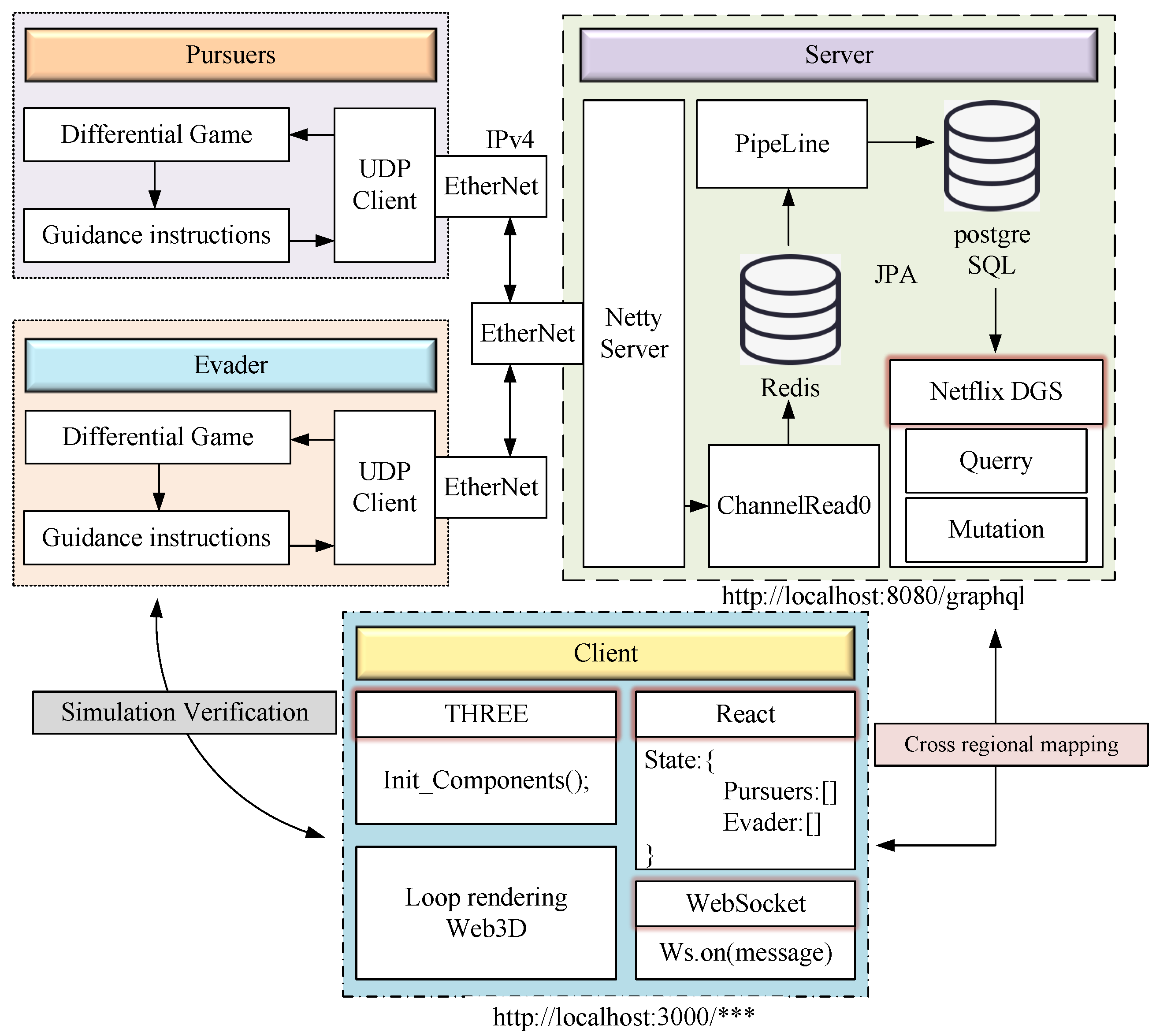
The simulation platform consists of three parts: the embedded hardware section, the backend built using a server, and the frontend presented by the browser. The overall framework design is shown in Figure 8.

In the embedded hardware, we used the Nvidia-developed Jetson Nano development board as the pursuer in the differential game, and the Raspberry Pi as the evader in the differential game. These two embedded development boards are connected to a switch via Ethernet ports, and the switch is connected to the local server. The backend server uses the Java programming language with the Spring Boot framework, which internally supports the Tomcat server. The asynchronous communication framework is Netty. The data from the underlying hardware is sent to the backend server via UDP communication. The embedded hardware in the second part makes the already small memory even more limited. In terms of database management, we use Redis as a caching database, which caches and updates data via pipeline stream technology. Additionally, we use PostgreSQL as the relational storage database to store the data of both parties in the game. This pipeline stream technology and asynchronous framework help prevent data packetization issues.

For the frontend, we use React, with Netflix DGS providing methods for querying and modifying data. The DGS framework’s main feature is its annotation-based Spring Boot programming model, which has lower server overhead compared to traditional Restful APIs. GraphQL is mainly used for temporary queries and operations. Queries are used to fetch data and return the found data, while mutations are used to modify data. The entire technology stack is based on a B/S structure, with communication conducted through HTTP protocols. The application includes methods for processing data and mapping the data of the pursuers and evaders. Three-dimensional modeling uses Three.js and Cesium.js.

Firstly, the pursuers and the evader upload their positions and attitude angles to the server through UDP communication. Once the server receives the data, it calls the asynchronous program ‘Channelread0’ to write the data into the Redis cache database and uses pipeline stream technology to update the data in real-time to the PostgreSQL database. Netty sends messages between them. After receiving each other’s information, the pursuers and the evader calculate the optimal strategy through differential game theory, give guidance commands, and calculate the next moment’s position and attitude through the motion model, then update the data again. Since UDP communication can sometimes lose data, no multithreading solution is used to ensure real-time data reception.

On the frontend, the page rendering is completed when the application is launched. When the server writes data for the PostgreSQL database and updates it, a long connection between the frontend and backend is triggered, and the updated data are sent through Mutation. After receiving the updated information, the frontend uses a data mapping scheme to write the updated data into the state. At the same time, the position and attitude of the pursuers and evaders are updated in real-time. Both the Jetson Nano and Raspberry Pi development boards support the Python 3.9 compiler. The paper attempts to use hardware development boards with identical configurations.

The Q-learning algorithm is trained offline using a simulated environment where the pursuers learn to intercept the evaders based on various escape patterns. The offline training phase allows for computationally intensive processes, such as model optimization and fine-tuning, to be performed without the constraints of real-time processing. After training, the model is deployed on an embedded platform, such as Jetson Nano or Raspberry Pi, for online use, where it guides the pursuers in real-time interception. By separating the training and execution phases, our approach reduces the computational load during real-time operations. This allows the system to run on less powerful embedded hardware, such as the Jetson Nano or Raspberry Pi, while still benefiting from the rich training data and complex computations performed offline.

This paper validates the feasibility of the proposed algorithm through the simulation platform. To simulate this process more accurately, the observation coordinate system is projected onto the geocentric coordinate system for analysis. Hardware parameters are shown in

Table 2. Hardware parameters.

Item	JetNano	Raspberry Pi
CPU	ARM CORTEX-A57	ARM CORTEX-A72
Storage	16 GB EMMC 5.1	16 GB EMMC 5.1
Memory	4 GB	4 GB
Network	Gigabit Ethernet	Gigabit Ethernet

. The data transmission protocol is shown in Figure 9.

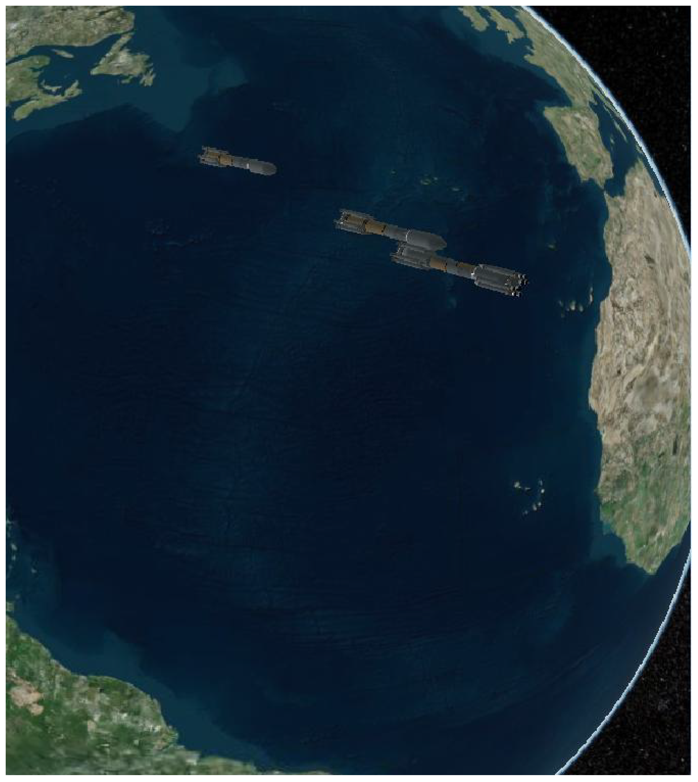
Figure 10 shows the 3D visualization effect of the system, clearly presenting the interaction and interception process between the pursuer and the evader. This page greatly enhances the user experience through vivid dynamic effects and interactive feedback, making the system’s state and behavior more intuitive and understandable.

Figure 11 presents the structure and functionality of the backend server, which is responsible for processing core data calculations and interactive operations, ensuring the stable operation of the system and supporting real-time communication with the frontend and the database.

Figure 12 and Figure 13 show real-time data from the database, reflecting the dynamic changes of the evader and the pursuer. These figures accurately reflect key data and real-time states during the entire pursuit process, providing detailed monitoring information.

7. Experimental Results

Next, this paper presents three different examples to demonstrate the interception process using the proposed Q-learning-cover algorithm.

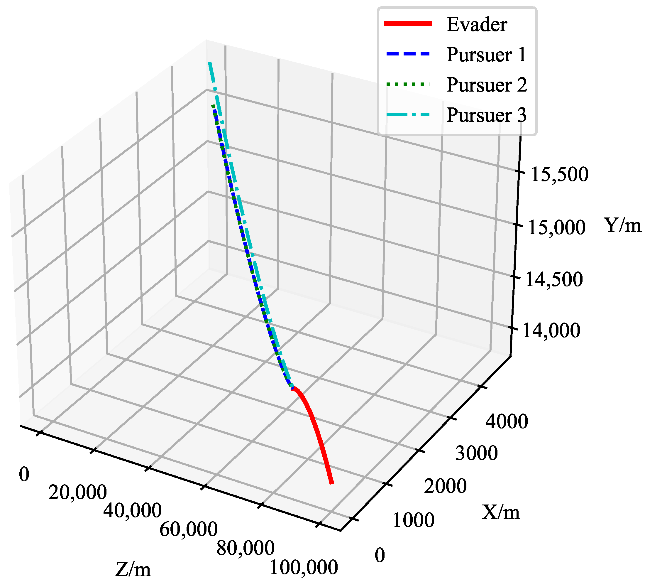
Example 1: The initial position of pursuer 1 is [0, 14,005, 4546], the initial position of pursuer 2 is [0, 15,892, 5025], and the initial position of pursuer 3 is [0, 14,543, 5072]. The pursuers’ speed is 4000 m/s. The initial position of the target is [100,000, 14,000, 0], and the target tries to evade the pursuers with a speed of 3000 m/s. The y- and z-coordinates of the pursuers’ initial positions are random. The initial distance between the pursuers and the evader is approximately 100,000 m, and the initial angle is random. The motion trajectories are shown in Figure 14.

Figure 14 shows the motion trajectories of the target and the pursuers in three-dimensional space. The red line represents the trajectory of the evader, while the blue, green, and cyan dashed lines represent the trajectories of the three pursuers. The figure demonstrates the relative position between the pursuers and the evader, as well as the distance variation between the target and the pursuers. Using the Q-learning-cover algorithm, the pursuers gradually reduce the distance to the target and ultimately capture it.

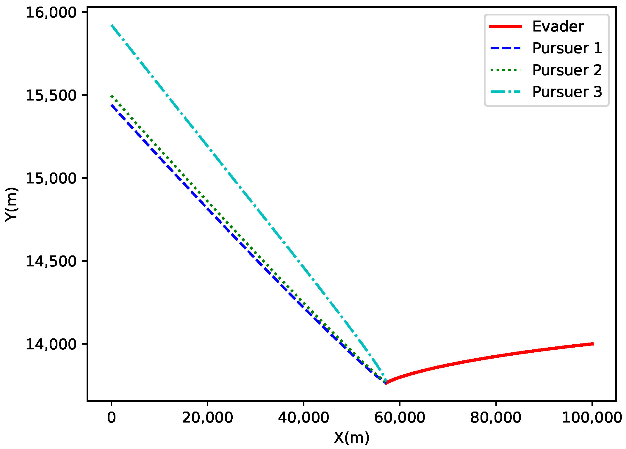
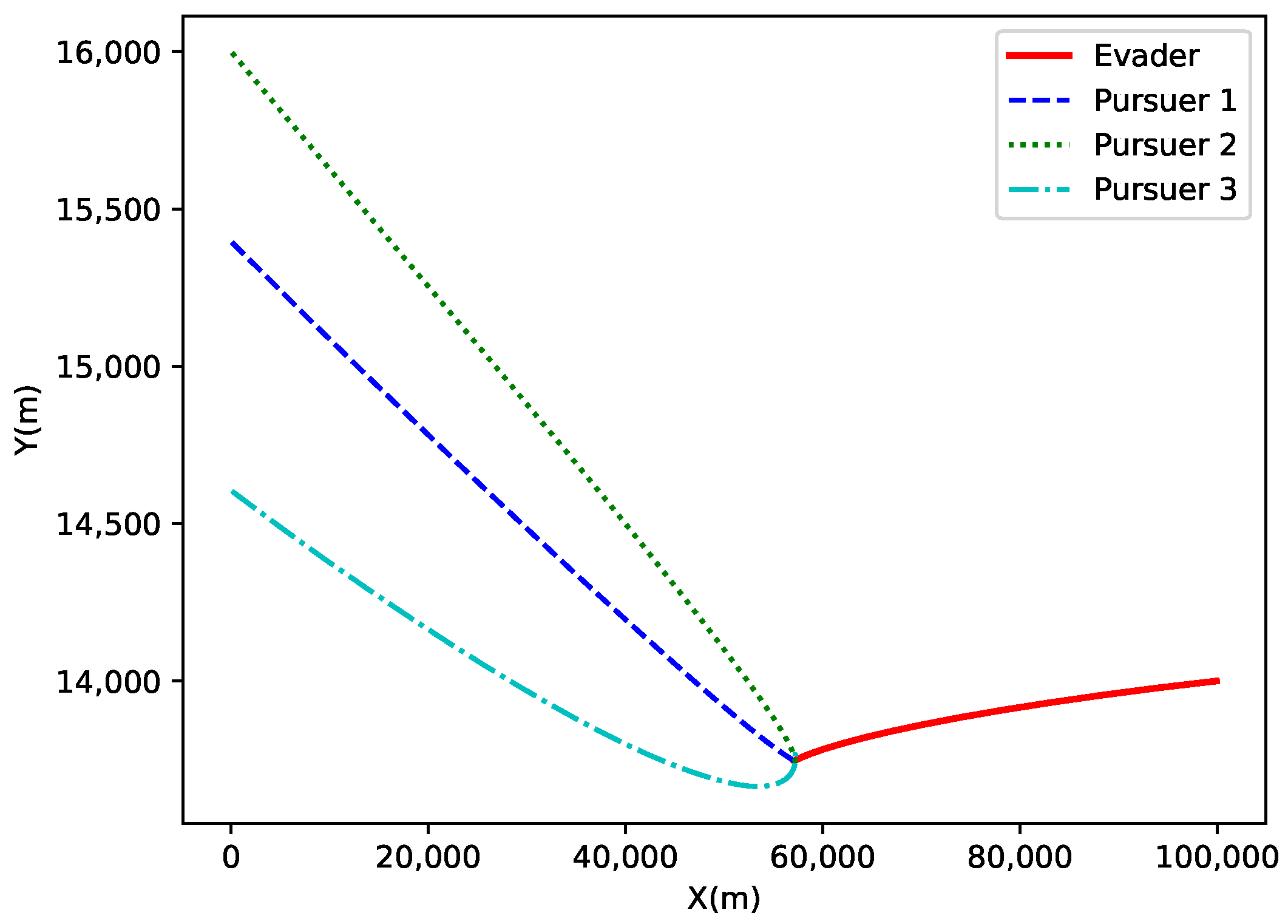
The X-Y axis projection is shown in Figure 15. This figure presents the projection of the target and the three pursuers on the X-Y plane. The trajectories of the evader and the pursuers are distinct in the X-Y plane due to their different initial positions. The evader’s trajectory shows a rapid offset, while the pursuers’ trajectories gradually converge towards the target based on their initial positions and motion directions.

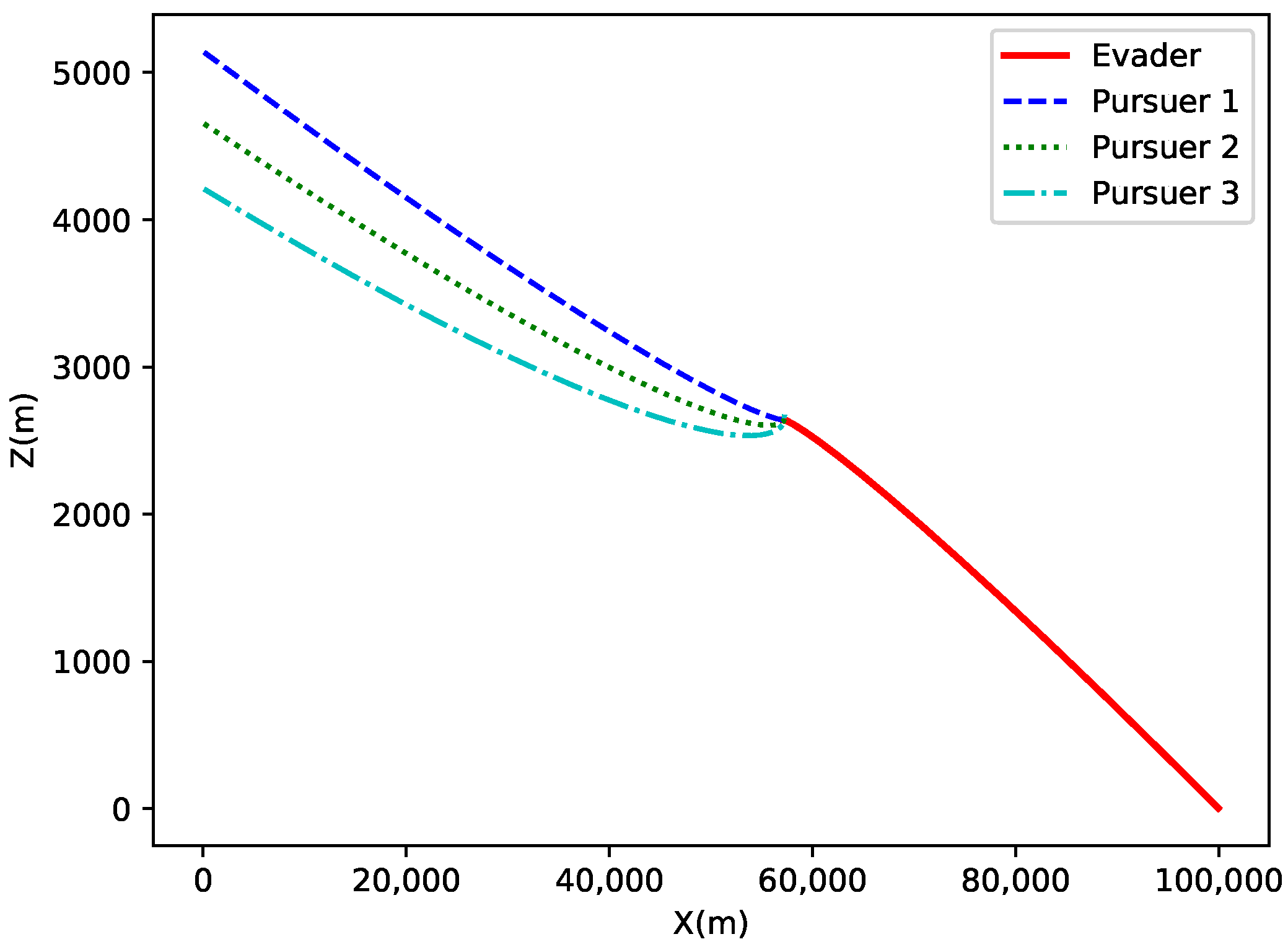
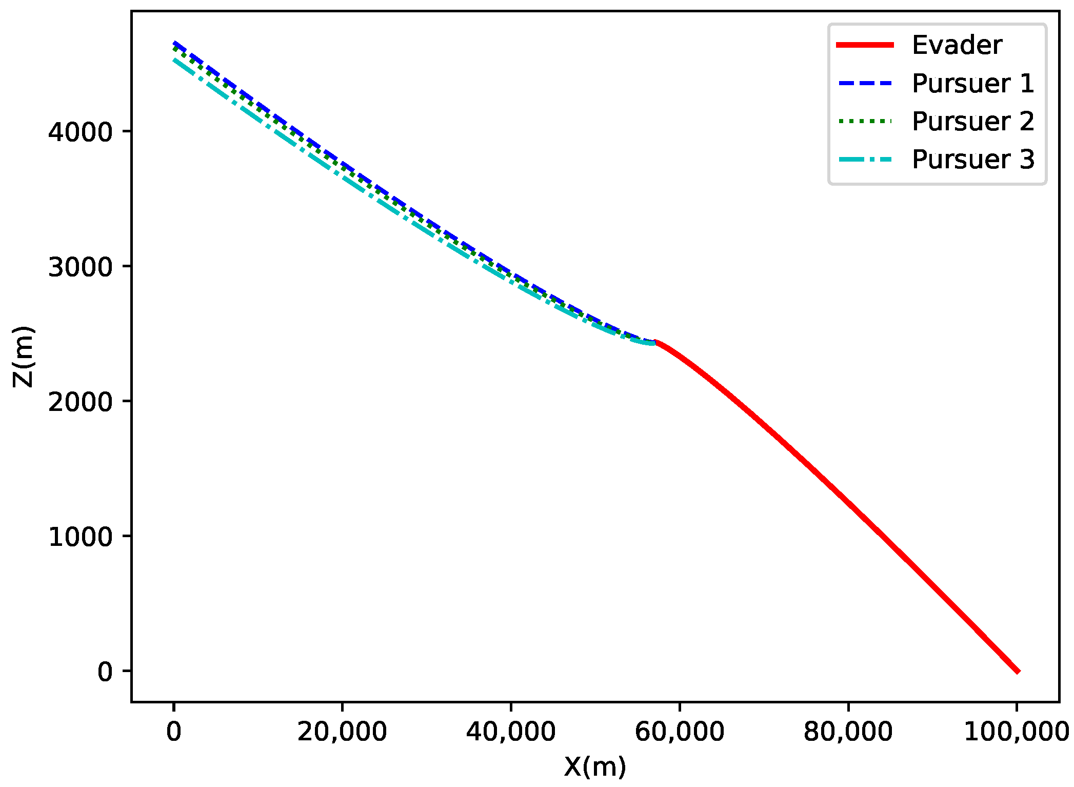
The X-Z axis projection is shown in Figure 16. This figure presents the projection of the target and the three pursuers on the X-Z plane. The evader’s trajectory shows a rapid displacement along the X-axis, while the pursuers’ trajectories gradually approach the target, demonstrating the motion characteristics of different pursuers and the effectiveness of the algorithm.

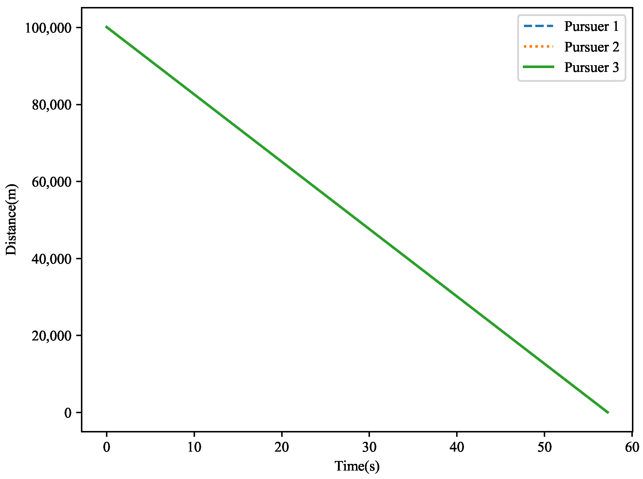
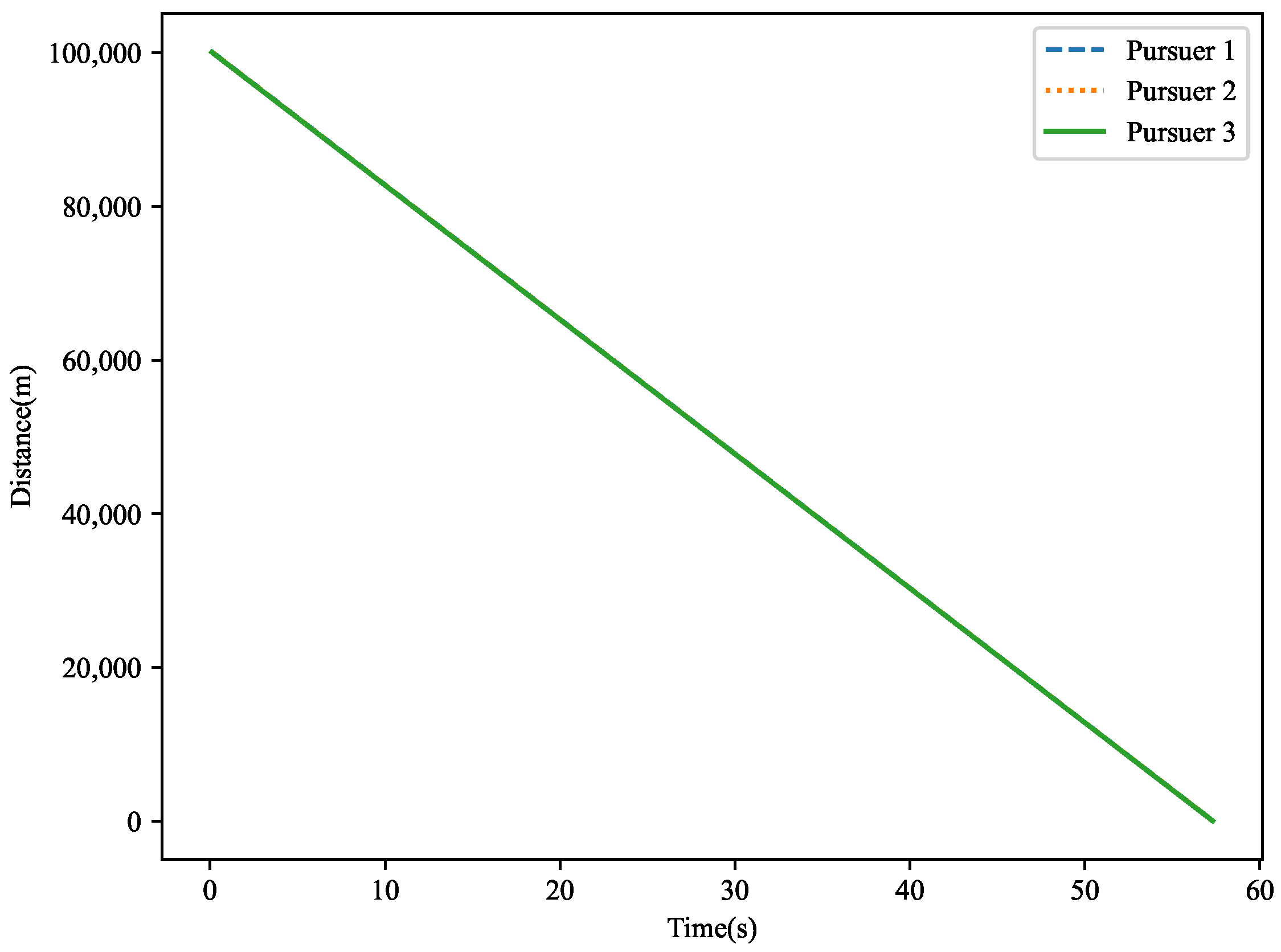
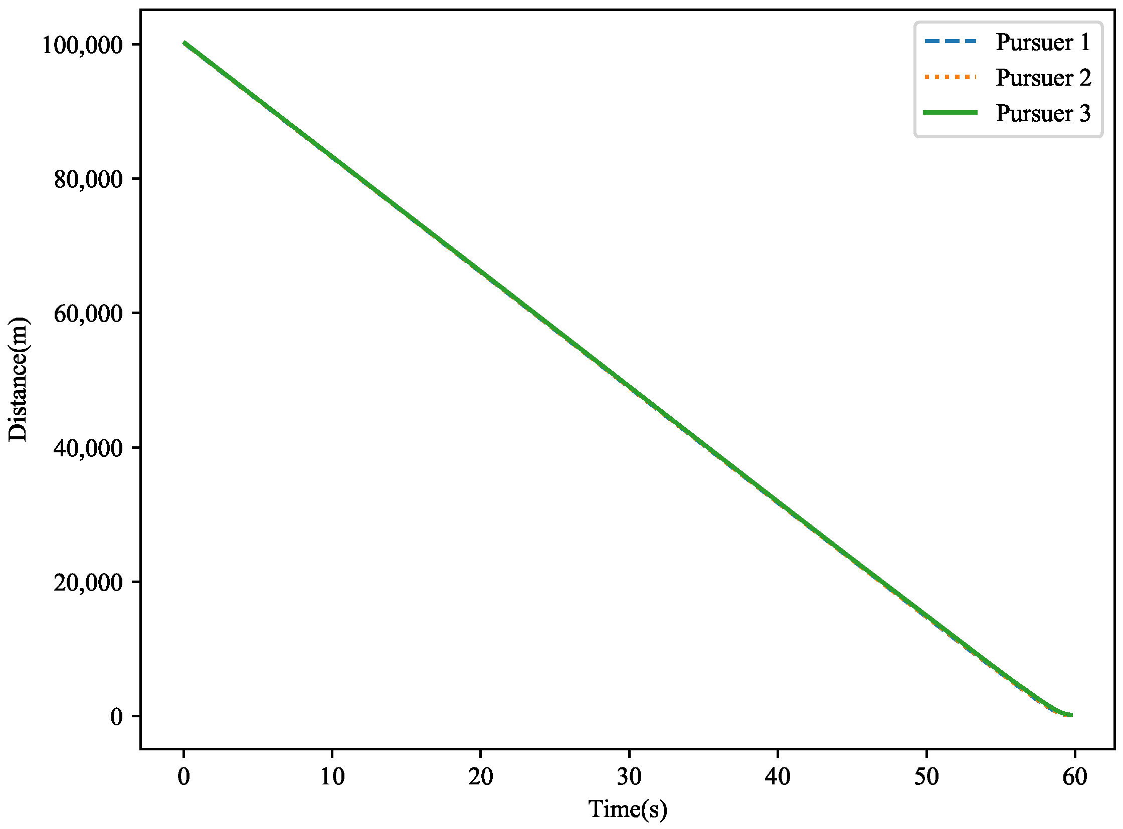
The distance variation is shown in Figure 17. This figure illustrates the distance changes between the target and the three pursuers in three-dimensional space. Over time, the target is gradually approached by the pursuers. Ultimately, the miss distances are $1.2\mathrm{m}$, $0.9\mathrm{m}$, and $1.5\mathrm{m}$, with the target being successfully captured by pursuer 2.

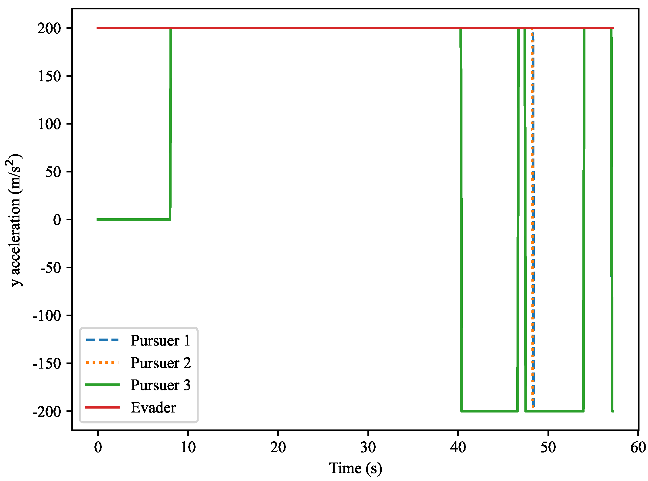
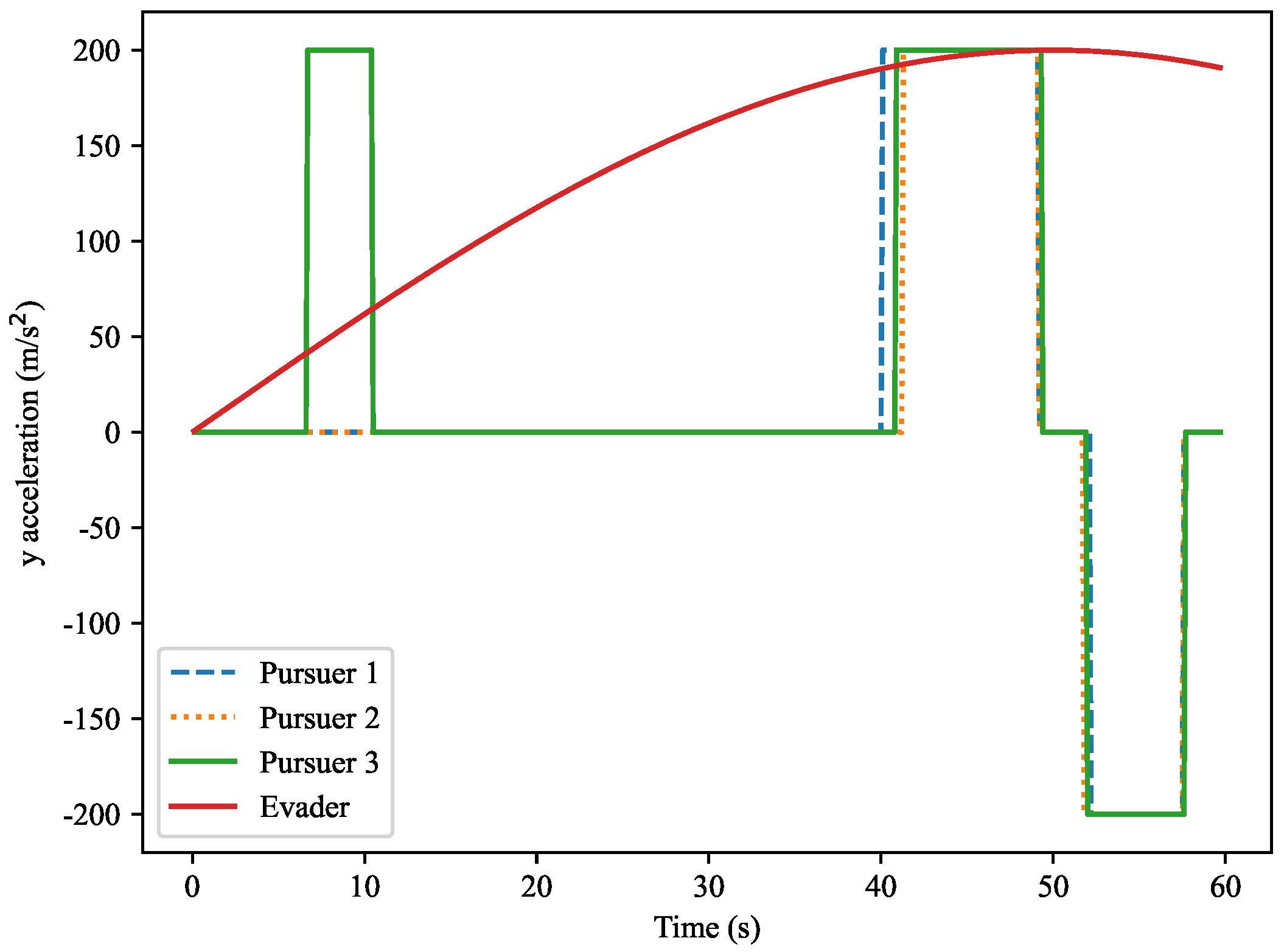
The Y-axis normal acceleration variation is shown in Figure 18. This figure presents the variation in normal accelerations along the Y-axis for the evader and the three pursuers. Over time, the accelerations of the pursuers fluctuate significantly, especially during the capture process. The evader’s acceleration remains relatively stable, close to zero. The curves in the figure show the acceleration changes required by each pursuer based on their current motion trajectory.

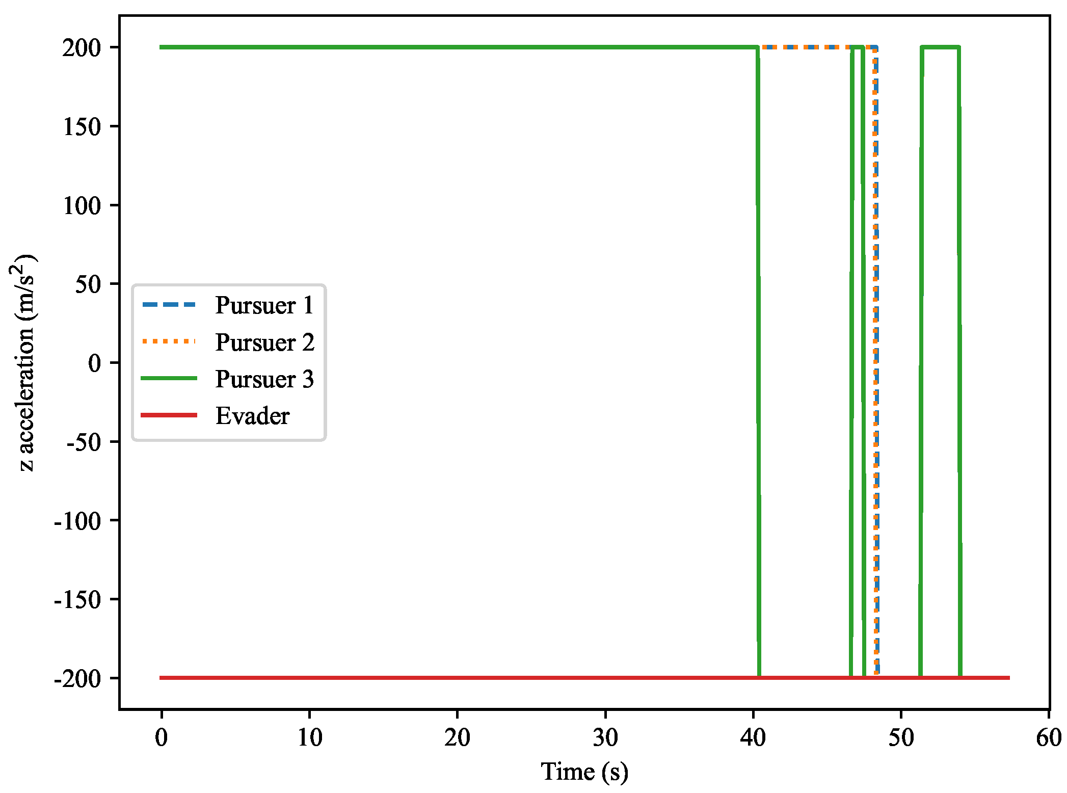
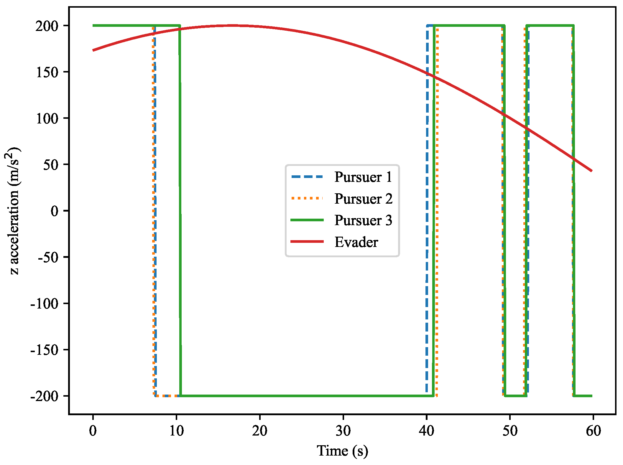
The Z-axis normal acceleration variation is shown in Figure 19. This figure shows the normal acceleration along the Z-axis for both the target and the pursuers. Similarly to the Y-axis acceleration, the pursuers’ accelerations exhibit significant fluctuations during the capture process, while the evader’s acceleration remains relatively small and close to zero. The figure shows that as the distance between the pursuers and the target changes, the fluctuations in acceleration become more pronounced.

Example 2: The maximum normal acceleration of the pursuers and the evader is set to 40 g, while other conditions remain the same as in Example 1. The initial position of pursuer 1 is [0, 14,399, 5250], the initial position of pursuer 2 is [0, 15,481, 4543], and the initial position of pursuer 3 is [0, 14,324, 5211]. The target’s initial position is [100,000, 14,000, 0], and the maximum normal acceleration is set to 40 g, which means that the pursuers’ acceleration is restricted to a higher value, thus affecting their efficiency and strategy in capturing the target.

The motion trajectory is shown in Figure 20. The figure displays the motion trajectories of the evader and the three pursuers in three-dimensional space. The trajectories of the pursuers and the evader differ from those in Example 1, especially after the change in the acceleration limit. The pursuers’ trajectories show more significant changes. Through the Q-learning-cover algorithm, the pursuers gradually approach the target and ultimately capture it.

The X-Y plane projection is shown in Figure 21. This figure presents the projection of the target and the three pursuers on the X-Y plane. Compared to Example 1, the motion trajectories of the pursuers and the evader exhibit different changes in this plane. Particularly, with the normal acceleration limit set to 40 g, the pursuers’ movement becomes more intense, and the trajectory changes are more pronounced. The evader maintains a relatively stable path in the X-Y plane, while the pursuers’ trajectories show their continuous approach toward the target. By comparing the trajectories of the pursuers, the dynamic changes during the pursuit process are clearly observed.

The X-Z plane projection is shown in Figure 22. This figure presents the projection of the target and the three pursuers on the X-Z plane. With the normal acceleration limit set to 40 g, the pursuers’ trajectories show more complex dynamic changes on this plane, especially during the capture process. The pursuers’ paths exhibit larger fluctuations, while the evader’s trajectory remains more stable, despite the pursuers closing in. Comparing the projections of the pursuers in the X-Z plane helps in understanding the impact of acceleration on the pursuers’ movement paths.

The distance variation is shown in Figure 23. This figure displays the distance variations between the evader and the three pursuers. As the pursuers gradually approach the target, the final miss distances are $6.3\mathrm{m}$, $0.7\mathrm{m}$, and $2.2\mathrm{m}$. The curves in the figure show the dynamic changes during the pursuit. In this example, due to the normal acceleration being set to 40 g, the pursuers’ acceleration is significantly increased, leading to more dramatic trajectory changes during the capture process. By comparing the distance variation curves of the pursuers, one can clearly see the acceleration and deceleration processes at different stages of the pursuit.

The Y-axis acceleration variation is shown in Figure 24. This figure presents the variation in acceleration along the Y-axis for the evader and the three pursuers. In this example, the acceleration of the pursuers fluctuates significantly, especially as they approach the target. As their acceleration increases, the pursuers’ trajectories gradually close in on the target. In contrast, the evader’s acceleration remains relatively stable, staying at a low level. By comparing the acceleration variations of the pursuers and the evader, the effect of acceleration on the pursuit strategy is clearly observable.

Z-axis acceleration variation is shown in Figure 25. This figure presents the variation in acceleration along the Z-axis for the target and the pursuers. Similar to the Y-axis acceleration, the pursuers’ acceleration fluctuates more significantly as they approach the target, showing obvious variations. The evader’s acceleration remains relatively stable, with consistent values. By comparing the acceleration differences between the pursuers and the evader, the impact of acceleration on the capture process is intuitively observed.

Experiment 3: The pursuers use the optimal strategy, and the evader uses a composite sine maneuver. Other conditions are the same as in Example 1. The initial position of pursuer 1 is [0, 14,399, 5250], the initial position of pursuer 2 is [0, 15,481, 4543], and the initial position of pursuer 3 is [0, 14,324, 5211]. The initial position of the target is [100,000, 14,000, 0]. Unlike the previous two examples, the evader in this example adopts a composite sine maneuver strategy, making its trajectory more complex and unpredictable, thereby increasing the difficulty for the pursuers to capture the target. The 3D trajectory is shown in Figure 26.

The initial distance between the pursuers and the evader is approximately 100,000 m. The initial angle is random. The figure displays the motion trajectories of the evader and the three pursuers in three-dimensional space. Due to the composite sine maneuver of the evader, the trajectory shows more complex and variable characteristics. With the optimal strategy, the pursuers gradually close the distance to the target and eventually capture it.

X-Y plane projection is shown in Figure 27. This figure presents the motion trajectories of the evader and the three pursuers in the X-Y plane. Compared to Example 1, the motion trajectories of the pursuers and the evader exhibit different changes in this plane. Particularly, with the normal acceleration limit set to 40 g, the pursuers’ movement becomes more intense, and the trajectory changes are more pronounced. The evader maintains a relatively stable path in the X-Y plane, while the pursuers’ trajectories show their continuous approach toward the target. By comparing the trajectories of the pursuers, the dynamic changes during the pursuit process are clearly observed.

The X-Z plane projection is shown in Figure 28. This figure presents the motion trajectories of the evader and the three pursuers in the X-Z plane. With the normal acceleration limit set to 40 g, the pursuers’ trajectories show more complex dynamic changes on this plane, especially during the capture process. The pursuers’ paths exhibit larger fluctuations, while the evader’s trajectory remains more stable, despite the pursuers closing in. Comparing the projections of the pursuers in the X-Z plane helps in understanding the impact of acceleration on the pursuers’ movement paths.

The distance variation is shown in Figure 29. This figure displays the distance variations between the evader and the three pursuers over time. As the pursuers gradually approach the target, the final miss distances are 3.6 m (pursuer 1), 0.92 m (pursuer 2), and 2.3 m (pursuer 3). The curves in the figure display the dynamic changes during the pursuit. In this example, with the normal acceleration being set to 40 g, the pursuers’ acceleration is significantly increased, leading to more dramatic trajectory changes during the capture process. By comparing the distance variation curves of the pursuers, one can clearly see the acceleration and deceleration processes at different stages of the pursuit.

The Y-axis acceleration variation is shown in Figure 30. This figure presents the variation in acceleration along the Y-axis for the evader and the three pursuers during the pursuit. The evader’s Y-axis acceleration curve (red solid line) shows an overall increasing trend, which then stabilizes, reflecting the sustained control signals applied during its evasion or turning maneuvers. The pursuers’ acceleration curves exhibit significant jumps, especially for pursuer 3 (green dashed line), where acceleration spikes are observed during multiple periods, likely due to its rapid path correction behavior. Pursuers 1 and 2 show relatively smoother acceleration curves, indicating stable control strategies, contributing to higher precision tracking.

The Z-axis acceleration variation is shown in Figure 31. The figure shows the acceleration variations along the Z-axis for both the target and the pursuers. Similar to the Y-axis acceleration, the pursuers’ acceleration fluctuates more significantly as they approach the target, with obvious spikes in their acceleration. The evader’s acceleration remains relatively steady, with consistent values. Comparing the acceleration differences between the pursuers and the evader provides a more intuitive understanding of how acceleration differences impact the capture process.

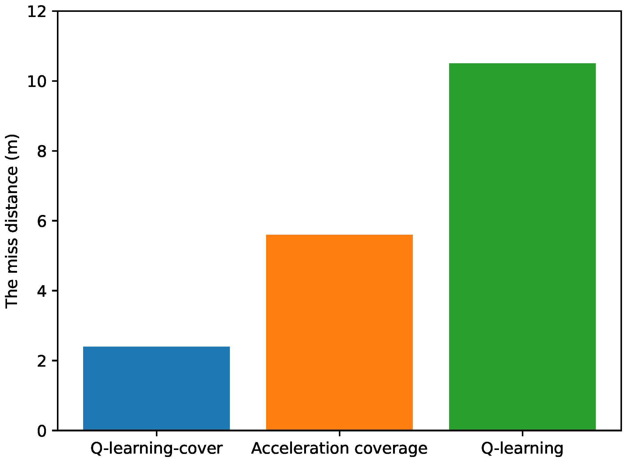
Comparison of three algorithms: This paper compares the Q-learning-cover algorithm with the acceleration coverage algorithm in terms of miss distance. The experiment was repeated 100 times, and the average miss distance for the three pursuers was calculated, as shown in Figure 32. The experimental results show that the Q-learning-cover algorithm’s average miss distance is 2.4 m, the acceleration coverage algorithm’s average miss distance is 5.8 m, and the Q-learning algorithm’s miss distance is 10.4 m. This demonstrates that the Q-learning-cover algorithm has a clear advantage in improving interception accuracy.

In Figure 33, we present an analysis of the experimental results. The left side of the figure shows the process of three pursuers successfully intercepting one evader, while the right side presents the real-time feedback of the browser monitoring data. Unlike the experimental setup in Section 2, this experiment was conducted in the Earth coordinate system and used advanced Cesium technology for visualization, achieving more precise and dynamic monitoring displays.

Tabular comparison of existing approaches: As per the recommendation, we have included a tabular comparison (

Table 3. Average comparison results of 100 experiments.

Method	Interception Success Rate (%)	Convergence Time (s)	Memory Requirement (MB)
Q-learning-cover	97	0.002	54
PN	87	0.003	82
ZCMD	92	0.004	120
DDPG	89	0.021	96

) between existing methods (PN, ZCMD, and DDPG) and the Q-learning-cover algorithm. This comparison presents the results based on accuracy, convergence time, and computational complexity, providing a clearer perspective on how our method compares to others in the field. Table 3 presents a comparison of the Q-learning-cover algorithm with other existing methods, namely PN, ZCMD, and DDPG, based on three key metrics: interception success rate, convergence time, and memory requirement.

• Interception success rate: The Q-learning-cover algorithm achieved the highest interception success rate at 97%, significantly outperforming the other methods, with PN at 87%, ZCMD at 92%, and DDPG at 89%. This indicates that the Q-learning-cover algorithm excels in accuracy, making it a highly effective approach for strategic interception.
• Convergence time: The Q-learning-cover algorithm also demonstrated the shortest convergence time (0.002 s), suggesting that it is computationally efficient compared to the other methods. In contrast, DDPG took the longest (0.021 s), followed by ZCMD (0.004 s) and PN (0.003 s).
• Memory requirement: Regarding memory usage, the Q-learning-cover algorithm required 54 MB, which is the least among all methods. This efficiency is critical for real-time applications, especially when hardware resources are constrained. DDPG required 96 MB, ZCMD 120 MB, and PN 82 MB.

Overall, these results show that the Q-learning-cover algorithm offers a promising balance between high interception accuracy, fast convergence, and low memory usage, making it an attractive option for real-world applications in pursuit–evasion scenarios.

The parameter $\alpha$ plays a crucial role in adjusting the proportional coefficients of the algorithm. As $\alpha$ increases, the accuracy of the interception improves, but this comes at the cost of increased computation time. We observe that larger values of $\alpha$ result in slower convergence times, suggesting a trade-off between accuracy and efficiency.

The parameter $\gamma$, which is related to the discount factor in the reinforcement learning setup, influences the weight given to future rewards. Increasing $\gamma$ leads to better long-term planning but may cause slower adaptation in dynamic environments. In our experiments, we found that varying $\gamma$ significantly affects the algorithm’s convergence speed.

Finally, the parameter $\lambda$ is crucial for scaling the velocity difference between the pursuer and evader. As $\lambda$ increases, the algorithm’s memory usage decreases, but at the cost of reduced accuracy in interception. The relationship between $\lambda$ and efficiency highlights a balance between resource consumption and interception precision.

In addition to the performance metrics presented in Table 3, we further analyze the algorithm’s efficiency by evaluating the computation time and the number of iterations required for convergence.

Computation time: The computation time is measured for each iteration of the algorithm, and we observe that the Q-learning-cover algorithm outperforms other methods in terms of speed, as shown in

Table 4. Computation time and number of iterations for 100 experiments.

Method	Computation Time (s)	Number of Iterations
Q-learning-cover	225	120
PN	346	150
ZCMD	443	180
DDPG	276	250

.

Number of iterations: The number of iterations required for the algorithm to reach convergence is also reported. We found that the Q-learning-cover algorithm requires fewer iterations compared to the other methods, which contributes to its faster convergence time.

The results show that the Q-learning-cover algorithm is both computationally efficient and fast in converging to the optimal solution with fewer iterations compared to other algorithms.

8. Conclusions

This paper presents a Q-learning-cover-based three-on-one pursuit interception algorithm that integrates Ahlswede sphere geometry and reinforcement learning. By projecting the 3D trajectories of pursuers and the evader onto the complex plane, the method significantly reduces computational complexity while maintaining high efficiency in planning the pursuers’ trajectories.

The algorithm’s boundedness is proven using a Lyapunov function, ensuring fast convergence and stability. The simulation results demonstrate that the Q-learning-cover algorithm improves pursuit efficiency and interception accuracy. The method shows promise for multi-agent systems such as drone swarms and robotic clusters, where it enhances the success rate and accuracy of pursuit tasks.

Future research will further investigate the extension of the Q-learning-cover algorithm to more complex pursuit scenarios, such as incorporating dynamic obstacles and multi-evader situations. For instance, the algorithm could be adapted to handle real-time avoidance and interception strategies for both moving obstacles and multiple evaders, which would be essential for applications like autonomous vehicles and multi-robot coordination. The development of more advanced models, such as model predictive control (MPC)-based methods and deep reinforcement learning algorithms, could also enhance the algorithm’s ability to manage non-linear dynamics and long-term planning.