Research on Surrogate Model of Variable Geometry Turbine Performance Based on Backpropagation Neural Network

Abstract

To meet the increasingly stringent performance indicators of gas turbines, the turbine inlet temperature has increased, and variable geometry turbine technology is widely applied. Therefore, this study developed a quasi-two-dimensional (quasi-2D) method for variable geometry turbine performance considering cooling air mixing based on the elementary blade method and the cooling airflow mixing model. To address the high-dimensional, multi-variable data fitting problem of variable geometry turbines considering the effects of cooling air, this study adopted a BP neural network to further establish a surrogate model for variable geometry turbine performance. A sensitivity analysis of a single-stage turbine was conducted. The variable geometry cooling performance of a single-stage turbine and an E³ five-stage low-pressure air turbine were calculated, and the corresponding surrogate models were established. The relative errors between the calculated mass flow rate and efficiency of the single-stage turbine and the experimental values were no more than 0.70% and 4.44%, respectively; for the five-stage air turbine, the maximum relative errors in mass flow rate and efficiency were no more than 1.67% and 1.385%, respectively. When the throat area of the single-stage turbine nozzle changed by ±30%, the maximum relative errors between the calculated mass flow rate and efficiency and their experimental values were 3.602% and 4.228%, respectively; thus, the determination coefficients of the constructed BP neural network model for the training samples were all greater than 0.999, indicating that the surrogate model has high prediction accuracy and strong generalization ability and can quickly predict variable geometry turbine cooling performance.

1. Introduction

As key components of gas turbine engines, turbines can not only convert the energy of high-temperature gas into mechanical energy but also re-match the working point of components by adjusting the turbine nozzle area (Variable Area Nozzle, VAN), thereby modulating the operating state of gas turbines/aero-engines. For example, the WR-21 five-stage power turbine, the NovaLT16 two-stage power turbine, and the LM1600 two-stage power turbine have all successfully applied variable geometry turbine (VGT) technology to improve their power maneuverability. VGT technology has also been used in variable-cycle technology validation machines such as GE21, VCTFE731-2, HYPR90, and COPE.

Relevant research institutes have extensively studied VGT technology. The Lewis Research Center in the United States conducted an experimental study on the effect of turbine guide throat area variation on turbine performance by closing down the throat area of a single-stage turbine [1,2,3] and a two-stage turbine [4] to 70% and then opening them up to 130%. They found that both closing down and opening up the turbine guide area reduced turbine efficiency, but closing it down made the efficiency decrease more significantly. Kozak [5] numerically simulated a two-stage variable geometry turbine system for a modern internal combustion engine in which the effect of three different guide vane positions on the turbine’s performance was considered. The results showed that the VAN technology significantly improved the efficiency of turbocharger systems. Galindo [6] proposed a model that can be used to simulate variable geometry turbochargers and validated it by performing a CFD numerical simulation of static and pulsating flow in a variable geometry radial turbine. Razinsky [7] tested a variable geometry GT-225 automotive gas turbine with a turbine guide vane position set to design, open or closed. The results showed that when the turbine guide vane was closed, efficiency was lower than when it was open, but the effect on the mass flow rate was larger. Yao [8] proposed a variable geometry turbine guide vane adjustment scheme with adjustable suction surfaces and compared its use with adjusting the stagger angle of turbine guide vanes. The influence of adjusting the guide vanes on turbine performance was tested through experiments and CFD numerical simulations, and the results showed that performance was better under the new guide vane regulation scheme. Yue [9] conducted a CFD numerical simulation on the radial clearance leakage flow of a variable geometry turbine, showing that leakage flow decreases when the stagger angle is between ±5°. Niu [10] conducted an experimental study on a variable geometry turbine using five stagger angles to investigate the effect of adjusting the guide vane on turbine performance. The results showed that opening or closing the guide stagger angle increased the total pressure loss and decreased the turbine efficiency.

To meet gas turbine/aero-engine performance requirements, turbine inlet temperatures have continued to increase, and turbines need to be cooled for safe and reliable operation. When the effects of variable geometry and cooling on turbine performance are considered together, the mass flow rate and efficiency are not only related to the rotational speed and expansion ratio of the turbine but also to the amount of cooling air and nozzle angle adjustment. To solve the multivariate and high-dimensional data processing problems brought by a variable geometry turbine, the effect of cooling air for practical engineering applications needs to be considered. In this study, a surrogate model for variable geometry turbine performance considering the effects of cooling air mixing was established using a BP neural network. In recent years, this neural network model has performed well in solving high-dimensional data fitting problems for gas turbine/aero-engine components.

Orkisz et al. [11] used a bivariate function to fit compressor and turbine performance and compared the bivariate function model with experimental data. The results showed that using second- or third-order bivariate polynomials can fit the compressor and turbine performance better and with high accuracy, and their relative errors do not exceed 2.0%. Liu et al. [12] created a surrogate model for predicting compressor and turbine performance based on an artificial neural network, facilitating the overall performance prediction and fault diagnosis for gas turbines. Lazzaretto [13] established a zero-dimensional model of a single-shaft gas turbine engine based on a neural network model. The results showed that the neural network model fit the engine performance with high prediction accuracy, using only a few computational resources. Bartolini [14] extended the compressor performance map of micro-gas turbines based on an artificial neural network, which was then used to predict micro-gas turbine performance and pollutant emissions. References [15,16,17] focused on fitting compressor performance and performance prediction based on neural networks. Liu [18] developed a loss model for a helium turbine based on a neural network model to improve the accuracy of turbine performance prediction. Galindo [19] simulated the combustion rate of an engine during transient operation based on an artificial neural network and developed a one-dimensional (1D) simulation model for predicting combustion performance. References [20,21,22] investigated the application of neural networks to combustion chamber operating performance. Nikpey [23] developed a performance model of a micro-gas turbine using an artificial neural network based on the performance data of a modified Turbec T 100 gas turbine, which was then used for monitoring and fault diagnosis. References [24,25,26,27,28] investigated the application of neural networks to fault diagnosis and health monitoring of gas turbines.

However, most of the current research on variable geometry turbine performance has focused on single-stage or two-stage turbines, and there have been no reports on performance prediction methods for multi-stage variable geometry turbines. Moreover, the hotspots in the literature on the performance fitting of gas turbine components are mainly focused on compressor, combustion chamber, and gas circuit diagnoses. Only a few studies in the literature have reported using surrogate models to solve the high-dimensional and multivariate data fitting problems of variable geometry turbines considering the influence of cooling air. Therefore, this study developed a method for quickly predicting the performance of a multi-stage variable geometry turbine considering the influence of cooling air based on a BP neural network. We also developed a related computational program. The main contributions and innovations of this study are as follows:

• A quasi-2D turbine performance prediction method was combined with a flow loss model and a deviation angle model. A variable geometry model and a cooling model were introduced to develop a variable geometry turbine performance prediction method considering cooling air mixing.
• A surrogate model for variable geometry turbine performance considering the effects of cooling air mixing was established using a BP neural network, realizing rapid prediction of multi-stage variable geometry turbine cooling performance.

2. Methods and Models

2.1. Quasi-2D Method

The actual gas flow in a turbine is complex, three-dimensional, unsteady, compressible, and viscous. To reasonably simplify calculations, the quasi-2D performance calculation program developed in this study made the following assumptions. More detailed information can be found in Reference [29].

(1)

The gas flow is a perfect gas with constant specific heat, and the flow is steady and adiabatic.

(2)

There is no gas flow migration between the streamtube, which is divided at equal heights in the radial direction along the turbine passage.

(3)

In each streamtube, the gas aerodynamic parameters at the mean radius are taken as the average value of its gas aerodynamic parameters.

(4)

In each streamtube, the total temperature, total pressure, and axial velocity of the gas flow remain constant in the radial direction, while the static temperature, static pressure, and tangential velocity of the gas flow change in the form of free vortexes in the radial direction.

(5)

In each streamtube, the mass flow rate per unit area is determined by the aerodynamic parameters at its mean radius and remains constant with the radial position.

In each turbine stage, five calculation stations are set up, and the through-flow section is divided into five streamtubes, as shown in Figure 1. The aerodynamic parameters at each calculation station are calculated row-by-row using the 1D meanline method. At the beginning of the turbine performance calculation, the inlet total temperature (T_t0), total pressure (p_t0), and outlet static pressure (p_s1) at the mean radius of the first-stage stator blade center of the streamtube ③ are provided. For the five streamtubes between calculation stations 0 and 1, starting with the calculation of the outlet aerodynamic parameters and mass flow rate of streamtube ③, a simplified radial equilibrium equation is used to determine the outlet static pressure of adjacent streamtubes. The outlet aerodynamic parameters and mass flow rate of streamtubes ①, ②, ④ and ⑤ are calculated separately to determine the outlet aerodynamic parameters and total mass flow rate of the first-stage stator blade (station 1). Then, according to the continuity equation, the inlet aerodynamic parameters of each streamtube are calculated (station 0). Then, the flow loss (Y) and outlet flow angle (α) of each streamtube are calculated based on the Kacker and Okapuu (K-O) loss model [30] and the Ainley and Mathieson (A-M) [31] deviation angle model, i.e., the inlet and outlet aerodynamic parameters and the total mass flow rate of the stator blade are calculated, as shown in Figure 2. The rotor calculation is similar to that of the stator and will not be repeated.

Through the stage-by-stage solution strategy, the turbine performance parameters are determined. The outlet aerodynamic parameters of a certain-stage turbine are the inlet aerodynamic parameters of the next-stage turbine to complete the calculation of the multi-stage turbine performance, as shown in Figure 3. The specific calculation process can be found in the literature [29,32,33].

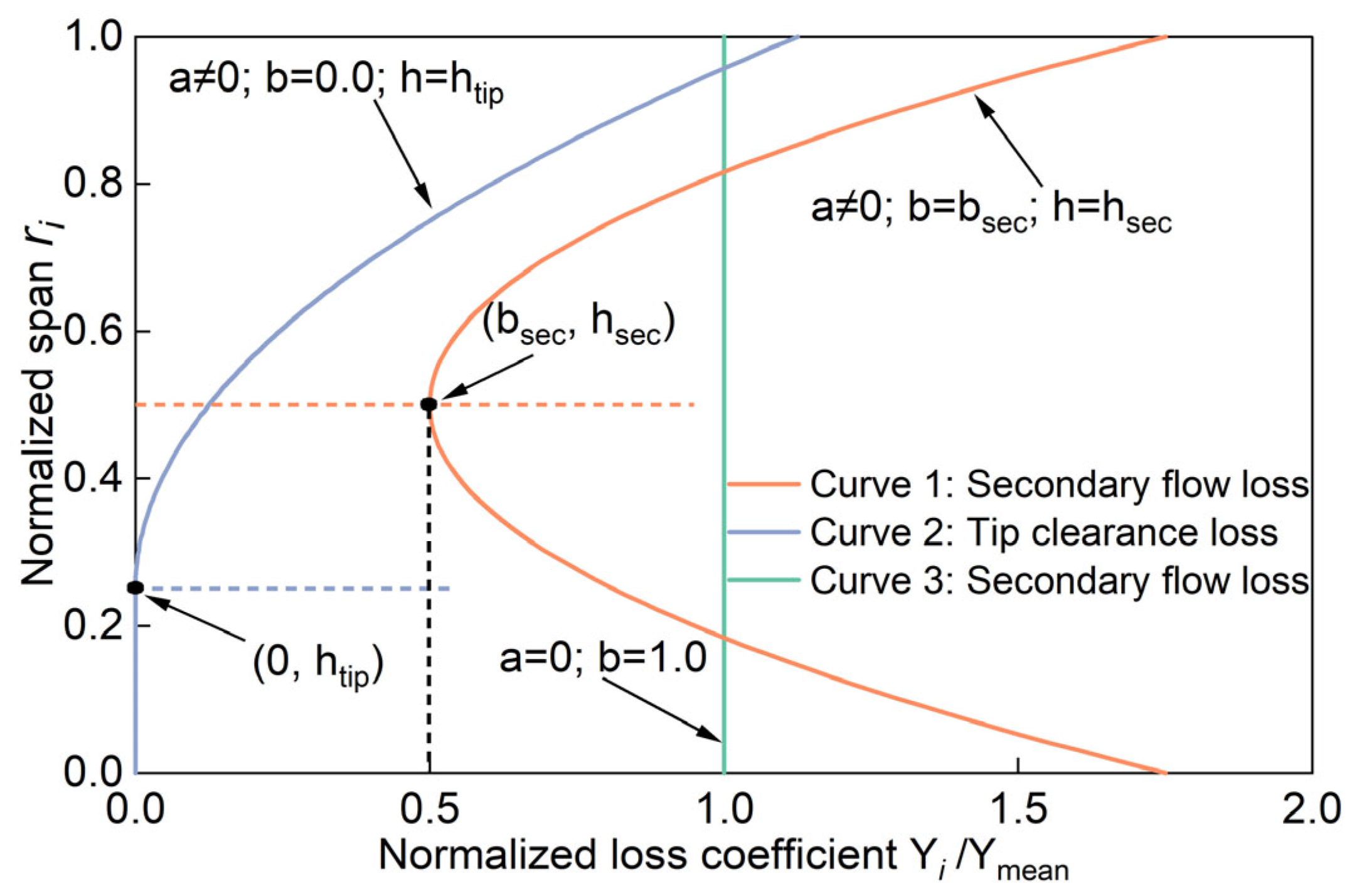
2.2. The Loss Distribution

In this study, the profile loss coefficient and trailing edge loss coefficient of each streamtube are directly calculated based on the profile geometric parameters and aerodynamic parameters at the mean radius of the local streamtube. Hosney et al. [34,35] demonstrated through experimental measurements that the secondary flow loss is greater in the end-wall region and relatively smaller at the mean radius (the mainstream region). Tip clearance loss is greater near the casing and relatively smaller at other locations. For these reasons, this study adopts a method similar to that in References [36,37] to deal with the radial distribution of secondary flow and tip clearance losses, that is, it is assumed that they follow a parabolic distribution pattern along the blade span.

$$Y_i/Y_{mean}=a{\left(r_i-h\right)}^2+b$$

(1)

In Equation (1), $a$, $h$, and $b$ are the three constants for determining the analytical formula of the parabola. $Y_i$ is the loss coefficient distributed to each streamtube. The parameter $r_i$ represents the normalized spanwise position from the hub to the mean radius of each streamtube, with its value ranging from 0 to 1. $Y_{mean}$ is the loss coefficient predicted by the K-O loss model, where the required profile geometric parameters and aerodynamic parameters are taken from the mean radius of the blade. $(b,h)$ is the vertex coordinate of the parabola. The form of the loss distribution can be conveniently regulated by changing the vertex coordinate, as shown in Curve 1 and Curve 2 in Figure 4. In particular, when $a=0$, Equation (1) degenerates into a linear function, that is, the secondary flow loss remains constant along the span direction. At this moment, $b=1.0$, as shown in Curve 3 in Figure 4. $h$ is the radial position of the blade height when the loss coefficient is at its minimum and $b$ is the normalized loss coefficient at the location of the minimum loss.

The constant $a$ in Equation (1) can be calculated by Equation (2).

$$Y_{mean}\times {\displaystyle \sum \begin{array}{l}{i}_{stre}\hfill \\ i=1\hfill \end{array}}{m}_i={\displaystyle \sum \begin{array}{c}{i}_{stre}\\ i=1\end{array}\left(Y_i\times m_i\right)}$$

(2)

where $i_{stre}$ is the number of streamtubes and $m_i$ is the mass flow rate in each streamtube.

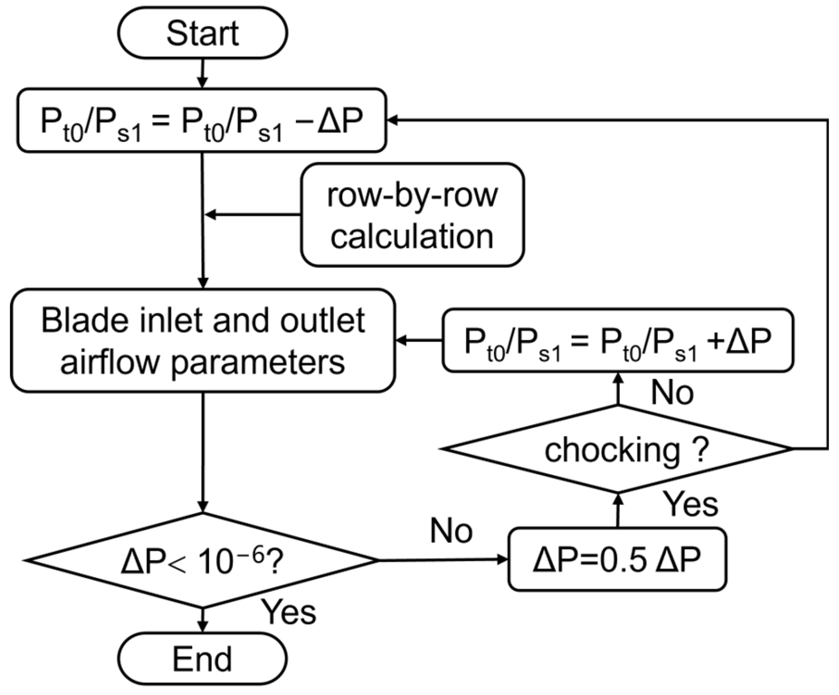
2.3. Determination of Turbine Choking Condition

The determination and calculation of turbine choking directly affect the accuracy of turbine performance prediction. This study takes the maximum flow capacity ($m_{\max }$) of the turbine blade row as the judgment basis for turbine choking. When the ratio of the nozzle inlet total pressure and outlet static pressure reaches the critical pressure ratio, the nozzle outlet section reaches the seed of sound and the nozzle flow capacity reaches its maximum. When the mass flow rate ($m_0$) flowing through a blade row of the turbine is greater than or equal to $m_{\max }$ of that blade row in a certain state, the turbine enters the choking state.

The turbine inlet mass flow rate is determined by giving the initial P_t0/P_s1 ratio of streamtube ③, which calculates the aerodynamic parameters in the cross-section of each calculation station in the turbine. When P_t0/P_s1 increases to a certain value, one of the blade rows in the turbine may be the first to appear in $m_0>m_{\max }$, and then, the choking iteration process begins to determine the choking mass flow rate and location of the turbine. The specific steps of the choking iteration for this blade row are shown in Figure 5.

When the pressure ratio increment (ΔP) is less than the pressure ratio tolerance limit (10⁻⁶), the iteration is terminated. At this point, P_t0/P_s1 is the choking pressure ratio, and the choking iteration calculation for the blade row is complete. As the P_t0/P_s1 of the center streamtube of the relevant blade row continues to increase, when the last blade row choking iteration of the turbine is completed and futher reaches the limit expansion state, the turbine performance calculation is completed.

2.4. Variable Geometry Turbine Considering Cooling Air Mixing

When the guide vane stagger angle is variable, the quasi-2D method described in Section 2.1 should be used to calculate variable geometry turbine performance. It is only necessary to establish the correlation between the turbine guide vane stagger angle, $\gamma$, and its geometric parameters, such as the inlet metal angle, ${\beta }_1$; the outlet metal angle, ${\beta }_2$; the throat width, $o$; and the axial chord.

To reliably rotate the turbine guide blade, the tip clearance of the adjustable guide vane is taken as 1.8% of the height. A schematic diagram of the stagger angle variation of the turbine guide vane is shown in Figure 6.

${\beta }_1$, ${\beta }_2$, and $\gamma$ change synchronously, which can be calculated using the following formula.

$${{\beta }_1}^{\prime }={\beta }_1+\Delta \gamma$$

(3)

$${{\beta }_2}^{\prime }={\beta }_2-\Delta \gamma$$

(4)

where ${{\beta }_1}^{\prime }$ and ${{\beta }_2}^{\prime }$, respectively, are the inlet and outlet metal angles of the stator blade after the turbine guide vane is rotated and $\Delta \gamma$ is the variation in $\gamma$. When the turbine guide vane is opened, the blade throat area increases, and $\Delta \gamma$ takes a positive value. Conversely, $\Delta \gamma$ takes a negative value.

As shown in Figure 6, $o$ changes with the variation in $\gamma$. In the actual calculation, the following approximation is made: a vertical line is drawn from the trailing edge of one blade to the suction surface of the adjacent blade, and the suction surface between the vertical foot and the adjacent blade trailing edge point is considered a straight line. The length of the vertical line is $o$, and its calculation formula is as follows.

$$o=t\times \cos ({{\beta }_2}^{\prime })$$

(5)

According to the geometric relationship, the axial chord of the blade can be calculated using the blade chord and stagger angle according to the following formula.

$$c_a=c\times \cos (\gamma +\Delta \gamma )$$

(6)

where $c_a$ is the axial chord length after $\gamma$ variation and $c$ is the chord length.

Cooling technology for turbines can significantly increase the inlet gas temperature, thereby improving the overall performance of the gas turbine. In this study, a one-dimensional constant-pressure mixing model for compressible air flow [38] is adopted and applied to the two airflow mixing processes in the cascade, respectively, to calculate the pressure loss coefficient caused by the film cooling of the cascade. The specific calculation process can be found in References [38,39]. During the calculation process, the introduction of cooling air is considered as follows. Since injecting coolant at the trailing edge can lead to significant losses [38], for the single-stage turbine case, the cooling airflow is injected into the mainstream at the leading edge of the blades. The angle between the cooling airflow and the mainstream direction is 35° [38,39]. The cooling airflow injected into the rotor and stator blade rows each accounts for half. In the stator blade row, the total pressure of the cooling airflow is taken as the local mainstream total pressure, and the total temperature of the cooling airflow is taken as half of the local mainstream total temperature. In the rotor blade row, the relative total pressure of the cooling airflow is taken as the local mainstream relative total pressure, and the relative total temperature of the cooling airflow is taken as half of the local mainstream relative total temperature. In the mixing layer, the mainstream mass flow rate accounts for 5% of the total. For the five-stage turbine case, the treatment method is mostly the same as that of the single-stage turbine case. The difference is that the cooling airflow is evenly distributed between the four blade rows in the first two stages.

The operating state of a variable geometry cooling turbine is determined by four parameters: the expansion ratio, ${\pi }_T$; the relative corrected rotational speed, ${\overline{n}}_{cor}$; $\Delta \gamma$; and the mass flow rate of the cooling airflow, $m_{cool}$. Conversely, the parameters that characterize the turbine performance are the corrected mass flow rate, $m_{cor}$($m_{cor}=(m\sqrt{T_{t0}/288.15})/(P_{t0}/101325)$), or mass flow rate, $m$, and efficiency, $\eta$. The corrected rotational speed and corrected mass flow rate have been converted to standard sea-level conditions for the single-stage turbine. The variable geometry turbine cooling performance can be expressed as a functional equation.

$$m_{cor} or m=f({\pi }_T,{\overline{n}}_{cor},\Delta \gamma ,m_{cool})$$

(7)

$$\eta =f({\pi }_T,{\overline{n}}_{cor},\Delta \gamma ,m_{cool})$$

(8)

where $T_{t0}$ and $P_{t0}$ are the total temperature and total pressure at the turbine inlet, respectively, and $m$ is the inlet mass flow rate. $n_{cor}$ ($n_{cor}=n/\sqrt{T_{t0}/288.15}$) is the corrected rotational speed.

2.5. BP Neural Network Model

BP neural networks have demonstrated excellent performance in function approximation and shown accurate interpolation and extrapolation prediction abilities for unknown data. Therefore, this study used a BP neural network to construct a surrogate model for variable geometry turbine performance, considering the effect of cooling air mixing.

2.5.1. Acquisition and Pre-Processing of Performance Data

A quasi-2D performance calculation program for variable geometry turbines considering cooling airflow mixing was developed and used to obtain the sample dataset to train the BP neural network. Firstly, the $map\min \max$ function was used to normalize the sample set data in the interval [−1, 1] to avoid model inaccuracy due to differences in the order of magnitude of variables. Then, the sample data were randomly divided into a training set, a cross-validation set, and a testing set according to a ratio of 60%:20%:20%. The training set was used to update the network weights and continuously improve accuracy. The validation and test sets were used to test the generalization ability of the model trained by the training set, that is, how well it matches the data not involved in the training.

2.5.2. BP Neural Network Structure

${\pi }_T$, ${\overline{n}}_{cor}$, $\Delta \gamma$, and $m_{cool}$ are the inputs of the network, and $m_{cor}$ or $m$,$\eta$ are the outputs of the network. Thus, the BP neural network is a four-input and two-output structure.

Theoretically, the multi-hidden layer structure and number of nodes have a better fitting effect on the mapping relationship of multivariate nonlinearity. However, considering the complexity of the network, the training time, and the “overfitting” problem, this study adopts a double hidden layer network structure for the single-stage turbine case. The number of neurons in each layer is traversed within a range of 5 to 20, and the variation in the root-mean-square error (RMSE) with the number of hidden layer nodes is shown in Figure 7.

As shown in Figure 7, when the number of neurons in the first hidden layer is taken as 18 and the number of neurons in the second hidden layer is taken as 13, the RMSE between the actual values of the cross-validation set samples and the predicted value of the neural network is minimized, and the performance is optimal. Therefore, the two-hidden-layer BP network structure is 4-[18-13]-2. Considering the similarity between the single-stage and multi-stage turbine performance curves, the same two-hidden-layer BP network structure is used for the five-stage turbine example.

Considering the highly nonlinear performance between the input and output parameters of the turbine, the Log-Sigmoid function is chosen as the transfer function of the hidden layer, and the purelin linear function is chosen as the activation function of the output layer. The training function, trainlm, of the Levenberg–Marquardt (L-M) variable gradient backpropagation algorithm is used to train the constructed neural network. The maximum number of iterations is set to 1000, the mean square error threshold is set to $1\times {10}^{-7}$, and the number of overfitting validation failures is set to 6.

2.5.3. Model Evaluation Indicators

The accuracy of the BP neural network model prediction results is evaluated using the coefficient of determination (R²), the root-mean-square error (RMSE), the mean absolute error (MAE), and the mean absolute percentage error (MAPE). Their definitions are as follows.

$$R^2=1-{\displaystyle \frac{{\displaystyle \sum \begin{array}{c}n\\ i=1\end{array}{(y_i-y_{pre,i})}^2}}{{\displaystyle \sum \begin{array}{c}n\\ i=1\end{array}{(y_i-{\overline{y}}_i)}^2}}}$$

(9)

$$RMSE=\sqrt{{\displaystyle \frac{1}{n}}{\displaystyle \sum \begin{array}{c}n\\ i=1\end{array}{(y_i-y_{pre,i})}^2}}$$

(10)

$$MAE={\displaystyle \frac{1}{n}}{\displaystyle \sum \begin{array}{c}n\\ i=1\end{array}\left|y_i-y_{pre,i}\right|}$$

(11)

$$MAPE={\displaystyle \frac{1}{n}}{\displaystyle \sum \begin{array}{c}n\\ i=1\end{array}\left|\frac{y_i-y_{pre,i}}{y_i}\right|}\times 100\%$$

(12)

where $y_i$ represents the actual value, $y_{pre,i}$ represents the model predicted value, and ${\overline{y}}_i$ represents the average of the actual values.

3. Results and Analysis

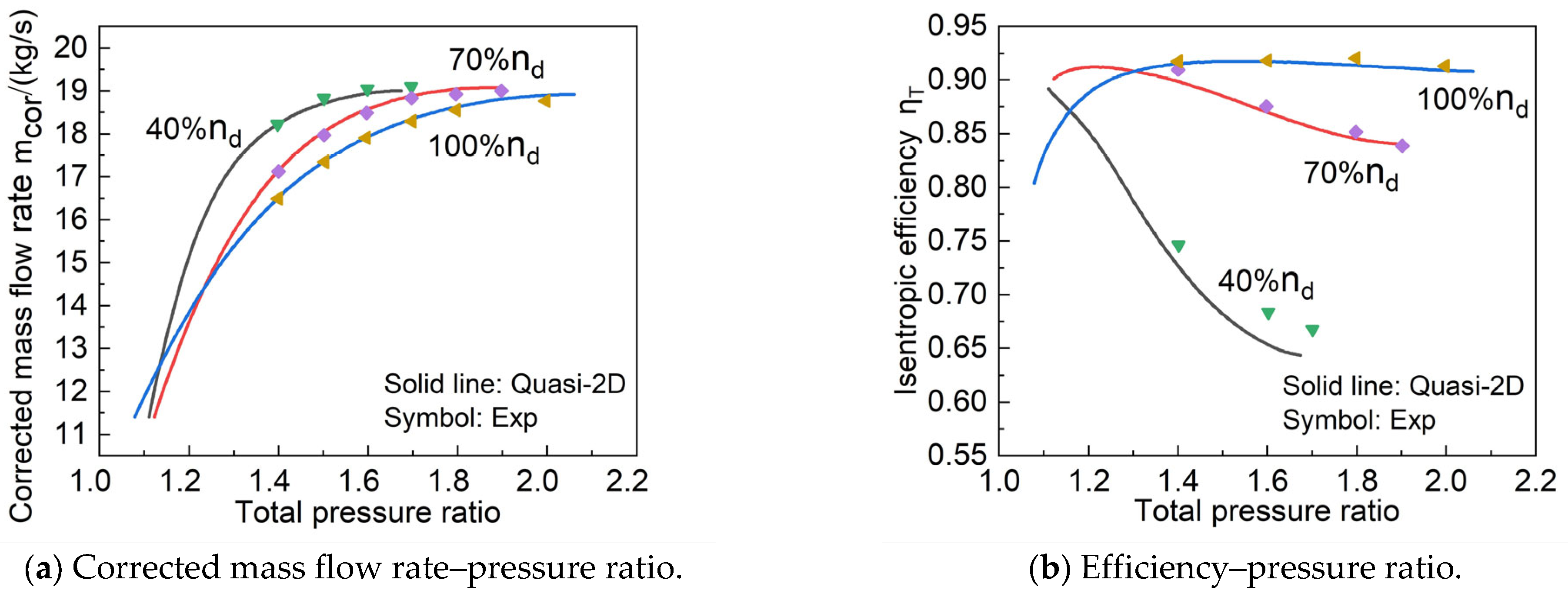
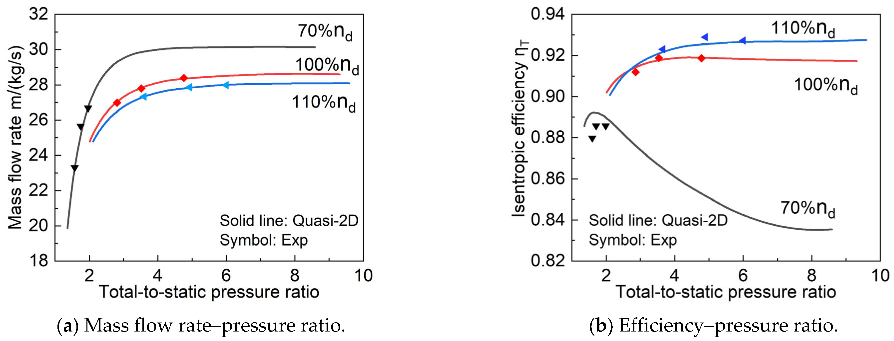
3.1. Validation of the Fixed Geometry Turbine

A NASA TN D-4389 single-stage turbine was selected to verify the accuracy and reliability of the quasi-2D method. The design parameters are shown in

Table 1. Single-stage turbine design parameters [40,41].

Design Parameters	Value
Design corrected rotational speed ($rpm$)	4407.4
Inlet total temperature ($K$)	299.8
Inlet total pressure ($Pa$)	101,590
Corrected mean blade speed $m/s$	152.40
Expansion ratio	1.798
Corrected mass flow rate, $m_{cor}$($kg/s$)	18.10

, and the geometric parameters are shown in

Table 2. Blade geometric performance [40,41].

Parameters	Value
Outer diameter, cm (inches)	76.2 (30)
Mean diameter, cm (inches)	66.04 (26)
Inner diameter, cm (inches)	55.88 (22)
Number of stator blades	50
Number of rotor blades	61
Blade length, cm (inches)	10.16 (4)
Radial tip clearance, cm (inches)	0.0762 (0.030)
Geometric performance at the mean radius	Rotor blade	Stator blade
Leading edge radius-to-chord ratio	0.065	0.066
Trailing edge radius-to-chord ratio	0.015	0.015
Maximum thickness-to-chord ratio	0.20	0.22
Chord, cm (inches)	5.82 (2.290)	5.18 (2.263)
Solidity	1.71	1.385
Aspect ratio	1.75	1.77

. Detailed geometric parameters and other parameters can be found in References [40,41]. For the single-stage turbine, both the corrected rotational speed and the corrected mass flow rate have been converted to standard sea-level conditions.

The corrected mass flow rate, $m_{cor}$, and efficiency of the single-stage turbine are predicted at 40%, 70%, and 100% of the design speed ($n_d$). The comparison results are shown in Figure 8, where Quasi-2D represents the calculation results of the quasi-2D method, and Exp represents the experimental value [2]. The calculated values of $m_{cor}$ and the efficiency at each speed are in good agreement with the experimental values, and the changing trend is consistent. The maximum relative errors between the calculated and experimental values of $m_{cor}$ at 100%, 70%, and 40% $n_d$ are 0.7%, 0.58%, and 0.63%, respectively, and the maximum relative errors between the calculated and experimental values of efficiency are 0.761%, 1.217%, and 4.44%, respectively.

The NASA five-stage low-pressure turbine [42,43] was selected to further verify the versatility of the developed program in predicting multi-stage axial turbine performance. This experimental turbine is an air turbine scaled down proportionally from the five-stage low-pressure turbine of the NASA/GE Energy-Efficient Engine (E³). The design parameters of the scaled-down experimental air turbine are shown in

Table 3. Design parameters of the experimental turbine [42,43].

Design Parameters	Value
Inlet total temperature, $K$	416.7
Inlet total pressure, $kPa$	310
Scale factor	0.67
Rotational speed, rpm	3208.7
Mass flow rate, $m$($kg/s$)	28.39
Corrected rotational speed, $rpm/\sqrt{K}$	157.18
Total-to-total pressure ratio	4.37
Total-to-static pressure ratio	4.76

. Detailed geometric parameters and other parameters can be found in References [42,43].

The results of the mass flow rate, $m$, and efficiency of the turbine at 70%, 100%, and 110% of $n_d$ are compared with the experimental results, as shown in Figure 9. Quasi-2D represents the calculation result of the quasi-2D method, and Exp represents the experimental value [32]. The calculated values of $m$ and efficiency at each rotational speed are in good agreement with the experimental values, and the change trend is consistent. The maximum relative errors between the calculated and experimental values of $m$ at 110%, 100%, and 70% of $n_d$ are 0.20%, 0.23%, and 1.67%, respectively; the maximum relative errors between the calculated and experimental values of efficiency are 0.392%, 0.24%, and 1.385%, respectively.

3.2. Sensitivity Analysis of Single-Stage Turbine

To improve the accuracy of the turbine performance prediction method, a sensitivity analysis of the single-stage turbine is conducted in this study. For the distribution of secondary flow loss, a sensitivity analysis is conducted by changing the radial location ($h$) of the minimum loss and the normalized loss coefficient ($b$) at the location of the minimum loss. The cases $b=0.0$, $b=0.5$ and $b=1.0$ are selected, and $h$ takes the values 0.1, 0.3, 0.5, 0.7 and 0.9. For the radial distribution of tip clearance loss, a sensitivity analysis is conducted by varying $h$. The cases $b=0.0$ is selected, and $h$ takes the values 0.1, 0.3, 0.5, 0.7 and 0.9. To investigate the influence of cooling air injection on the turbine performance, a sensitivity analysis is conducted by varying $m_{cool}$ and cooling air angle (${\varphi }_{cool}$). The cases ${\varphi }_{cool}=35°$ and $m_{cool}$ in the range [0%, 5%] and $m_{cool}=4\%$ and ${\varphi }_{cool}$ in the range [0°, 90°] are selected. The case of ${\pi }_T=2.1$ is taken to visually demonstrate the results of the sensitivity analysis in the quasi-2D method, as shown in the bar charts of Figure 10, Figure 11, Figure 12 and Figure 13. The white bar chart is the one chosen in this study.

In Figure 10, Figure 11, Figure 12 and Figure 13, $h=0.1$ indicates the mean radius position of the blade root (streamtube ①) and $h=0.3$, $h=0.5$, $h=0.7$ and $h=0.9$ represent the mean radius positions of streamtubes ②, ③, ④, and ⑤, respectively. $b=0.0$ indicates that the parabolic distribution of tip clearance loss only moves radially along the blade height direction. ${\varphi }_{cool}$ indicates the angle of coolant injection measured from local mainstream direction.

As shown in Figure 10, whether changing $h$ or $b$ of the secondary flow loss has basically no effect on the efficiency and $m_{cor}$. For example, when ${\pi }_T=2.1$, the maximum rates of change of efficiency and $m_{cor}$ are 0.165% and 0.006%, respectively. In the quasi-2D method, the radial distribution pattern of the secondary flow loss has low sensitivity to the efficiency and $m_{cor}$. Therefore, the radial location where the secondary flow loss coefficient is 0 is selected to be at the mean radius of the blade (streamtube ③) in this study.

As shown in Figure 11, Figure 12 and Figure 13, changing $h$ of the radial distribution of tip clearance loss has basically no effect on efficiency, $m_{cor}$, or relative flow outlet angle. For example, when ${\pi }_T=2.1$, the maximum rates of change of efficiency, $m_{cor}$, and the relative flow outlet angle are 0.106%, 0.005% and 0.017%, respectively. When $h=0.9$, the efficiency increases by 1.02%. This is because this radial distribution pattern indicates that no tip clearance loss is added to the turbine. In the quasi-2D method, the radial distribution pattern of tip clearance loss has low sensitivity to efficiency, $m_{cor}$, and the relative flow outlet angle. Therefore, the radial location where the tip clearance loss coefficient is 0 is selected to be at the mean radius of the blade root (streamtube ①) in this study.

As shown in Figure 11, Figure 12 and Figure 13, when $m_{cool}=4\%$, changing ${\varphi }_{cool}$ has a slight effect on efficiency, but basically no effect on $m_{cor}$ or the relative flow outlet angle. For example, when ${\pi }_T=2.1$, the maximum rates of change of efficiency, $m_{cor}$, and the relative flow outlet angle are 0.395%, 0.173% and 0.008%, respectively. This shows that the cooling air angle of 35°selected in this study according to References [38,39] is reasonable. When $m_{cool}=4\%$, ${\varphi }_{cool}$ has low sensitivity to efficiency, $m_{cor}$, and the relative flow outlet angle. When ${\varphi }_{cool}=35°$, changing $m_{cool}$ has a certain influence on efficiency and $m_{cor}$, but basically has no effect on the relative flow outlet angle. For example, when ${\pi }_T=2.1$, the maximum rates of change of efficiency, $m_{cor}$, and the relative flow outlet angle are 1.86%, 2.63% and 0.008%, respectively. When ${\varphi }_{cool}=35°$, different values of $m_{cool}$ have some sensitivity to efficiency and $m_{cor}$ but low sensitivity to the relative flow outlet angle.

In summary, when conducting research based on the quasi-2D method and adopting the K-O loss model, the radial distribution patterns of secondary flow loss and tip clearance loss have low sensitivity to turbine efficiency and $m_{cor}$. It is reasonable to use the parabolic distribution pattern for the radial distribution of secondary flow loss and tip clearance loss.

3.3. Variable Geometry Turbine Performance Analysis

3.3.1. The Single-Stage Variable Geometry Turbine

For the single-stage turbine, at the design speed, the turbine guide throat area ($A_{nb}$) is 100% of the design value, corresponding to a $\Delta \gamma$ of 0°; when $A_{nb}$ is opened up to 130% of the design value, the corresponding $\Delta \gamma$ is 7.8°; when $A_{nb}$ is close to 70% of the design value, the corresponding $\Delta \gamma$ is −6.5°. The turbine performance of three different $\gamma$ values are shown in Figure 14, where Quasi-2D represents the calculation result of the quasi-2D method and Exp represents the experimental value [2].

The $m_{cor}$ and efficiency values at the design speed are shown in Figure 14 and compared with the experimental results. At 130%, 100%, and 70% of the design area, the calculated values of $m_{cor}$ are in better agreement with the experimental values and the change trend is consistent; the maximum relative errors are 1.362%, 2.242%, and 3.602%, respectively. At 130%, 100%, and 70% of the design area, the calculated efficiency values show a consistent trend with the experimental values, with maximum relative errors of 4.228%, 1.139%, and 1.253%, respectively.

This is because the efficiency prediction accuracy relies heavily on the precision of the loss model, so there are deviations between the maximum efficiency point, efficiency prediction, and experimental values. In Reference [3], three sets of stators with a 100% design area, a 70% design area, and a 130% design area are manufactured for experiments, and there is no clearance in them during the experimental process. However, in this study, the end clearance is considered when adjusting the turbine stator blades, resulting in leakage losses (see Figure 15a). Therefore, the calculated losses increase. Additionally, there is a certain amount of error in measuring the inlet and outlet metal angles of the blades. The inlet metal angle will affect the incidence angle correction coefficient, which further affects the profile loss. The throat width of the stator blades is approximated in the actual calculation, and the throat width affects the trailing edge loss. The above factors comprehensively affect the accuracy of the calculated losses, resulting in differences between the turbine’s calculated efficiency and the experimental values. Although there is a slight deviation in the data, they can accurately predict the changing trends in mass flow rate and efficiency. These predictions are consistent with the turbine’s physical performance. The variable geometry turbine performance prediction method developed in this study is highly accurate.

Table 4. Calculation results for single-stage turbine variable geometry performance.

${\mathit{A}}_{\mathit{n}\mathit{b}}$	70%	100%	130%
$m_{cor}$, kg/s	13.424	18.061	21.580
η, %	84.786	91.102	88.234

shows the $m_{cor}$ and efficiency values of the single-stage turbine at an operating point with a total pressure ratio of 1.75 under different $A_{nb}$ conditions.

The turbine $m_{cor}$ value increases with the increased $A_{nb}$ value; when $A_{nb}$ increases by 30%, $m_{cor}$ increases by 19.48%; when $A_{nb}$ decreases by 30%, $m_{cor}$ decreases by 25.67%. This is because when $A_{nb}$ is open, turbine choke occurs in the rotor blade row and the increase in the mass flow rate is limited by the flow capacity of the rotor blade row; when $A_{nb}$ is closed, the choke occurs in the stator blade row, and the mass flow rate increase with the change in $A_{nb}$ is approximately linear. The magnitude of the mass flow rate increase with the opening throat area is smaller than the magnitude of the mass flow rate decrease with the closing throat area. When $A_{nb}$ is opened by 30%, the efficiency decreases by 3.148%; when $A_{nb}$ decreases by 30%, the efficiency decreases by 6.932%. The turbine efficiency decreases whether $A_{nb}$ is opened or closed.

In Figure 15a, the trailing edge loss, $Y_{te}$, and tip clearance loss, $Y_{tip}$, of the stator increase as $A_{nb}$ decreases. This is because a decrease in $A_{nb}$ leads to an increase in $te/o$; that is, the trailing edge chock increases and $Y_{te}$ increases. A decrease in $A_{nb}$ means that the outlet metal angle, ${\beta }_2$, and outlet flow angle of the stator blades increase; according to the K-O loss model [30], $Y_{tip}$ increases. The secondary flow loss, $Y_s$, and profile loss, $Y_p$, of the stator increase slightly with the decrease in $A_{nb}$. This is because as $A_{nb}$ decreases, on the one hand, the inlet metal angle, ${\beta }_1$, of the stator decreases, and the outlet flow angle increases. On the other hand, as γ increases, the flow turning angle in the stator increases; the load on the stator blades increases and the Ainley load coefficient, Z, of the stator blades increases. The combined effect of these two factors results in $Y_s$ remaining basically unchanged. As $A_{nb}$ decreases, ${\beta }_1$ decreases, and the outlet flow angle increases. According to the K-O loss model, on the one hand, the basic $Y_p$ of the stator increases slightly. On the other hand, for this single-stage turbine case, the ${\beta }_1$ value of the stator is negative under this design condition. When $A_{nb}$ varies within ±30%, under the axial inlet condition, the stator blades are basically within the working range of the positive incidence angle. Moreover, as $A_{nb}$ decreases, the degree of the positive incidence angle increases. However, the stall incidence angle of the stator blade is relatively large. Therefore, as $A_{nb}$ decreases, the increase in the incidence angle coefficient of the profile loss is not significant. The combined effect of these two factors leads to a small variation in $Y_p$.

In Figure 15b, the $Y_{tip}$ and $Y_{te}$ values of the rotor decrease slightly with the decrease in $A_{nb}$. This is because the outlet metal angle of the rotor remains unchanged. Under different γ values, the relative outlet flow angle of the rotor blades changes slightly, which leads to a slight change in $Y_{tip}$. Since the trailing edge chock of the rotor remains constant but the relative flow angle and relative Mach number at the rotor outlet change slightly with $A_{nb}$, the $Y_{te}$ value experiences a small variation. The $Y_s$ of the rotor increases as $A_{nb}$ decreases. This is because as $A_{nb}$ decreases, the relative flow angle at the rotor outlet remains basically unchanged, increasing the flow turning angle within the rotor blade, the blade load, and Z. Additionally, since the inlet metal angle of the rotor remains unchanged, $Y_s$ increases. The $Y_p$ value of the rotor increases when $A_{nb}$ is opened and closed. When $A_{nb}$ is closed, the degree of increase in $Y_p$ is greater. This is because when $A_{nb}$ changes, on the one hand, the inlet metal angle of the rotor remains unchanged, the relative flow angle at the rotor outlet changes slightly, and the basic $Y_p$ varies very little. On the other hand, when $A_{nb}$ decreases, the rotor operates under a large positive incidence angle. When $A_{nb}$ increases, the rotor operates under a large negative incidence angle. The incidence angle coefficient corresponding to the positive incidence angle is significantly larger than that of the negative incidence angle. Therefore, $Y_p$ increases both when $A_{nb}$ is opened and closed, but the extent of this increase is greater when $A_{nb}$ is closed. In conclusion, when $A_{nb}$ changes, the main factors affecting the single-stage turbine efficiency are mainly $Y_{tip}$ and $Y_{te}$ in the stator blade and $Y_p$ and $Y_s$ in the rotor blade. The turbine efficiency decreases to a greater extent when $A_{nb}$ is closed and, to a lesser extent, when $A_{nb}$ is opened.

.

3.3.2. Five-Stage Variable Geometry Turbine

At the design speed of the five-stage turbine, the $A_{nb}$ value of the first-stage turbine is 100% of the design value, corresponding to a $\Delta \gamma$ of 0°; when $A_{nb}$ is opened up to 120% of the design value, the corresponding $\Delta \gamma$ is 7.18°; when $A_{nb}$ is reduced to 80% of the design value, the corresponding $\Delta \gamma$ is −6.68°. The performance of the five-stage turbine under these three $A_{nb}$ conditions is shown in Figure 16.

As shown in Figure 16a, when the turbine guide vane is opened, the increase in mass flow rate is relatively small; when the turbine guide vane is closed, the decrease in mass flow rate is greater. As shown in Figure 16b, the turbine efficiency decreases whether $A_{nb}$ is opened or closed, and when $A_{nb}$ is closed, the degree of decrease is even greater.

The five-stage turbine operates at a design total-to-static pressure ratio of 4.76, and the total-to-static pressure ratio of the first-stage turbine is 1.487. The mass flow rate and efficiency performance data of the five-stage turbine under different $A_{nb}$ values are shown in

Table 5. Calculation results for five-stage turbine variable geometry performance.

${\mathit{A}}_{\mathit{n}\mathit{b}}$	80%	100%	120%
m, kg/s	25.497	28.363	29.674
η, %	90.299	91.817	91.710

. When the $A_{nb}$ value of the first-stage turbine increases by 20%, the mass flow rate of the five-stage turbine increases by 4.62% and the efficiency decreases by 0.116%; when the $A_{nb}$ value of the first-stage turbine decreases by 20%, the mass flow rate of the five-stage turbine decreases by 10.10% and the efficiency decreases by 1.653%. This is because when the total-to-static pressure ratio of the first-stage turbine is 1.487, there is no choke in the stator and rotor blade rows of the first-stage turbine; at this time, with $A_{nb}$ closed, the stator blade row outlet flow Mach number increases, and the aerodynamic function, $q(Ma)$, increases. Conversely, as $A_{nb}$ increases, the stator blade row outlet flow Mach number decreases and $q(Ma)$ decreases; therefore, the change amplitude of the mass flow rate is smaller than that of $A_{nb}$.

3.4. BP Neural Network Model Prediction Results and Analysis

3.4.1. Surrogate Model of Single-Stage Turbine Variable Geometry Cooling Performance

The sample data set used to train the BP neural network was obtained using the turbine variable geometry cooling performance calculation program developed in this study. For the single-stage turbine case, the variation range of γ is −6° to 6°, with an interval of 1°. The percentage of $m_{cool}$ in $m$ varies in a range of 0% to 6%, with an interval of 1%. The variation range of the rotational speed, $n$, is 60% to 120%, with an interval of 10%. A total of 35,598 sets of variable geometry cooling performance data were obtained. The performance of the trained BP neural network is shown in

Table 6. BP neural network performance for variable geometry cooling performance of a single-stage turbine.

Model Evaluation Index	Training Set		Cross-Validation Set		Testing Set
	${\mathit{m}}_{\mathit{c}\mathit{o}\mathit{r}}$	η	${\mathit{m}}_{\mathit{c}\mathit{o}\mathit{r}}$	η	${\mathit{m}}_{\mathit{c}\mathit{o}\mathit{r}}$	η
$R^2$	1	0.99999	1	0.99999	1	0.99999
$RMSE,\times {10}^{-3}$	6.3485	0.15747	6.4536	0.15987	6.4266	0.16035
$MAE,\times {10}^{-3}$	4.713	0.10096	4.727	0.10185	4.7669	0.10289
$MAPE,\times {10}^{-4}$	1.4415	1.2572	1.4436	1.2636	1.4564	1.2838

.

Table 6 shows that the R² values of the trained BP neural network for the actual values of the samples are very close to 1 with the training set, the cross-validation set, and the test set. Furthermore, the RMSE, MAE, and MAPE errors are all very small and close to zero. This indicates that the trained BP neural network has a better fitting effect on the known data and a strong generalization ability.

Due to the large sample size, this study only used some of the data to demonstrate the fitting ability of the BP neural network for the known performance data, the unknown turbine performance data between the known performance lines (interpolation performance), and the unknown turbine performance data outside the known performance lines (extrapolation performance). The fitting error of the BP neural network for some of the training samples is shown in

Table 7. Fitting errors of the BP network for some of the training samples for the single-stage turbine.

$\mathbf{\Delta }\mathit{\gamma }$/°	${\mathit{m}}_{\mathit{c}\mathit{o}\mathit{o}\mathit{l}}$/%	$\mathbf{MAPE}/\times {10}^{-4}$
		${\mathit{m}}_{\mathit{c}\mathit{o}\mathit{r}}$	η
3°	3%	2.4891	3.9663
3.5°	1.5%	1.8843	2.2223
−6.5°	6.5%	15.925	42.787

. The comparison results between the original values and the predicted values are shown in Figure 17, Figure 18 and Figure 19.

As shown in Figure 17, Figure 18 and Figure 19, the BP neural network model has high prediction accuracy for mass flow rate and efficiency. The maximum MAPE for fitting the known turbine performance data and the unknown turbine performance data between the known performance lines does not exceed 0.04%; for the unknown turbine performance data outside the known performance lines, the maximum MAPE values fitted to the mass flow rate and efficiency do not exceed 0.16% or 0.43%, respectively. This indicates that the single-stage turbine variable geometry cooling performance surrogate model based on the BP neural network has high fitting accuracy for the turbine performance data training samples and can accurately predict turbine performance data between known performance lines, with good interpolation performance. It has an appreciable extrapolation ability for turbine performance data outside the known performance lines.

3.4.2. Surrogate Model of Five-Stage Turbine Variable Geometry Cooling Performance

For the five-stage turbine with rotatable guide vanes, the variation range of γ is −8°to 8°, with an interval of 2°. The percentage of $m_{cool}$ in $m$ varies in a range of 0% to 8%, with an interval of 2%. The variation range of $n$ is 70% to 120%, with an interval of 10%. A total of 7240 sets of variable geometry cooling performance data were obtained. The performance of the trained BP neural network is shown in

Table 8. Calculation results for BP neural network accuracy evaluation index.

Model Evaluation Index	Training Set		Cross-Validation Set		Testing Set
	$\mathit{m}$	η	$\mathit{m}$	η	$\mathit{m}$	η
$R^2$	1	0.99998	1	0.99997	1	0.99997
$RMSE,\times {10}^{-3}$	8.1738	0.14632	8.7078	0.17007	8.4943	0.17416
$MAE,\times {10}^{-3}$	6.1049	0.10515	6.3357	0.11475	6.0959	0.11287
$MAPE,\times {10}^{-4}$	1.1816	1.2216	1.2235	1.3426	1.172	1.3268

.

As shown in Table 8, the R² values of the trained BP neural network for the actual values of the samples in the training set, cross-validation set, and testing set are all greater than 0.999. Furthermore, the RMSE, MAE, and MAPE are all very small and close to zero. This indicates that the trained BP neural network not only has a good fitting effect on the known data but also has a strong generalization ability.

Only partial data were used to demonstrate the fitting ability of the BP neural network for the known performance data, the unknown turbine performance data between the known performance lines (interpolation performance), and the unknown turbine performance data outside the known performance lines (extrapolation performance). The fitting errors of the BP neural network for some of the training samples are shown in

Table 9. Fitting errors of the BP network for some of the training samples for the five-stage turbine.

$\mathit{\Delta }\mathit{\gamma }$/°	${\mathit{m}}_{\mathit{c}\mathit{o}\mathit{o}\mathit{l}}$/%	$\mathbf{MAPE}/\times {10}^{-4}$
		$\mathit{m}$	η
6°	2%	2.9014	2.9092
−5°	3%	2.6625	3.5857
−8.5°	9%	8.6878	20.511

, and the results comparing the original values and the predicted values are shown in Figure 20, Figure 21 and Figure 22.

As shown in Figure 20, Figure 21 and Figure 22, the BP neural network model has high prediction accuracy for mass flow rate and efficiency. The maximum MAPE for fitting the known turbine performance data and the unknown turbine performance data between the known performance lines does not exceed 0.04%; for the unknown turbine performance data outside the known performance lines, the maximum MAPE values fitted to mass flow rate and efficiency do not exceed 0.09% or 0.21%, respectively. This indicates that the five-stage turbine variable geometry cooling performance surrogate model based on the BP neural network has high fitting accuracy for the turbine performance data training samples and can accurately predict turbine performance data between known performance lines, with good interpolation performance. It has an appreciable extrapolation ability for turbine performance data outside the known performance lines, which is weaker than its interpolation performance.

In summary, the variable geometry cooling performance surrogate models established for the single-stage and five-stage turbines have high prediction accuracy. They can accurately predict the known performance data of the turbine and the unknown data between the known performance data, and they have an appreciable predictive ability for the unknown data outside the known performance data.

4. Conclusions

In this study, a single-stage turbine and an E³ five-stage low-pressure turbine were taken as the research objects. Based on the BP neural network, a surrogate model for turbine variable geometry performance considering the influence of cooling air was investigated, and relevant programs were developed. The main conclusions are as follows.

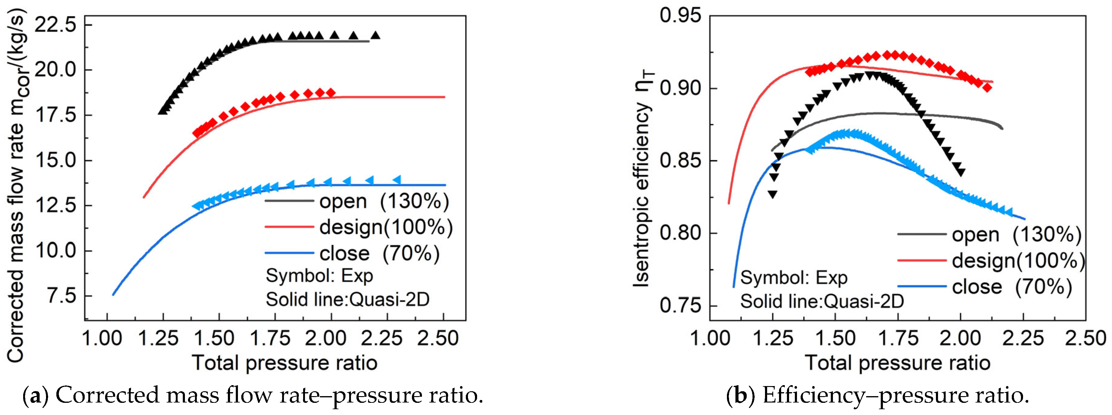
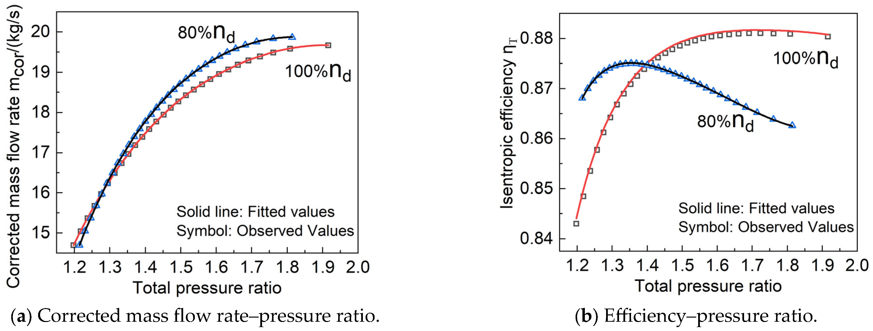
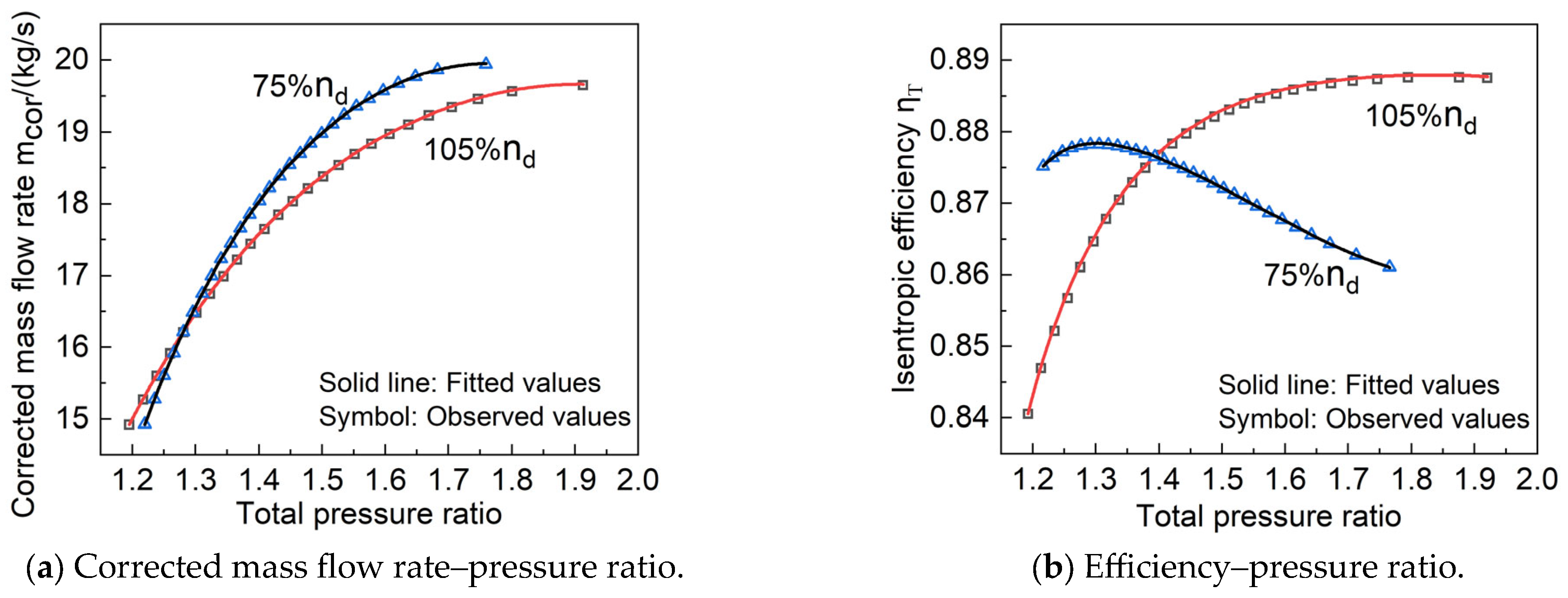
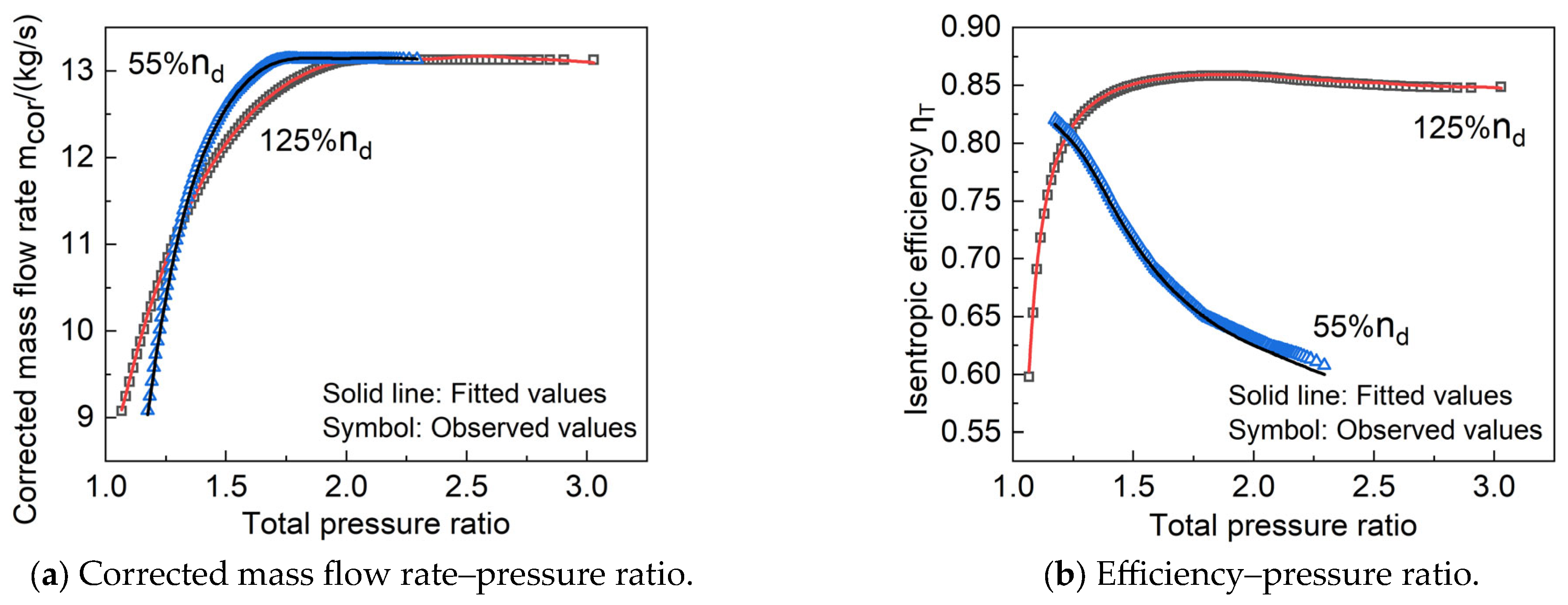
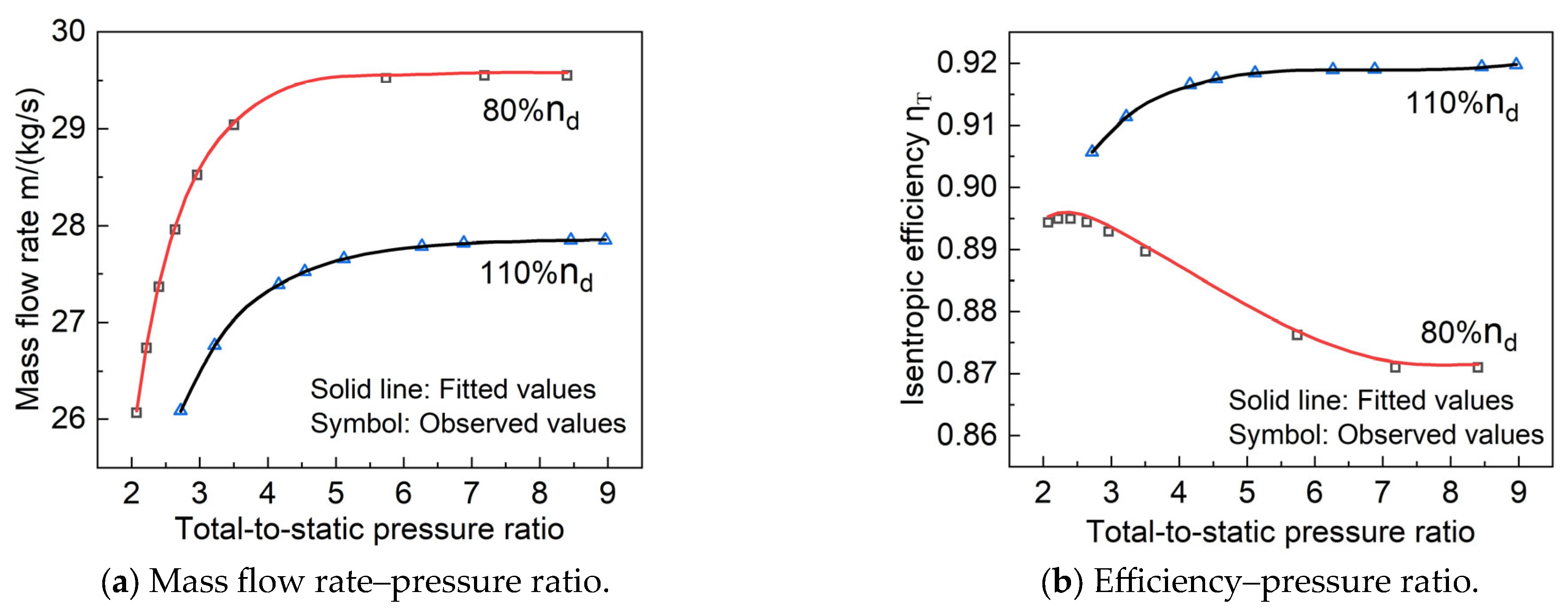
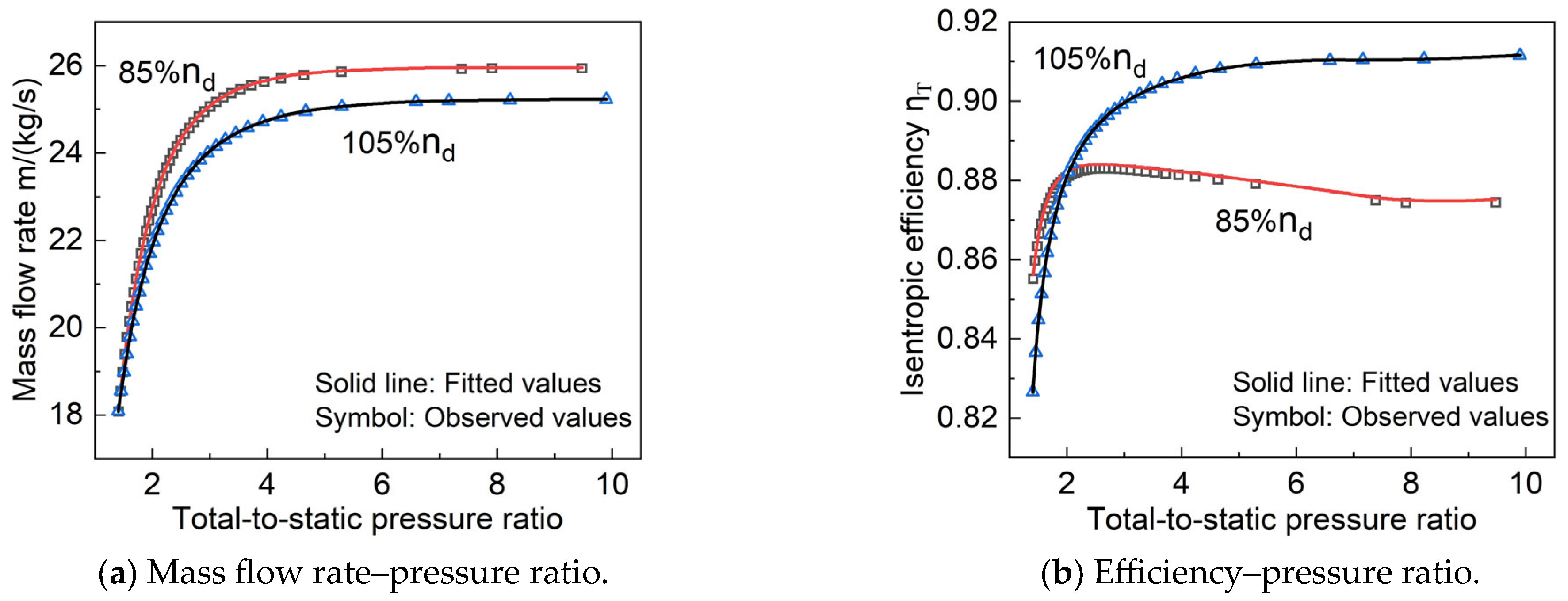
• A quasi-2D performance prediction method for axial flow turbines was developed using a simple radial equilibrium equation to consider variation in aerodynamic parameters along the spanwise direction. At 40%, 70%, and 100% design speeds, the maximum relative errors of the single-stage turbine corrected mass flow rate and efficiency were 0.7% and 4.44%, respectively. At 70%, 100%, and 110% design speeds, the maximum relative errors of the five-stage turbine mass flow rate and efficiency did not exceed 1.67% or 1.385%, respectively. This shows that the method reliably and accurately predicts turbine performance.
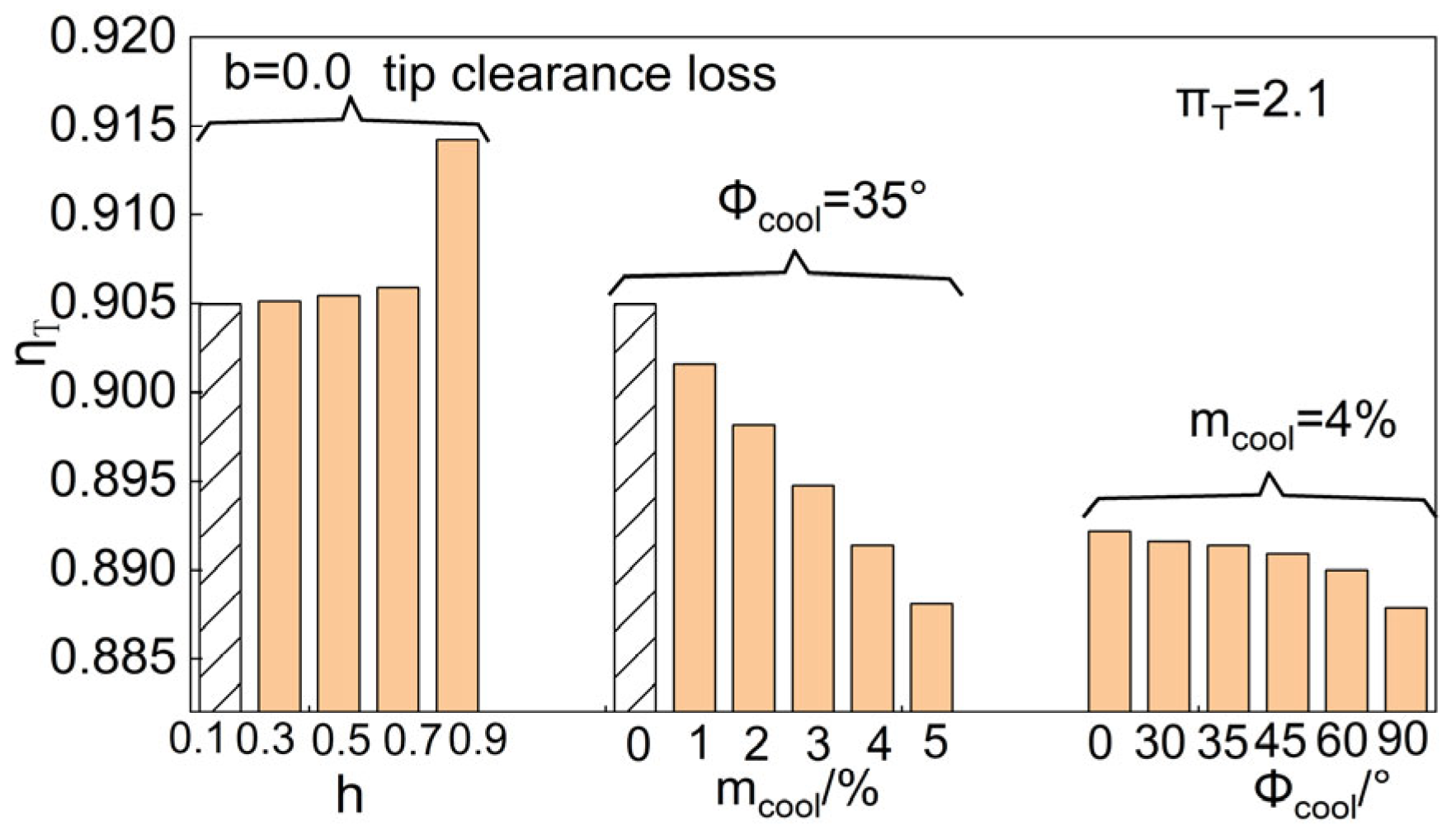
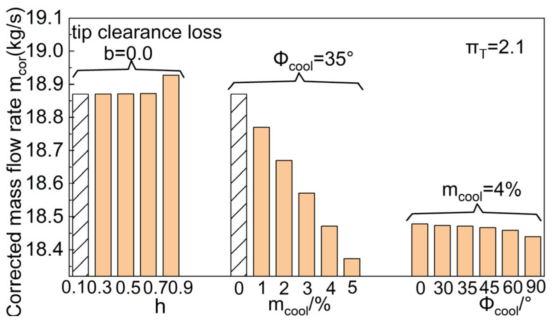
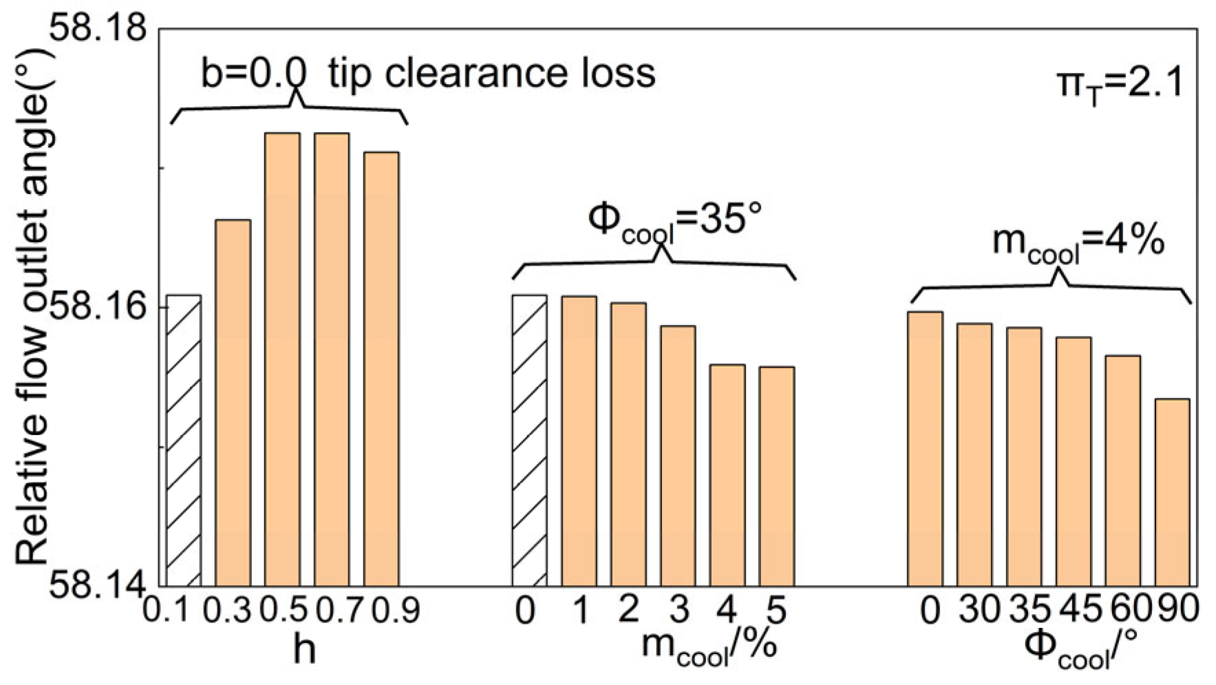
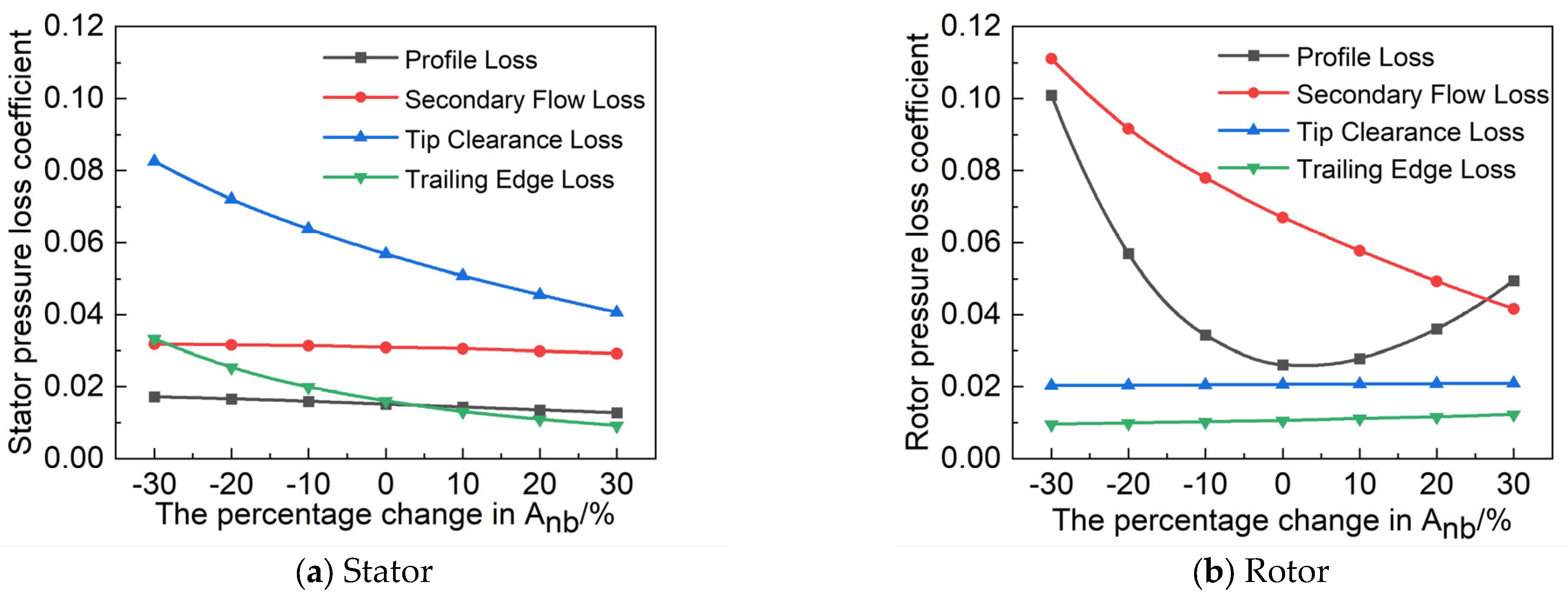
• A sensitivity analysis of the single-stage turbine was conducted. When conducting research based on the quasi-2D method and adopting the K-O loss model, the radial distribution patterns of secondary flow loss and tip clearance loss had low sensitivity to efficiency and the mass flow rate. It is reasonable to use the parabolic distribution pattern for the radial distribution of secondary flow loss and tip clearance loss.
• The quasi-2D axial flow turbine variable geometry performance prediction method was further developed. The maximum relative errors of the single-stage turbine corrected mass flow rate under 130%, 100%, and 70% design areas were 1.362%, 2.242%, and 3.602%, respectively, and the maximum relative errors of turbine efficiency were 4.228%, 1.139%, and 1.253%, respectively. This indicates that the variable geometry turbine performance prediction method developed in this study is highly accurate.
• Both opening and closing A_nb will cause a decrease in turbine efficiency and closing A_nb causes a greater decrease in turbine efficiency. The change in mass flow rate is smaller than the change in A_nb. When the pressure ratio is 1.75, the A_nb of the single-stage turbine is closed by 30%, the efficiency decreases by 6.932%, and the m_cor decreases by 25.67%; when A_nb is opened up by 30%, the turbine efficiency decreases by 3.148% and m_cor decreases by 19.48%. When the design total-to-static pressure ratio is 4.76, the A_nb of the five-stage turbine is opened up by 20%, the turbine efficiency decreases by 0.116% and the m increases by 4.62%; when A_nb is closed by 20%, the turbine efficiency decreases by 1.653% and m decreases by 10.10%.
• A surrogate model of variable geometry turbine performance considering the effect of cooling air was constructed based on a BP neural network. The BP neural network models established for the single-stage and five-stage turbines had R² values greater than 0.999 for the training samples. The MAPE predicted for the known performance data did not exceed 0.04%; the MAPE predicted for the performance data within the sample space range did not exceed 0.04%; and the MAPE predicted for the performance data outside the sample space range did not exceed 0.43%. This indicates that the surrogate model established in this study has high prediction accuracy and strong generalization ability.

References

1. Behning, F.P.; Moffitt, T.P.; Schum, H.J. Effect of Variable Stator Area on Performance of a Single-Stage Turbine Suitable for Air Cooling. 3—Turbine Performance with 130-Percent Design Stator Area; NASA Report No. NASA-TM-X-1663; Lewis Research Center: Cleveland, OH, USA, 1968. [Google Scholar]
2. Prust, H.W.; Schum, H.J.; Szanca, E.M. Effect of Variable Stator Area on Performance of a Single-Stage Turbine Suitable for Air Cooling. 6—Turbine Performance with 70-Percent Design Stator Area; NASA Report No. NASA-TM-X-1697; Lewis Research Center: Cleveland, OH, USA, 1968. [Google Scholar]
3. Moffitt, T.; Schum, H. Performance of a single-stage turbine as affected by variable statorarea. In Proceedings of the 5th Propulsion Joint Specialist, Colorado Springs, CO, USA, 9–13 June 1969. [Google Scholar] [CrossRef]
4. Behning, F.P.; Schum, H.J.; Szanca, E.M. Cold-Air Investigation of a Turbine for High Temperature-Engine Application. 5: Two-Stage Turbine Performance as Affected by Variable Stator Area; NASA Report No. NASA-TN-D-4389; Lewis Research Center: Cleveland, OH, USA, 1974. [Google Scholar]
5. Kozak, D.; Mazuro, P.; Teodorczyk, A. Numerical Simulation of Two-Stage Variable Geometry Turbine. Energies 2021, 14, 5349. [Google Scholar] [CrossRef]
6. Galindo, J.; Tiseira, A.; Fajardo, P.; García-Cuevas, L.M. Development and validation of a radial variable geometry turbine model for transient pulsating flow applications. Energy Convers. Manag. 2014, 85, 190–203. [Google Scholar] [CrossRef]
7. Razinsky, E.H.; Kuziak, W.R., Jr. Aerothermodynamic Performance of a Variable Nozzle Power Turbine Stage for an Automotive Gas Turbine. J. Eng. Power 1977, 99, 587–592. [Google Scholar] [CrossRef]
8. Yao, Y.; Tao, Z.; Zhou, K.; Yang, Y.; Song, L.; Li, J.; Feng, Z. Aerodynamic performance measurement of a novel variable geometry turbine adjustable guide vane scheme by experimental study. Aerosp. Sci. Technol. 2023, 140, 108413. [Google Scholar] [CrossRef]
9. Yue, G.; Lin, H.; Jiang, Y.; Zheng, Q.; Dong, P. Effect of Tip Configurations on Aerodynamic Performance of Variable Geometry Linear Turbine Cascade. Int. J. Turbo Jet-Engines 2019, 36, 457–470. [Google Scholar] [CrossRef]
10. Niu, X.; Liang, C.; Jing, X.; Wei, J.; Zhu, K. Experimental Investigation of Variable Geometry Turbine Annular Cascade for Marine Gas Turbines. In American Society of Mechanical Engineers Digital Collection; AMSE: New York, NY, USA, 2016. [Google Scholar] [CrossRef]
11. Orkisz, M.; Stawarz, S. Modeling of Turbine Engine Axial-Flow Compressor and Turbine Performance. J. Propuls. Power 2000, 16, 336–339. [Google Scholar] [CrossRef]
12. Liu, Z.; Karimi, I.A. Gas turbine performance prediction via machine learning. Energy 2020, 192, 116627. [Google Scholar] [CrossRef]
13. Lazzaretto, A.; Andrea, T. Analytical and Neural Network Models for Gas Turbine Design and Off-Design Simulation. Int. J. Thermodyn. 2001, 4, 173–182. [Google Scholar] [CrossRef]
14. Bartolini, C.M.; Caresana, F.; Comodi, G.; Pelagalli, L.; Renzi, M.; Vagni, S. Application of artificial neural networks to micro gas turbines. Energy Convers. Manag. 2011, 52, 781–788. [Google Scholar] [CrossRef]
15. Cortés, O.; Urquiza, G.; Hernández, J.A. Optimization of operating conditions for compressor performance by means of neural network inverse. Appl. Energy 2009, 86, 2487–2493. [Google Scholar] [CrossRef]
16. Ghorbanian, K.; Gholamrezaei, M. An artificial neural network approach to compressor performance prediction. Appl. Energy 2009, 86, 1210–1221. [Google Scholar] [CrossRef]
17. Li, B.; Gu, C.; Li, X.; Liu, T. Numerical optimization for stator vane settings of multi-stage compressors based on neural networks and genetic algorithms. Aerosp. Sci. Technol. 2016, 52, 81–94. [Google Scholar] [CrossRef]
18. Liu, C.; Zou, Z.; Xu, P.; Wang, Y. Development of helium turbine loss model based on knowledge transfer with neural network and its application on aerodynamic design. Energy 2024, 297, 131327. [Google Scholar] [CrossRef]
19. Galindo, J.; Luján, J.M.; Serrano, J.R.; Hernández, L. Combustion simulation of turbocharger HSDI Diesel engines during transient operation using neural networks. Appl. Therm. Eng. 2005, 25, 877–898. [Google Scholar] [CrossRef]
20. Serrano, J.R.; Piqueras, P.; De la Morena, J.; Gómez-Vilanova, A.; Guilain, S. Methodological analysis of variable geometry turbine technology impact on the performance of highly downsized spark-ignition engines. Energy 2021, 215, 119122. [Google Scholar] [CrossRef]
21. Serrano, J.; Climent, H.; Navarro, R.; González-Domínguez, D. Methodology to Standardize and Improve the Calibration Process of a 1D Model of a GTDI Engine; SAE International: Warrendale, PA, USA, 2020. [Google Scholar] [CrossRef]
22. Park, Y.; Choi, M.; Kim, K.; Li, X.; Jung, C.; Na, S.; Choi, G. Prediction of operating performance for industrial gas turbine combustor using an optimized artificial neural network. Energy 2020, 213, 118769. [Google Scholar] [CrossRef]
23. Nikpey, H.; Assadi, M.; Breuhaus, P. Development of an optimized artificial neural network model for combined heat and power micro gas turbines. Appl. Energy 2013, 108, 137–148. [Google Scholar] [CrossRef]
24. Campora, U.; Cravero, C.; Zaccone, R. Marine gas turbine monitoring and diagnostics by simulation and pattern recognition. Int. J. Nav. Archit. Ocean. Eng. 2018, 10, 617–628. [Google Scholar] [CrossRef]
25. Bettocchi, R.; Pinelli, M.; Spina, P.R.; Venturini, M. Artificial Intelligence for the Diagnostics of Gas Turbines—Part I: Neural Network Approach. J. Eng. Gas Turbines Power 2006, 129, 711–719. [Google Scholar] [CrossRef]
26. Fast, M.; Assadi, M.; De, S. Development and multi-utility of an ANN model for an industrial gas turbine. Appl. Energy 2009, 86, 9–17. [Google Scholar] [CrossRef]
27. Park, Y.; Choi, M.; Choi, G. Fault detection of industrial large-scale gas turbine for fuel distribution performance in start-up procedure using artificial neural network method. Energy 2022, 251, 123877. [Google Scholar] [CrossRef]
28. Rahmoune, M.B.; Hafaifa, A.; Kouzou, A.; Chen, X.; Chaibet, A. Gas turbine monitoring using neural network dynamic nonlinear autoregressive with external exogenous input modelling. Math. Comput. Simul. 2021, 179, 23–47. [Google Scholar] [CrossRef]
29. Flagg, E.E. Analytical Procedure and Computer Program for Determining the Off-Design Performance of Axial Flow Turbines; NASA Report No. NASA-CR-710; Lewis Research Center: Cleveland, OH, USA, 1967. [Google Scholar]
30. Kacker, S.C.; Okapuu, U. A Mean Line Prediction Method for Axial Flow Turbine Efficiency. J. Eng. Power 1982, 104, 111–119. [Google Scholar] [CrossRef]
31. Ainley, D.G.; Mathieson, G.C.R. A Method of Performance Estimation for Axial-Flow Turbines; A.R.C. Technical Report No. 2974; Ministry of Supply: London, UK, 1951. [Google Scholar]
32. Glassman, A.J. Modeling Improvements and Users Manual for Axial-Flow Turbine Off-Design Computer Code AXOD; NASA Report No. NASA-CR-195370; Lewis Research Center: Cleveland, OH, USA, 1994. [Google Scholar]
33. Chen, S.-C.S. A Guide to Axial-Flow Turbine Off-Design Computer Program AXOD2; NASA Report No. NASA/TM-2014-218301; Lewis Research Center: Cleveland, OH, USA, 2014. [Google Scholar]
34. Hanley, W.T. A Correlation of End Wall Losses in Plane Compressor Cascades. J. Eng. Power 1968, 90, 251–257. [Google Scholar] [CrossRef]
35. Tabakoff, W. An experimental investigation on loss reduction in small guide vanes. In Proceedings of the 12th Propulsion Conference, Palo Alto, CA, USA, 26–29 July 1976. [Google Scholar] [CrossRef]
36. Sullerey, R.K.; Kumar, S. A Study of Axial Turbine Loss Models in a Streamline Curvature Computing Scheme. J. Eng. Gas Turbines Power 1984, 106, 591–597. [Google Scholar] [CrossRef]
37. de Jesus, G.S.; Barbosa, J.R.; Ramsden, K.W. A Comparison of Loss Models Using Different Radial Distribution of Loss in an Axial Turbine Streamline Curvature Program. In American Society of Mechanical Engineers Digital Collection; AMSE: New York, NY, USA, 2009; pp. 685–692. [Google Scholar] [CrossRef]
38. Ito, S.; Eckert, E.R.G.; Goldstein, R.J. Aerodynamic Loss in a Gas Turbine Stage with Film Cooling. J. Eng. Power 1980, 102, 964–970. [Google Scholar] [CrossRef]
39. Hartsel, J. Prediction of effects of mass-transfer cooling on the blade-row efficiency of turbine airfoils. In Proceedings of the 10th Aerospace Sciences Meeting, San Diego, CA, USA, 17–19 January 1972. [Google Scholar] [CrossRef]
40. Bider, B.; Monroe, D.E.; Szanca, E.M.; Whitney, W.J. Cold-Air Investigation of a Turbine for High-Temperature-Engine Application. 3—Overall Stage Performance; NASA Report No. NASA/TN-D-4389; Lewis Research Center: Cleveland, OH, USA, 1968. [Google Scholar]
41. Moffitt, T.P.; Monroe, D.E.; Szanca, E.M.; Whitney, W.J. Cold-Air Investigation of a Turbine For High-Temperature-Engine Application; NASA Report No. NASA/TN-D-3751; Lewis Research Center: Cleveland, OH, USA, 1967. [Google Scholar]
42. Cherry, D.G.; Gay, C.H.; Lenahan, D.T. Energy Efficient Engine. Low Pressure Turbine Test Hardware Detailed Design Report; NASA Report No. NASA-CR-167956; Lewis Research Center: Cleveland, OH, USA, 1982. [Google Scholar]
43. Bridgeman, M.J.; Cherry, D.G.; Pedersen, J. NASA/GE Energy Efficient Engine Low Pressure Turbine Scaled Test Vehicle Performance Report; NASA Report No. NASA-CR-168290; Lewis Research Center: Cleveland, OH, USA, 1983. [Google Scholar]
Figure 1. Schematic diagram of a single-stage turbine calculation station.
Aerospace 12 00410 g001
Figure 2. Calculation of stator blade aerodynamic parameters.
Aerospace 12 00410 g002
Figure 3. Calculation of multi-stage turbine performance.
Aerospace 12 00410 g003
Figure 4. The distribution of losses along the span.
Aerospace 12 00410 g004
Figure 5. The choking iteration process of a blade row.
Aerospace 12 00410 g005
Figure 6. Schematic diagram of variation in turbine guide stagger angle [1,2,3].
Aerospace 12 00410 g006
Figure 7. Variation in RMSE with the number of nodes in the hidden layer.
Aerospace 12 00410 g007
Figure 8. Single-stage turbine performance.
Aerospace 12 00410 g008
Figure 9. Five-stage turbine performance.
Aerospace 12 00410 g009
Figure 10. Sensitivity of secondary flow loss distribution to turbine performance.
Aerospace 12 00410 g010
Figure 11. Sensitivity of radial distribution of tip clearance loss, m c o o l and ϕ c o o l to ηT.
Aerospace 12 00410 g011
Figure 12. Sensitivity of radial distribution of tip clearance loss, m c o o l and ϕ c o o l to m c o r .
Aerospace 12 00410 g012
Figure 13. Sensitivity of radial distribution of tip clearance loss, m c o o l and ϕ c o o l to relative flow outlet angle.
Aerospace 12 00410 g013
Figure 14. Single-stage turbine variable geometry performance.
Aerospace 12 00410 g014
Figure 15. The variation law of loss with A n b .
Aerospace 12 00410 g015
Figure 16. Variable geometry performance of a five-stage turbine.
Aerospace 12 00410 g016
Figure 17. Fitting ability of BP neural network for known data ( Δ γ = 3 ° , m c o o l = 3 % ).
Aerospace 12 00410 g017
Figure 18. Interpolation ability of BP neural network ( Δ γ = 3.5 ° , m c o o l = 1.5 % ).
Aerospace 12 00410 g018
Figure 19. Extrapolation ability of BP neural network ( Δ γ = 6.5 ° , m c o o l = 6.5 % ).
Aerospace 12 00410 g019
Figure 20. Fitting ability of BP neural network for known data ( Δ γ = 6 ° , m c o o l = 2 % ).
Aerospace 12 00410 g020
Figure 21. Interpolation performance of BP neural network ( Δ γ = 5 ° , m c o o l = 3 % ).
Aerospace 12 00410 g021
Figure 22. Extrapolation performance of BP neural network ( Δ γ = 8.5 ° , m c o o l = 9 % ).
Aerospace 12 00410 g022