A Review of Wavefront Sensing and Control Based on Data-Driven Methods

Abstract

Optical systems suffer from wavefront aberrations due to complex atmospheric environments and system component errors, leading to systematic aberrations and significantly degrading optical field quality. Therefore, the detection and correction of optical aberrations are crucial for efficient and accurate observations. To fully utilize the capabilities of observation equipment and achieve high-efficiency, accurate imaging, it is essential to develop wavefront correction technologies that enable ultra-precise wavefront control. The application of data-driven techniques in wavefront correction can effectively enhance correction performance and better address complex environmental challenges. This paper elaborates on the research progress of data-driven methods in wavefront correction from three aspects: principles, current research status, and practical applications. It analyzes the performance of data-driven methods in diverse real-world scenarios and discusses future trends in the deep integration of data-driven approaches with optical technologies. This work provides valuable guidance for advancing wavefront correction methodologies.

1. Introduction

Large-aperture survey telescopes have facilitated large-scale and detailed explorations of the universe. The international astronomical community has achieved substantial progress in astronomical surveys and observations over the years, and space telescopes, such as the Hubble Space Telescope and James Webb Space Telescope, play important roles in this field. In the near future, the China Space Station Telescope (CSST) will be launched and produce scientific results. Some of the major large-aperture survey telescopes currently in operation include China’s Extremely Large Spectroscopic Survey Telescope (ESST), Multiplexed Survey Telescope (MUST), the European Extremely Large Telescope (E-ELT), the Giant Magellan Telescope (GMT), and the Thirty Meter Telescope (TMT). To enable direct imaging of exoplanets, the upcoming generation of 30 m-class telescopes demands ultra-high-precision wavefront control. Multi-band, high-frequency time-domain surveys with a large field of view (FOV) are essential for efficiently searching for and monitoring celestial dynamic events. Additionally, high-performance observation instruments and the capacity to fully exploit their observation capabilities are indispensable. Consequently, the realization of a new generation of extremely large survey telescopes depends heavily on reconstructing complex wavefronts and controlling system aberrations.

The aperture of current mirrors is constrained by limitations in manufacturing technology, which restricts the aperture and FOV of spectroscopic survey telescopes. The use of segmented mirrors enhances the observational capabilities of telescopes, but achieving this requires sub-mirrors to maintain extremely high co-phase accuracy. Moreover, light propagating through turbulent space media causes blurring, leading to distorted wavefront distributions. The imaging detector captures only intensity information and lacks phase data, necessitating wavefront sensing techniques to reconstruct the wavefront phase. This involves predicting the wavefront phase from the image intensity, addressing the nonlinear relationship between intensity and phase. Most wavefront sensors (WFSs) exhibit nonlinear characteristics, and precise wavefront reconstruction necessitates nonlinear reconstruction techniques. Machine learning-based data analysis methods, characterized by their asymmetry, offer flexibility and adaptability. These methods enable the automated development of analytical models that correlate image intensity with phase and amplitude information of the incident wavefront. In segmented mirror telescopes, relative position errors between sub-mirrors can arise, particularly in space-based telescopes, where external disturbances, thermal deformation, gravitational deformation, spacecraft jitter, and other factors exacerbate these errors. Maintaining the optical path length between sub-apertures to within a small fraction of the wavelength is critical; otherwise, imaging resolution decreases significantly. By employing deep learning to measure system aberrations, imaging performance can be optimized, achieving resolutions comparable to telescopes with monolithic primary mirrors and resulting in higher observational resolutions. Data-driven methods leverage the asymmetry of neural networks to transform linear correspondences into nonlinear relationships, marking a shift from rule-driven to data-driven approaches. This enables the rapid estimation and accurate prediction of wavefront phase information.

Comparison between Rule-Driven and Data-Driven Methods. Rule-driven methods exhibit high transparency and strong interpretability but suffer from low flexibility. They are suitable for well-defined problem domains where rules can be exhaustively defined and stability is ensured. However, rule-driven approaches fail to handle novel scenarios outside predefined rules and struggle to capture complex nonlinear relationships. In contrast, data-driven methods demonstrate high adaptability but are data-dependent and lack interpretability. They can automatically learn high-dimensional, nonlinear features, reduce human intervention, and are ideal for automated decision-making. Through incremental learning, they adapt to evolving data distributions and enable continuous learning. However, these methods require substantial computational resources, and training complex models demands high-performance hardware support. Considering the potential significant reduction in hardware costs in the future, coupled with the widespread adoption of supercomputers and GPUs, data-driven methods will demonstrate distinct advantages in addressing nonlinear challenges for next-generation ultra-large-scale and ultra-precision optical applications. By strategically selecting or integrating both approaches, an optimal balance among efficiency, accuracy, and robustness can be achieved.

This paper discusses issues related to high-resolution imaging and system aberration control. In the high-resolution imaging section, several typical wavefront sensors (WFSs) and holography techniques are investigated, along with their integration effects with machine learning. Regarding system aberration control, the study explores aspects such as piston detection, aberration suppression, and smart focusing elements, highlighting the effectiveness of data-driven approaches in system aberration correction.

2. High-Resolution Imaging

High-resolution imaging is a vital technique for the direct detection and characterization of exoplanets, integrating ground-based extreme adaptive optics (AO) with coronagraphy. So far, around 30 exoplanets have been discovered using high-contrast imaging methods. However, most of these are gas giants, with masses multiple times that of Jupiter. A key challenge in improving sensitivity is the correction of non-common path aberrations (NCPAs). These quasi-static aberrations, evolving over minutes to hours, stem from instrumental instabilities influenced by changes in temperature, humidity, and gravity vectors. Since these aberrations occur downstream of the wavefront sensor (WFS), they cannot be corrected by conventional wavefront control systems. Consequently, further advancements in wavefront control methods are required. Zernike polynomials, introduced by Frits Zernike in 1934, offer an effective mathematical tool for representing the phase distribution of wavefronts. These polynomials have become a cornerstone in modeling atmospheric turbulence in astronomy.

AO technology is underpinned by a well-established theoretical framework, and essential components such as wavefront detectors, processors, and correctors have been developed [1]. Adaptive optics (AO) systems are developed to correct dynamic wavefront aberrations in real time. These corrections involve translating wavefront measurements into control signals for deformable mirror (DM) actuators, which compensate for aberrations by restoring the wavefront to its planar form. To optimize DM actuator commands, precise phase measurements across the entire wavefront are essential. Reconstructing the wavefront from WFS data presents an inverse problem, and the solution depends on the type of WFS used.

2.1. Shack–Hartmann Wavefront Sensor (SHWFS)

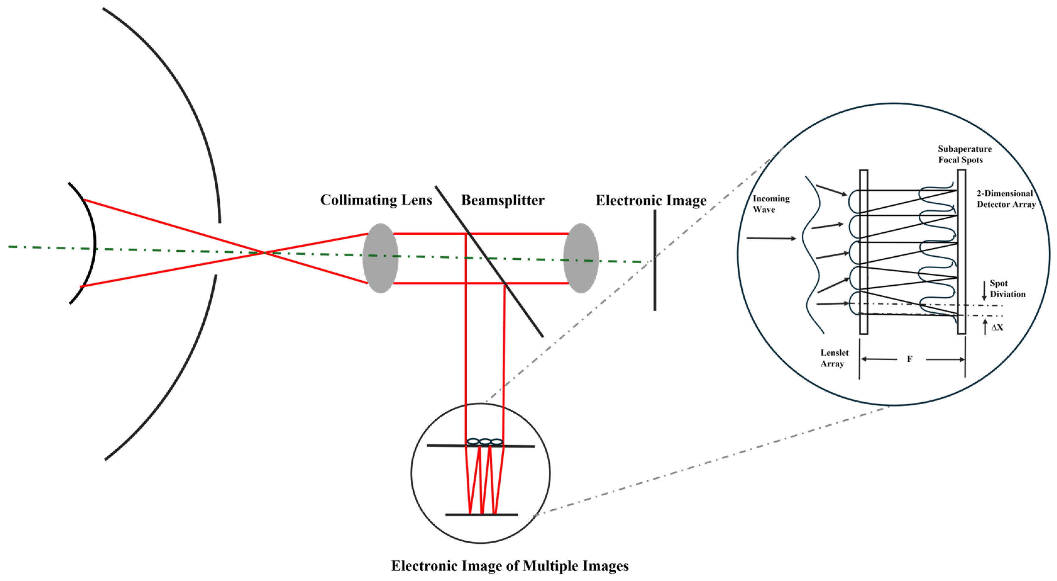
Shack–Hartmann wavefront sensors (SHWFSs) are extensively used in applications such as astronomy, high-energy lasers, funduscopic imaging, optical communications, and optical detection due to their straightforward physical principles, high light energy utilization, fast detection speeds, and stable performance. An SHWFS comprises a lenslet array and a two-dimensional detector, with each lenslet functioning as a sub-aperture. The lenslet array divides the beam into multiple spatially independent sub-beams and focuses them separately onto the two-dimensional detector. The distribution of each focal point corresponds to the localized wavefront slope on each lenslet. The average wavefront slope is determined by calculating the displacement of each centroid relative to an aberration-free reference. Using wavefront reconstruction algorithms, such as modal or zonal methods, the overall wavefront can be reconstructed from these slopes. However, the accuracy of Shack–Hartmann Wavefront Sensors (SHWFSs) is limited by centroid positioning errors and the average wavefront slope. Furthermore, the spot intensity distribution contains valuable information that can be exploited more effectively, simplifying the wavefront detection process. The configuration of SHWFS is shown in Figure 1. It illustrates the measurement of light spot displacements formed by the lens array to calculate wavefront tilt. The derivative of the wavefront optical path difference (OPD) plot yields the wavefront slope, whereas the integral of the wavefront slope reconstructs the wavefront OPD plot.

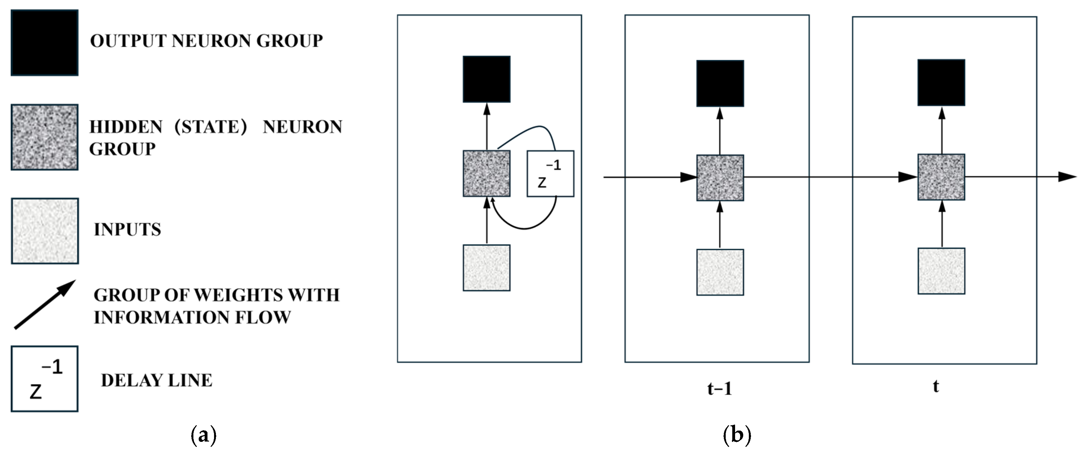
Deep learning methods, especially Convolutional Neural Networks (CNNs) and Recurrent Neural Networks (RNNs), have found wide applications in Adaptive Optics (AO) wavefront reconstruction [2]. A Recurrent Neural Network (RNN) is a type of neural sequence model commonly used for sequential data problems. It captures correlations between proximate data points in a sequence, making it well-suited for handling the temporal aspects of prediction and control tasks. As shown in Figure 2, a basic RNN architecture features delay lines and is unfolded over two time steps. In this structure, input vectors are fed into the RNN sequentially, enabling the architecture to leverage all available input information up to the current time step for prediction. The amount of information captured by a specific RNN depends on its architecture and training algorithm. Common variants of RNNs include Long Short-Term Memory (LSTM) networks [3] and Gated Recurrent Units (GRUs).

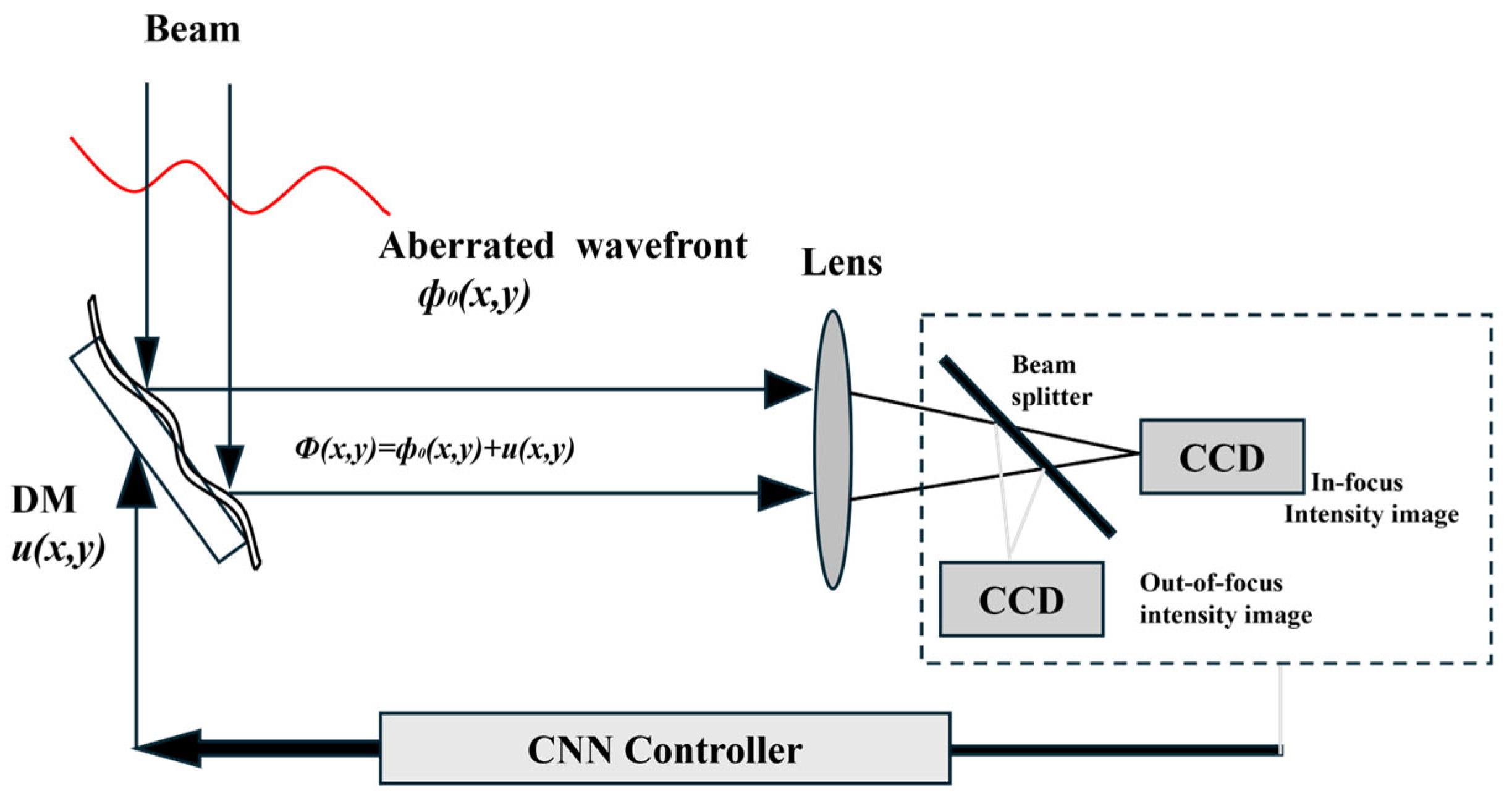
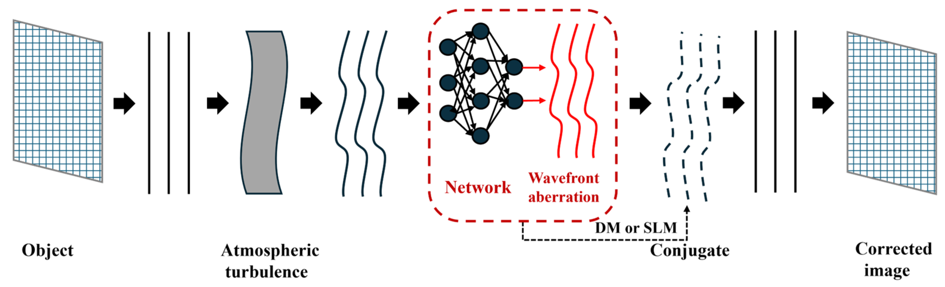
Studies show that CNNs can efficiently and accurately estimate Zernike coefficients from SHWFS patterns. Figure 3 illustrates the architecture of a CNN-based AO system. CNNs learn the mapping between light intensity images and Zernike coefficients for wavefront reconstruction. A typical CNN model consists of an input layer, multiple convolutional layers, pooling layers, fully connected layers, a SoftMax classifier, and an output layer. The network employs a series of transformation layers to extract features from the input image or patch, enabling the classification of the input data.

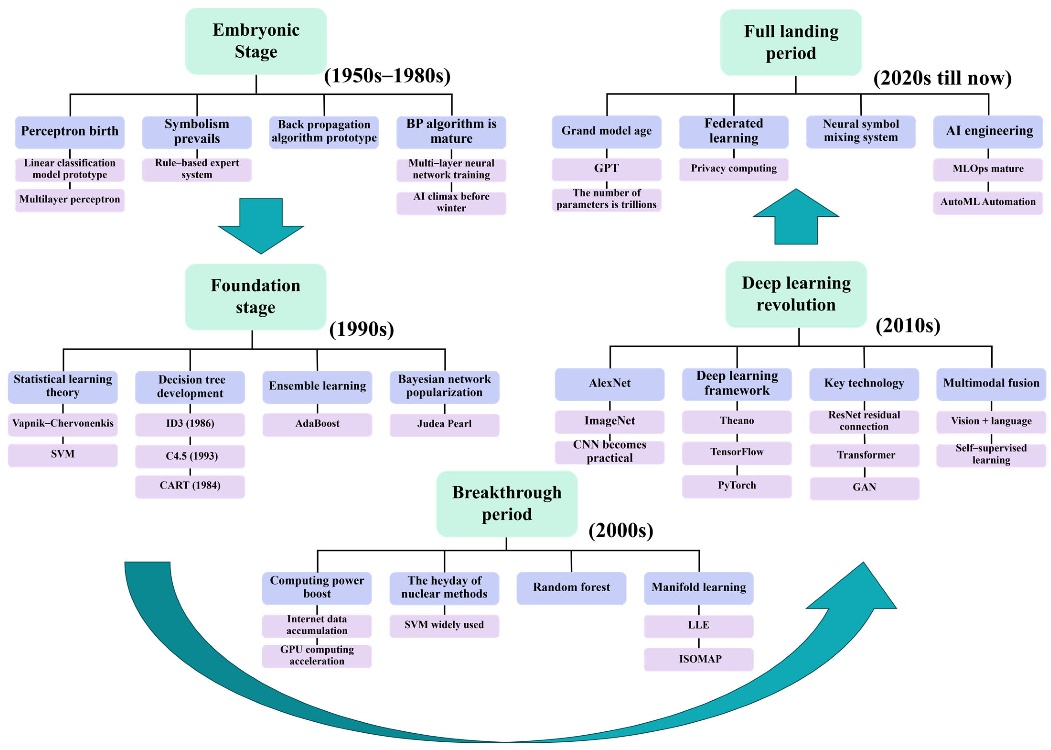
Figure 4 illustrates the development trends of machine learning from the 1950s to the present. Machine learning-based data-driven methods take input sequences of light spot position coordinates (e.g., centroid displacements of sub-apertures) and directly predict wavefront phase distributions (such as Zernike coefficients or complex amplitude distributions). Examples include the following:

• U-Net architecture enables end-to-end reconstruction networks, where inputting light spot images predicts wavefront phases. Compared to traditional least squares methods, phase errors are reduced by 50%.
• YOLO or Faster R-CNN object detection networks replace traditional centroid detection, improving sub-pixel level localization accuracy.
• Generative adversarial networks (GANs) or autoencoders for denoising algorithms recover clean light spot images without relying on physical models.
• Anomaly detection in light spot distribution patterns (e.g., missing spots or displacements exceeding thresholds) triggers alarms for microlens damage identification. Global displacement analysis localizes mechanical shifts or thermal drifts in microlens arrays, enabling misalignment diagnostics.

Data-driven approaches enable real-time optimization of dynamic wavefront correction. Embedding LSTM networks into adaptive optics closed-loop systems predicts dynamic wavefront trends, enhancing correction speed. Combined with GPU/FPGA acceleration (e.g., lightweight models like ResNet), inference latency achieves sub-millisecond response. In turbulence simulation experiments, dynamic correction latency is reduced from 100 ms (traditional methods) to 5 ms, significantly improving imaging stability.

Guo et al. successfully reconstructed distorted wavefronts using an artificial neural network, wherein wavefront information was derived from the spot displacement of SHWFS apertures [4]. Osborn et al. implemented open-loop wavefront reconstruction for a multi-object AO system using a fully connected neural network [5]. Swanson et al. proposed a CNN with a U-Net architecture for wavefront reconstruction, enabling the direct generation of 2D wavefront phase maps using wavefront slope as input. Additionally, they utilized an RNN with LSTM architecture to predict wavefront phase maps up to five steps into the future [6]. Li et al. developed a Hartmann sensor with the detector placed at the defocused plane of the lenslet [7]. The Shack–Hartmann sensor is enhanced by positioning a detector at a defocused plane located upstream of the microlens array’s focal plane. The phase retrieval algorithm employs a hybrid optimization framework, initializing Zernike coefficients through conventional Shack–Hartmann-based phase reconstruction and further refining them via stochastic parallel-gradient descent. This approach effectively recovers wavefront aberrations while significantly improving convergence efficiency compared to traditional methods.

In 2018, Ma et al. modified the AlexNet network structure [8] to simulate and generate focal and defocused images of atmospheric turbulence at varying intensities. AlexNet, a landmark deep neural network in computer vision, features a hierarchical architecture comprising five convolutional layers (with max-pooling operations applied after certain layers to reduce spatial redundancy) and three fully connected layers, culminating in a 1000-class softmax classifier. The network contains 60 million parameters and 650,000 neurons, leveraging ReLU activation functions for accelerated training and dropout regularization to mitigate overfitting. Its design marked a pivotal advancement in deep learning, achieving state-of-the-art performance on the ImageNet Large Scale Visual Recognition Challenge (ILSVRC) in 2012. These images were used to train a model to predict the first 35 Zernike coefficients [9]. In the same year, Paine [10] employed the Inception v3 network architecture to estimate wavefront phases based solely on focal-plane intensity images [11]. Inception-v3 enhances computational efficiency by decomposing traditional 7 × 7 convolutions into three parallel 3 × 3 convolutional branches within Inception modules, reducing spatial redundancy while preserving feature diversity. The network employs three hierarchical Inception modules (each with 288 filters) at a 35 × 35 resolution stage, followed by mesh reduction layers to progressively downsample the feature maps to a 17 × 17 grid with 768 filters. Experimental results demonstrate that this architecture achieves state-of-the-art accuracy in wavefront aberration prediction, outperforming conventional CNNs by reducing phase estimation errors by 32% in optical coherence tomography (OCT) imaging tasks. In 2019, Nishizaki et al. employed a CNN-based neural network to compute the first 32 Zernike coefficients from a single-intensity image [12]. In 2020, Wu et al. predicted the first 13 Zernike coefficients using a PD-CNN structure, utilizing focal and defocused images as inputs to the network [13].

Phase diversity (PD) offers a simpler optical configuration with no non-common-path aberrations, making it inherently robust for computational imaging tasks. Its primary applications lie in post-processing of blurred images and scenarios with lower real-time constraints, such as offline data analysis or scientific imaging systems.

The PD-CNN architecture adopts a hierarchical design consisting of:

• Three convolutional layers (with ReLU activation for feature extraction),
• Three max-pooling layers (for spatial dimensionality reduction),
• Two fully connected layers (ending in a softmax classifier for regression or classification tasks).

This structure balances computational efficiency with feature learning capabilities, achieving sub-pixel level accuracy in phase retrieval tasks while maintaining compatibility with PD’s inherent optical simplicity.

Accurate wavefront measurement at the scientific focal plane is vital for applications such as the direct imaging of exoplanets. In 2019, Vanberg et al. [14] evaluated the efficiency of neural architectures on two datasets, investigating the use of modern CNN architectures—such as ResNet, InceptionV3, U-Net, and U-Net++—for estimating and correcting NCPAs.

They employ Inception V3 and ResNet-50 neural networks to estimate a set of modal coefficients, while U-Net and U-Net++ architectures are used for direct phase diagram reconstruction. Training is conducted using stochastic gradient descent with momentum. The Inception V3 and ResNet-50 models are initialized with pretrained weights, whereas the U-Net and U-Net++ architectures are instantiated with Xavier initialization.

Table 1. Summary of final performance expressed as RMSE between exact and estimated phase maps (in radians).

Architecture	20 Zernike	100 Zernike	Inference Time
Inception V3	0.0240 $\pm$ 0.0051	0.1094 $\pm$ 0.0154	0.1182 s
ResNet 50	0.0187 $\pm$ 0.0039	0.1145 $\pm$ 0.0138	0.1090 s
Unet	0.0132 $\pm$ 0.0019	0.0976 $\pm$ 0.0109	0.1102 s
Unet++	0.0130 $\pm$ 0.0023	0.0943 $\pm$ 0.0133	0.1358 s

demonstrates that direct phase reconstruction outperforms modal coefficient estimation. For the optimal ResNet/U-Net++ architectures:

• On the first dataset (generated with 20 Zernike modes), the overall improvement is 36% (or 2 nm RMS error reduction).
• On the second dataset (generated with 100 Zernike modes), the improvement reaches 19% (or 7 nm RMS error reduction).

This highlights the superiority of end-to-end phase reconstruction over iterative coefficient-based methods, particularly in high-dimensional Zernike mode scenarios.

The point spread functions (PSFs) are as follows:

$$PSF(x,y)={\displaystyle \iint T(x\prime ,y\prime )F(x-x\prime ,y-y\prime )dxdy}$$

(1)

where $PSF(x,y)$ denotes the value of the PSF at coordinates $(x,y)$ on the focal plane, $T(x\prime ,y\prime )$ is the aberration function, and $F(x,y)$ is the PSF of an ideal point source.

In Figure 3, a convolutional neural network (CNN) establishes an association between light intensity images and Zernike coefficients. According to wavefront recovery theory, the phase distribution of the optical field at the input plane can be uniquely determined by measuring two orthogonal intensity measurements, as dictated by the physical constraints of optical propagation.

The main assumption regarding the wavefront phase $\varphi (\mathrm{X},\mathrm{Y})$ at the sensor pupil is that it can be expressed as an infinite sum expansion of orthogonal functions. The set of orthogonal functions utilized for this purpose is Zernike polynomials. By correcting the aberration function, the phase distortion can be reduced to bring the wavefront closer to the ideal state, thereby improving the image quality. The wavefront phase is expressed as follows:

$$\varphi (\mathrm{X},\mathrm{Y})={\displaystyle \sum _K{a}_K}{Z}_K(\mathrm{X},\mathrm{Y})$$

(2)

Here $a_K$ represents the coefficient of the Kth Zernike polynomial, $Z_K$(X,Y). These coefficients of the Zernike polynomials serve as the optimization variables in the phase retrieval optimization algorithm.

Direct phase map reconstruction typically achieves accuracies ranging from 1% to 10% of the injected wavefront. In terms of image selection, the simultaneous use of both in-focus and defocused images significantly improves final accuracy. When employing a single-intensity measurement, using defocused images instead of in-focus images increases the number of informative pixels. Convolutional Neural Networks (CNNs) appear unaffected by the dual-image problem. Compared to standard hybrid input–output iterative algorithms, the primary advantage lies in nearly instantaneous predictions, whereas iterative algorithms require multiple iterations to achieve comparable correction levels. However, CNNs demand substantial upstream preparation and training time. They are immune to convergence issues or stagnation modes, often outperforming iterative algorithms after 40 to 60 iterations. Deep CNNs can perform precise wavefront sensing using focal-plane images. While phase diversity effects may limit wavefront estimation precision, CNNs effectively estimate wavefronts from single-intensity measurements. Combining machine learning with iterative algorithms offers faster inference speeds, better accuracy, and avoids local minima stagnation. CNNs represent a promising approach for non-common-path aberration measurement, though their robustness and limitations require further characterization through simulations and experimental applications.

Conventional SHWFS rely on measuring the wavefront slope for each lenslet to reconstruct the wavefront. In 2019, Hu Lejia’s team proposed a machine learning-based method for detecting high-order aberrations in SHWFS [15]. Traditional SHWS requires image segmentation, centroid positioning, and centroid displacement calculation. The complex processing steps limit the speed of SHWS. Learning-based high-order aberration detection (LSHW) reduces the processing latency of SHWS, enabling high-order aberration detection without the need for image segmentation or centroid positioning.

They generated a training dataset by expanding upon the Zernike coefficient amplitudes of aberrations observed in biological samples. With a single SHWFS pattern as input, their model predicted Zernike modes within 10.9 ms, achieving an accuracy of 95.56%. This approach reduced the root-mean-square error of phase residuals by around 40.54% and improved the Strehl ratio of point spread functions (PSFs) by approximately 27.31%. The Strehl ratio is a critical parameter in optical systems for quantifying imaging quality, reflecting how closely the actual system’s imaging performance approaches that of an ideal, aberration-free system. The Strehl ratio is directly related to wavefront aberrations (such as spherical aberration and coma), where a lower value indicates more severe aberrations. Additionally, their method increased the peak-to-background ratio by about 30% to 40% compared to the median. 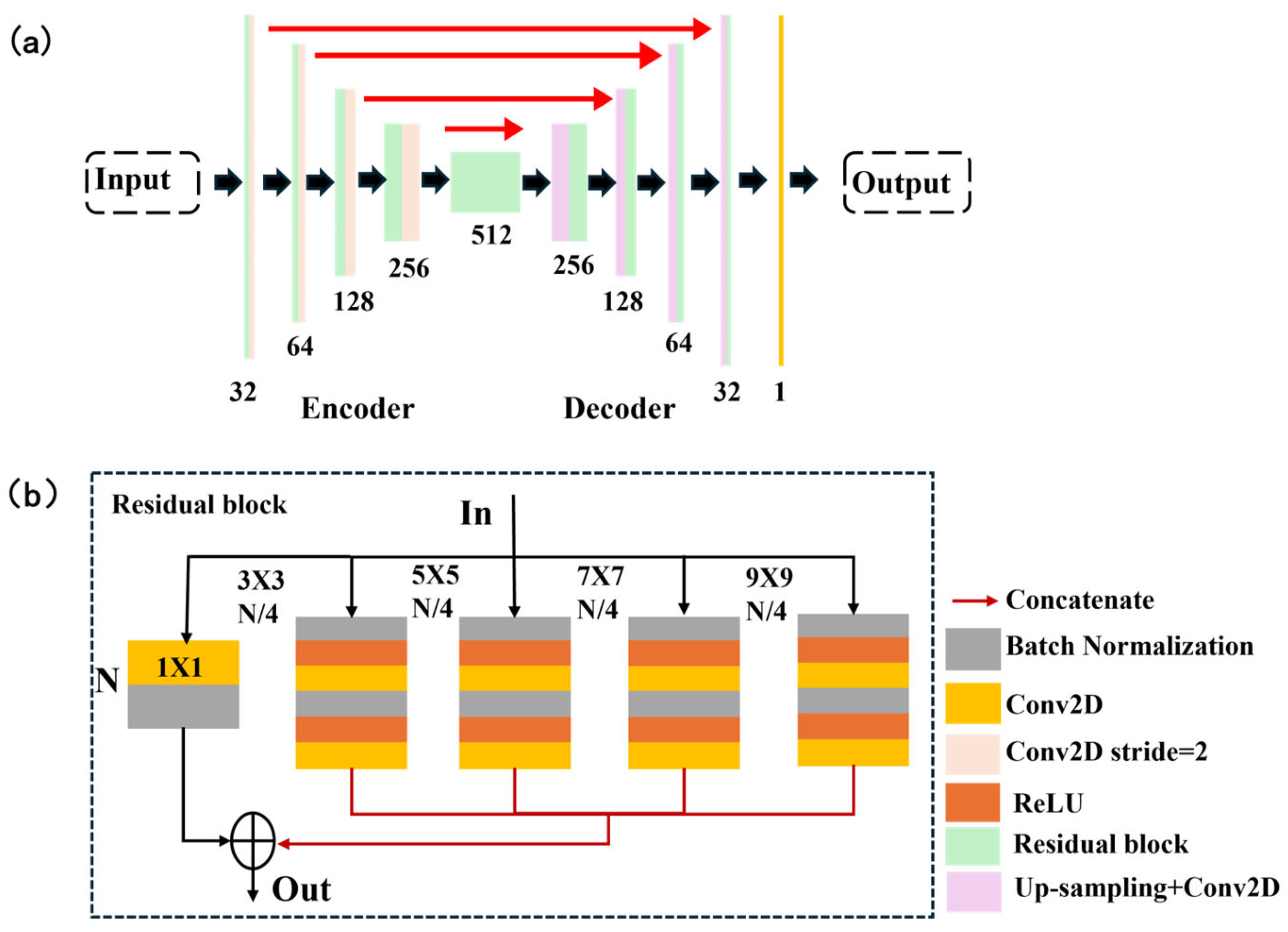In 2020, the team extended their earlier method by employing deep learning to assist SHWFS in wavefront detection [16]. They introduced SH-Net, which can directly predict wavefront distributions from SHWFS patterns while remaining compatible with existing SHWFS systems. The SH-Net architecture is depicted in Figure 5. (a) The pink layer represents downsampling via 3 × 3 convolution with a stride of 2. The red arrow indicates that the downsampling output is connected to the upsampling output. The yellow layer denotes a 1 × 1 convolution with a stride of 1. The numbers below each level indicate the number of channels. (b) Detailed structure diagram of the fragment. N and N/4 denote the number of channels. Each arm is convolved with a different kernel size. For training the network, a total of 46,080 datasets were generated, with 10% allocated for validation. Each dataset consisted of a phase screen as the ground truth and its corresponding SHWFS pattern (256 × 256 in size). The datasets included three different types of phase screens. This approach resulted in a lower root-mean-square (RMS) wavefront error and faster detection speeds. When considering detection speed, SH-Net also outperformed the zonal method and Swanson’s network in terms of accuracy. Direct wavefront detection using SH-Net eliminates the need for centroid positioning, slope measurements, and Zernike coefficient calculations. These advantages make SH-Net a suitable solution for high-precision, high-speed wavefront detection applications.

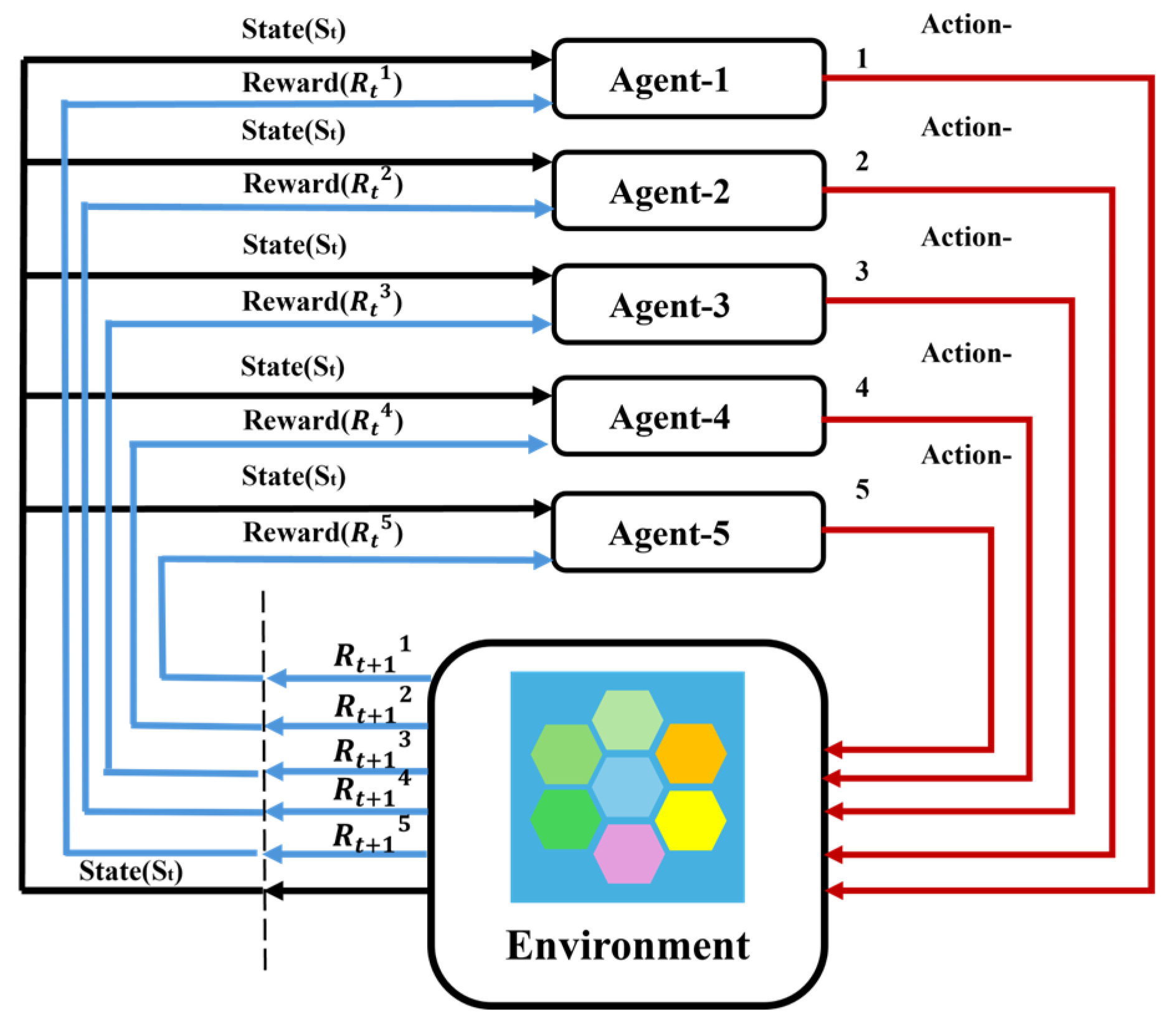
To mitigate the impact of noise, model-free multi-agent reinforcement learning (MARL) can be combined with autoencoder neural networks to implement control strategies. In 2022, Pou et al. [17] introduced a novel formulation of closed-loop adaptive optics control as an MARL problem. Reinforcement Learning (RL) learns a policy function π(s) through trial and error, which maps states to actions and aims to maximize the cumulative sum of rewards (referred to as returns) denoted by J. The goal of finding the optimal policy π∗ can be expressed as identifying the policy that maximizes the expected J:

$${\pi }^{*}=\underset{\pi }{\arg }\max E_{\pi }\left[J\right]=\underset{\pi }{Arg}\max E_{\pi }\left[{\displaystyle \sum _{t=0}^{t=T-1}{\gamma }^t{r}_{t+1}}\right]$$

(3)

where γ is a discount factor weighing future returns, and T is the total time step until the end of the task. This approach maps states to actions while maximizing the expected cumulative returns J. The objective of finding the optimal policy ${\pi }^{*}$ can be expressed as finding the strategy that maximizes J in expectation.

In a system consisting of an SHWFS with 40 × 40 sub-apertures mounted on an 8 m telescope, this solution enhanced the performance of the integrator controller. It served as a data-driven method capable of being trained online without requiring turbulence statistical properties or corresponding parameters. In a fully parallel architecture, the solution time for the combined denoising autoencoder and MARL controller was less than 2 ms.

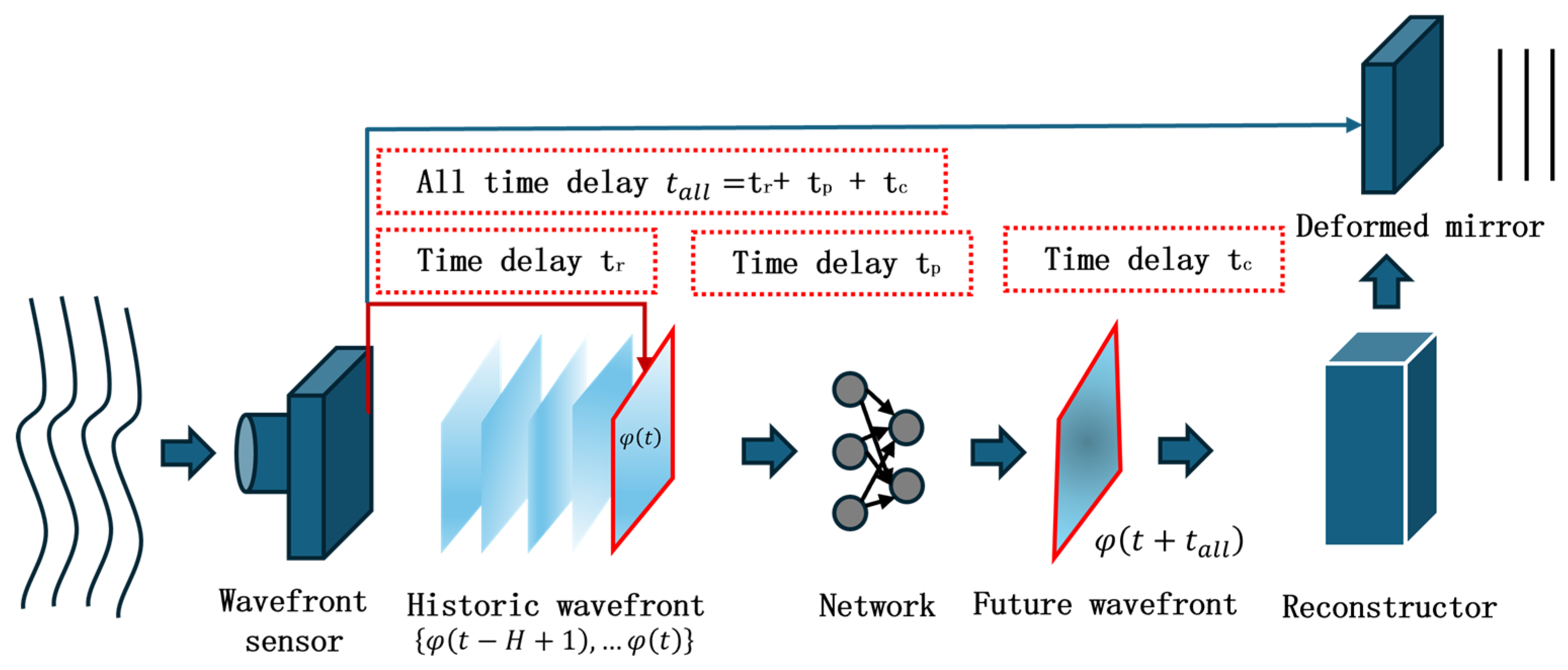
The delay error present in the AO system causes the DM compensation phase to trail behind the actual wavefront aberrations, which limits the performance of the AO system. In 2024, Wang et al. introduced a spatiotemporal prediction network (STP-Net) [18], which takes into account both spatial and temporal correlations of atmospheric turbulence. This network employs feed-forward prediction to mitigate delays in both open- and closed-loop AO control systems.

The STP-Net-based AO system demonstrated smaller correction residuals and a nearly 22.3% improvement in beam quality, providing superior correction performance compared to traditional closed-loop methods. STP-Net operates in real time, achieving predictions at approximately 1.3 ms per frame. The robustness and generalizability of the prediction model could be further enhanced if Hartmann wavefront slope data under varying atmospheric conditions were continuously collected at irregular intervals, and experimental system data were directly integrated into the training set.

Compared to traditional methods, SHWFS wavefront reconstruction based on data-driven techniques offers advantages such as high accuracy, fast speed, and low computational complexity. These benefits have garnered significant attention in the field. To predict turbulence, Guo et al. [19] placed a lenslet array on the telescope’s native image plane and mounted a complementary metal-oxide-semiconductor (CMOS) sensor on its focal plane. This setup enabled the pre-training of a multilayer perceptron (MLP) to project the slope map onto Zernike polynomials, allowing for turbulence predictions 33 ms in advance. Errors detected by the WFS can compromise the accuracy of wavefront reconstruction. To mitigate this issue, Wu et al. [20] used a CNN to map the relationship between the SHWFS sub-aperture light intensity distribution and the corresponding Zernike coefficients up to the 30th order. This approach successfully identified the first 30 Zernike coefficients from light intensity images, even when they contained erroneous points.

Regarding SHWFS digitization, Yang et al. [21] proposed an SHWFS optimization strategy that improved wavefront detection accuracy by four orders of magnitude, reducing Zernike coefficients and wavefront errors in virtual SHWFS. Hu et al. [22] developed a new machine learning-based method for direct SHWFS wavefront aberration detection, capable of estimating the first 36 Zernike coefficients directly from the full SHWFS image within 1.227 ms. Xuelong Li’s team introduced the multi-polarization fusion mutual supervision network (MPF Net) [23], a ghost imaging method that achieved high-quality target image reconstruction through different scattering media using denoising algorithms. Data-driven approaches offer the ability to directly predict wavefront distributions without requiring mathematical modeling or wavefront slope measurements. These methods eliminate the need for slope measurements and Zernike coefficient calculations while delivering lower RMS wavefront errors and faster detection speeds. Furthermore, they remain compatible with existing SHWFS systems. In the era of 30 m-class telescopes, where ultra-high-precision wavefront control is paramount, SHWFS wavefront reconstruction based on data-driven methods will play a crucial role in achieving various scientific goals, including the direct imaging of exoplanets.

2.2. Pyramid Wavefront Sensor (PWFS)

Since Ragazzoni first proposed the concept of PWFS in the 1990s [24], various theoretical studies and numerical simulations have demonstrated that PWFS offers several advantages over the standard SHWFS. These include enhanced and tunable sensitivity, improved signal-to-noise ratio, greater robustness to spatial aliasing, and tunable pupil sampling. Compared to systems equipped with SHWFS, these advantages of PWFS can significantly enhance the closed-loop performance of the AO system.

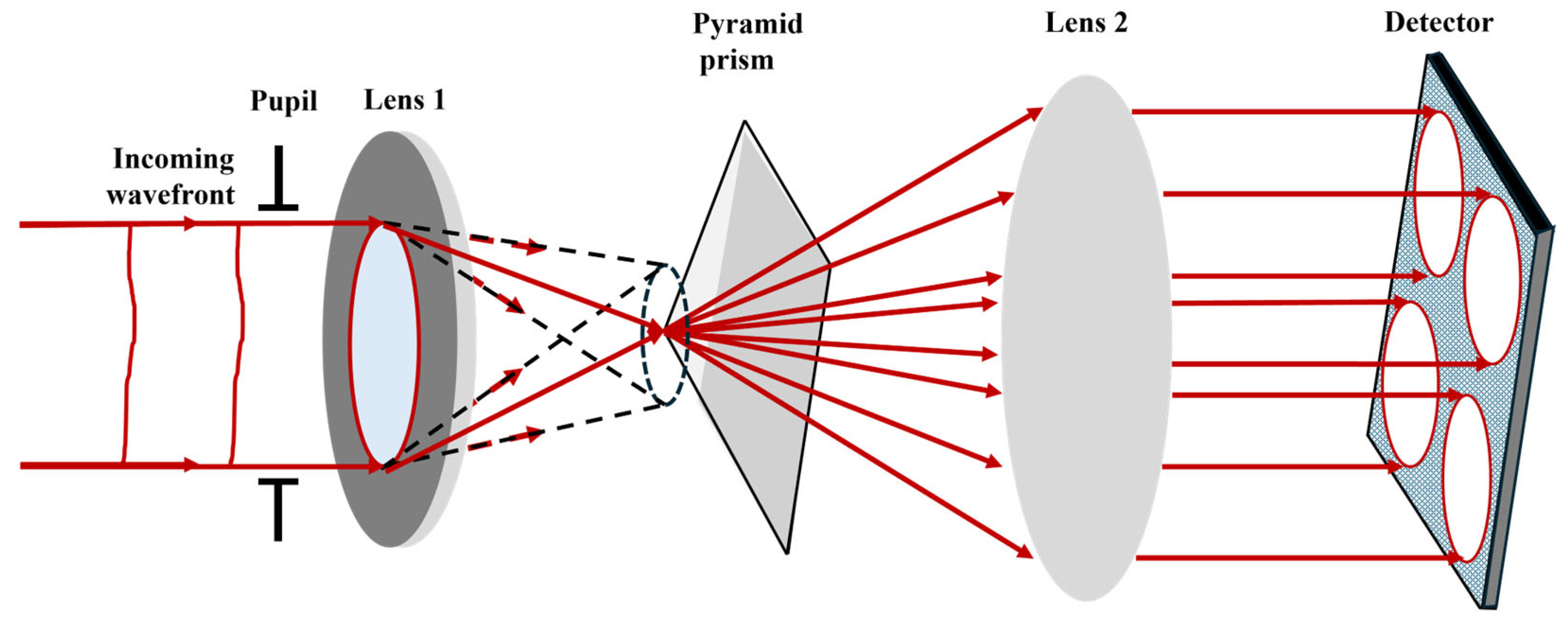
The PWFS is a high-precision wavefront detection device based on amplitude splitting interferometry. Its working principle extends the Foucault knife-edge test [25], reconstructing the entire wavefront morphology by measuring local phase gradients. The core component is a pyramid prism that splits an input beam into four sub-beams. Each sub-beam passes through a lens and converges onto an area detector. By tracking positional shifts of the focused spots, wavefront gradients are calculated, enabling wavefront reconstruction. Figure 6 illustrates the operational principle of PWFS.

Let the prism vertex angle be θ, the incident beam height be h, and the incidence angle be α. According to Snell’s law, the refraction angle β inside/outside the prism satisfies:

$$\sin (\alpha \pm \theta )=n\sin (\beta ),$$

(4)

where n is the refractive index of the prism material.

The optical path difference introduced by the pyramid prism correlates with wavefront tilt. For a horizontal (x-axis) wavefront tilt ϕx, the optical path difference between two adjacent sub-beams is given by:

$$\Delta L=2h\cdot {\varphi }_x,$$

(5)

The corresponding transverse displacement Δx at the focal-plane image point is given by:

$$\Delta x={\displaystyle \frac{\lambda f}{2\pi }}\cdot {\varphi }_x,$$

(6)

where λ is the wavelength and f is the focal length of the lens.

The incident light is focused by the lens onto the vertex of the pyramid prism. The complex amplitudes are as follows:

$${\psi }_{aper}(x,y)=M(x,y)\cdot \exp \left[-i\cdot \Phi (x,y)\right],(x,y)\in {ℝ}^2.$$

(7)

Let Φ: ${ℝ}^2$ → $ℝ$ be the phase screen (in radians) upon entry into the telescope. The complex amplitude corresponding to this phase screen Φ is ${\psi }_{aper}$: ${ℝ}^2$ → $ℂ$. M∶${ℝ}^2$ → $ℝ$ denotes the aperture mask defined as follows:

$$\mathrm{M}(x,y)=\left\{\begin{array}{cc}1,\hfill & (x,y)\in \Omega \hfill \\ 0,\hfill & \mathrm{otherwise},\hfill \end{array}\right\}$$

(8)

where Ω denotes the telescope aperture with a circular central obstruction.

Next, a quadrilateral glass pyramid prism is placed at the Fourier plane of the lens. The prism is described by its phase mask Π. The effect of this phase mask on the focused light is characterized by the Optical Transfer Function (OTF).

$${\mathrm{OTF}}_{\mathrm{pyr}}(\xi ,\eta )=\exp [-i\cdot \prod (\xi ,\eta )],$$

(9)

which introduces certain phase changes according to the prism design.

At the lens’s Fourier plane, a four-sided glass pyramidal prism functions as a phase mask. The influence of this phase mask on the focused light is characterized by the optical transfer function (OTF), which causes phase variations determined by the design of the prism. A second lens then creates an intensity image on the detector.

$${\psi }_{\det }(x,y)={\displaystyle \frac{1}{2\pi }}({\psi }_{aper}\ast PS{F}_{pyr})(x,y),$$

(10)

where $\ast$ is the convolution operator, and the complex amplitude ${\psi }_{\det }$ incident on the detection plane is the convolution of the complex amplitude incident on the detection plane with the PSF of the glass pyramid.

The pyramid PSF is defined as the inverse Fourier transform (IFT) of its OTF.

$$PS{F}_{\mathrm{pyr}}(x,y)=F^{-1}\left\{{\mathrm{OTF}}_{\mathrm{pyr}}(\cdot ,\cdot )\right\}(x,y)$$

(11)

The intensity I(x,y) in the detector plane is then defined as follows:

$$I(x,y)={\psi }_{\det }(x,y)\cdot \overline{{\psi }_{\det }(x,y)}.$$

(12)

In fact, the pyramid’s four facet planes divide the incoming light into four beams, which travel in slightly different directions. Most of the light falling on the detector is concentrated in the four pupil images represented $I^{ij},i,j=\left\{0,1\right\}$. By adjusting the parameters of the second lens, the spatial sampling of optical sub-images can be modified. Within each sub-image Iij, the intensity distribution varies slightly due to differences in the optical paths of each beam. This non-uniformity is utilized as the starting point for recovering wavefront disturbances. Following standard data definitions, two measurement sets s_x and s_y are derived from the four intensity patterns.

$$s_x(x,y)={\displaystyle \frac{[I^{01}(x,y)+I^{00}(x,y)]-[I^{11}(x,y)+I^{10}(x,y)]}{I_0}}$$

(13)

$$s_y(x,y)={\displaystyle \frac{[I^{01}(x,y)+I^{11}(x,y)]-[I^{00}(x,y)+I^{10}(x,y)]}{I_0}}$$

where I₀ is the average intensity per sub-aperture.

$$I_0(x,y)={\displaystyle \frac{I^{00}(x,y)+I^{01}(x,y)+I^{10}(x,y)+I^{11}(x,y)}{4}}$$

(14)

The calibration process establishes a linear relationship between spot displacement and wavefront gradients by utilizing a known wavefront to characterize the system response matrix. These gradient data are subsequently converted into Zernike mode coefficients via the least squares method, enabling full wavefront reconstruction.

PWFS is inherently a nonlinear device. For small wavefront aberrations, it behaves almost linearly; however, its linear range is inversely proportional to its sensitivity. A common method to reduce sensor nonlinearity is to extend the linear range of the PWFS by introducing modulation, although this reduces sensitivity. To enhance sensitivity with an unmodulated PWFS, it is essential to develop nonlinear wavefront reconstruction algorithms that can improve the overall performance of the PWFS. The mathematical description of the wavefront reconstruction problem for PWFS data can be formulated using the wavefront sensing (WFS) equation.

$$s=P\Phi +\eta$$

(15)

where P is the PWFS operator, Φ is the incident (residual) wavefront, s is the sensor data $s=[s_x,s_y]$, and $\eta$ is the noise in the measurements.

Unmodulated PWFSs have a linear range of 1 rad for tip and tilt errors and an even smaller linear range for higher-order modes [26]. Atmospheric turbulence frequently causes wavefront errors that go beyond the linear range of an unmodulated PWFS. The machine learning framework offers a powerful approach for phase reconstruction from wavefront sensor (WFS) data, effectively addressing complex nonlinear relationships between input and output sets. One of the most prominent approaches in this domain is the CNN, which operates under the assumption that features are locally and translationally invariant. This characteristic greatly minimizes the number of free parameters in the model. CNNs rely on training datasets that pair wavefront shapes with their corresponding pyramid sensor data. After training, these algorithms can provide accurate predictions when presented with new data. They are capable of retrieving and inverting potentially nonlinear orthogonal models. Recently, a pioneering effort was made to apply neural networks to the nonlinear wavefront reconstruction of PWFS data [27]. In this research, CNNs were used as reconstructors to broaden the effective dynamic range of Fourier-based WFS into the nonlinear region, where traditional linear reconstructors face substantial performance degradation. In 2020, Landman et al. [28] proposed the use of CNNs for the nonlinear reconstruction of WFS measurements. The phase profile of a DM $\Phi \mathrm{DM}(x,y)$ can be described by a set of modal functions.

$$\Phi \mathrm{DM}(x,y)={\displaystyle \sum _i{c}_i}{f}_i(x,y)$$

(16)

where $c_i$ is the modal coefficient, and estimates are derived from slope measurements from the WFS and denote a set of modal functions.

Actuator modes are employed as the modal basis for wavefront reconstruction. These actuator modes represent the phase profiles elicited when individual actuators on the DM are toggled. The mean squared error is weighted by the square of the RMS of the true modal coefficients to define the following relative loss function:

$$J={\displaystyle \frac{\langle {(c-\stackrel{\wedge }{c})}^2\rangle }{\langle c^2\rangle +\epsilon }}$$

(17)

where ⟨⟩ denotes the average value along the modes and $\stackrel{\wedge }{c}$ represents the predicted modal coefficients. $\epsilon$ prevents the diverging loss of small input RMS. The algorithm is designed to assign equal weight to wavefronts with small RMS values and those with large RMS values.

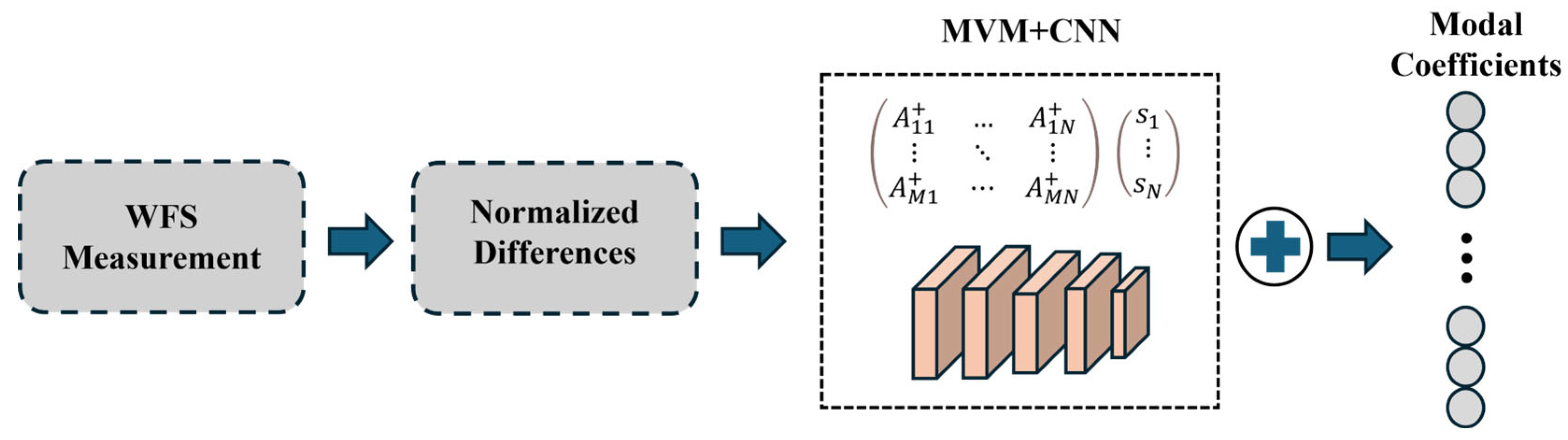
In R. Landman’s scheme, the CNN receives as input the normalized differences observed in both directions, creating a 3D input array with a depth of 2. This array passes through multiple convolutional layers before reaching a final dense layer that outputs the estimated modal coefficients of the wavefront. By using actuator modes as the modal basis, the system takes advantage of the assumptions within the convolutional layers, in contrast to the Zernike basis, which depends on various global features. The system’s DM consists of 32 actuators across the full pupil diameter, with a total of 848 illuminated actuators within the entire pupil. Each actuator has a Gaussian influence function with a standard deviation matching the actuator pitch.

CNN + Matrix Vector Multiplication (MVM) method combines the advantages of CNNs and MVM for wavefront reconstruction. The MVM method estimates the linear term, while the CNN is calibrated to reconstruct only the nonlinear error term:

$$\stackrel{\stackrel{\wedge }{\to }}{c}=A^{+}\overrightarrow{s}+CNN(\overrightarrow{s}).$$

(18)

where it is assumed there is a linear relationship between the measurement vector $\overrightarrow{s}$ and the modal coefficients $\stackrel{\stackrel{\wedge }{\to }}{c}$, and $A^{+}$ is to the regularized inverted interaction matrix.

This scheme demonstrates that nonlinearities can be accurately reconstructed using CNNs. Using CNNs alone as reconstructors under simulated atmospheric turbulence can result in suboptimal closed-loop performance. However, incorporating CNNs as nonlinear correction terms on top of MVM yielded higher Strehl ratios compared to standard MVM methods, particularly when the WFS operated in its nonlinear region. As shown in the scheme in Figure 7, this approach can improve atmospheric aberration estimation. However, nonlinear correction introduces additional computational costs. Measured in floating-point operations (FLOPs), the CNN + MVM method requires approximately 80 megaFLOPs. Astronomical AO systems typically operate at frequencies around 1 kHz. To achieve such speeds, the algorithm requires a computing system with at least 100 GFLOPs of computational power per second, which falls within current computational capabilities. For upcoming extremely large telescopes (ELTs), AO systems are essential for instrument operation, making nonlinear correction critical. Nonlinear errors primarily depend on the number of turbulent elements passing through the pupil. Since ELTs have apertures significantly larger than existing telescopes, both factors exacerbate nonlinear errors and necessitate specialized precision wavefront sensing instruments. Therefore, to enhance the versatility of nonlinear correction schemes, it is necessary to validate the proposed reconstruction method on actual telescopes. This validation must demonstrate the method’s capability to operate under real turbulence conditions and integrate the proposed techniques with precise models for ELT-scale AO instruments.

To further optimize CNNs for nonlinear reconstruction in PWFS, Landman et al. [29] proposed a CNN-based unmodulated PWFS nonlinear reconstructor in 2024. A total of 100,000 phase screens were generated using real on-sky data, with 60%, 15%, and 25% allocated for training, validation, and testing, respectively. For each iteration, the DM voltage was updated using the following equation:

$$D{M}_{t+1}=(1-l)D{M}_t+g{y}_{pred}$$

(19)

where $l$ is the leakage rate of the controller and $g$ is the global gain.

This nonlinear reconstructor exhibited a dynamic range of 600 nm RMS, significantly surpassing the 50 nm RMS dynamic range of classical linear reconstructors. It demonstrated robust closed-loop performance, achieving Strehl ratios greater than 80% at 875 nm under diverse operating conditions. The CNN reconstructor achieves the theoretical sensitivity limit of PWFS, demonstrating that it does not lose sensitivity due to dynamic range limitations. The current computational time of the CNN is 690 µs, with a cycle speed of up to 100 kHz. Future work will further reduce computational complexity to achieve a 2 kHz cycle speed. Unmodulated PWFS operation is feasible under most atmospheric conditions. The next step involves testing the nonlinear reconstructor in real sky conditions.

One of the primary scientific drivers for the development of extremely large optical telescopes is the identification of biosignatures on rocky exoplanets situated within the habitable zones of extrasolar planetary systems. Additionally, predictive control is urgently required to address the system’s inherent lag and the constantly changing atmospheric conditions. Pou et al. [30] proposed an online RL scheme for the predictive control of high-order unmodulated PWFS. This approach integrates offline supervised learning (SL) to train a U-Net architecture designed for nonlinear reconstruction, followed by online RL to train a compact neural network for predictive control. This control method employs a high-order Pyramid Wavefront Sensor (PWFS) to simultaneously drive tilt platforms and high-dimensional mirrors. Under low stellar magnitude conditions, the system demonstrates significantly improved performance and robustness against atmospheric variations. Compared to existing telemetry-based testing methods, this approach calculates atmospheric evolution under the frozen-flow hypothesis, simplifying the predictive control problem for telescopes with spider vane-supported sub-mirrors at 8 m class and larger apertures. One potential challenge arises from petal patterns caused by various factors, which can be mitigated by modifying the modal basis to insert actuators in affected regions. The predictive control strategy is RL-based and currently limited to systems operating at 1 kHz with two-frame latency.

The RL controller’s performance across different loop frequencies primarily depends on AO hardware specifications. Increasing loop frequency inherently leads to more delayed frames and equivalent temporal errors, resulting in comparable performance gains from RL-based predictive control. Selecting optimal loop frequencies for a given stroke becomes increasingly complex for next-generation extreme-AO (ExAO) systems. RL’s adaptability allows automatic compensation for suboptimal operational parameters, offering additional advantages in simplifying AO operations under complex scenarios.

PWFS can be applied to medical imaging for multi-scale retinal imaging to detect microvascular lesions, adaptive optics to correct atmospheric turbulence or optical system aberrations, and industrial inspection for surface defect detection and quality control. Leveraging machine learning and data-driven methods, CNNs in the medical imaging analysis pyramid of retinal images can simultaneously extract vascular textures and optic disc morphology, assisting in diabetic retinopathy diagnosis (accuracy > 95%). In autonomous driving, fusing LiDAR point clouds with camera images enhances obstacle detection robustness. For noise suppression, embedding sensor physical models (e.g., Poisson noise distribution) into network loss functions improves denoising fidelity. When processing pyramid telescope star map data, eliminating atmospheric speckle noise restores stellar position accuracy to sub-pixel levels.

Based on unsupervised and semi-supervised learning, anomaly detection and system self-calibration are achievable. In adaptive optics systems, real-time wavefront aberration calibration reduces mechanical adjustment latency via data-driven feedback loops (response time < 1 ms). The integration of pyramid sensors with machine learning redefines multi-scale perception through data-driven paradigms. Data-driven approaches not only enhance sensor precision and efficiency but also elevate system adaptability and intelligence. Future advancements in algorithm–hardware co-optimization and cross-disciplinary data fusion will enable pyramid sensors to play greater roles in precision manufacturing and environmental monitoring.

2.3. Focal-Plane Wavefront Sensor (FPWFS)

In AO systems, the effects of atmospheric turbulence are counteracted by DMs placed at the telescope’s pupil plane, which rapidly correct the incident wavefront. Modern DMs are equipped with thousands of electrically driven actuators, each capable of applying minute deformations to the mirror surface on millisecond time scales. The effectiveness of this method heavily depends on accurately determining the current state of the wavefront. The current state of the wavefront cannot be fully determined from the focal-plane image alone, as it only provides beam intensity data and lacks the essential phase information needed to characterize the incoming wavefront. Traditionally, AO systems use a separate wavefront sensor (WFS) positioned at a pupil plane, not the imaging plane.

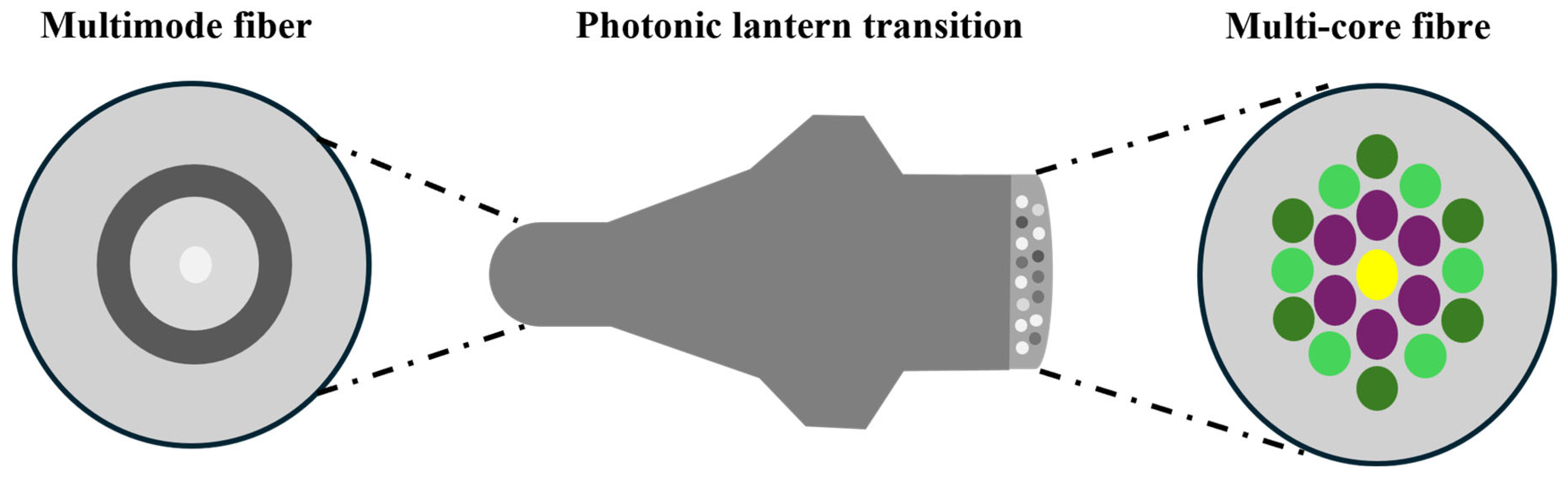
In systems that rely exclusively on pupil-plane WFS, NCPAs can arise between the wavefront observed by the WFS and the wavefront used to create the image, leaving these aberrations uncorrected. Certain aberrations can be especially detrimental to imaging quality. Since a simple image lacks phase information, any inferred wavefront determination is prone to ambiguity. High-contrast imaging instruments are particularly sensitive to wavefront errors, especially NCPAs. FPWFSs address this issue by directly measuring aberrations at the scientific focal plane, making them well-suited for handling NCPAs. Norris et al. proposed a wavefront sensor that combines a photonic lantern (PL) fiber-mode converter with deep learning techniques [31]. This system uses a deep neural network to reconstruct the wavefront, as the relationship between the input phase and the output intensity is nonlinear. The neural network learns the connection between the system’s inputs (wavefront phase) and outputs (the intensity from the single-mode core lantern output). Deep CNNs are adept at learning two types of highly nonlinear relationships: (1) the 2D spatial output amplitude of a multimode fiber (MMF) and (2) the 2D spatial phase/amplitude at the fiber input [32]. The PL is a tapered waveguide that transitions smoothly from a few-mode fiber (FMF) to multiple widely spaced single-mode cores. As shown in Figure 8, the photonic mode converter overcomes several challenges, including the non-constant input–output mode relationship (transfer functions) and the computationally intensive decomposition of mode field images [33]. The PL serves as an interface between the MMF and single-mode fibers, efficiently coupling light from the MMF to a discrete array of single-mode outputs through an adiabatic taper transition. This sensor can be placed in the same focal plane as the scientific image. By measuring the intensity from the single-mode output array, the phase and amplitude of the incident wavefront can be reconstructed without relying on linear approximations or active modulation. This technology also faces limitations. The high power consumption of GPUs makes integration into optical modules challenging, restricting applications in low-power scenarios such as data center interconnects. Experimental validation remains limited to a small number of modes, while practical multi-mode fibers support thousands of modes, and network scalability has yet to be demonstrated. Future efforts should focus on advancing this method from laboratory research to industrial deployment through photoelectric co-design, self-adaptive learning frameworks, and low-cost hardware integration.

Phase retrieval from focal-plane images can lead to sign ambiguity in the even modes of the pupil-plane phase. To overcome this, Quesnel et al. proposed in 2022 a method combining phase diversity from a vortex coronagraph (VC) with advanced deep learning techniques to perform FPWFS efficiently and without losing observing time [34]. They utilized the state-of-the-art CNN EfficientNet-B4 to infer phase aberrations from simulated focal-plane images. The VC, originally introduced by Mawet et al. [35], is a transparent focal-plane mask that scatters on-axis light away from the pupil area. A Lyot stop in a downstream pupil plane blocks the scattered light, allowing for high-contrast observations. Two configurations were considered: SVC and VVC. In the SVC case, a single post-coronagraphic point spread function (PSF) was used, while VVC involved two PSFs obtained by splitting the circular polarization state. The results showed that sign ambiguity was effectively resolved in both configurations, even at low signal-to-noise (S/N) ratios. When trained on datasets with a wide range of wavefront errors and noise levels, the models demonstrated significant robustness. This FPWFS technique ensures a 100% science duty cycle for instruments utilizing VCs and does not require additional hardware for SVC systems. This technology also faces limitations. The training data are designed for a single wavelength. When applied to broadband observations, chromatic aberration effects degrade the consistency of phase diversity, necessitating network re-design. Vortex phase diversity is sensitive to low-order aberrations but exhibits relatively weaker encoding capabilities for high-order aberrations. Simulation results indicate that reconstruction errors significantly increase when the Zernike mode order exceeds 20. Deep learning models require single inferences exceeding 1 ms on CPUs, failing to meet real-time control requirements of adaptive optics systems (typically < 0.1 ms latency). While GPU acceleration improves speed, it raises power consumption and hardware costs. This method provides a novel approach for focal-plane wavefront sensing, yet its practical implementation is constrained by data generalization, hardware precision, noise robustness, and dynamic response capabilities. Embedding physical models, adaptive learning, and edge computing optimization holds promise for advancing this method’s practical deployment in astronomical adaptive optics.

Also in 2022, Min Gu’s team proposed a compact optoelectronic system based on a multilayer diffractive neural network (DN₂) printed on imaging sensors [36], bridging the gap between physical models and data-driven approaches. This system was capable of directly extracting complex pupil phase information from the incident PSF without requiring digital post-processing. The integrated diffractive deep neural network (ID₂N₂), co-integrated with standard complementary metal-oxide-semiconductor imaging sensors, demonstrated the ability to directly extract arbitrary pupil phase information. This innovative approach holds promise as a next-generation compact optoelectronic WFS. However, this kind of network training is based on a single wavelength and a fixed numerical aperture (NA). If the actual system switches the wavelength (such as from visible light to near-infrared) or adjusts the NA (such as replacing the objective lens), the network needs to be retrained, which lacks flexibility.

Traditional wavefront reconstruction methods using focal-plane wavefront sensors infer wavefront phases by analyzing light spot distributions on the focal plane. Incident wavefronts are focused by microlens arrays, forming an array of light spots on the focal plane. Local wavefront gradients are derived by detecting positional shifts of the spots (e.g., centroid displacement). Combined with geometric optics models or iterative algorithms, gradient information is converted into global wavefront phase distributions.

Machine learning and data-driven wavefront reconstruction methods leverage deep neural networks (e.g., fully connected networks, convolutional neural networks) to capture nonlinear relationships between spot displacements and complex wavefront phases, surpassing traditional linear fitting accuracy. By injecting noise into training data, models learn to suppress environmental interference (e.g., CNN models achieve a 30% improvement in signal-to-noise ratio). Reinforcement learning (RL) optimizes parameters such as microlens focal lengths and detector gains, minimizing manual intervention. Transfer learning enables rapid adaptation of laboratory-calibrated models to different sensor configurations or environmental conditions.

The integration of focal-plane wavefront sensors with machine learning enhances precision and efficiency across wavefront reconstruction and anomaly detection, advancing system adaptability and intelligence. Future developments, driven by algorithm-hardware co-optimization and cross-disciplinary data fusion, promise broader applications in medical imaging, astronomical observations, and other fields.

2.4. High-Resolution Imaging Based on Holography

In 1948, Dennis Gabor proposed the concept of holography [37], which records and reconstructs both amplitude and phase information of light waves. This technique offers unique advantages in three-dimensional imaging, optical data storage, and microscopic imaging, while providing a solution for the quantitative description of optical wavefronts. Over seven decades of development, holographic imaging has become a powerful technology for optical wavefront measurement and quantitative phase imaging.

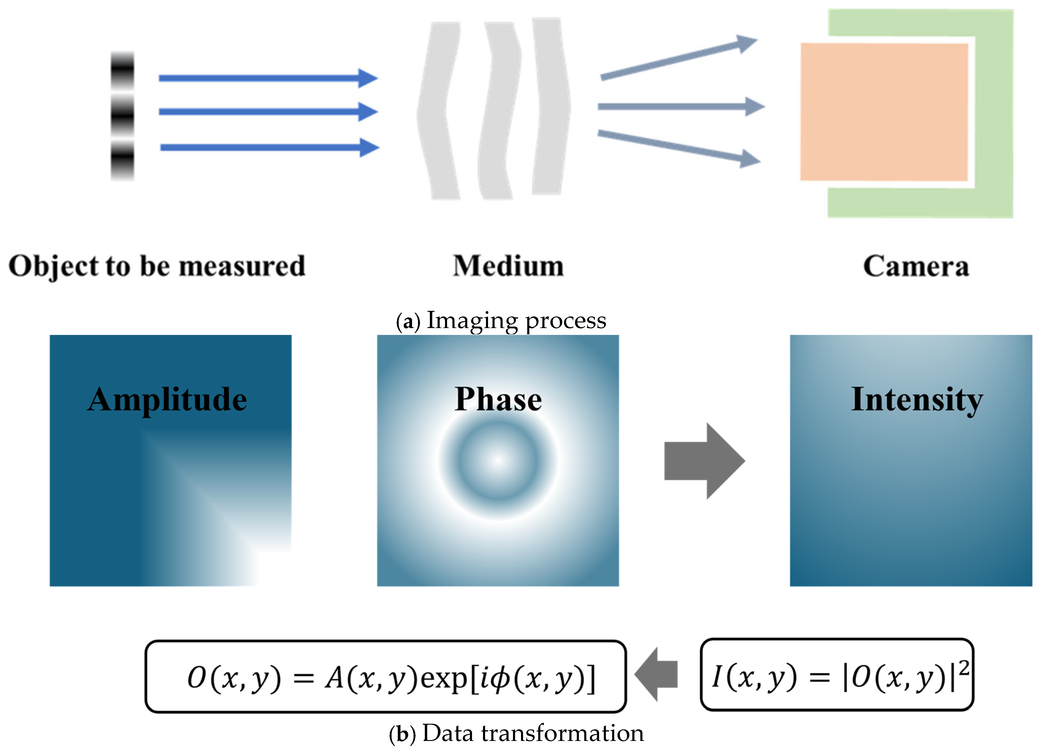
Figure 9 shows the basic methods of holographic imaging. Figure 9a represents the imaging process, and Figure 9b represents the data conversion process. Due to the high-frequency oscillations of visible light, conventional cameras can only record intensity measurements in the spatial domain. Digital holography (DH) employs a reference wave, where the sensor records the interference pattern formed between the reference wave and the unknown object wave. The amplitude and phase of the object wave can then be numerically reconstructed [38]. Based on system configurations, reconstruction methods can be categorized into interferometric and non-interferometric approaches.

Point-source digital inline holographic microscopy (PSDIHM) can generate sub-micron-resolution intensity and amplitude images of objects [39,40]. Quantitative determination of phase shifts is a critical component of digital inline holographic microscopy (DIHM). The simplicity of PSDIHM makes it significant to evaluate its capability for accurately measuring optical path lengths in micrometer-sized objects. Jericho et al. [41] demonstrated through simulated holograms and detailed measurements of diverse micron-scale samples that point-source digital inline holographic microscopy with numerical reconstruction is ideally suited for quantitative phase measurements. It enables precise determination of optical path lengths and extracts refractive index variations with near-0.001 accuracy at sub-micron length scales.

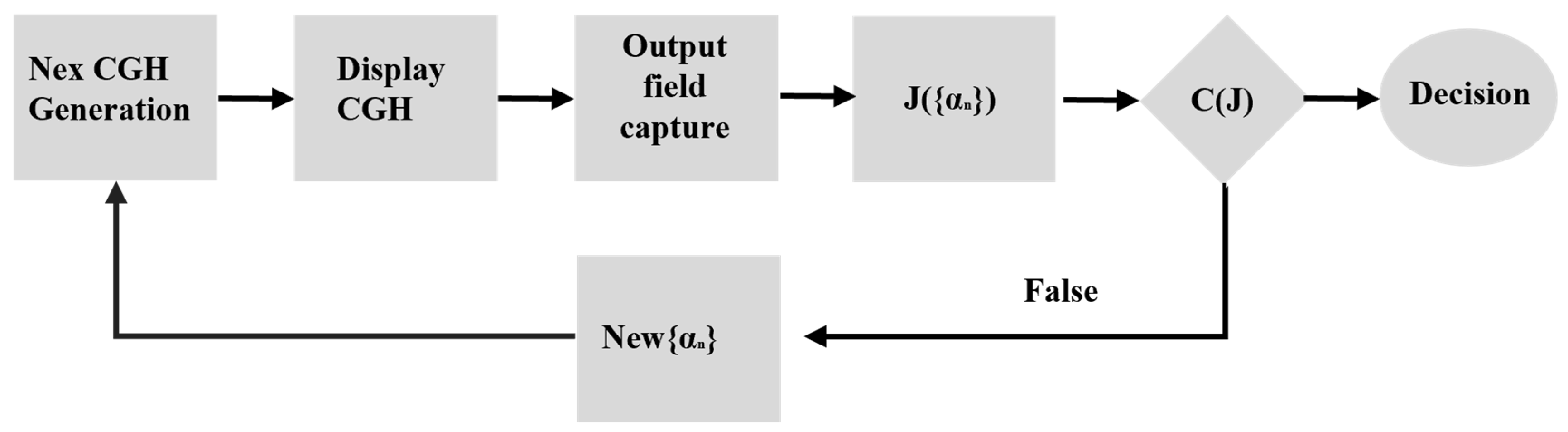
Computer-generated holography (CGH) digitally synthesizes holographic interference patterns that form holograms, diffract incident light, and reconstruct 3D images in free space. CGH involves three key steps: (1) numerical computation of interference patterns between object and reference waves (holograms), (2) mathematical reconstruction and transformation of the generated wavefront, and (3) optical reconstruction using spatial light modulators (SLMs). George Krasin et al. [42] proposed an improved computational Fourier holography method for wavefront aberration measurement. Figure 10 outlines the algorithm workflow for wavefront aberration measurement. First, an initial set of coefficients {αₙ} is used to synthesize a zero-step computational hologram structure. This initializes the iterative algorithm, which selects {αₙ} and computes a temporary wavefront model. The hologram structure is then optimized, implemented on the SLM, and the output intensity distribution is captured by a CCD camera. Peak positions are identified to determine the optimization function value, and the algorithm’s termination conditions are checked. If satisfied, the results are output; otherwise, the process repeats. Experimental results showed that the variation in Δ{αₙ} does not exceed λ/33.

While traditional holographic reconstruction methods are often computationally intensive, modern techniques like Fast Fourier Transform (FFT)-accelerated Fresnel transforms have significantly reduced processing time, enabling near-real-time applications. Conventional holography faces challenges such as high computational complexity, noise sensitivity, and insufficient real-time performance. Recently, the integration of deep learning has introduced new paradigms for holographic algorithm optimization, data reconstruction, and system design, driving intelligent innovation in holographic technologies.

The quality of predicted holograms is inherently limited by dataset quality. In 2022, Shi et al. [43] proposed a new hologram dataset, MITCGH-4K-V2, for directly synthesizing high-quality 3D pure-phase holograms. Their system also corrects visual aberrations through unsupervised training to encode complex holograms. The key innovation lies in retaining the double-phase principle for pure-phase encoding to preserve the advantages of point holography while embedding the encoding process into an end-to-end training pipeline and simplifying CNNs to discover optimal pre-encoding. Supervised training requires pre-existing high-quality labeled phase-only hologram (POH) datasets, limiting training performance and generalization. Unsupervised methods, lacking labeled data, constrain only the reconstructed images, leading to less accurate POH generation. To address this, researchers at Shanghai University proposed a semi-supervised training strategy (SST-holo) for diffraction model-driven neural networks [44], eliminating the need for high-quality labeled datasets. By integrating monocular depth estimation and a Res-MSR module to adaptively learn multi-scale image features, the network’s learning capability is enhanced. A randomized splicing preprocessing strategy (RSPS) preserves original dataset features. Optical experiments validated the semi-supervised approach’s effectiveness in 3D reconstruction and generalization for both monochromatic and color scenarios.

Traditional hologram generation relies on physical models (e.g., angular spectrum method, Fresnel diffraction integrals), which are computationally slow and noise-sensitive. Deep learning enables end-to-end modeling, significantly improving efficiency and robustness. Khan et al. proposed HoloGAN, a generative adversarial network (GAN)-driven hologram synthesis method [45], marking the first use of GANs for holography. It generates high-fidelity 3D holograms 10× faster than iterative methods, enabling real-time holography. Ni et al. developed Holonet [46], a physics-constrained neural network that embeds Fresnel diffraction equations into network layers, achieving 30% lower 3D particle localization errors compared to compressed sensing-based iterative algorithms and a ~5 dB PSNR improvement.

Single-pixel imaging, an emerging computational imaging technique, uses a single nonspatially resolving detector to record images. He et al. proposed a high-resolution incoherent X-ray imaging method combining single-pixel detectors with compressed sensing deep learning [47]. They designed copper (32 × 32 pixels, 150 μm) and gold (64 × 64 pixels, 10 μm) Hadamard matrix masks for high-contrast modulation. Using X-ray diodes to measure total intensity instead of array detectors enhances sensitivity and reduces cost. Leveraging Hadamard matrices’ orthogonality optimizes measurement efficiency, requiring only 18.75% of Nyquist sampling. Noise suppression via wavelet transforms and deep learning improves reconstruction quality for complex structures, achieving breakthroughs in low-cost, low-dose, high-resolution X-ray imaging. Despite challenges in mask fabrication and computational efficiency, this system lays the groundwork for practical single-pixel X-ray cameras.

Researchers combined single-pixel imaging with digital holography to create single-pixel holography. Ren et al. proposed a new computational ghost holography scheme using Laguerre–Gaussian (LG) modes as complex orthogonal bases [48], doubling lateral resolution (vs. random-pattern CGI) and reducing axial positioning errors by 40%, expanding 3D imaging applications.

Phase recovery, a core challenge in computational holography, is addressed by deep learning via data-driven methods, bypassing iterative algorithm limitations. Niknam et al. introduced a holographic light-field recovery method without pre-training data [49], offering new possibilities for data-scarce scenarios. However, sample-wise optimization bottlenecks limit dynamic scene applications. Future directions may include lightweight architectures and automated physical constraint embedding for practicality.

In 2023, Dong et al. integrated CNN-based local feature extraction with vision transformers (ViTs) for global dependency modeling [50], achieving high-fidelity hologram generation with PSNR 42.1 dB and SSIM > 0.95, outperforming CNN-based methods (e.g., Holonet) by ~15%. Future work may focus on ViT’s lightweight design and adaptive physical parameter estimation to reduce hardware requirements.

In 2024, Yao et al. proposed a non-trained neural network DIHM pixel super-resolution method [51]. Their multi-prior physics-enhanced network integrates diverse priors into a non-trained framework, enabling pixel-super-resolved phase reconstruction from a single in-line digital hologram while suppressing noise and twin images. This method avoids data over-reliance and generalization limits of end-to-end approaches, requiring only hologram intensity capture without additional hardware.

Deep learning-enabled holographic displays advance applications in AR and medical imaging. Peng et al. developed a “camera-in-the-loop” training framework [52], achieving hardware-adaptive optimization for holographic models and resolving simulation-to-real transfer challenges. Their differentiable training pipeline, driven by hardware feedback, supports industrial applications sensitive to optical errors. In 2024, Ori Katz et al. proposed image-guided computational holographic wavefront shaping [53], correcting over 190,000 scattering modes using only 25 incoherent compound holograms captured under unknown random illumination. This enables non-invasive high-resolution imaging through highly scattering media without guide stars, SLMs, or prior knowledge, drastically reducing memory usage and avoiding full reflection matrix computation.

Holography enables sub-wavelength resolution, promising applications in astrophysics. Deep learning’s noise suppression and inverse problem-solving capabilities make it a powerful tool for high-resolution imaging. However, challenges remain in data dependency, generalization, computational demands, and real-time processing. Future directions may include quantum neural networks for large-scale holographic acceleration and physics–neural co-design (e.g., embedding Maxwell’s equations into architectures) to enhance generalization across diverse datasets.

2.5. Curvature Sensor

A curvature sensor is a device that infers phase information by measuring the curvature distribution of a light wavefront. It is widely used in adaptive optics (AO), retinal imaging, laser processing, and other fields. Traditional curvature sensors rely on physical models and numerical optimization algorithms, but their limitations—such as noise sensitivity, high computational complexity, and restricted dynamic range—hinder performance in complex scenarios. Recently, the rapid advancement of machine learning (ML), particularly deep learning (DL), has opened new technical pathways for optimizing and innovating curvature sensors.

The core principle of curvature sensing involves measuring intensity differences between two conjugate planes (e.g., the focal plane and a defocused plane) to reconstruct wavefront curvature. Its mathematical model is based on the Fresnel diffraction integral, simplified as follows:

$$\Delta I(x,y)\propto \varphi ″(x,y)\cdot \Delta z,$$

(20)

where $\varphi ″(x,y)$ represents the second derivative of the wavefront (curvature), $\Delta z$ is the distance between the planes, and $\varphi ″(x,y)$ is the measured intensity difference.

Traditional phase recovery methods face limitations: Noise (e.g., shot noise, thermal noise) causes curvature estimation errors; large phase distortions invalidate the Fresnel model, requiring iterative algorithms with high computational costs; and phase recovery often assumes wavefront sparsity or smoothness, limiting applicability.

Machine learning addresses these challenges by directly extracting features from intensity images and predicting wavefront information, significantly enhancing robustness and efficiency. For example:

• In 2022, Zhu et al. proposed a fiber curvature sensor combining coreless and hollow-core fibers with ML [54], achieving high sensitivity (16.34 dB/m⁻¹) and a large dynamic range (0.55–3.87 m⁻¹). This demonstrated ML’s potential for intelligent fiber sensing systems.
• Li et al. integrated fiber speckle pattern analysis with CNN regression [55], achieving 94.7% prediction accuracy, with minimal RMSE (0.135 m⁻¹).
• In 2023, Deleau et al. applied neural networks to long-period grating (LPG) distributed curvature sensing [56], combining high-sensitivity optics with data-driven methods. Their model maintained 0.80% median error under noise, showing robustness to signal distortion.
• In 2024, Pamukti et al. developed a Mach–Zehnder interferometer (MZI) and random convolution kernel (RaCK)-DNN method [57], achieving 99.82% classification accuracy and RMSE of 0.042 m⁻¹ in regression tasks, excelling in low-curvature ranges (0.1–0.4 m⁻¹) for landslide monitoring.

Key advantages of ML-driven curvature sensors include noise suppression, handling high-order aberrations, and real-time control. However, challenges remain in data dependency, model generalization, and physical interpretability. Future directions may involve hybrid models, lightweight algorithms, and interdisciplinary fusion (e.g., multi-modal data integration). These advancements could revolutionize applications in astronomy, biomedical imaging, and precision manufacturing, driving breakthroughs in optical technology.

3. System Aberration Control

Due to “imperfect” physical devices and “suboptimal” experimental environments, optical systems inevitably experience wavefront aberrations, which significantly degrade the quality of the optical field. To address this issue, researchers have developed various wavefront correction techniques that are extensively applied in astronomical observation, optical communication, microscopic imaging, and holography. However, wavefront correction techniques that rely on WFS are unsuitable for environments with strong interference, as they tend to be expensive and require complex system architectures. WFS-less calibration techniques are often less effective, as they can become trapped in local optima and involve time-consuming iterative processes.

3.1. Piston Detection

Optical sparse aperture systems, such as segmented mirror telescopes and telescope arrays, provide large overall apertures with high resolution at reduced cost and weight. Among the factors affecting imaging quality, piston aberration along the optical axis (z-axis) and tilt along the x-axis and y-axis of the sub-mirrors relative to a reference sub-mirror have the most significant impact. To achieve imaging quality close to the diffraction limit, segmented telescopes must maintain extremely high co-phase accuracy of their sub-mirrors [58]. To achieve optimal imaging performance, it is crucial to maintain the optical path length between sub-apertures (pistons) within a small fraction of a wavelength. Failing to do so results in a significant degradation of imaging resolution.

Accurate co-phasing of sub-mirrors involves two main steps: (1) sub-mirror co-phase error detection and (2) sub-mirror error correction, which can be implemented using a multi-dimensional precision displacement platform. Based on these principles, co-phase error detection methods can be categorized into two groups: (1) pupil surface detection methods using specific hardware sensors [59] and (2) focal-plane image-based methods, which analyze image information [60]. In 2016, Jiang et al. [61] identified a clear mathematical relationship between the modulation transfer function (MTF) of a system’s OTF and the piston error of sub-mirrors for point-source observation targets under broadband illumination. This theoretical relationship was fitted to a piecewise quartic polynomial function. Their method achieved a detection range extending up to half the coherent wavelength of the input broadband light, with a detection accuracy of 0.026λ RMS (λ = 633 nm). However, this approach only measures the absolute piston error between sub-mirrors and does not provide information about the specific relative spatial positions of each sub-mirror.

The generalized pupil function (GPF) of a segmented telescope is given by:

$$P(\epsilon ,\eta )={\displaystyle \sum _{n=1}^N{p}_n}(\epsilon ,\eta )\exp \left[i{\displaystyle \frac{2\pi }{\lambda }}(e_n{Z}_1+t_{xn}{Z}_2+t_{yn}{Z}_3)\right]$$

(21)

where $Z_1$, $Z_2$, and $Z_3$ are the first three terms of the Zernike polynomial; $e_n$, $t_{xn}$, and $t_{yn}$ are the corresponding Zernike polynomial coefficients of the nth sub-mirror; $(\epsilon ,\eta )$ is the coordinate vector at the pupil plane; $p_n$ is the binary function of the sub-aperture; and N is the total number of sub-mirrors.

In recent years, advancements in deep learning have enabled state-of-the-art CNNs to estimate wavefronts represented by Zernike coefficients directly from the intensity image of a point source as well as from the intensity image of a specified extended object. Li et al. [62] utilized multiple pairs of focal and defocused images at four different wavelengths to train a shallow neural network. Their method successfully reduced the piston error range from [0, 10λ] to [0, λ]. Mei et al. [63] proposed a CNN-based piston detection method that achieved an accuracy of 0.062λ, although the capture range of this method was limited to [0, λ]. Phase calibration methods have also adopted deeper networks to further enhance the accuracy of piston detection.

Guerra-Ramos et al. [64] applied a CNN for detecting local pistons between segments of a segmented mirror. This method accurately measured the piston step values between segments and achieved a wide capture range at visible wavelengths. By using intensity measurements at visible wavelengths, the detector could be positioned at a single defocused plane. The network architecture is shown in Figure 11. The CNN was trained in a fully supervised fashion. This approach required only a visible-light imaging camera, with minimal or no additional equipment, and showed robustness to variations in the Fried parameter of the atmosphere. Fried is a key parameter to measure the effect of atmospheric turbulence on optical imaging and represents the effective length of phase coherence during the propagation of light waves in the atmosphere. Using a combination of wavelengths, the approach achieved a wide capture range with an accuracy of approximately ±0.0087λ0. This highlights its potential for precise piston detection while maintaining practical applicability in various atmospheric conditions.

To explore the further streamlining of the detection process, Ma et al. [65] proposed a piston detection method using broadband extended images with a single deep convolutional neural network (DCNN). Broadband images, both focused and defocused, were utilized to calculate feature vectors, which served as inputs for training the DCNN, with the corresponding pistons as the outputs. This method is notable for its ability to perform precise phasing, achieve high sensing accuracy, and maintain a broad capture range without the need for combined wavelengths. With a broadband of 100 nm, the method achieves a capture range of 10λ in the longest unit. In terms of detection accuracy, it provides an average RMSE of 12 nm for a three-aperture imaging system and 32 nm for a six-aperture imaging system, enabling fine phasing without relying on additional methods.

SL-based methods for identifying co-phase errors in segmented mirrors often struggle to achieve high accuracy in practical applications due to discrepancies between the training model and the actual system. RL algorithms [66], in contrast, do not require system modeling during operations. In 2020, Guerra-Ramos et al. [67] applied RL to correct piston misalignment between segments in segmented mirror reflecting telescopes. Due to its narrow capture range and rapid agent learning, this approach was effective for piston fine-tuning to maximize the Strehl ratio of the wavefront. Building on this foundation, Li et al. [68] proposed a method for the automatic correction of piston errors in segmented mirrors based on deep RL. A mask was positioned at the pupil plane of the segmented telescope optical system, with deep learning applied to extract low-dimensional features from high-dimensional data. Reinforcement learning (RL) employed the Markov decision process to make decisions. Through ongoing interaction with the external environment, deep RL algorithms learned to execute appropriate actions in complex scenarios. The long-term reward for the RL agent is defined by the following equation:

$$G_t=R_t+\gamma \cdot R_{t+1}+{\gamma }^2\cdot R_{t+2}+{\gamma }^3\cdot R_{t+3}\cdot \cdot \cdot \cdot \cdot \cdot$$

(22)

where $\gamma$ is the discount factor and $R_t$ is the reward function value obtained by the agent at time step t.

The RL algorithm is illustrated in Figure 12, where the focal-plane image of the optical system, after introducing a multi-hole mask, serves as the environmental observation variable. The segmented telescope acts as the interaction environment for the agent. And schematic diagram of the automatic correction of sub-mirror piston error is shown in Figure 13. Based on the input focal-plane image, the agent directly outputs the piston error correction for each sub-mirror. After the sub-mirror correction, the re-inputted focal-plane image allows the agent to output the next correction quantity for each sub-mirror, facilitating iterative improvements.

This method enables the automatic co-phasing of piston errors among multiple sub-mirrors in segmented mirror telescopes. The piston error correction range can be extended by up to 10 wavelengths. Using a trained deep RL algorithm, piston co-phase errors were automatically corrected to less than λ/20 (RMS) root-mean-square within the 10-wavelength range for each of the six sub-mirrors in the segmented system.

The dataset used for this approach holds significant implications for piston detection, particularly in achieving both high precision and large-scale detection. In 2022, Zhao Weirui and colleagues [69] proposed a high-precision piston detection method with a large capture range based on the coordination of multiple neural networks. A specialized dataset was created by placing a mask with a sparse multi-sub-pupil configuration at the conjugate plane of the segmented mirror, making it highly sensitive to pistons. Two types of neural networks were constructed for different detection stages: (1) Coarse Detection Network (CDnet), which identifies large piston errors and brings them within the effective detection range of the Fine Detection Network (FDnet); (2) Fine Detection Network (FDnet), which performs high-precision piston detection after CDnet has reduced the error to a manageable range. Through iterative coordination between the two networks and the correction actuator, the method effectively balances the trade-off between detection range and precision. It also offers advantages such as datasets optimized for feature extraction, high detection precision, and fast detection speeds. In 2023, Yue et al. [70] addressed the difficulty and complexity of piston error detection in segmented telescopes by proposing a hybrid artificial neural network method. The ResNet architecture was first employed to learn the mapping between focal-plane degradation images and the signs of piston error, while a BP neural network was used to learn the relationship between the MTF and the absolute value of the piston error. After training, the hybrid network could detect sub-mirror piston errors with high precision and across a wide range. The detection range extended up to the entire coherent length of the input broadband light, with a detection accuracy reaching 10 nm. For optical sparse aperture systems, segmented pistons are introduced to improve the observation capabilities of segmented telescopes. Data-driven methods, such as those discussed, enable rapid piston detection and correction for atmospheric turbulence without requiring additional hardware. These approaches offer notable benefits, such as high detection precision, an extended detection range, reduced hardware costs, compact network structures, and ease of training. As a result, they have profound implications for further enhancing the observation capabilities of survey telescopes.

3.2. Aberration Suppression

Wavefront aberrations can be corrected using either a DM or a spatial light modulator (SLM). To generate the necessary control signal for the DM or SLM, optimization techniques can be utilized. However, this method involves finding the optimal control signal through stochastic, local, or global search algorithms, which is time-intensive due to the numerous iterations and measurements required. Alternatively, WFS techniques can address wavefront distortions by using a wavefront sensor (e.g., Shack–Hartmann wavefront sensor) to direct the control signal for the DM or SLM. However, this approach is often limited by the need for expensive optical components, multiple measurements, and complex calibration procedures.

Simultaneously measuring aberrations at different spatial locations using single-frame data is essential for achieving wide-field AO. In 2021, Zhao et al. proposed a WFS method based on deep learning [71]. Figure 14 shows the basic scheme for deep learning wavefront aberration correction. This trained neural network directly restored wavefront aberration phases from distorted intensity images and performed corrections using a phase-type SLM. After correction, the standard deviation of the wavefront phase was reduced to one-fourth of its initial value, and the maximum value of the focus spot of the convex lens increased by a factor of 2.5. The correction was demonstrated to be both effective and feasible in real atmospheric turbulence environments. Studies have shown that deep learning techniques are fully capable of replacing conventional WFS as an effective method for improving and optimizing AO systems.

There is a growing need to develop low-cost, high-speed solutions to preserve image quality during observations with wide-field survey telescopes. In 2022, Wu et al. [72] proposed a machine-learning-based alignment metrology system using stellar images captured by the scientific camera. The network architecture is illustrated in Figure 15. Each hidden layer contains 300 nodes, the input layer comprises 30 nodes corresponding to low-order Zernike polynomial coefficients, and the output layer includes 8 nodes for bias parameters. After two-step active alignment, the eccentricity position error is less than 5 μm, and the tip-tilt positional error is below 5″ (arcseconds) in over 90% of cases.

Figure 16 shows a schematic diagram of the turbulence prediction and correction model of the AO system based on deep learning. For turbulence, the key lies in identifying the flow direction. Schwarz et al. leveraged the fractal persistence of wavefronts based on the fractal characteristics of fractional Brownian motion [73], employing statistical correlation to optimize prediction models, offering an effective solution for turbulence compensation. Poyneer et al. provided a theoretical framework and practical approach for real-time compensation of complex atmospheric turbulence through effective decomposition of Fourier modes and precise prediction using Kalman filters [74]. Figure 15 illustrates a turbulence prediction and correction model for AO systems based on deep learning. To address the challenge of accurately predicting stochastic turbulence, Wu et al. [75] also proposed a neural network model based on LSTM in 2022. This neural network was combined with a turbulence correction time-series model, enabling accurate and stable real-time AO corrections. In 2023, Wu et al. [76] introduced a holographic-diffuser-based wavefront sensor (HD-WFS) for the unambiguous retrieval of multiplexed wavefront information. This method exploited the local orthogonality of speckles generated by holographic diffusers to perform simultaneous measurements of wavefront information at multiple spatial locations.

Adaptive optics is widely used in microscopy to correct aberrations through reconfigurable elements. In 2023, Cai et al. modified a traditional inverted fluorescence microscope by adding a 4f relay system [77] at its camera port and dynamically controlling the pupil function via a spatial light modulator (SLM). Positioned at the Fourier plane, the SLM loaded encoded patterns to modulate the effective pupil shape in real time, enabling flexible control over incident light fields. Extending the Fourier slice theorem from conventional computed tomography (CT) to incoherent tomography, they proposed a novel model where pupil modulation equivalently performs spectral slicing. Through optical transfer function (OTF) analysis, they designed a hybrid modulation scheme combining non-centrosymmetric annular and circular apertures, achieving high-resolution 3D reconstruction via phase retrieval and back-projection algorithms. By deeply integrating hardware programmability with software algorithm innovation, PALFM (Pupil-Modulated Axial Light-Field Microscopy) revolutionized incoherent tomography, offering high resolution, motion-artifact-free imaging, and strong adaptability. This cost-effective 3D microscopy tool demonstrates significant potential for biomedical research. Hu et al. [78] proposed a physics-based machine-learning-assisted MLAO method for versatile and fast aberration correction. This method could be applied across various microscope modalities, offering robustness and operability even under low signal-to-noise ratio conditions. In 2024, Long et al. [79] advanced the data-driven approach by proposing a wavefront correction scheme based on a Zernike-fitting neural network (ZFNN) and a vortex beam generation model. By integrating deep learning techniques into WFS-less calibration and using a vortex beam field sensitive to phase perturbations as a probe beam, this scheme achieved fast calibration while addressing the convergence issues associated with local optima.

For the new generation of sky survey telescopes, data-driven methods adequately meet the requirements for aberration correction, providing key insights for achieving high-speed, wide-field aberration correction. These approaches enable fast and accurate wavefront reconstruction while offering advantages such as single-measurement capability, simplified optical paths, and broad versatility. In the future, further optimization of code execution speed, the development of faster gradient extraction algorithms, and the integration of efficient gradient-based algorithms will likely enable wavefront reconstruction durations to remain within tens of milliseconds, ensuring rapid and accurate aberration correction.

3.3. Intelligent Focusing Element

The core of intelligent focusing lies in the synergistic optimization of hardware and algorithms. Future advancements in AI and novel optical materials will drive faster, adaptive, and miniaturized focusing technologies. Innovations such as Liquid Lenses, Metalenses, and Bimorph Mirrors are rapidly evolving in the field of intelligent focusing, addressing demands for programmability, miniaturization, and enhanced performance.

(1)

Liquid Lens

A liquid lens is a novel optical device that dynamically adjusts focus through liquid–liquid or liquid–gas interface deformation or electrowetting effects. It offers advantages such as compact structure, rapid response, and the absence of mechanical moving parts, making it promising for applications in micro-imaging systems, adaptive optics, and biomedical detection. Recent breakthroughs in material systems, actuation mechanisms, and integration technologies have significantly advanced this field.

The core principle of liquid lenses involves modulating the curvature of liquid–liquid or liquid–gas interfaces via external stimuli (e.g., electric fields, pressure, temperature, or light) to adjust focal length. Early research focused on electrowetting effects. In 2000, Berge’s team first proposed a liquid lens based on electrowetting principles, achieving zoom control by adjusting the contact angle between conductive and insulating liquids using voltage [80]. In recent years, dielectrophoretically driven dual-liquid lenses have gained attention for their low power consumption and high stability. For example, in 2018, Li et al. developed a replaceable and focus-tunable electrowetting optofluidic lens [81]. This lens comprises an annular chamber and a central chamber. Conductive liquid is injected into the bottom of both chambers, while the rest of the chamber is filled with silicone oil. Multiple apertures connect the two chambers, forming a closed-loop fluidic system. The liquid–liquid interface (L-L interface) can be manipulated via applied voltage to achieve dynamic focusing. The relationship between the contact angle θ and the applied voltage U can be described as follows:

$$\cos \theta ={\displaystyle \frac{{\gamma }_1-{\gamma }_2}{{\gamma }_{12}}}+{\displaystyle \frac{\epsilon }{2{\gamma }_{12}d}}{U}^2,$$

(23)

where $\epsilon$ is the dielectric constant of the insulating layer, $d$ is the thickness of the insulating layer, and ${\gamma }_1$ and ${\gamma }_2$ are the interfacial tensions of the hydrophobic layer/silicone oil and the hydrophobic layer/conductive liquid, respectively.

Figure 17 shows the cross-sectional structure and working principle. Under the equilibrium state, applying a voltage U1 decreases the contact angle θ1, thereby altering R1. This change causes capillary pressure to pull the conductive fluid upward, resulting in variations in h1 and h2. By altering the position of the L-L interface, precise control over the object and image distances can be achieved, enabling the desired magnification. The optofluidic lens adjusts focus by deforming the L-L interface. This single lens can serve as a zoom lens, offering a compact and user-friendly solution. The lens has a maximum displaceable distance of approximately 8.3 mm and a zooming ratio of ~1.31×. This combination of translational motion and focal length stability makes it a versatile optical component suitable for a wide range of applications.

To further optimize liquid lenses, in 2019, Tang et al. proposed an electrowetting liquid lens with a dual-aperture [82], using a liquid crystal (LC) cell and a polarizer to achieve the switching between the internal and external channels. In 2022, Wang Danyang et al. designed and fabricated a focusable and tunable liquid cylindrical lens based on electrowetting [83], which expanded the focal length of the liquid cylindrical lens. In 2022, researchers from Hefei University of Technology developed an adaptive liquid lens using a novel transparent electro-responsive fluid, dibutyl adipate (DBA) [84]. The new electro-responsive liquid enables the lens to be small in size, light in weight, and easily fabricated. In 2023, Xu Jinbo et al. proposed a three-phase (air, conductive liquid, and dyed insulating liquid) electrowetting liquid lens (TELL-DLI) with a deformable liquid aperture [85]. The focal length varies from −451.9 mm to −107.9 mm and can be switched among circular, elliptical, fan-shaped, and strip shapes. In 2024, Yin et al. proposed a field of view (FOV) tunable liquid lens driven by the electrowetting effect [86]. This lens can achieve focal length adjustment and FOV deflection by applying voltages to the four sidewall electrodes, featuring a simple structure and miniaturized actuation. In 2025, Li et al. developed the first real-time holographic camera through a synergistic design of liquid lens hardware innovation and deep learning algorithm optimization [87]. Leveraging a voice coil motor-driven elastic membrane liquid lens, the system adjusts lens curvature by applying electrical current, achieving focal switching within 15 ms. The FS-Net holographic generation network takes focused stacks (Focus Stack) of real 3D scenes as input and outputs RGB–channel complex amplitude holograms. This breakthrough enables high-speed capture and high-fidelity holographic reconstruction of real 3D scenes, opening new avenues for holographic applications in 3D display and metrology.

Despite rapid advancements in liquid lens technology, challenges remain in long-term stability, environmental sensitivity (e.g., temperature variations), and optical aberrations (e.g., chromatic aberration in polychromatic light). Interface behavior becomes uncontrollable under extreme temperatures or pressures. Future research may focus on optimizing lens structures and drive strategies using machine learning.

(2)

Metalenses

Metalenses are planar optical devices based on metasurfaces, which manipulate light waves’ phase, amplitude, and polarization through sub-wavelength-scale artificial structures to achieve functions such as focusing and imaging traditionally performed by conventional lenses. Their core advantages include ultrathin designs, easy integration, multifunctionality, and the potential to overcome the diffraction limit.

Early metalenses faced limitations in bandwidth and chromatic aberrations. In 2016, Capasso’s team proposed a design combining geometric and propagation phases, achieving broadband achromatic metalenses in the visible spectrum [88]. Stanford University’s Arbabi team developed multi-layered meta-atom designs, enabling high-efficiency, large-numerical-aperture (NA) metalenses [89]. Aaron et al. integrated liquid crystals with metasurfaces to create electrically tunable focal-length metalenses [90]. Shrestha et al. first controlled both group delay and phase delay in dielectric metalenses, breaking single-wavelength operational constraints [91]. Metalenses have since been applied in smartphone camera modules and AR/VR near-eye displays [92], with roll-to-roll nanoimprint lithography enabling low-cost, large-area fabrication.

While metalenses have transitioned from fundamental research to industrialization, challenges remain in dynamic tuning, material reliability, and scalable manufacturing, where precision must be balanced with cost [93]. Despite their compactness, trade-offs often exist between throughput, efficiency, and scalability—especially for large-aperture systems—limiting their practicality.

(3)

Bimorph Mirrors

Bimorph mirrors are adaptive optics components driven by piezoelectric materials, where electric fields adjust mirror curvature to correct wavefront aberrations. Applications span astronomy, laser beam shaping, and biomedical imaging. Recent advances in materials science, control algorithms, and precision manufacturing have expanded their performance and applications.

Traditional monolithic piezoelectric deformable mirrors faced limitations. Rodrigues et al. proposed a modular bimorph deformable mirror design [94], enhancing performance through modular architectures for adaptive optics systems. In 2019, Alcock et al. integrated multi-layer piezoceramics with thin mirror plates [95] to achieve nanoscale deformations under electric fields, enabling sub-millisecond dynamic correction for X-ray optics requiring high-precision wavefront control.

The performance of bimorph mirrors heavily depends on closed-loop control algorithms. Recent research has shifted from traditional Zernike mode decomposition to data-driven adaptive control. Gautam et al. combined neural networks (NNs) and Gaussian process regression (GPR) to map mirror deformations to voltage inputs [96], reducing root mean square error (RMSE) by 68% compared to physical models and optimizing X-ray focal spots from 2.1 μm (open-loop) to 0.8 μm. Zhang et al. proposed a controller based on a tandem neural network to optimize the dynamic performance of X-ray double-crystal mirrors [97]. By implementing a tandem structure for multi-band cooperative control, this hierarchical neural network design balances precision and efficiency, providing a novel paradigm for the intelligent control of precision optical devices and driving the intelligent upgrade of X-ray optical systems.

Despite these advances, challenges persist in piezoelectric hysteresis, large-scale fabrication, and cost. Hybrid designs (e.g., combining voice coil motors) partially address hysteresis, while additive manufacturing offers pathways for lightweight, low-cost devices.

4. Conclusions and Outlook

Compared to conventional wavefront reconstruction methods, data-driven, high-resolution imaging techniques offer the ability to establish nonlinear correspondences between image intensity information and wavefront phase. These methods also enable rapid wavefront estimations without the need for dedicated hardware. By coordinating multiple neural networks, it is possible to balance detection range and accuracy effectively, while creating datasets optimized for easy feature extraction. These methods exhibit high detection accuracy, fast detection speed, and robustness against changes in atmospheric conditions, such as variations in the Fried parameter. Additional advantages include simple application conditions, independence from customized sensors, and high computational efficiency. Moreover, these techniques offer a wide capture range, making them ideal for applications requiring both precision and speed. In

Table 2. Comparison of different methods applicable to wavefront reconstruction.

Method	Advantage	Disadvantage
Interaction Matrix-Based Approach	1. Mature and widely used; 2. High flexibility.	1. High computational complexity; 2. Reliance on calibration data.
Fourier analysis method	1. High computing efficiency; 2. Segmented pupil.	1. Relies on a linear approximation model; 2. Large modulation amplitude is required.
Hilbert transform method	1. Calculation speed is fast; 2. High boundary accuracy.	1. Only applicable to non-modulated sensors; 2. Sensitive to noise and limited aperture.
Linear iterative method	1. Medium complexity; 2. High adaptability.	1. Limited effect on high nonlinear residual; 2. Multiple iterations may be required.
Nonlinear iterative method	1. Nonlinear response; 2. The performance is better than the linear method.	1. Computational complexity is extremely high; 2. Need accurate modeling.
Machine learning method	1. Computationally efficient and real-time prediction; 2. Independent model; 3. Higher precision and flexibility; 4. Not affected by convergence issues.	1. A lot of training data is required; 2. Implementation and validation challenges; 3. The generalization needs to be improved.

, the advantages and disadvantages of different wavefront reconstruction methods are compared.

For system aberration control, the application of machine learning to piston detection addresses the limitations of traditional detection methods, which often lack sufficient capture range and are heavily dependent on atmospheric seeing. Machine learning methods broaden the detection range to cover the full coherent length of broadband light, with detection accuracy reaching up to 10 nm. Other benefits include high precision, an extensive detection range, reduced hardware costs, compact network structures, and simplicity in training. For aberration suppression, data-driven methods are more accurate and stable compared to traditional approaches. These methods ensure that wavefront reconstruction durations remain within tens of milliseconds, providing a low-cost, high-speed solution to preserve image quality during observations with wide-field survey telescopes. In the realm of rapid smart focusing, new optical devices driven by electrical signals exhibit notable characteristics such as small size, low cost, a large zoom range, and sensitive response. These features position the new optical device as a viable replacement for traditional optical lenses in various applications, including mobile phones, compact digital cameras, and webcams in the communications market, automotive camera sensors in the industrial sector, and closed-circuit television (CCTV) instruments in secure locations.

With the rapid advancement of big data and artificial intelligence technologies, humanity is entering a new era of technological revolution and industrial transformation. Artificial intelligence is now widely applied in high-tech research and innovation. Optics and artificial intelligence are at the core of modernization and are poised to make significant contributions to global scientific and technological advancements. In the future, the demand for ultra-high-precision wavefront control will continue to grow. Data-driven methods will play a pivotal role in enabling large-aperture survey telescopes to efficiently search for and monitor celestial dynamic events. By leveraging these methods, the observational capabilities of these advanced instruments can be fully realized, driving further progress in astronomy and related fields.