Abstract
High-fidelity propagation of dynamical systems can become a cumbersome task when dealing with uncertainties modeled as random processes. The random ordinary differential equations usually describing the uncertain dynamics can be numerically integrated, but they are challenging from the computational point of view. Traditional methods usually require either the storage of a relevant amount of data or small integration steps. In this work, a hybrid method, embedding a stochastic integration method in a deterministic higher-order scheme, is conceived to obtain fast and stochastically correct results. The method is used for uncertainty propagation and quantification of aerospace problems. Results show a reduction of at least one order of magnitude for both computational time and memory usage with respect to state-of-the-art techniques, while it is able to provide statistically correct results.
1. Introduction
In recent times, numerical methods to obtain both weak and strong approximations for the solution of stochastic differential equations (SDEs) have been developed [1,2], with a special interest in derivative free Runge–Kutta schemes [3,4,5,6,7]. In recent years, Rossler [8] introduced some efficient stochastic Runge–Kutta (SRK) schemes that exploit the colored rooted tree analysis [9] to significantly reduce the number of function evaluations required for any single step, while stochastic Rosenbrock-type, i.e., linearly implicit, integrators have been introduced to solve stochastic stiff problems, delivering A-stability and strong convergence under multiplicative or additive noise [10]. The possibility of creating natural embedded pairs, able to both perform the step and estimate the errors with no extra function evaluation [11], increased the flexibility of the SRK and allowed the creation of efficient adaptive methods. However, the complexity of the SRK methods grows with the approximation order, since more terms should be considered in the generation of Itô–Taylor expansions [12]. Moreover, the extra terms involve computation of high-order iterated and cross-term Itô integrals, for which a simple approximation, such as the one by Wiktorsson [13], is still missing. Alternatively, the iterated integrals can be solved by spectral methods, that is, projection of the space of iterated integrals onto an orthonormal basis and representation of each multiple Itô integral as a finite sum of deterministic basis functions multiplied by random coefficients. Coefficients can be computed either analytically, if projection is easy to achieve, or numerically, via quadrature on the time interval [14]. However, in order to get high accuracy, a large number of basis modes is needed, each of which comes with an expensive computation and storage coefficient, making spectral expansions impractical for high-accuracy or high-dimensional iterated integrals. For this reason, higher-order SRK schemes could be impractical and, even though strong order 2.0 SRK methods have been introduced [1], existing work mainly focused on order 1.5 schemes.
This limitation in the convergence order strongly reduces the use of pure SDE solvers in some applications, especially in simulations with a great time horizon and stringent tolerances. Indeed, in this case, the number of steps required to provide an accurate solution can be considerable, and massive Monte Carlo simulations can be unfeasible due to the unbearable amount of required computational resources. Yet, this kind of analysis is commonly needed in the engineering field. A common engineering problem in which Monte Carlo simulations on SDEs are needed is the simulation of dynamical systems under the influence of uncertain external forces: examples can be found in structural sciences [15], applied mechanics [16], and astrodynamics [17].
Generally speaking, a stochastic differential equation can be written in the Itô formulation as [18]
where represents the n-dimensional state at a given time t, describes the deterministic dynamics, usually defined as the drift function in the SDE framework, is a matrix measuring the stochastic dynamics, i.e., it is the diffusion function, and is an m-dimensional Brownian motion. However, dynamical systems under uncertain external forces can be modeled as a combination of two sub-domains:
- (1)
- a deterministic state, whose dynamics are described by an ordinary differential equation (ODE), that is perturbed by
- (2)
- a stochastic state, whose dynamics are described by a stochastic differential equation, which in turn does not depend on the deterministic part.
Thus, these dynamical systems are described by random ordinary differential equations (RODEs), that can be formulated as
where is the state related to the ODE, is the stochastic state, and represents the deterministic dynamics. From Equations (2a) and (2b), it is clear that the noise is independent from the deterministic state, while the noise acts as an external force for the deterministic dynamics. Ideally, Equation (2b) can be integrated a priori and then the result can be fed to Equation (2a). This procedure, even if effective, could require storing a relevant amount of data that must be later accessed during Equation (2a) integration. From the computational point of view, this slows down the code execution and can prevent the use of massive Monte Carlo simulations due to memory saturation. Alternatively, the noise can be generated on the fly, exploiting a fixed-step scheme [19], with the drawback of potentially reducing the solution accuracy.
Over the past decade, several pathwise methods have been developed to achieve higher orders and improve stability under irregular driving signals [20]. One approach is to average the noise over each step, exploiting its average in a Euler update, which restores full order, and can be easily extended to embedded pairs for error control [21]. This approach can also be exploited to obtain even higher orders via implicit averaged Euler and local-linearization schemes [22]. A different approach, instead, exploits a Taylor expansion of the vector field in both and the frozen noise value, yielding explicit Taylor-like one-step methods of arbitrarily high pathwise order [23]. This was later unified into a RODE–Taylor framework that uses multi-indices and iterated differential operators but only single integrals of noise increments, so that it is possible to get the same systematic design principles as for Itô–Taylor SDE schemes without needing cross-term integrals [20].
In this paper, a new methodology to integrate a RODE system in a fast and efficient way is devised. It exploits a hybrid integration methodology, combining a higher-order deterministic method, that integrates the deterministic dynamics, with a lower-order stochastic scheme, to iteratively compute the uncertain state.
2. The General Deterministic-Stochastic Hybrid Integrator
For the strong approximation of the solution of an SDE, with reference to Equation (2b), an s-stage SRK method takes the following form [6]
with , and
where
with a set of multi-indices with , and some random variables satisfying
for all (i.e., is a non-negative integer) and , , with E indicating the expected value operator.
Values of A, B, , , and c, are the coefficients of the SRK methods, defining the different schemes. They can be organized in an extended Butcher tableau for their easy representation.
On the other hand, for the approximation of the solution of an ODE, with reference to Equation (2a), an s-stage Runge–Kutta (RK) method takes the following form
with , , and
with A, , and c being the coefficient of the ordinary RK methods. If ( in the SRK case) for , then Equation (5) (or Equation (3)) represents an explicit RK (or SRK) method, which is the focus of this work.
Additionally, both ordinary and stochastic Runge–Kutta methods can be written exploiting naturally embedded higher-order and lower-order pairs of temporal integrators, performing the same stage evaluations. This means that the lower-order components are estimated, respectively, as
and
with , and and evaluated using the same expressions in Equation (6) and Equation (4), respectively. In this case, the higher-order scheme is used to advance the solution, while a measure of its difference with the lower-order scheme (e.g., and , respectively) is employed to estimate the local integration error, that is later used to adapt the time-step if it exceeds a prescribed threshold, following an adaptive time-stepping algorithm [11].
Given the RODE system in Equations (2a) and (2b) and its local solution given by Equations (3)–(5), a general hybrid scheme is devised. At each time step, two major components can be identified, they are:
Hence, at a given time , where and are the time boundaries of the simulation, a forward integration step of length of the hybrid integrator can be summarized as:
- (1)
- the stochastic dynamics are propagated forward from to using Equation (3) with a time step to obtain ;
- (2)
- the error is estimated. If it exceeds a prescribed tolerance, is reduced, exploiting an appropriate adaptive time-stepping algorithm and the procedure is restarted from Step (1);
- (3)
- the stochastic state is interpolated on the time grid , identified from the ordinary Runge–Kutta scheme, to obtain ;
- (4)
- the deterministic state is propagated forward from to using Equation (5) to obtain ;
- (5)
- the error is estimated. If it exceeds a prescribed tolerance, h is reduced, exploiting an appropriate adaptive time-stepping algorithm and the procedure is restarted from Step (3).
An outline of this hybrid integration scheme is provided in Figure 1.
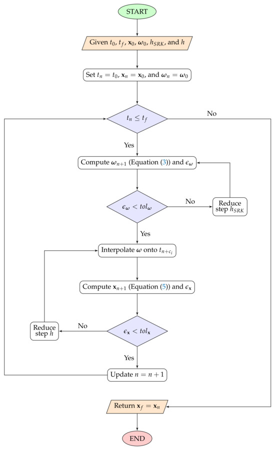
Figure 1.
Outline of the general deterministic-stochastic hybrid integrator with double adapting time step.
It is important to highlight that if the time step related to the ordinary RK scheme is adjusted, it is not necessary to integrate the stochastic state again, since a solution with the required tolerance already exists. Moreover, according to the selected adaptive time-stepping algorithm, the time step could be changed even when the step is accepted.
From the general outline in Figure 1, different hybrid integrators can be constructed by changing the method associated with each step, specifically:
- (1)
- (2)
- the SRK adaptive time-stepping algorithm,
- (3)
- the interpolation method, projecting the noise into the ordinary differential equation scheme,
- (4)
- the RK scheme from Equation (5), and
- (5)
- the RK time-stepping algorithm, associated to the deterministic step.
The choice of each of these items is bound to the characteristics of the differential equations system to be solved, the required accuracy, and the available computational resources.
3. Euler–Maruyama–Runge–Kutta Scheme
A relevant number of physical dynamical systems are characterized by
- (1)
- a simple stochastic dynamics, e.g., linear stochastic processes, and
- (2)
- desired stringent tolerances, that enable accurate retracing of the real-world system.
In these cases, high-order stochastic Runge–Kutta schemes and the stochastic step-varying algorithm may not be required. The stochastic dynamics are then integrated by exploiting a fixed-step Euler–Maruyama scheme, i.e.,
where is the increment in the Brownian path. The step-length size is selected a-priori. On the other hand, the dynamics in Equation (2a) should be integrated by exploiting high-order embedded pairs of ordinary Runge–Kutta schemes in order to guarantee accurate integration and an effective time-adaptive algorithm. In this work, the Dormand–Prince method [24] and the Verner’s most efficient Runge–Kutta 8(7) pair [25] are employed. This hybrid stochastic-deterministic method, built combining a fixed step Euler–Maruyama method with variable step ordinary Runge–Kutta schemes, is labeled the Euler–Maruyama–Runge–Kutta (EMRK) algorithm. EMRK will act as a prototype for this kind of hybrid integrator, with the aim of showing that they are able to deliver fast accurate solutions. The accuracy of the method can be easily improved by replacing the Euler–Maruyama scheme with any other stochastic Runge–Kutta method, such as SRA by [8].
However, within this kind of scheme, the deterministic time-stepping algorithms commonly used for solving ODEs cannot be exploited, since they will discard information about the future Brownian motion, which biases the sample statistics for the path. For this reason, a method preserving information about the future path when the step is rejected is built, adapting the Rejection Sampling with Memory (RSwM) algorithm [11] to the hybrid integrators. The main differences are that the step size is determined by the deterministic part of the RODE and the interpolation of the SDE solution onto the deterministic one must be taken into account. The Brownian bridge [26] will be exploited both to manage the variable step size and the noise interpolation. By the properties of the Brownian bridge, considering a general Brownian motion with , then
for .
Modified Rejection Sampling with Memory
Following the scheme outlined by the RSwM, the modified Rejection Sampling with Memory (mRSwM) algorithms use two stacks and , with the first containing future information and the latter the re-popped ones. Each element of the stacks is a tuple containing the integration time at which it is associated and the values of the Brownian motion in Equation (9), e.g., . It is important to note that the value of the noise is not saved in the stacks, but rather re-computed from scratch when needed. This is related to the fact that the Brownian bridge can be applied directly only to Brownian paths.
An overview on how the mRSwM works is given in Figure 2:
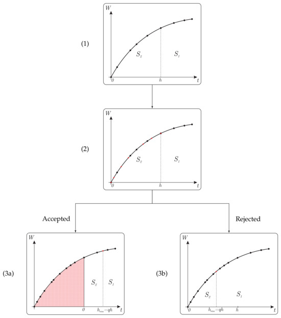
Figure 2.
Scheme for the adaptive time-step algorithm embedding mRSwM.
- (1)
- At a general time 0, the stacks and are not empty and contain future (i.e., after the time span h) and re-popped information (i.e., within the time span h), respectively. Note that even if could be empty, contains at least the values of the process at time 0;
- (2)
- The Brownian motion is interpolated in the time instants required by the ordinary RK algorithm (red dots in the figure) by exploiting the Brownian bridge and inserted into . Equation (2b) is integrated using Equation (9) and the information contained in . Later, Equation (2a) is solved by Equation (5).
- (3)
- In order to discern if the performed step should be accepted of rejected, the acceptable error is computed bywhere is the desired relative tolerance, and the step-size variation aswhere is the order of the ordinary Runge–Kutta scheme (e.g., 5 for the Dormand–Prince method).
- (3a)
- If , the step is accepted:is emptied. The information from within the new step length is later moved onto . Additionally, the element associated with the end of the new step should be added on top of by interpolating its last element with the first element of .
- (3b)
- If , the step is rejected:The information from within the new step length is moved onto , and the element associated with the end of the new step is added on top of by interpolating its last element with the first element of .
After that, this cycle is repeated until the final time is reached.
Moreover, special care should be paid when adding new elements to . Since the integration step for the stochastic part must be equal or lower than , if two elements in are separated in time by a greater interval, additional time steps should be added by exploiting the Brownian bridge. A pseudocode version of the mRSwM is given in Algorithm 1.
4. Results
In order to assess the performance of the hybrid Euler–Maruyama–Runge–Kutta method, tests on both correctness and efficiency are performed. The first kind of test evaluates the capability of EMRK to provide statistically correct solutions, while the latter compares the required computational effort against some known methods to solve RODEs. These tests are performed using two different dynamical systems to also evaluate the ability of EMRK to solve different kinds of systems.
4.1. Mass-Spring System
The first dynamic being tested is a simple mass-spring system with a forcing term described by a Gauss–Markov process, that can be written as
with m indicating the mass, k the elastic coefficient of the spring, and
Since the system is linear in both the deterministic and stochastic part, it can be conveniently written as
with . The system in Equation (15) has the solution
where is the white noise.
| Algorithm 1: Euler-Maruyama-Runge–Kutta scheme. |
 |
Even though Equation (16) cannot, in general, be evaluated, except in a statistical sense, due to the stochastic integral, it can be used to infer solution characteristics at a given time. Specifically, the mean
since , while the covariance is
where
given that .
Solutions of the EMRK are compared against the analytic solution and two different numerical schemes: (1) a 1.5-order stochastic scheme by Rossler [8] (labeled SRIW2), exploiting its adaptive-step implementation in Julia [27], and (2) a classic Dormand–Prince method (labeled ODE45). For the ODE45 case, the process noise is computed iteratively a-priori [19] in some prescribed points, meaning that the values
with , and . These values are later interpolated during the integration runtime at the time requested by the integrator, exploiting the same formula.
A Monte Carlo simulation of 1000 samples is employed to perform the tests, integrating the mass-spring system up to 4 s. Other simulation parameters are listed in Table 1.

Table 1.
Perturbed mass-spring dynamics parameters.
Results for the correctness analysis are shown in Figure 3. Visually comparing the histogram and the swarm charts, it can be inferred that all three algorithms are able to provide similar results. These results are confirmed by performing a one-sample Kolmogorov–Smirnov test [28]. The Kolmogorov–Smirnov test is a classical test used to compare a sample against a reference distribution, usually the normal Gaussian distribution. From Equation (15) it can be deduced that the system solution is still Gaussian. Thus, a simple and robust way to verify the correctness of the algorithm is to check if the solution has a distribution with the mean given by Equation (17) and variance in Equation (18). Figure 4 shows the Kolmogorov–Smirnov p-values of 20 samples made by 100 simulations. At a p-value of 0.05, it is expected to find 1/20 failed tests. Indeed, all the algorithms shows results around the expected number of failures. These results indicate that the mass-spring system at t = 4 s is still distributed as expected and the EMRK algorithm does not significantly alter the stochastic properties of the solution, neither do the other two algorithms, which can be used as exact solutions in the other test case where an analytic solution does not exist.
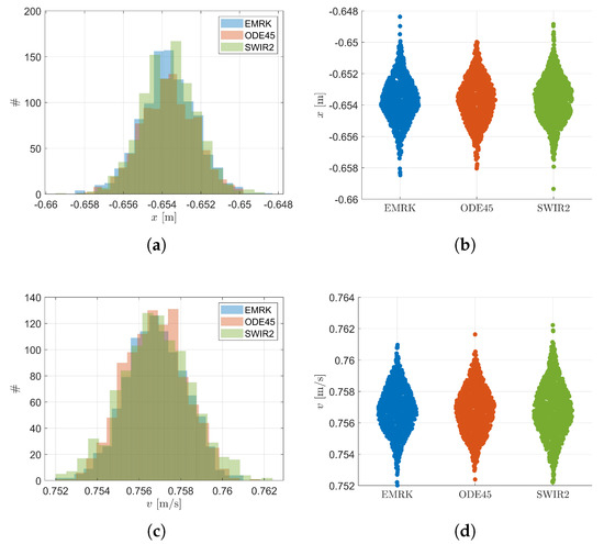
Figure 3.
Relevant statistics for the uncertain mass-spring system: (a) Histogram for the x-component of the state; (b) Swarm chart for the x-component of the state; (c) Histogram for the v-component of the state; (d) Swarm chart for the v-component of the state.
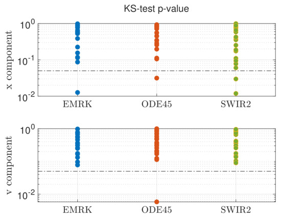
Figure 4.
p-values for the Kolmogorov–Smirnov Test at t = 4 s for the uncertain mass-spring system. The black dashed line marks p-value at 0.05.
Additionally, Figure 5 presents the Quantile–Quantile plots both for the position and the velocity, comparing the normalized state with respect to the standard Gaussian. The samples are distributed along the first-quadrant bisector, meaning that they follow a normal distribution as expected. These results confirm the correctness of the EMRK scheme for RODE integration.
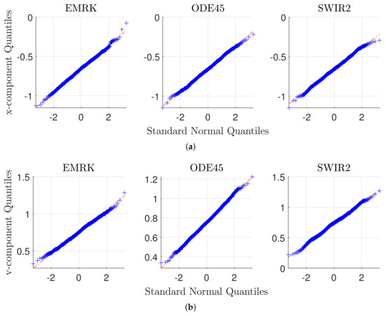
Figure 5.
Quantile–Quantile plots for the uncertain mass-spring system: (a) x-component of the state; (b) v-component of the state.
Figure 6 shows the statistics of the computational time for EMRK and ODE45 on an Intel i7@2.9 GHz with 16 GB RAM. This figure can be used to evaluate the efficiency of EMRK with respect to the other methods. EMRK is shown to be 10 times faster than ODE45, employing about 0.1 s to complete one integration. SWIR2 has not been shown since it is implemented in Julia and the comparison of its computational time with the other methods would not have been significant. However, for completeness’s sake, it was about 1.5 times slower than EMRK.
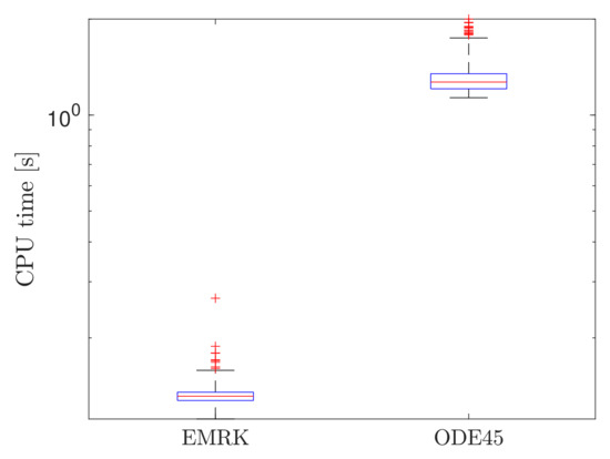
Figure 6.
Computational time statistics for the uncertain mass-spring system.
4.2. Restricted Two-Body Problem
The second dynamic being tested is a two-body problem, with uncertainty associated with unmodeled accelerations, considered as a Gauss–Markov process [29]
and
with being the identity matrix. The relevant parameters are listed in Table 2.
Table 2.
Perturbed two-body dynamics parameters.
Both accuracy and efficiency have been tested by running a Monte Carlo simulation with 1000 samples of a Hohmann transfer from the Earth to Mars, with an integration tolerance of . Differently from Section 4.1, a Verner’s most efficient Runge–Kutta 8(7) pair (labelled ODE78) is preferred to ODE45, since it is faster and more accurate for non-linear dynamical systems, requiring high-accuracy. The deterministic part of EMRK exploits the same integration scheme.
Figure 7 shows the statistics of the two-components of the position. As shown both in the histograms and the swarm charts, all the schemes are able to retrieve the same statistics for the transfer. Due to the non-linearity of the dynamics, an analytic solution does not exist. In this case, the SRIW2 solution will be used as reference, since SWIR2 has been proven to be effective in retrieving the correct statistics of a generic SDE [11]. A two-sample Kolmogorov–Smirnov test, comparing EMRK and ODE78 results to the SWIR2 reference result has been performed to confirm the results of Figure 7. In Figure 8, the p-value of the two-sample Kolmogorov–Smirnov test is shown for 20 samples. Each sample is made by 100 simulations. The failure rate considering a p-value of 0.05 is compatible with the theory. Thus, it is possible to conclude that EMRK is capable of accurately solving RODE problems under the assumptions made in Section 3, even in this more complex case. It also gives similar results to ODE78.
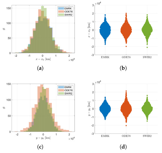
Figure 7.
Relevant statistics for the uncertain two-body problem: (a) Histogram for the x-component of the state; (b) Swarm chart for the x-component of the state; (c) Histogram for the y-component of the state; (d) Swarm chart for the y-component of the state.
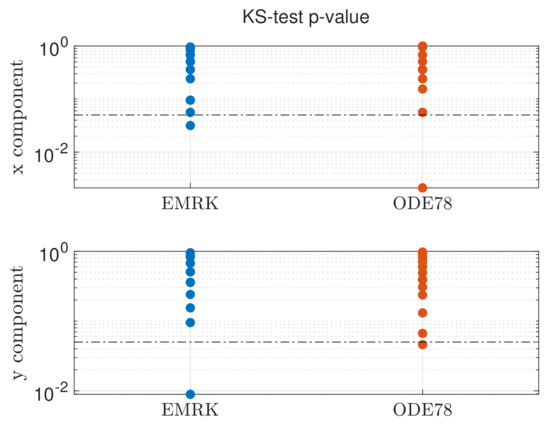
Figure 8.
p-values for the two-sample Kolmogorov–Smirnov test for the uncertain two-body problem system. The black dashed line marks p-value at 0.05.
Figure 9 shows the statistics of the computational time for EMRK and ODE78 in the uncertain two-body problem case. It can be inferred from the box plot that EMRK is able to integrate a single transfer in about 0.7 s, while ODE78 needs 30 times more. SWIR2, not shown in this plot due to its different implementation, has been two times slower than EMRK.
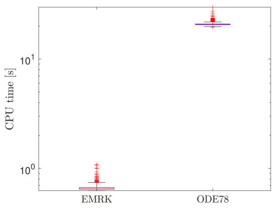
Figure 9.
Computational time statistics for the uncertain two-body problem.
5. Conclusions
In this work, a hybrid stochastic-deterministic integrator, labeled Euler–Maruyama–Runge–Kutta, has been presented. It was devised to solve random ordinary differential equations characterized by simple stochastic dynamics and requiring moderate-to-high tolerances, exploiting a modified RSwM algorithm to allow the step-size adaptation and increase the efficiency of the method.
EMRK is able to provide solutions that are statistically correct, while reducing by at least one order of magnitude the computational time with respect to state-of-the-art SDE solvers. Its implementation will be beneficial in running massive Monte Carlo simulations used in mission analysis and uncertainty quantification for space applications. However, it can also be exploited in different fields for various applications, such as risk assessments, end-of-life evaluation and dispersion analysis.
Funding
This work was partially carried out as part of CASTOR, a project that has received funding from the European Union’s Horizon Europe research and innovation program under the Marie Skłodowska-Curie grant agreement no. 101103826. This project has received funding from the European Research Council (ERC) under the European Union’s Horizon 2020 research and innovation program (grant agreement No. 864697).
Data Availability Statement
Dataset available on request from the author.
Conflicts of Interest
The author declares no conflicts of interest.
References
- Kloeden, P.E.; Platen, E. Numerical Solution of Stochastic Differential Equations; Springer: Berlin/Heidelberg, Germany, 1992. [Google Scholar] [CrossRef]
- Milstein, G.N.; Tretyakov, M.V. Stochastic Numerics for Mathematical Physics; Springer: Berlin/Heidelberg, Germany, 2004. [Google Scholar] [CrossRef]
- Burrage, K.; Burrage, P. General order conditions for stochastic Runge-Kutta methods for both commuting and non-commuting stochastic ordinary differential equation systems. Appl. Numer. Math. 1998, 28, 161–177. [Google Scholar] [CrossRef]
- Komori, Y. Weak second-order stochastic Runge–Kutta methods for non-commutative stochastic differential equations. J. Comput. Appl. Math. 2007, 206, 158–173. [Google Scholar] [CrossRef][Green Version]
- Komori, Y. Weak order stochastic Runge–Kutta methods for commutative stochastic differential equations. J. Comput. Appl. Math. 2007, 203, 57–79. [Google Scholar] [CrossRef]
- Rößler, A. Second order Runge–Kutta methods for Itô stochastic differential equations. SIAM J. Numer. Anal. 2009, 47, 1713–1738. [Google Scholar] [CrossRef]
- Newton, N.J. Asymptotically efficient Runge–Kutta methods for a class of Itô and Stratonovich equations. SIAM J. Appl. Math. 1991, 51, 542–567. [Google Scholar] [CrossRef]
- Rößler, A. Runge–Kutta methods for the strong approximation of solutions of stochastic differential equations. SIAM J. Numer. Anal. 2010, 48, 922–952. [Google Scholar] [CrossRef]
- Burrage, K.; Burrage, P.M. High strong order explicit Runge-Kutta methods for stochastic ordinary differential equations. Appl. Numer. Math. 1996, 22, 81–101. [Google Scholar] [CrossRef]
- Mukam, J.D.; Tambue, A. Strong convergence of a stochastic Rosenbrock-type scheme for the finite element discretization of semilinear SPDEs driven by multiplicative and additive noise. Stoch. Process. Their Appl. 2020, 130, 4968–5005. [Google Scholar] [CrossRef]
- Rackauckas, C.; Nie, Q. Adaptive methods for stochastic differential equations via natural embeddings and rejection sampling with memory. Discret. Contin. Dyn. Systems. Ser. B 2017, 22, 2731. [Google Scholar] [CrossRef] [PubMed]
- Tripura, T.; Gogoi, A.; Hazra, B. An Itô–Taylor weak 3.0 method for stochastic dynamics of nonlinear systems. Appl. Math. Model. 2020, 86, 115–141. [Google Scholar] [CrossRef]
- Wiktorsson, M. Joint characteristic function and simultaneous simulation of iterated Itô integrals for multiple independent Brownian motions. Ann. Appl. Probab. 2001, 11, 470–487. [Google Scholar] [CrossRef]
- Rybakov, K. Spectral representations of iterated stochastic integrals and their application for modeling nonlinear stochastic dynamics. Mathematics 2023, 11, 4047. [Google Scholar] [CrossRef]
- Cunha, A., Jr.; Sampaio, R. Uncertainty propagation in the dynamics of a nonlinear random bar. In Proceedings of the XV International Symposium on Dynamic Problems of Mechanics (Diname 2013), Buzios, Brazil, 17–22 February 2013. [Google Scholar]
- Bailey, N.; Hibberd, S.; Power, H.; Tretyakov, M. Effect of uncertainty in external forcing on a fluid lubricated bearing. In Proceedings of the International Conference on Rotor Dynamics; Springer: Cham, Switzerland, 2018; pp. 443–459. [Google Scholar]
- Luo, Y.Z.; Yang, Z. A review of uncertainty propagation in orbital mechanics. Prog. Aerosp. Sci. 2017, 89, 23–39. [Google Scholar] [CrossRef]
- Maybeck, P.S. Stochastic Models, Estimation, and Control; Academic Press: New York, NY, USA, 1982; Volume 3, pp. 180–185. [Google Scholar]
- Deserno, M. How to Generate Exponentially Correlated Gaussian Random Numbers; Department of Chemistry and Biochemistry, UCLA: Los Angeles, CA, USA, 2002. [Google Scholar]
- Han, X.; Kloeden, P.E. Random Ordinary Differential Equations; Springer: Singapore, 2017. [Google Scholar] [CrossRef]
- Grüne, L.; Kloeden, P.E. Higher order numerical schemes for affinely controlled nonlinear systems. Numer. Math. 2001, 89, 669–690. [Google Scholar] [CrossRef]
- Carbonell, F.; Jimenez, J.; Biscay, R.; De La Cruz, H. The local linearization method for numerical integration of random differential equations. BIT Numer. Math. 2005, 45, 1–14. [Google Scholar] [CrossRef]
- Jentzen, A.; Kloeden, P.E. Pathwise Taylor schemes for random ordinary differential equations. BIT Numer. Math. 2009, 49, 113–140. [Google Scholar] [CrossRef]
- Dormand, J.R.; Prince, P.J. A family of embedded Runge-Kutta formulae. J. Comput. Appl. Math. 1980, 6, 19–26. [Google Scholar] [CrossRef]
- Verner, J.H. Numerically optimal Runge-Kutta pairs with interpolants. Numer. Algorithms 2010, 53, 383–396. [Google Scholar] [CrossRef]
- Oksendal, B. Stochastic Differential Equations: An Introduction with Applications; Springer Science & Business Media: Heidelberg, Germany, 2013. [Google Scholar] [CrossRef]
- Rackauckas, C.; Nie, Q. DifferentialEquations.jl—Performant and Feature-Rich Ecosystem for Solving Differential Equations in Julia. J. Open Res. Softw. 2017, 5, 15. [Google Scholar] [CrossRef]
- Massey Jr, F.J. The Kolmogorov-Smirnov test for Goodness of Fit. J. Am. Stat. Assoc. 1951, 46, 68–78. [Google Scholar] [CrossRef]
- Schutz, B.; Tapley, B.; Born, G.H. Statistical Orbit Determination; Elsevier: Oxford, UK, 2004; Chapter 5. [Google Scholar] [CrossRef]
Disclaimer/Publisher’s Note: The statements, opinions and data contained in all publications are solely those of the individual author(s) and contributor(s) and not of MDPI and/or the editor(s). MDPI and/or the editor(s) disclaim responsibility for any injury to people or property resulting from any ideas, methods, instructions or products referred to in the content. |
© 2025 by the author. Licensee MDPI, Basel, Switzerland. This article is an open access article distributed under the terms and conditions of the Creative Commons Attribution (CC BY) license (https://creativecommons.org/licenses/by/4.0/).