Impact Analysis of Temperature Effects on the Performance of the Pick-Up Ion Analyzer

Abstract

In deep-space exploration, Pickup Ion Analyzers (PUIAs) operate under varying thermal environments in orbit, where thermally induced stress–deformation coupling may severely degrade their performance and long-term stability. To address temperature field analysis for in-orbit PUIAs, in this study, we propose a coupled simulation framework integrating external heat flux, parallel temperature field calculation, and thermoelastic deformation analysis, establishing a systematic link from thermal inputs to performance analysis. Based on external heat flux results, a parallel LU decomposition algorithm reduced the computational time from 11.8 h to 2.9 h for rapid temperature field solutions. At 38 astronomical units (AUs), the instrument’s temperature distribution ranged from −45 °C to 51.13 °C, with simulation errors compared to COMSOL simulations meeting engineering accuracy requirements. Maximum thermoelastic deformation induced by thermal gradients reached 0.110 mm. Performance degradation due to deformation in key metrics—including ion energy resolution, angular resolution, detection field-of-view, geometric factor, and mass resolution—was below 7.2%. This research improves the computational efficiency of the temperature field and systematically quantifies temperature effects on PUIA performance in deep-space environments, and the proposed methodology could provide technical support for optimizing on-orbit thermal management strategies.

1. Introduction

In deep-space exploration missions, fluctuations in spacecraft temperature caused by dynamic solar radiation lead to thermal deformation, thereby compromising the structural stability and detection capabilities of onboard instruments [1]. In Reference [2], Semena analyzed the Importance of Thermal Modes of Astrophysical Instruments in Solving Problems of Extra-Atmospheric Astronomy. Zhang et al. proposed a thermal design scheme for an Alpha Particle X-ray Spectrometer (APXS) in Reference [3], ensuring that APXS detectors and electronic devices operate within the allowable temperature range. However, these studies have been limited to the analysis of temperature fields and have not extended to investigating the impact of thermal variations on payload deformation and performance. The coupling between temperature and stress fields generates complex thermomechanical effects, significantly impacting ion detection and data analysis [4]. Consequently, it is imperative to comprehensively evaluate the performance of Pickup Ion Analyzers (PUIAs) in deep-space environments by integrating multiphysics coupling effects (e.g., thermal and stress fields) and systematically analyzing operational influences in orbit. Current simulation technologies for PUIAs often insufficiently consider thermo-structural coupling effects and lack analysis of their impact on performance [5,6]. Additionally, thermal field computation demands substantial resources and precise algorithms, with solving high-dimensional partial differential equations being a key technical challenge.

To accurately and efficiently simulate temperature effects on PUIA structures in deep-space environments and analyze performance considering deformation, while supporting thermal impact analysis under in-orbit conditions, research on temperature effects is needed. This paper addresses this by establishing a high-precision coupled simulation framework using finite element methods, incorporating external heat flux computation, parallel temperature field solving, and thermoelastic deformation analysis. Moreover, LU decomposition and multiprocess optimization techniques are employed for efficient temperature field computation.

The structure of this paper is as follows: In the next section, the concepts of the J2000 coordinate system and the orbital coordinate system and the construction method of the coordinate transformation matrix are reviewed; in Section 3, a high fidelity coupled simulation framework from thermal input to structural response is established; in Section 4, the external heat flow, temperature field, and thermal deformation are calculated, and the effect of thermoelastic deformation on the performance of the PUIA is analyzed; lastly, the conclusions of the paper are summarized and the outlook of future research is provided in Section 5.

2. Essential Preliminaries

Position calculation is the foundation for the analysis of external heat flux in spacecraft. The core objectives involve constructing the coordinate transformation matrix between the geocentric equatorial inertial coordinate system (J2000) and the orbital coordinate system, as well as acquiring the precise coordinates of the solar vector in the J2000 frame [7]. By establishing a unified spatiotemporal reference, the synergistic description of celestial positions and spacecraft attitude can be effectively achieved, thereby providing essential parametric support for the calculation of external heat flux angular coefficients. The following section delineates the spatiotemporal coordinate systems employed in the calculations presented in this study.

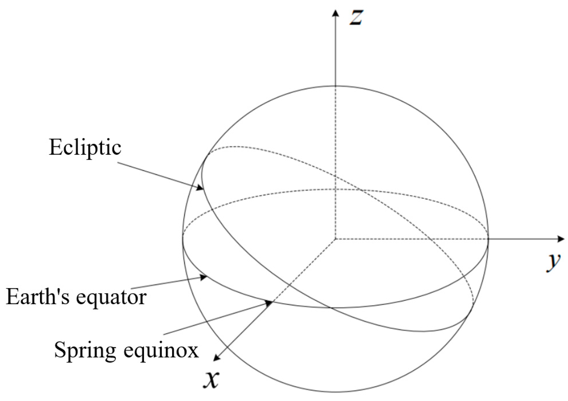
2.1. Geocentric Equatorial Inertial Coordinate System (J2000)

The geocentric equatorial inertial coordinate system (J2000) is defined with the Earth’s center of mass as its origin and the Earth’s equatorial plane as its reference plane and aligned with the mean equinox of J2000. Its temporal reference is fixed at 12:00 Terrestrial Time on 1 January 2000. This coordinate system, which does not rotate with Earth’s diurnal motion, is widely used in long-term celestial orbit prediction, deep-space navigation, and standardized computations of solar and planetary positions [8,9]. For solar vector calculations, the three-dimensional coordinates $(x,y,z)$ of the solar barycenter in the J2000 frame can be determined using astronomical constants (e.g., obliquity of the ecliptic, precession, and nutation) combined with stellar ephemeris algorithms. The z-axis aligns with Earth’s spin axis following the right-hand rule, while the y-axis forms a right-handed orthogonal system with the z- and x-axes, as illustrated in Figure 1 [10]. The coordinates are typically normalized in astronomical units (AUs), providing critical inputs for subsequent solar incidence angle analysis.

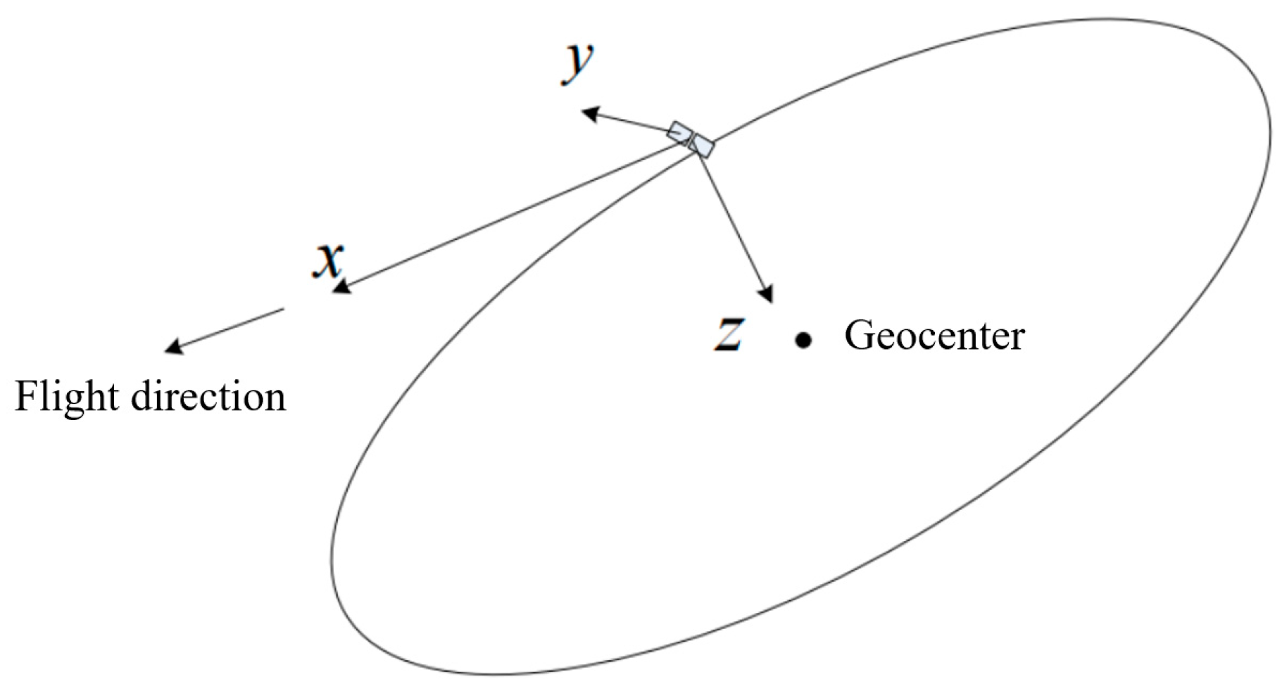
2.2. Orbital Coordinate System

The orbital coordinate system is defined with the payload center of mass of the spacecraft as its origin. Its basis vectors consist of the radial unit vector e_r (pointing toward the Earth’s center of mass), the transverse unit vector e_t (perpendicular to e_r within the orbital plane), and the normal unit vector e_n (determined by the right-hand rule as the orbital plane normal) [11]. In this system, the following conditions apply:

• The z-axis aligns with the geocentric direction.
• The x-axis lies within the satellite orbital plane, orthogonal to the z-axis, with its positive direction coinciding with the tangential direction of the spacecraft’s velocity vector.
• The y-axis completes a right-handed orthogonal triad with the x- and z-axes.

The axial definitions are intrinsically tied to the spacecraft’s spatial position and kinematic orientation. The spatial relationships are explicitly illustrated in Figure 2 [10].

2.3. Methodology for Constructing Coordinate Transformation Matrices

To establish the transformation relationship between the J2000 and orbital coordinate systems, a 4 × 4 homogeneous transformation matrix $T_{J2000}^{Orb}$ was generated through combined translation and rotation operations. The procedure comprises three principal stages:

• Origin Translation: Displace the J2000 origin to the spacecraft payload’s center of mass.
• Geocentric Axis Correction: Apply geocentric fixed rotation sequences to compensate for Earth’s rotational axis deviations.
• Orbital Plane Alignment: Orient the orbital basis vectors to coincide with the J2000 frame.

Mathematically, this transformation can be implemented via Rodrigues’ rotation formula or Euler angle decomposition. The final expression is formulated as follows:

$$T=\left[\begin{array}{cccc}{R}_Z(\psi )& R_Z(\psi )R_Y(\theta )& R_Z(\psi )R_Y(\theta )R_X(\varphi )& d^T\\ 0& 1& 0& t_z\\ 0& 0& 1& t_y\\ 0& 0& 0& 1\end{array}\right]$$

(1)

where:

• R denotes the composite rotation matrix.
• ψ, θ, and ϕ represent the orbital plane’s right ascension, inclination, and argument of latitude, respectively.
• d is the translation vector.
• t_x, t_y, and t_z constitute the time-dependent Earth rotation parameters.

This matrix comprehensively characterizes the spatiotemporal mapping relationship from the J2000 to the orbital coordinate system, ensuring rigorous coupling between celestial reference frames and spacecraft kinematics.

3. Proposed Method

Based on the space environment and satellite platform on which the PUIA operates, in this section, we analyze various environmental factors affecting the instrument’s performance, simulating environmental impact detection, and provide technical support for conducting simulation analysis of the payload under on-orbit working conditions.

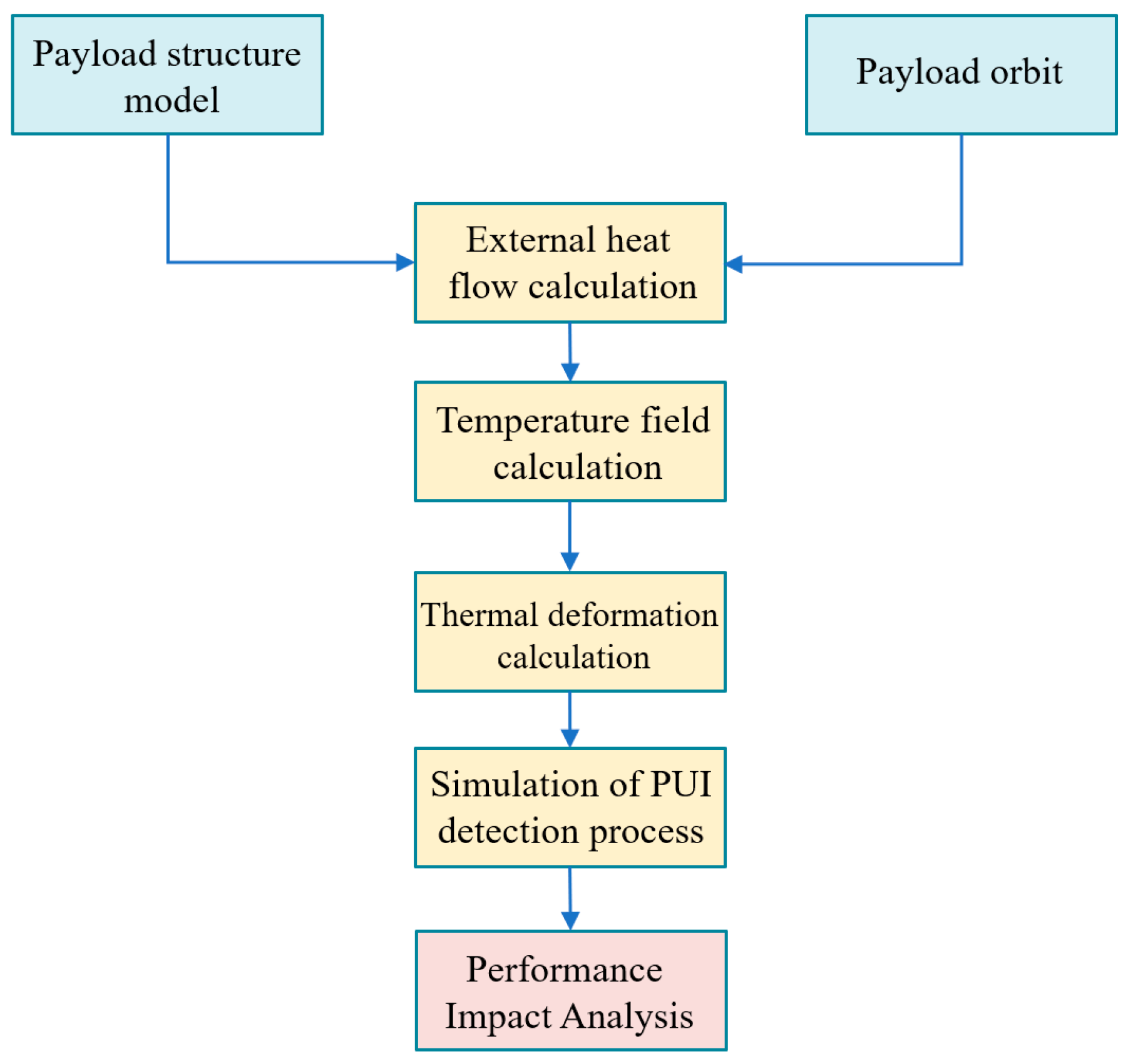
3.1. Temperature Effect Impact Simulation Method

Based on the analysis of deep-space environmental factors, the temperature effect was preliminarily identified as the most critical influence. The satellite was assembled under ground-level room-temperature conditions, while significant temperature variations occur during in-orbit operation, which affects both the satellite and payloads [12,13]. The impact of temperature fluctuations on PUIAs is currently unknown, as temperature can cause device deformation, which in turn affects performance.

To develop the temperature effect simulation framework and conduct numerical analyses, the following procedures need to be followed:

• External Heat Flux Calculation: Compute the external heat flux incident on the satellite surface based on its operational space environment.
• Thermal Distribution Simulation: Simulate temperature distributions and thermal deformations around the instrument using finite element methods, incorporating satellite structural and material properties.
• Performance Evaluation: Integrate deformation parameters into the PUIA detection simulation method to assess temperature-dependent influences on detection outcomes.

The flow chart for the impact analysis of temperature effects on the performance of the PUIA is illustrated in Figure 3.

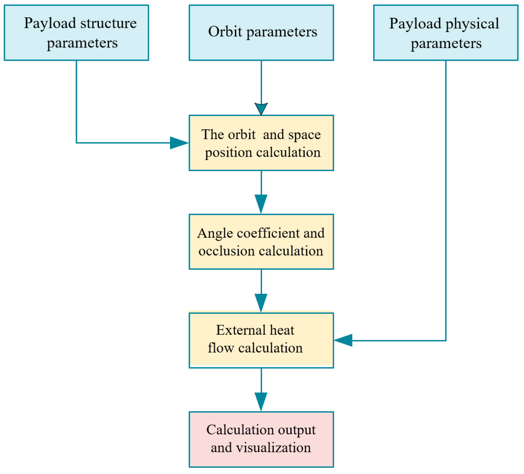
3.2. External Heat Flux Calculation Simulation Method

A thorough investigation of the external heat flux calculation simulation method revealed that the primary heat sources acting on the satellite during orbital operations consist of solar radiation, Earth-reflected solar radiation (albedo), and Earth infrared radiation [14]. In this study, the considered orbital range is approximately 38 AUs, where both Earth-reflected solar radiation and Earth infrared radiation become negligible. Consequently, solar radiation dominates as the principal external thermal source, and this work focuses exclusively on its computation. The key to calculating the solar radiation heat flow is to determine the spatial position of the orbit, judge the occlusion relationship, and determine the projected area of the object perpendicular to the sunlight. The solar radiation heat flux is calculated as the product of solar radiation intensity and the projected area [10]. The computational flow chart for payload external heat flux is illustrated in Figure 4.

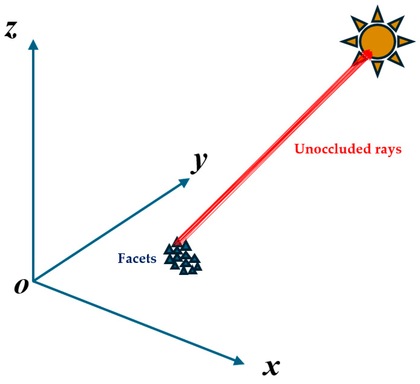
3.2.1. Occlusion Calculation

When calculating external heat flux, it is essential to calculate occultation between satellite structural components. Structural shadowing effects can be represented through inter-facet occlusion calculations [15]. Direct intersection testing between every emitted ray and all surface facets would incur computational overheads due to redundant evaluations. To optimize efficiency, a uniform grid partitioning scheme was implemented: the satellite structure model was subdivided into predefined grid cells, and the storage structure of facets was reorganized. Each facet is assigned to its corresponding grid cell based on spatial relationships. During occultation analysis, rays first undergo intersection tests with grid cells. Only rays intersecting a grid cell proceed to facet-level intersection checks within that cell, thereby eliminating unnecessary computations. Based on the finite element division, each triangular surface randomly emits N parallel rays in the direction of the Sun, as shown in Figure 5. Through the traversal algorithm, whether each ray intersects other surfaces along its propagation path is determined as follows:

• If a ray intersects with any facet other than the target facet, it is marked as occluded.
• If a ray exclusively interacts with the target facet without structural obstruction, it is counted as valid.

The effective projected area ratio of the target facet is determined by the proportion of unoccluded rays (n) to the total emitted rays (N).

The key advantage of this methodology lies in its probabilistic sampling approach, which circumvents the intricate boundary determination required in conventional geometric simulation. This proves particularly effective for analyzing occultation in satellites with complex configurations, such as multi-component assemblies or asymmetric structural geometries. Under deep-space conditions at 38 AUs, occultation effects from celestial bodies other than the satellite itself become negligible. Consequently, this analysis focuses exclusively on localized shadowing interactions between the satellite and its appendages.

The calculated results yield the angular coefficient through the following formula:

$$\eta ={\displaystyle \frac{n}{N}}$$

(2)

where n denotes the count of unoccluded rays and N represents the total number of emitted rays.

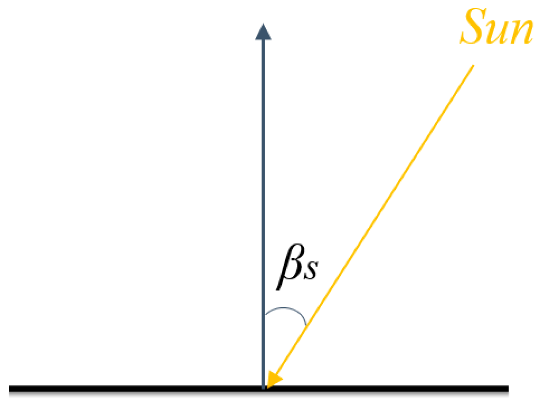
3.2.2. Methodology for External Heat Flux Calculation

For any given surface, calculating the received solar radiation heat flux involves determining the radiation flux corresponding to its projected area along the solar illumination direction. By treating sunlight as a collimated source with uniformly distributed radiation intensity (referred to as the solar constant S [10]), the solar vector in the satellite body coordinate system can be derived through orbital parameter analysis and coordinate transformation. Furthermore, the facet’s normal vector in the satellite body coordinate system is determined based on its vertex coordinates. Finally, the solar radiation angular coefficient ϕ is computed via dot and cross product operations:

$$\varphi =\cos {\beta }_s$$

(3)

where ${\beta }_s$ is the angle between the Sun’s rays and the plane’s normal vector, as shown in Figure 6.

The external solar radiation heat flow q of any facet is as follows:

$$q=S\cdot {\alpha }_s\cdot \varphi \cdot A$$

(4)

In the Formula (4), S represents the solar constant; ${\alpha }_s$ represents the solar radiation absorption rate of the plane element; ϕ represents the solar radiation angle coefficient, and A is the area of the triangular facet.

3.3. Parallel Temperature Field Computation Based on LU Decomposition

After acquiring the payload’s orbital parameters and external heat flux data, the temperature distribution of the PUIA can be calculated. Current methodologies for temperature field computation include techniques such as the thermal network method, the BP neural network method, and the finite element method (FEM). These approaches have been extensively applied across diverse fields [16,17,18,19,20,21,22,23]. Comparatively, the FEM discretizes the continuum into finite elements via variational principles, enabling accurate characterization of complex geometric boundaries, heterogeneous material properties, and multiphysics coupling effects [18]. Furthermore, the FEM has demonstrated mature applications in spacecraft thermal control design, and its inherent compatibility with structural mechanics analysis directly supports subsequent quantitative analysis of thermal-induced deformations on performance [19].

Therefore, in this study, we adopt the FEM as the core methodology for temperature field computation, optimizing computational efficiency, physical fidelity, and engineering feasibility. The workflow for temperature field computation of the PUIA is illustrated in Figure 7.

3.3.1. Target Equilibrium Equation

The PUIA structure model was first subjected to mesh generation, discretizing the geometry into 90,150 tetrahedral elements, with its exterior surface comprising 72,082 triangular facets, as shown in Figure 8. Although the external structure of the PUIA exhibits cylindrical symmetry, there are many components with non-axisymmetric features (such as internal channels, sensor parts, etc.) inside it, which require a mesh topology that can adapt to irregular boundaries. The tetrahedral unit performs well when partitioning complex geometric structures with arbitrary surface curvatures and internal interfaces, which is a classic method of partitioning. Therefore, the tetrahedral unit was selected for grid partitioning in this paper, which is consistent with the industry practice of hybrid geometry instruments in aerospace [24].

For thermal analysis targeting on-orbit satellites or payloads, the absence of convective heat transfer with the space environment due to the high vacuum of outer space allows for the elimination of convective terms in the energy balance equation. Additionally, since the orbit considered in this study is located at a distance of 38 AUs from the Sun, radiation from Earth and Earth-reflected solar radiation are neglected to simplify the calculations. The transient heat transfer process describes system heating/cooling dynamics where temperature distributions, heat flux rates, thermal boundary conditions, and internal energy exhibit time-dependent variations. Based on the energy conservation principle, the thermal equilibrium equation for each tetrahedral element is formulated as follows:

$$Q_{sun}+Q_{exchange}=Q_{self}+Q_{tempr}$$

(5)

(1)

Direct Solar Radiation (Q_sun) to the target unit P_i

The direct radiation Q_sun of the Sun to the unit P_i is the external heat flow calculated in Section 3.2. To calculate the direct solar radiation received by the payload, it is first necessary to determine whether the target is in the shaded area or the sunrise area. When the payload is directly irradiated by the Sun, the radiation intensity received by the target facet is closely related to the radiation angle coefficient of the Sun and the solar constant. In addition, the direct solar radiation received by each facet on the payload surface is also related to its area and absorption rate per unit area. Therefore, the geometric and radiation characteristics of the payload surface together determine the final radiation intensity.

$$Q_{sun}=\left\{\begin{array}{l}0\hspace{1em}\hspace{1em}\hspace{1em}\hspace{1em} ,shadow\\ S\cdot {\alpha }_s\cdot \varphi \cdot A, sunshine\end{array}\right.$$

(6)

In the formula, S represents the solar constant, and the size is 1353 W/m²; α_s represents the solar radiation absorption rate of the plane element; ϕ represents the solar radiation angle coefficient; and A is the area of the triangular facet.

(2)

The heat exchange (Q_exchange) between the target unit P_i and the adjacent unit P_j

The expression of the heat exchange Q_exchange between the target unit P_i and the adjacent unit P_j is established by considering the heat conduction exchange between the two units. Specifically, two units conduct heat flow through the contact surface, and the size of the heat flow is proportional to the temperature difference between the two nodes, and is related to the thermal conductivity of the two and the distance between the two units and the contact surface. Therefore, this heat exchange can be calculated using the following formula:

$$Q_{exchange}={\displaystyle \sum \frac{A_{ij}}{\frac{{\Delta }_i}{2K_i}+\frac{{\Delta }_j}{2K_j}}}\left(T_j-T_i\right)={\displaystyle \sum \frac{2K_i{K}_j{A}_{ij}}{{\Delta }_i{K}_j+{\Delta }_j{K}_i}}\left(T_j-T_i\right)$$

(7)

where A_ij represents the contact area between the unit P_i and the adjacent unit P_j; ${\Delta }_i$ and ${\Delta }_j$ represent the distance between the center of the unit P_i and the center of the unit P_j from the contact surface, respectively; K_i and K_j are the thermal conductivity of the unit P_i and the unit P_j, respectively; and T_i and T_j are the temperatures of the unit P_i and the unit P_j, respectively.

(3)

The heat radiated outward (Q_self) from the target unit P_i

The expression of heat Q_self radiated outward by the target unit P_i is based on the physical principle of heat radiation. It reflects the process by which the unit Pi radiates energy outward into space as a radiator. According to the Stefan–Boltzmann law, heat Q_self can be calculated using the following formula:

$$Q_{self}={\epsilon }_i\sigma A_i{T}_i^4$$

(8)

where ${\epsilon }_i$ represents the thermal emissivity of the unit P_i, that is, the ratio of the ability of the unit surface to radiate to the ability of the blackbody to radiate; σ represents the Stefan–Boltzmann constant, which has a value of about 5.67 × 10⁻⁸ W/m²K², which is a basic physical constant that describes the blackbody radiation power per unit area per unit temperature; A_i represents the surface area of the unit P_i; and T_i represents the temperature of the unit P_i.

(4)

Changes in the internal energy (Q_tempr) from the target unit P_i

The expression of Q_tempr for the change of internal energy in the target unit P_i is based on the principle of change of internal energy in thermodynamics. It describes the change of internal energy in the unit over time. Specifically, heat Q_tempr can be calculated using the following formula:

$$Q_{tempr}={(Gc)}_i{\displaystyle \frac{d{T}_i}{dt}}={\rho }_i{c}_i{v}_i{\displaystyle \frac{d{T}_i}{dt}}$$

(9)

where (Gc)_i represents the heat capacity of the unit P_i, representing the amount of heat required for each 1 degree change in the unit temperature; ρ_i is the density of the material of the unit P_i; c_i is the specific heat capacity of the unit P_i; v_i is the volume of the unit P_i; and dT_i/dt represents the rate of change in temperature over time.

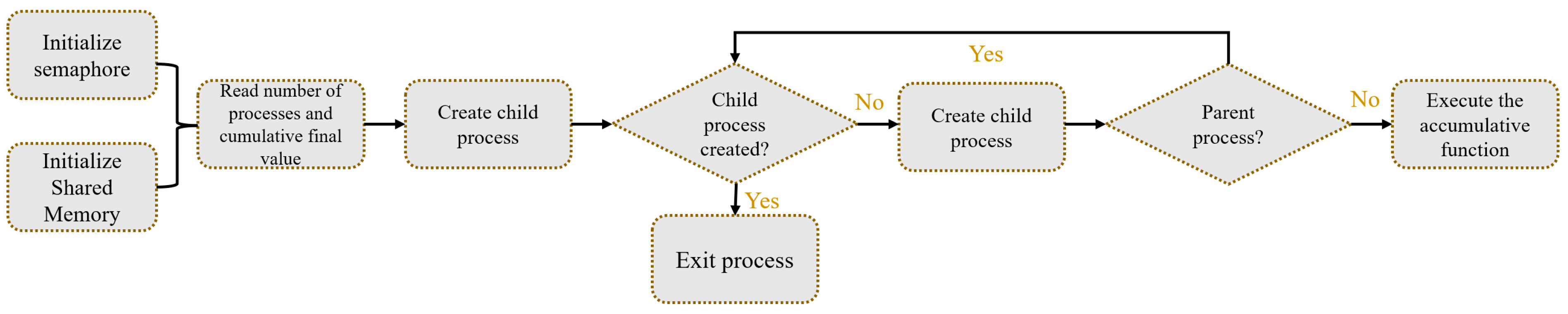
3.3.2. Solution of the Target Equilibrium Equation

The PUIA structure model was partitioned into 72,082 tetrahedral elements, denoted as N = 72,082. The FEM discretizes the continuum into finite elements via variational principles, enabling numerical solutions to the governing equations of heat transfer and thermoelastic deformation. The thermal equilibrium differential equations for each element contain time derivative terms and nonlinear terms involving the fourth power of temperature. To discretize these terms, the finite difference method was applied with the following transformations:

$${\displaystyle \frac{d{T}_i}{dt}}={\displaystyle \frac{T_i(t+\Delta t)-T_i}{\Delta t}}$$

(10)

$$T_i^4(t+\Delta t)=4T_i^3(t)(t+\Delta t)-3T_i^4(t)$$

(11)

Through this method, the specific discrete form of the differential equation of heat transfer of tetrahedral elements can be obtained:

$$\left[4{\varpi }_i{T}_i^3(t)+{\displaystyle \sum {\lambda }_{ij}}+{\displaystyle \frac{{(Gc)}_i}{\Delta t}}\right]T_i(t+\Delta t)-{\displaystyle \sum {\lambda }_{ij}}{T}_j(t+\Delta t)=3{\varpi }_i{T}_i^4(t)+{\displaystyle \frac{{(Gc)}_i}{\Delta t}}{T}_i(t)+Q_{sun}$$

(12)

where,

$${\varpi }_i={\epsilon }_i\sigma A_i, {\lambda }_{ij}={\displaystyle \frac{2K_i{K}_j{A}_{ij}}{{\Delta }_i{K}_j+{\Delta }_j{K}_i}}, \Delta t=0.05s$$

After linearizing the thermal equilibrium differential equations for all elements, a system of linear equations is obtained to solve the target temperature field. Let N denote the total number of discretized elements in the PUIA. For any element P_i, the following variable substitutions are implemented:

$$R_{ij}{T}_j(t+\Delta t)=y_i$$

(13)

The form could be rewritten into a matrix as follows:

$$RT(t+\Delta t)=Y$$

(14)

where

$$R_{ij}=\left[\begin{array}{cccc}{r}_{11}& r_{12}& \cdots & r_{1N}\\ r_{21}& r_{22}& \cdots & r_{2N}\\ ⋮& ⋮& \ddots & ⋮\\ r_{N1}& r_{N2}& \cdots & r_{NN}\end{array}\right], T(t+\Delta t)=\left[\begin{array}{c}{T}_1(t+\Delta t)\\ T_2(t+\Delta t)\\ ⋮\\ T_N(t+\Delta t)\end{array}\right], Y=\left[\begin{array}{c}{y}_1\\ y_2\\ ⋮\\ y_N\end{array}\right],$$

$$R_{ij}=\left\{\begin{array}{ll}{\displaystyle \sum {\lambda }_{ij}}& ,j\ne i\\ 4{\varpi }_i{T}_i^3(t)+{\displaystyle \sum {\lambda }_{ij}}+{\displaystyle \frac{{(Gc)}_i}{\Delta t}}& ,j=i\end{array}\right.$$

In summary, for each tetrahedral element, the heat balance equation is transformed into the following system of equations:

$$3{\varpi }_i{T}_i^4(t)+{\displaystyle \frac{{(Gc)}_i}{\Delta t}}{T}_i(t)+Q_{sun}=y_i$$

(15)

In order to improve the computational efficiency of solving the N × N linear equations (where N = 72,082), this paper considers the use of numerical calculation methods and multiprocessing libraries to solve the linear equations in parallel.

(i) Numerical Method Optimization

LU decomposition, a pivotal matrix factorization method in linear algebra [20], was adopted as the core numerical algorithm for solving the large-scale linear system derived from the thermal equilibrium equations. The rationale for selecting LU decomposition lies in its inherent structural advantages and computational efficiency improvements. Unlike direct Gaussian elimination, LU decomposition uniquely factorizes the coefficient matrix into a lower triangular matrix L and an upper triangular matrix U, decomposing the original system solution into two independent triangular system-solving processes. This approach not only eliminates potential numerical instability caused by repeated row exchange operations in Gaussian elimination but also optimizes computational resource allocation through pre-decomposition. Furthermore, within a parallel computing framework, LU decomposition enables distributed processing of matrix operations via multithreading techniques. For instance:

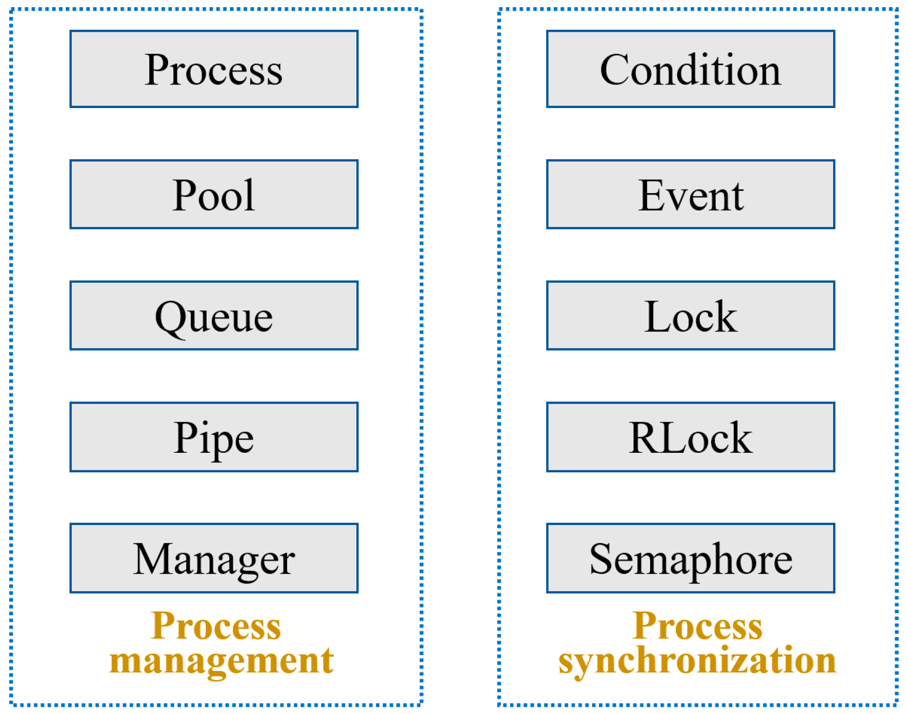
• Factorization Phase: Parallelization of independent row/column operations.
• Triangular System Solving: Concurrent execution of forward and backward substitution tasks across multicore architectures.

These strategies significantly reduce the solution time for large-scale linear systems. The detailed computational procedure is outlined below.

(a) LU decomposition: In matrix representation, the elimination process in Gaussian elimination involves performing a series of row elementary transformations on the augmented matrix A to convert the coefficient matrix into an upper triangular matrix U. This process is mathematically equivalent to left-multiplying the augmented matrix by a sequence of elementary matrices, simultaneously generating a lower triangular matrix L. Thus, the elimination procedure can be expressed as follows [21]:

$$A_{ij}=\left[\begin{array}{cccc}{r}_{11}& r_{12}& \cdots & r_{1N}\\ r_{21}& r_{22}& \cdots & r_{2N}\\ ⋮& ⋮& \ddots & ⋮\\ r_{N1}& r_{N2}& \cdots & r_{NN}\end{array}\begin{array}{c}{y}_1\\ y_2\\ ⋮\\ y_N\end{array}\right], L_{ij}=\left[\begin{array}{cc}\begin{array}{ccc}1& 0& 0\\ l_{21}& 1& 0\\ l_{31}& l_{32}& 1\end{array}& \begin{array}{ccc}\cdots & 0& 0\\ \cdots & 0& 0\\ \cdots & 0& 0\end{array}\\ \begin{array}{ccc}⋮& ⋮& ⋮\\ l_{n-1,1}& l_{n-1,2}& l_{n-1,3}\\ l_{n,1}& l_{n,2}& l_{n,3}\end{array}& \begin{array}{ccc}\ddots & ⋮& ⋮\\ \cdots & 1& 0\\ \cdots & l_{n,n-1}& 1\end{array}\end{array}\right],$$

$$U_{ij}=\left[\begin{array}{cc}\begin{array}{ccc}{u}_{11}& u_{12}& u_{13}\\ 0& u_{22}& u_{23}\\ 0& 0& u_{33}\end{array}& \begin{array}{ccc}\cdots & u_{1,n-1}& u_{1,n}\\ \cdots & u_{2,n-1}& u_{2,n}\\ \cdots & u_{3,n-1}& u_{3,n}\end{array}\\ \begin{array}{ccc}⋮& ⋮& ⋮\\ 0& 0& 0\\ 0& 0& 0\end{array}& \begin{array}{ccc}\ddots & ⋮& ⋮\\ \cdots & u_{n-1,n-1}& u_{n-1,n}\\ \cdots & 0& u_{nn}\end{array}\end{array}\right]$$

(b) Solving Le = b: Solve the equation composed of L and b using the forward substitution method to obtain the intermediate vector e.

$$Le=\left[\begin{array}{cc}\begin{array}{ccc}1& 0& 0\\ l_{21}& 1& 0\\ l_{31}& l_{32}& 1\end{array}& \begin{array}{ccc}\cdots & 0& 0\\ \cdots & 0& 0\\ \cdots & 0& 0\end{array}\\ \begin{array}{ccc}⋮& ⋮& ⋮\\ l_{n-1,1}& l_{n-1,2}& l_{n-1,3}\\ l_{n,1}& l_{n,2}& l_{n,3}\end{array}& \begin{array}{ccc}\ddots & ⋮& ⋮\\ \cdots & 1& 0\\ \cdots & l_{n,n-1}& 1\end{array}\end{array}\right]·\left[\begin{array}{c}\begin{array}{c}\begin{array}{c}{e}_1\\ e_2\end{array}\\ e_3\end{array}\\ ⋮\\ ⋮\\ e_N\end{array}\right]=\left[\begin{array}{c}\begin{array}{c}\begin{array}{c}{y}_1\\ y_2\end{array}\\ y_3\end{array}\\ ⋮\\ ⋮\\ y_N\end{array}\right]=Y$$

(c) Solve Ue = x: Solve the equation composed of U and e using the backward substitution method to obtain the final solution vector x.

$$Ue=\left[\begin{array}{cc}\begin{array}{ccc}{u}_{11}& u_{12}& u_{13}\\ 0& u_{22}& u_{23}\\ 0& 0& u_{33}\end{array}& \begin{array}{ccc}\cdots & u_{1,n-1}& u_{1,n}\\ \cdots & u_{2,n-1}& u_{2,n}\\ \cdots & u_{3,n-1}& u_{3,n}\end{array}\\ \begin{array}{ccc}⋮& ⋮& ⋮\\ 0& 0& 0\\ 0& 0& 0\end{array}& \begin{array}{ccc}\ddots & ⋮& ⋮\\ \cdots & u_{n-1,n-1}& u_{n-1,n}\\ \cdots & 0& u_{nn}\end{array}\end{array}\right]·\left[\begin{array}{c}\begin{array}{c}\begin{array}{c}{e}_1\\ e_2\end{array}\\ e_3\end{array}\\ ⋮\\ ⋮\\ e_N\end{array}\right]=\left[\begin{array}{c}\begin{array}{c}\begin{array}{c}{x}_1\\ x_2\end{array}\\ x_3\end{array}\\ ⋮\\ ⋮\\ x_N\end{array}\right]=x$$

The LU decomposition method reduces the computational amount of the equation system to a certain extent in the numerical method and improves the computational efficiency of the linear equation system. Since the LU decomposition is serial, this paper optimizes from the perspective of multiprocess, considering the steps in the Gaussian elimination process to speed up the calculation. The following describes the optimization process of multiprocess computing.

(ii) Multiprocess Computing Optimization

The computational efficiency for solving the N × N linear system (N = 72,082) is enhanced by using Python’s multiprocessing library through parallel computing. The core principle involves decomposing a computationally intensive task into smaller subtasks executed concurrently across multiple processor cores, thereby reducing overall computation time. Specifically, the acceleration strategy implemented in this study includes the following:

(a) Task Decomposition and Parallel Processing: The linear system is partitioned into N independent subtasks based on the row-wise and column-wise multiplication rules of matrices, which are distributed across available CPU cores.

(b) Latency Reduction: Concurrent execution of subtasks minimizes idle time between processes, optimizing computational resource utilization.

(c) Multicore CPU Exploitation: The multiprocessing library automatically allocates tasks to multiple processor cores, fully leveraging the capabilities of modern multicore architectures.

Python’s multiprocessing module provides cross-platform process control and inter-process communication functionalities. Its primary architectural components are illustrated in Figure 9.

The Process class is used to create, start, and terminate child processes; the Pool class is responsible for creating and managing process pools; the Queue, Pipe, and Manager classes provide inter-process communication and resource sharing functions; and the Condition, Event, etc., classes are used to implement process synchronization mechanisms. The flowchart of using the multiprocessing library to implement the multiprocess algorithm is shown in Figure 10.

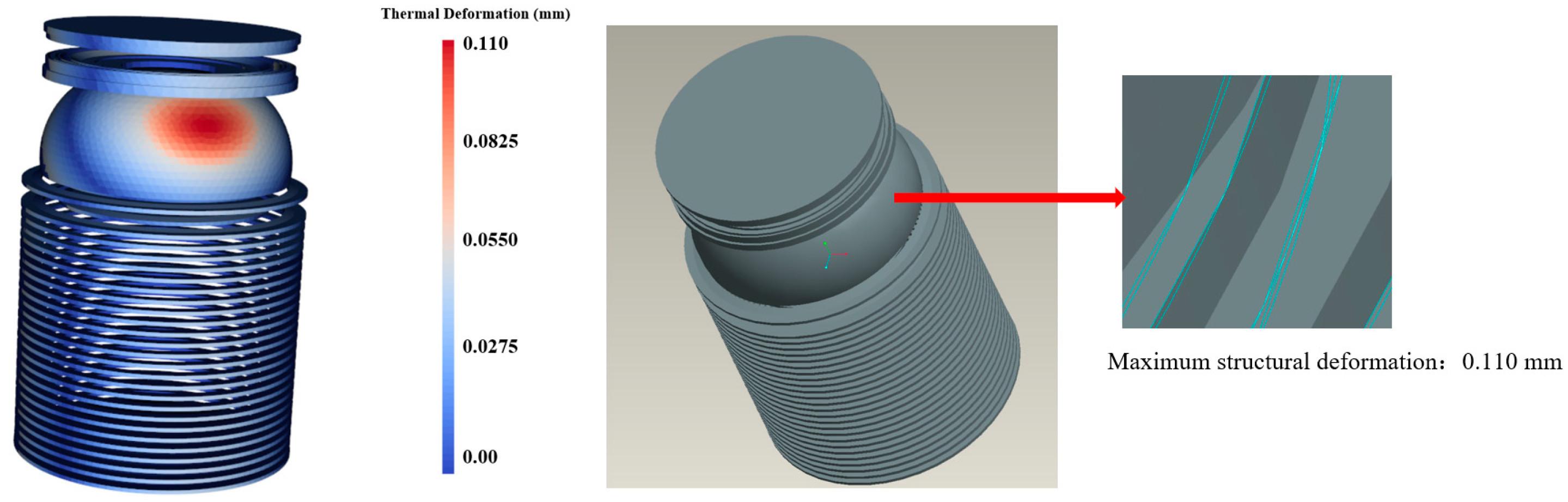
3.4. Calculation of Thermoelastic Deformation

Thermoelastic deformation refers to the mechanical response of materials caused by thermal expansion under temperature fields. Its quantitative analysis is critical for evaluating the performance degradation of the PUIA during on-orbit operations. Based on the computed temperature field and thermoelastic theory, in this section, we establish a thermal-structural coupling simulation method. The FEM is employed to solve deformation fields across instrument components under non-uniform temperature distributions, with further analysis of their compound effects on the PUIA’s performance. The flowchart of Thermoelastic Deformation Calculation is shown in Figure 11.

When subjected to temperature variations, the PUIA undergoes thermal deformation. To simulate the influence of temperature changes on its performance, we conducted numerical analyses of such deformations. For unconstrained structures, the relationship satisfies

$$\left\{\begin{array}{l}{\epsilon }_{xo}={\epsilon }_{yo}={\epsilon }_{zo}=\alpha t\\ {\gamma }_{xyo}={\gamma }_{yzo}={\gamma }_{zxo}=0\end{array}\right.$$

(16)

In this paper, only the case of isotropic materials is considered. $\epsilon$ denotes the normal strain, $\gamma$ is the shear strain, $\alpha$ is the coefficient of linear expansion, and t is the value of temperature change. Specifically, for isotropic objects, in the free state, changes in the temperature field usually cause only positive strain, not shear strain. However, in practical applications, objects are usually not in a state of complete free expansion or contraction, which results in the creation of external constraints that can induce thermal deformation [23]. According to the generalized Huke’s law:

$$\left\{\begin{array}{l}{\epsilon }_x={\displaystyle \frac{\partial u}{\partial x}}={\displaystyle \frac{1}{E}}\left[{\sigma }_x-\mu ({\sigma }_y+{\sigma }_z)\right]+\alpha t\\ {\epsilon }_y={\displaystyle \frac{\partial v}{\partial y}}={\displaystyle \frac{1}{E}}\left[{\sigma }_y-\mu ({\sigma }_z+{\sigma }_x)\right]+\alpha t\\ {\epsilon }_z={\displaystyle \frac{\partial w}{\partial z}}={\displaystyle \frac{1}{E}}\left[{\sigma }_z-\mu ({\sigma }_x+{\sigma }_y)\right]+\alpha t\\ {\gamma }_{xy}={\displaystyle \frac{{\xi }_{xy}}{G}}\\ {\gamma }_{yz}={\displaystyle \frac{{\xi }_{yz}}{G}}\\ {\gamma }_{zx}={\displaystyle \frac{{\xi }_{zx}}{G}}\end{array}\right.$$

(17)

where $\epsilon$ represents the normal strain, σ represents the normal stress, $\gamma$ represents the shear strain, $\xi$ represents the shear stress, and u, v, and w are the displacement components along the three coordinate axes. E, μ, and G represent the tensile (or compressive) modulus of elasticity, Poisson’s ratio, and shear modulus of the material, respectively, which are all proportional factors. For isotropic materials, the correlation can be expressed as follows:

$$G={\displaystyle \frac{E}{2(1+\mu )}}$$

(18)

Create the equilibrium differential equation as follows:

$$\left\{\begin{array}{l}(\lambda +G){\displaystyle \frac{\partial \psi }{\partial x}}+G{\nabla }^{2}u-\varsigma {\displaystyle \frac{\partial t}{\partial x}}+X=0\\ (\lambda +G){\displaystyle \frac{\partial \psi }{\partial y}}+G{\nabla }^{2}v-\varsigma {\displaystyle \frac{\partial t}{\partial y}}+Y=0\\ (\lambda +G){\displaystyle \frac{\partial \psi }{\partial z}}+G{\nabla }^{2}w-\varsigma {\displaystyle \frac{\partial t}{\partial z}}+Z=0\end{array}\right.$$

(19)

where X, Y, and Z represent the components of the volumetric force per unit volume, $\lambda$ represents the Lame constant, $\psi$ represents the volumetric strain, and $\varsigma$ represents the thermal stress coefficient, and the following relationship is satisfied:

$$\lambda ={\displaystyle \frac{E\mu }{(1+\mu )(1-2\mu )}}$$

(20)

$$\psi ={\epsilon }_x+{\epsilon }_y+{\epsilon }_z$$

(21)

$$\varsigma ={\displaystyle \frac{\alpha E}{1-2\mu }}$$

(22)

Therefore, the following equations are established:

$$\left\{\begin{array}{l}{\epsilon }_x={\displaystyle \frac{\partial u}{\partial x}},{\epsilon }_y={\displaystyle \frac{\partial v}{\partial y}},{\epsilon }_z={\displaystyle \frac{\partial w}{\partial z}}\\ {\gamma }_{xy}={\displaystyle \frac{\partial v}{\partial x}}+{\displaystyle \frac{\partial u}{\partial y}},{\gamma }_{yz}={\displaystyle \frac{\partial w}{\partial y}}+{\displaystyle \frac{\partial v}{\partial z}},{\gamma }_{zx}={\displaystyle \frac{\partial u}{\partial z}}+{\displaystyle \frac{\partial w}{\partial x}}\end{array}\right.$$

(23)

$$\left\{\begin{array}{l}{\displaystyle \frac{{\partial }^2{\epsilon }_x}{\partial y^2}}+{\displaystyle \frac{{\partial }^2{\epsilon }_y}{\partial x^2}}={\displaystyle \frac{{\partial }^2{\gamma }_{xy}}{\partial x\partial y}}\\ {\displaystyle \frac{{\partial }^2{\epsilon }_y}{\partial z^2}}+{\displaystyle \frac{{\partial }^2{\epsilon }_z}{\partial y^2}}={\displaystyle \frac{{\partial }^2{\gamma }_{yz}}{\partial y\partial z}}\\ {\displaystyle \frac{{\partial }^2{\epsilon }_z}{\partial x^2}}+{\displaystyle \frac{{\partial }^2{\epsilon }_x}{\partial z^2}}={\displaystyle \frac{{\partial }^2{\gamma }_{zx}}{\partial z\partial x}}\\ {\displaystyle \frac{\partial }{\partial x}}\left({\displaystyle \frac{\partial {\gamma }_{zx}}{\partial y}}+{\displaystyle \frac{\partial {\gamma }_{xy}}{\partial z}}-{\displaystyle \frac{\partial {\gamma }_{yz}}{\partial x}}\right)=2{\displaystyle \frac{{\partial }^2{\epsilon }_x}{\partial y\partial z}}\\ {\displaystyle \frac{\partial }{\partial y}}\left({\displaystyle \frac{\partial {\gamma }_{xy}}{\partial z}}+{\displaystyle \frac{\partial {\gamma }_{yz}}{\partial x}}-{\displaystyle \frac{\partial {\gamma }_{zx}}{\partial y}}\right)=2{\displaystyle \frac{{\partial }^2{\epsilon }_y}{\partial z\partial x}}\end{array}\right.$$

(24)

Using the aforementioned equations and corresponding boundary conditions, the displacements and deformations of the structure can be solved. Based on this methodology, a quantitative relationship between the temperature field and thermoelastic deformation is established, thereby enabling the determination of deformation magnitudes according to the spatial distribution of the temperature field.

4. Experiment and Results

During the construction of the temperature effect influence method, a series of fundamental assumptions must be introduced to simplify the mathematical description of complex physical processes while ensuring method feasibility and practicality.

Assumption 1.

The material properties of the PUIA (including thermal conductivity, specific heat capacity, and coefficient of thermal expansion) are assumed to remain constant within the operational temperature range, neglecting the effects of material phase transitions or nonlinear thermodynamic behaviors.

Assumption 2.

The thermal conduction process within the PUIA is treated as quasi-steady-state, where the temperature field’s temporal variation rate is significantly lower than the thermal conduction response time. This permits the application of steady-state heat conduction equations for approximate solutions. Regarding the structural deformation of PUIA, the aluminum alloy material used in the PUIA structure has a fatigue limit of 223 MPa under the condition of multi-cycle stress [25]. In addition, studies have shown that [26] the creep–fatigue interaction of aluminum alloy in the deep-space thermal environment below 100 °C can be ignored, thereby precluding nonlinear structural responses or failure mechanisms.

Assumption 3.

Temperature-induced structural deformations are postulated to primarily affect the geometric parameters of the PUIA (e.g., aperture dimensions, inter-electrode spacing), while their impacts on electromagnetic field distribution and ion trajectory characteristics can be approximated through linearization techniques.

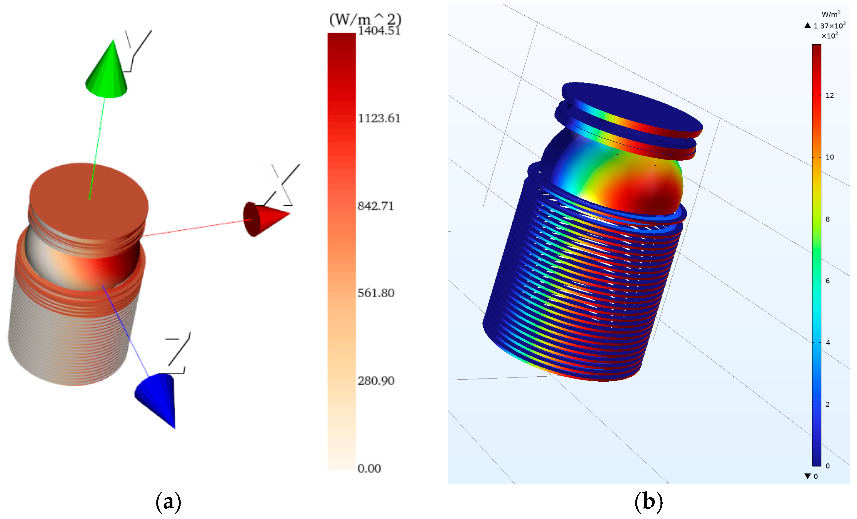
4.1. External Heat Flux Calculation Results

In this section, according to the external heat flow calculation method established in Section 3.2, we calculated the external heat flow based on the relevant parameters in

Table 1. External heat flow calculation parameter setting.

Parameter Name	Symbol	Value	Unit/Note
Solar constant *	$S$	1353	W/m2
Solar radiation absorption rate *	${\alpha }_s$	0.7	Dimensionless
Number of grid cells	$N_W$	90,150	Tetrahedral Unit
Number of surface pieces	$N_B$	72,082	Triangle Dlice
Track radius	R	38	AU

* Parameter source: References [10,14].

.

Based on the parameters listed in Table 1, the PUIA was divided into tetrahedrons using the FEM, and the partition view is shown in Figure 12.

Based on the operational orbit of the PUIA and the data structure of tetrahedral partitioning, the external surfaces were extracted through topological relationships between triangular vertices and their constituent facets. The calculated shadowing effects were then integrated to determine the external heat flux distribution across each facet, as shown in the left-hand panel of Figure 13. To validate the computational results, COMSOL Multiphysics 6.2^® [22] simulations were conducted, with the numerical verification results presented in the right-hand panel of Figure 13.

The computational results showed that the maximum heat flux density on the sunlit side of the instrument reaches 1404.51 W/m², while in shadowed regions, it approaches zero. To validate the method’s accuracy, the calculated results were compared with COMSOL Multiphysics 6.2^® simulations. The percentage error distribution between the two methods is visualized in Figure 14.

As shown in the figure above, the mean percentage error between the computational results of the proposed external heat flux method and COMSOL Multiphysics 6.2^® simulations is 3.22%. To further elucidate the error distribution characteristics, the error percentage values were subjected to Gaussian fit analysis, with their distribution presented in Figure 15.

As shown in Figure 15, the percentage relative error in the external heat flux calculations follows a Gaussian distribution with a mean (μ) of 3.22% and a standard deviation (σ) of 1.55%. According to the three-sigma rule of normal distribution, 99.74% of data points are expected to lie within the interval (μ − 3σ, μ + 3σ). In this study, the upper bound at μ + 3σ corresponds to 7.87%, indicating a 99.74% probability that the discrepancy between the proposed method and COMSOL Multiphysics 6.2^® simulations remains below this threshold. The central tendency of the error (3.22 ± 1.55%) confirms the close agreement between the computational methodology and numerical simulations.

Validated by these results, the external heat flux calculations will serve as key boundary conditions in the subsequent sections for conducting quantitative investigations of the temperature field in the PUIA.

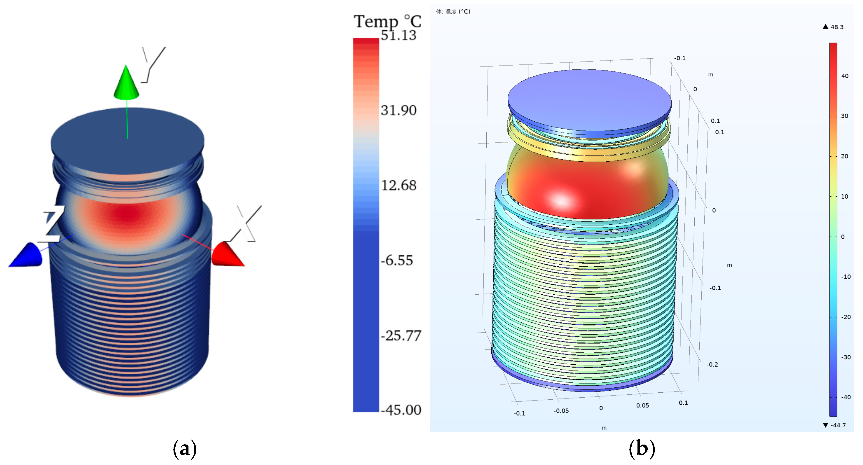
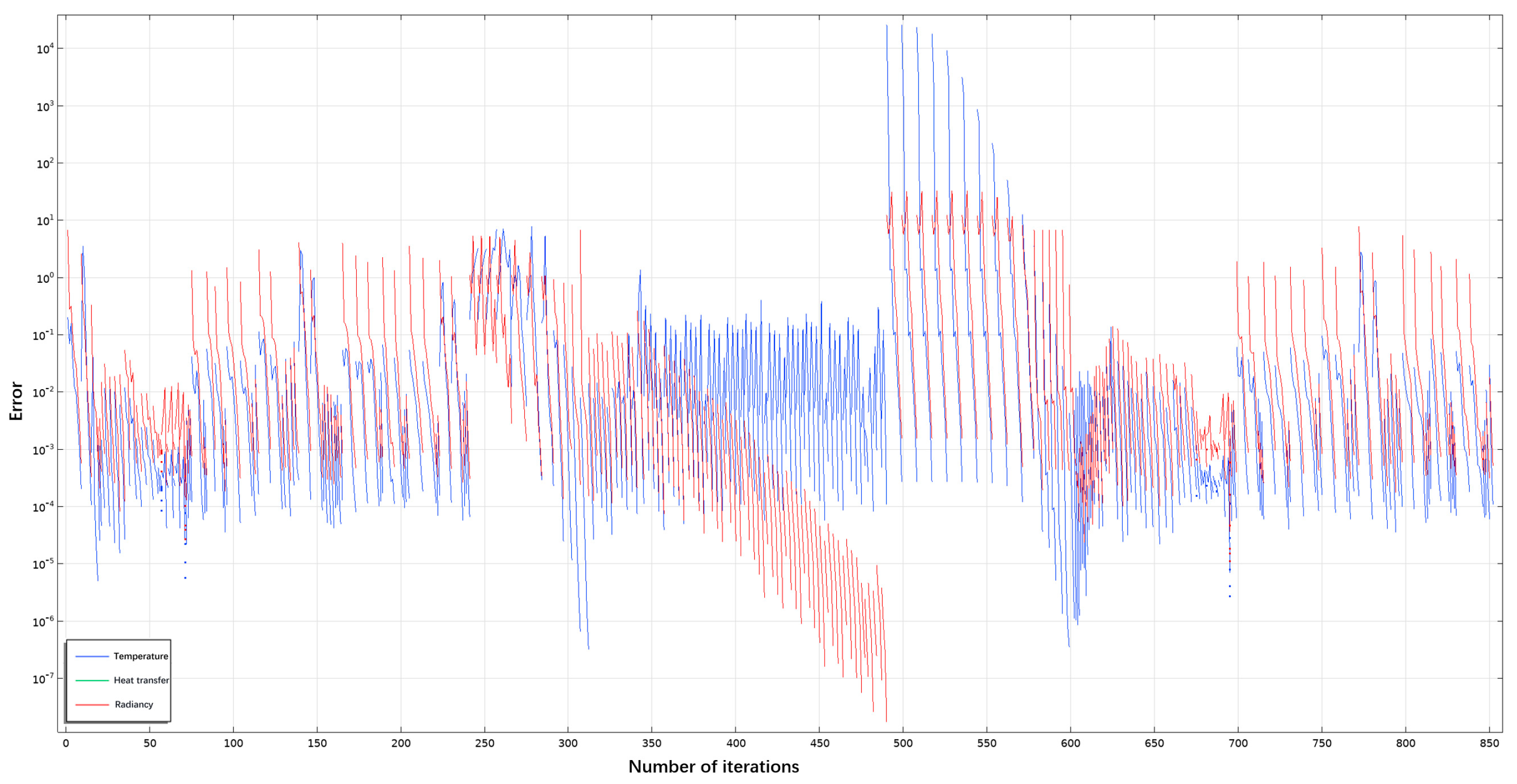
4.2. Temperature Field Calculation Results

In this subsection, the temperature field of the PUIA is calculated based on the established temperature field computational method and the relevant parameters listed in

Table 2. Temperature field calculation parameter setting.

Parameter Name	Symbol	Value	Unit/Note
Constant pressure heat capacity *	$C_p$	900	J/(kg·K)
Density	$\rho$	3900	kg/m3
Thermal conductivity *	$k$	27	W/(m·K)
Coefficient of thermal expansion	$\alpha$	8 × 10−6	1/K
Young’s modulus	E	300	GPa
Boltzmann constant *	$\sigma$	5.67 × 10−8	W/(m2·K2)
Poisson’s ratio	$\lambda$	0.222	Dimensionless

* Parameter source: References [11,13].

.

The PUIA, constructed from aluminum alloy, was numerically analyzed using the FEM. A transient heat conduction method coupled with radiation boundary conditions was implemented, with computational acceleration achieved through LU decomposition and multiprocess parallel optimization techniques. The resultant temperature field distribution is presented in Figure 16, and the simulation time, which corresponds to the 3D temperature field in Figure 16, is 10,440 s.

The convergence graph of the PUIA temperature field numerical solution provided by COMSOL is shown in Figure 17. It can be seen from the figure that the blue line represents the temperature value. As the number of iterations increases, the error value converges to 6 × 10⁻⁵~3 × 10⁻².

The parallel temperature field computation based on LU decomposition reveals significant spatial temperature variations across the PUIA surface under steady-state conditions due to solar occultation, with temperatures ranging from −45 °C to 51.13 °C. To validate the method’s accuracy, the computational results were compared against COMSOL Multiphysics 6.2^® simulations. The percentage error distribution between the two methods is visualized in Figure 18.

A comparative analysis with COMSOL Multiphysics 6.2^® simulations revealed that the mean percentage error between the computational results of the proposed external heat flux method and numerical benchmarks is 4.39%. For enhanced clarity in error distribution analysis, the temperature field percentage error values were subjected to Gaussian fit analysis, with the resultant distribution presented in Figure 19.

As shown in Figure 19, the percentage relative error in temperature field calculations follows a Gaussian distribution with a mean (μ) of 4.39% and a standard deviation (σ) of 1.66%. According to the three-sigma rule of normal distribution, 99.74% of data points are expected to reside within the interval (μ − 3σ, μ + 3σ). In this study, the upper bound at μ + 3σ corresponds to 9.38%, indicating a 99.74% probability that discrepancies between the proposed method and COMSOL Multiphysics 6.2^® simulations remain below this threshold. The observed errors primarily arise from insufficient local mesh refinement in finite element partitioning and simplified assumptions in the approximate calculation of radiation angular coefficients. Nevertheless, the overall agreement (central tendency: 4.39 ± 1.66%) confirms strong consistency between the computational and simulated results, satisfying engineering analysis requirements.

To validate the stability of the numerical temperature solution, the following numerical stability analyses were conducted: 1. Time steps of 0.01 s, 0.03 s, 0.05 s, and 0.1 s were selected to compute the temperature field. 2. Surface piece quantities of 12,011, 43,675, 72,082, and 106,800 were selected to compute the temperature field. A comparative diagram of average errors between the computed temperature fields (in both cases) and the COMSOL simulation results is provided below.

As demonstrated in Figure 20, the computational error of the temperature field exhibits minor oscillations with varying time steps, yet these fluctuations remain below 1.5%. This confirms the numerical stability of the temperature solution. The number of surface pieces increased from 12,011 to 106,800, and the average error was significantly reduced from 8.06% to 3.02%, verifying the convergence of mesh refinement.

Furthermore, the LU decomposition and multiprocess parallel optimization reduced the computational time from 11.8 h (single-threaded) to 2.9 h (75.4% reduction), while the residual convergence iterations decreased from 426 to 84 (80.28% reduction). The comparative performance of algorithmic optimization is illustrated in Figure 21, validating the enhanced efficiency and numerical stability of the proposed methodology.

According to the experimental results, the following conclusions can be drawn:

• Sunlit surfaces exhibit thermal energy accumulation due to high absorptivity and low emissivity, resulting in localized temperatures 96.13 °C higher than shadowed surfaces.
• Shadowed surfaces approach the space environment baseline temperature under deep-space background radiation.

These results provide critical inputs for subsequent thermal–structural coupling analysis. The quantitative correlations between temperature gradients and thermoelastic deformations will be detailed in the following subsection.

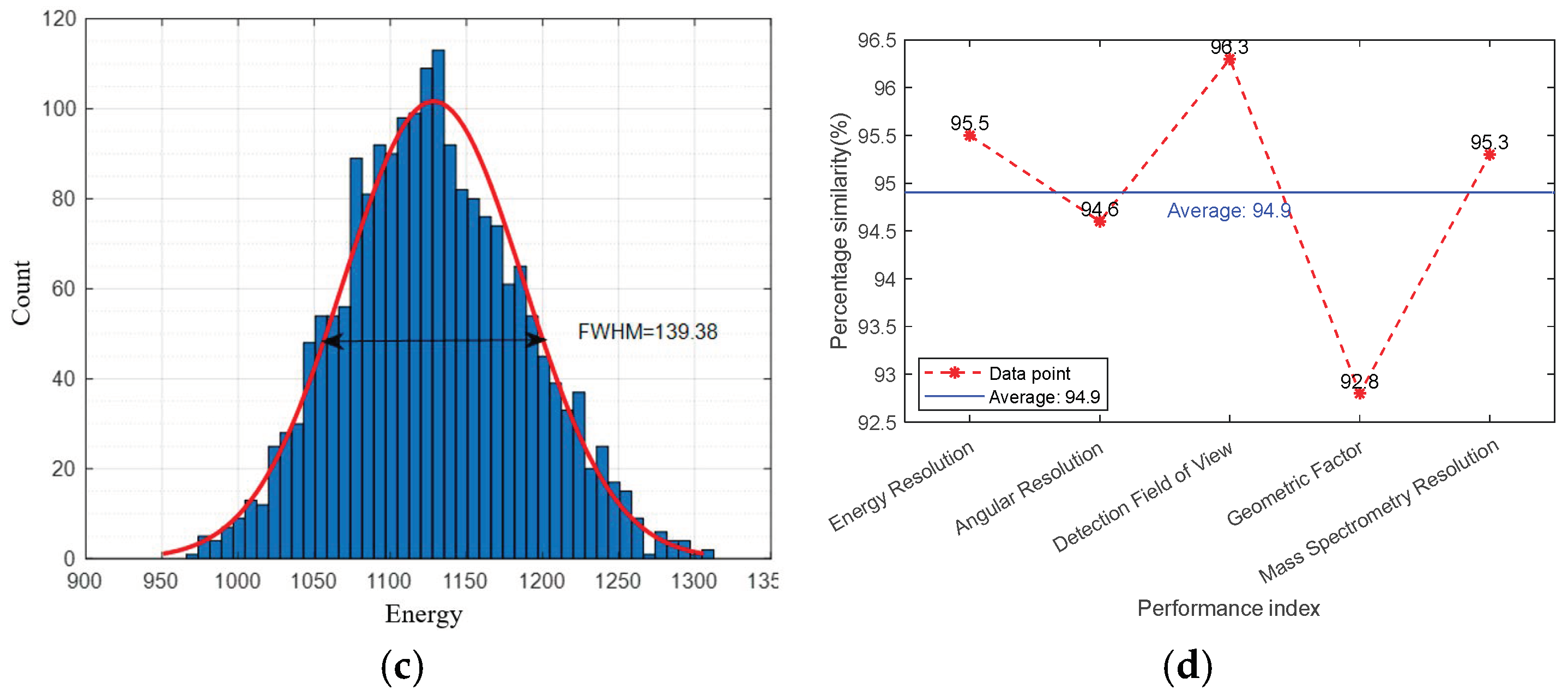
4.3. Impact of Thermoelastic Deformation on the PUIA’s Performance

Based on the finite element thermal-structural coupled simulation results, the maximum thermoelastic deformation of the PUIA induced by temperature gradients during on-orbit operations reaches 0.110 mm. The structural diagram of the PUIA after thermal deformation is shown in Figure 22. The simulation time, which corresponds to the 3D deformation field in Figure 22, is 289 s.

The spatial distribution of thermoelastic deformations exhibits a significant correlation with the temperature field. Sunlit surface facets experience maximum radial displacement of 0.110 mm due to thermal expansion under elevated temperatures, while shadowed support structures demonstrate maximum axial contraction of 0.088 mm induced by cryogenic shrinkage effects. This non-uniform deformation induces systematic deviations in critical geometric parameters of the ion electric field system. To analyze the impact of temperature effects on the PUIA’s performance in-orbit, this study applies the methodology outlined in [6] to simulate the post-deformation structure of the PUIA. The simulation results and performance impact analysis are schematically illustrated in Figure 23.

Simulation results of post-thermal deformation performance metrics revealed that temperature variations induce localized inter-electrode spacing increases of 0.12–0.37%. However, the energy resolution remains at 95.5% of its pre-deformation value (a reduction of 4.5%). Axial contraction on shadowed surfaces causes ion incidence channel misalignment, yet the angular resolution retains 94.6% of its original performance (a reduction of 5.4%). The field-of-view similarity reaches 96.3% (a reduction of 3.7%). The geometric factor decreases to 92.8% of its initial value, primarily due to cumulative geometric deviations reducing the effective ion detection area. The mass resolution retains 95.3% of its pre-deformation performance, indicating moderate thermal deformation effects on ion time-of-flight characteristics.

In conclusion, these experimental results demonstrate minor impacts of temperature effects on the performance of the PUIA. The instrument exhibits high stability (performance retention >90% across all critical metrics) in deep-space thermal environments, validating its robust thermo-mechanical design and operational reliability under extreme thermal gradients.

5. Conclusions

In this study, we establish a simulation framework to systematically investigate the impact of varying thermal environments on the performance of a PUIA. Based on the assumptions proposed in Section 4, the relevant experiments were carried out, and the following conclusions were obtained:

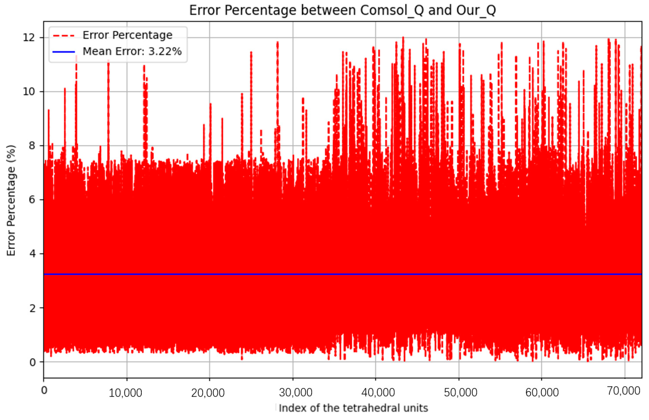
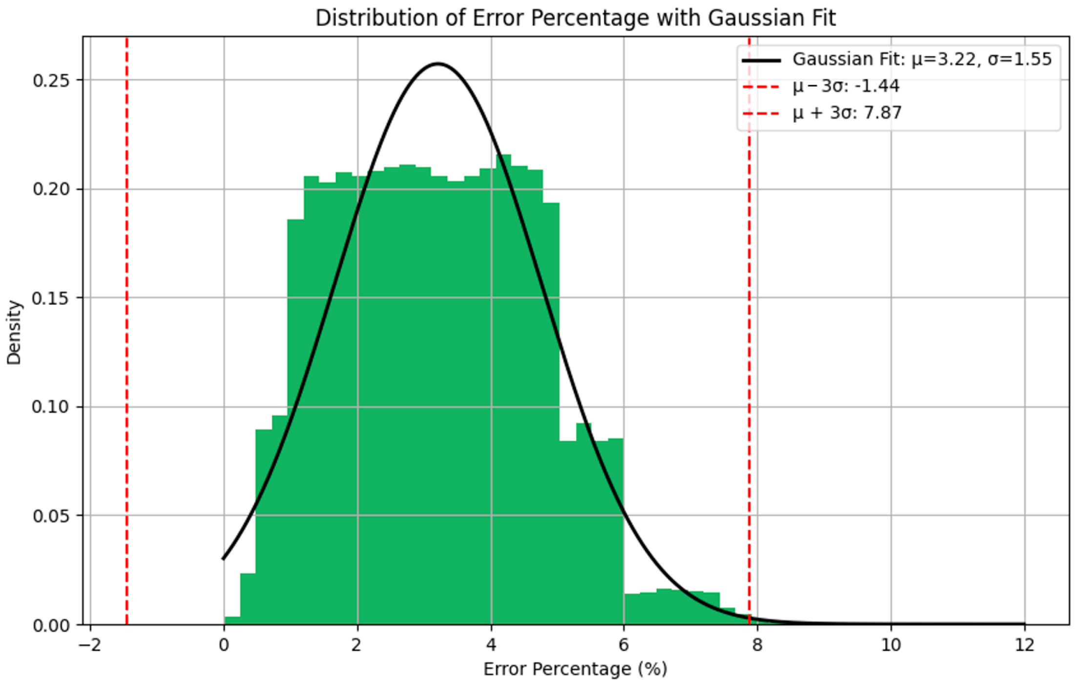
• External heat flux calculations reveal significant disparities in thermal flux density between sunlit and shadowed instrument surfaces, with a mean error of 3.22% compared to COMSOL Multiphysics 6.2^® simulations. This can be used as a key input for subsequent temperature field calculations.
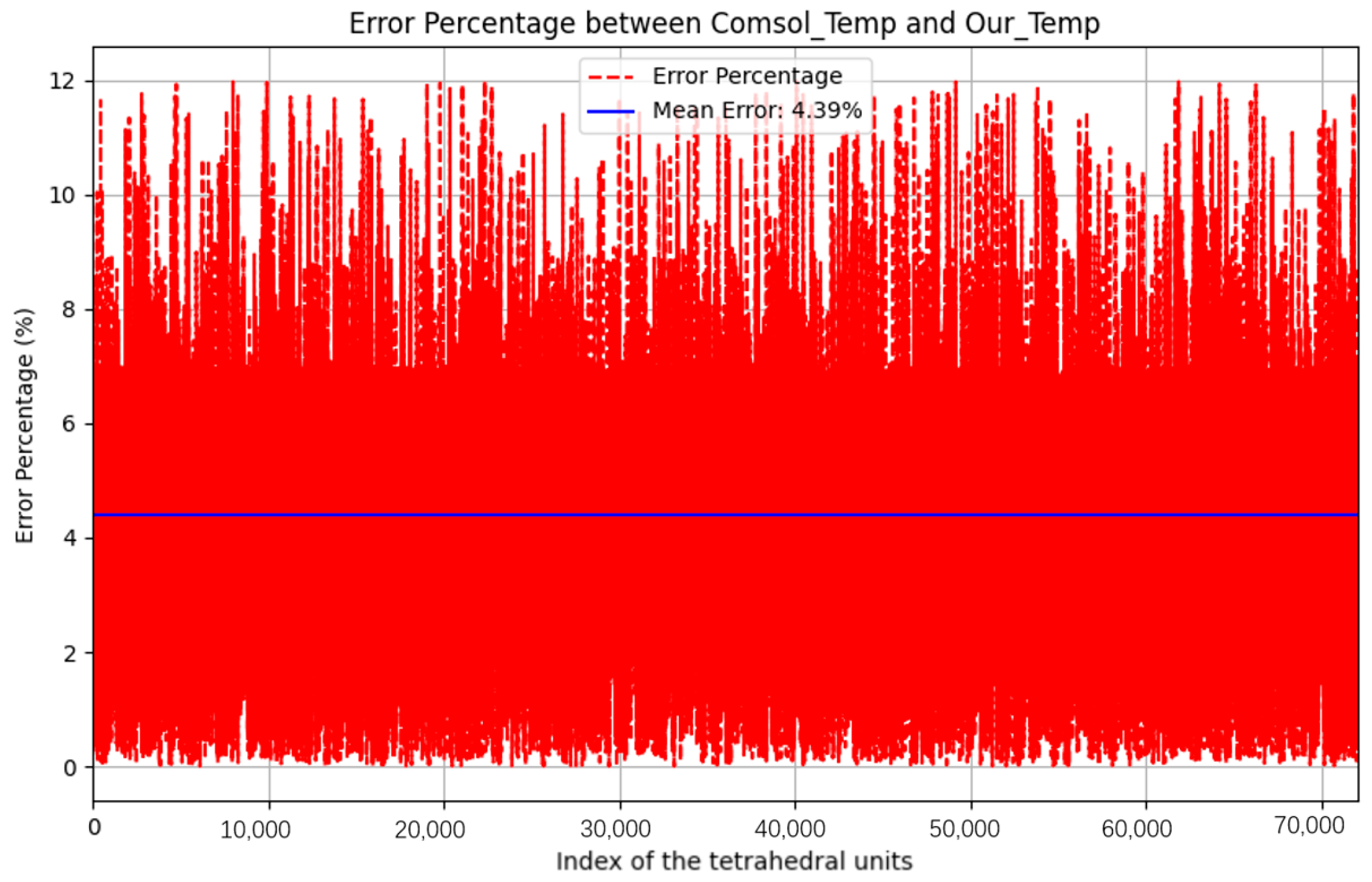
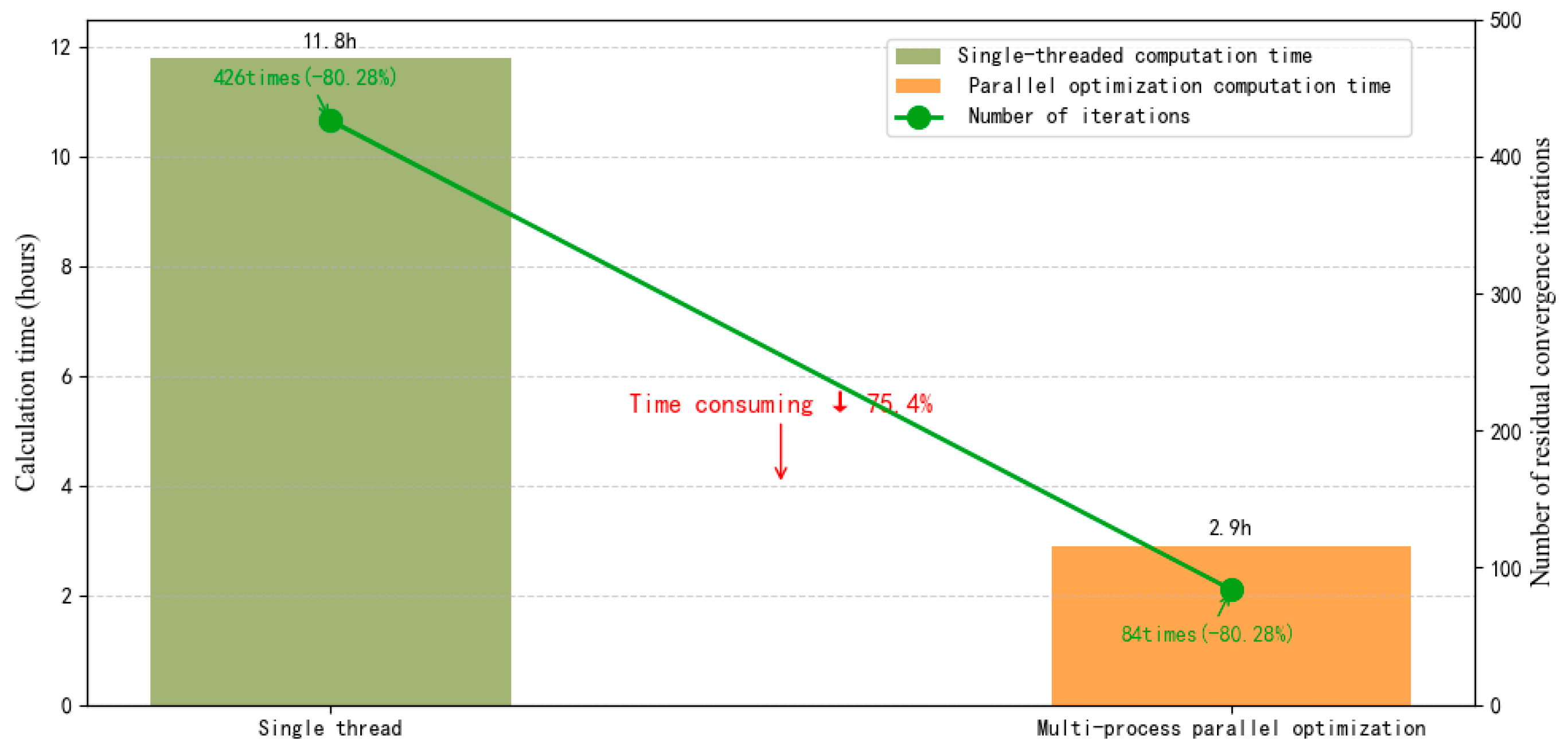
• For temperature field solutions, LU decomposition-based parallel optimization reduces computational time from 11.8 h to 2.9 h, yielding steady-state temperature distributions ranging from −45 °C to 51.13 °C. Computational errors relative to COMSOL simulations follow a Gaussian distribution (μ = 4.39%, σ = 1.66%), satisfying engineering accuracy requirements.
• Under the influence of temperature effects, the performance of the PUIA after thermal deformation is analyzed in this paper. Compared with the simulation results before thermal deformation, the ion energy resolution, angular resolution, detection field of view, geometric factor, and mass spectrometry resolution of the PUIA after thermal deformation are not more than 7.2%.
• This research reveals the thermo-mechanical coupling effect of the PUIA in the deep-space thermal environment. Through the high-precision external heat flow method and the parallel algorithm based on LU decomposition, the calculation efficiency of the temperature field was increased by 75%, and the calculation of the thermal deformation caused by the temperature layer was completed.

This research systematically quantifies temperature effects on PUIA performance in deep-space environments, and the proposed methodology could provide technical support for optimizing on-orbit thermal management strategies. Following mission launch and during in-orbit operation, further validation experiments will be conducted to refine the methodologies, thereby enabling their application to a broader range of space exploration missions. Future work will focus on developing multiphysics simulation methods (e.g., thermal–electromagnetic) to quantify charging effects on retarding potential analyzer voltage stability and investigate performance under diverse space environmental conditions.

References

1. Yang, Y.; Lei, N.; Li, S.; Zhang, J. Infrared radiation properties of a satellite on the basis of 3D reconstruction. Appl. Opt. 2024, 63, 721–729. [Google Scholar] [CrossRef] [PubMed]
2. Semena, N.P. The Importance of Thermal Modes of Astrophysical Instruments in Solving Problems of Extra-Atmospheric Astronomy. Cosm. Res. 2018, 56, 293–305. [Google Scholar] [CrossRef]
3. Zhang, J.Y.; Wang, H.Y.; Zhang, C.M.; Yang, J.; Liang, X.; Gao, M.; Wang, J.; Cui, X.; Peng, W. Thermal Control Design and Simulation Calculation of the Alpha Particle X-ray Spectrometer. Chin. J. Space Sci. 2013, 33, 672–677. [Google Scholar] [CrossRef]
4. Seo, H.S.; Rhee, J.; Han, E.S.; Kim, I.-S. Thermal failure of the LM117 regulator under harsh space thermal environments. Aerosp. Sci. Technol. 2013, 27, 49–56. [Google Scholar] [CrossRef]
5. Gao, T.F.; Kong, L.G.; Su, B.; Zhang, A. Design and simulation of the detector for outer heliosphere pickup ions. J. Beijing Univ. Aeronaut. Astronaut. 2021, 49, 367–377. [Google Scholar] [CrossRef]
6. Cao, Y.; Zhang, Y.Z.; Peng, X.D.; Xue, C.B.; Su, B. A Comparative Analysis of Performance Simulation for PUI Detectors Based on Traditional Probability Model and the Vasyliunas and Siscoe Model. Sensors 2024, 24, 6233. [Google Scholar] [CrossRef] [PubMed]
7. Wu, Y.H.; Chen, L.H.; Li, H.; Li, S.J.; Yang, Y.T. Computation of external heat fluxes on space camera with attitude change in geostationary orbit. Infrared Laser Eng. 2019, 48, 284–292. [Google Scholar] [CrossRef]
8. Freire, P.C.; Kramer, M.; Lyne, A.G. Determination of the orbital parameters of binary pulsars. Mon. Not. R. Astron. Soc. 2001, 322, 885–890. [Google Scholar] [CrossRef]
9. Lee, S.H.; Eman, K.F.; Wu, S.M. Trajectory control in the world coordinate system by an adaptive forecasting algorithm. Int. J. Prod. Res. 1989, 27, 451–461. [Google Scholar] [CrossRef]
10. Geng, Y. The Design and Implementation of External Heat Flux Calculation Software Based on the 3D Structure of the Satellite. Master’s Thesis, University of Chinese Academy of Sciences, Beijing, China, 2012. [Google Scholar]
11. Li, Y.Z.; Ning, X.W.; Wang, X.M.; Shi, X.B.; Zhuang, D.M.; Wang, J. Simulating Analysis of Nano-satellite’s Orbital Thermal Environment. J. Syst. Simul. 2007, 19, 4. [Google Scholar] [CrossRef]
12. Zheng, Y.H.; Ganushkina, N.Y.; Jiggens, P.; Jun, I.; Meier, M.; Minow, J.I.; O’Brien, T.P.; Pitchford, D.; Shprits, Y.; Tobiska, W.K.; et al. Space radiation and plasma effects on satellites and aviation: Quantities and metrics for tracking performance of space weather environment models. Space Weather 2019, 17, 1384–1403. [Google Scholar] [CrossRef] [PubMed]
13. Anh, N.D.; Hieu, N.N.; Chung, P.N.; Anh, N.T. Thermal radiation analysis for small satellites with single-node model using techniques of equivalent linearization. Appl. Therm. Eng. 2016, 94, 607–614. [Google Scholar] [CrossRef]
14. Li, P.; Cheng, H.E.; Qin, W.B. Numerical simulation of temperature field in solar arrays of spacecraft in low earth orbit. Numer. Heat Transf. Part A Appl. 2006, 49, 803–820. [Google Scholar] [CrossRef]
15. Wang, L. Research on Thermal-Structural Analysis of in-Orbit Parabolidal Satellite Antenna. Master’s Thesis, Harbin Institute of Technology, Harbin, China, 2011. [Google Scholar]
16. Shen, W.T.; Zhu, D.Q.; Cai, G.B. Calculation of Temperature Field and Infrared Radiation Characteristics of Midcourse Ballistic Target. J. Astronaut. 2010, 31, 2210–2217. [Google Scholar] [CrossRef]
17. Perret, W.; Schwenk, C.; Rethmeier, M. Comparison of analytical and numerical welding temperature field calculation. Comput. Mater. Sci. 2010, 47, 1005–1015. [Google Scholar] [CrossRef]
18. Chen, X.D.; Yang, J.; Zhao, X.D.; Fang, X.Q. The Status and Development of Finite Element Method. Manuf. Inf. Eng. China 2010, 39, 6–8. Available online: https://qikan.cqvip.com/Qikan/Article/Detail?id=34126107 (accessed on 2 April 2025).
19. Zhang, J.Q.; Yu, B.; Song, C.M. The latest progress in research on the scaled boundary finite element method. Chin. J. Appl. Mech. 2022, 39, 1038–1054. Available online: https://www.researchgate.net/publication/366739588_bilibianjieyouxianyuanfadezuixinyanjiujinzhan_The_latest_progress_in_research_on_the_scaled_boundary_finite_element_method (accessed on 2 April 2025).
20. Du, T.S.; Tan, T.G. Numerical Analysis and Experiments, 2nd ed.; Science Press: Beijing, China, 2012; ISBN 9787030356345. [Google Scholar]
21. Ding, L.J.; Cheng, Q.Y. Numerical Calculation Methods, 2nd ed.; Beijing Institute of Technology Press: Beijing, China, 2005; ISBN 9787810453172. [Google Scholar]
22. COMSOL. Newly released COMSOL Multiphysics~6.2 version. Electr. Age 2023, 18–19. Available online: https://d.wanfangdata.com.cn/periodical/dqsd202312005 (accessed on 2 April 2025).
23. Zhang, D.M. Research on Temperature Characteristics of Optical Antenna for Satellite Optical Communication Terminal. Master’s Thesis, Harbin Institute of Technology, Harbin, China, 2011. [Google Scholar]
24. Zienkiewicz, O.C.; Taylor, R.L.; Zhu, J.Z. The Finite Element Method: Its Basis and Fundamentals, 7th ed.; Butterworth-Heinemann: Oxford, UK, 2013. [Google Scholar] [CrossRef]
25. Han, J.; Dai, Q.; Zhao, Y.L.; Li, G.M. Study on Fatigue Performance of 7075-T651 Alum inum Alloys. J. Aeronaut. Mater. 2010, 30, 92–96. Available online: https://kns.cnki.net/kcms2/article/abstract?v=EKYfHJ8l29hQrTZKDauIiJmRJxe6s0xrJpceD-VgmT6-5hj4NedKtEpL__5knwWRmA70yBz6Sp6eTF8gKse7-t9it4KeZO4K7t94-uvD5Nr-0etxBtIj75dL4eNamC2--9UYHnogY2Wde3QN-zLaQqrXS84Bo5hLej7MUpq-NJuQ5GpHoqfprA==&uniplatform=NZKPT&language=CHS (accessed on 2 April 2025).
26. Mínguez, J.M.; Vogwell, J. Fatigue life of an aerospace aluminum alloy subjected to cold expansion and a cyclic temperature regime. Eng. Fail. Anal. 2006, 13, 997–1004. [Google Scholar] [CrossRef]
Figure 1. Geocentric equatorial inertial coordinate system.
Aerospace 12 00388 g001
Figure 2. Spacecraft payload orbital coordinate system.
Aerospace 12 00388 g002
Figure 3. Flow chart of the impact analysis of temperature effects on the performance of the PUIA.
Aerospace 12 00388 g003
Figure 4. Flow chart of payload external heat flow calculation.
Aerospace 12 00388 g004
Figure 5. Schematic diagram of occlusion relationship judgment.
Aerospace 12 00388 g005
Figure 6. Solar radiation.
Aerospace 12 00388 g006
Figure 7. Flow chart of payload temperature field calculation.
Aerospace 12 00388 g007
Figure 8. PUIA partitioning structure diagram.
Aerospace 12 00388 g008
Figure 9. Multiprocessing library composition diagram.
Aerospace 12 00388 g009
Figure 10. Flowchart of the multiprocessing algorithm using the multiprocessing library.
Aerospace 12 00388 g010
Figure 11. Flowchart of thermoelastic deformation calculation.
Aerospace 12 00388 g011
Figure 12. The results of PUIA tetrahedral partitioning.
Aerospace 12 00388 g012
Figure 13. External heat flow distribution of the PUIA: (a) simulation results of the method proposed above and (b) COMSOL results.
Aerospace 12 00388 g013
Figure 14. The error percentage of the external heat flow calculated using the method presented in this paper and COMSOL.
Aerospace 12 00388 g014
Figure 15. Gaussian fitting distribution of external heat flow error percentage.
Aerospace 12 00388 g015
Figure 16. Temperature field distribution of the PUIA: (a) simulation results of the method proposed above and (b) COMSOL results.
Aerospace 12 00388 g016
Figure 17. The convergence graph of the PUIA temperature field numerical solution provided by COMSOL.
Aerospace 12 00388 g017
Figure 18. The error percentage of the temperature field calculated using the method presented in this paper and COMSOL.
Aerospace 12 00388 g018
Figure 19. Gaussian fitting distribution of temperature field error percentage.
Aerospace 12 00388 g019
Figure 20. Grid independence test result graph.
Aerospace 12 00388 g020
Figure 21. Algorithm optimization effect comparison (calculation time and number of iterations).
Aerospace 12 00388 g021
Figure 22. Structural diagram of the PUIA after thermal deformation.
Aerospace 12 00388 g022
Figure 23. Diagram and results of performance indicators analyzed after thermal deformation: (a) differential curve of the ion counting rate under retarding potential analyzer (RPA) voltage; (b) pitch angle center angle fitting curve; (c) ESA simulation ion energy; (d) influence of temperature effect on the performance of the PUIA.
Aerospace 12 00388 g023aAerospace 12 00388 g023b