Abstract
Developing spacecraft for efficient aerocapture missions demands managing extreme aerothermal environments, precise controls, and atmospheric uncertainties. Successful designs must integrate vehicle airframe considerations with trajectory planning, adhering to launcher dimension constraints and ensuring robustness against atmospheric and insertion uncertainties. To advance robust multi-objective optimization in this field, a new framework is presented, designed to rapidly analyze and optimize non-thrusting, fixed angle-of-attack aerocapture-capable spacecraft and their trajectories. The framework employs a three-degree-of-freedom atmospheric flight dynamics model incorporating planet-specific characteristics. Aerothermal effects are approximated using established Sutton–Graves, Tauber–Sutton, and Stefan–Boltzmann relations. The framework computes the resulting post-atmospheric pass orbit using an orbital element determination algorithm to estimate fuel requirements for orbital corrective maneuvers. A novel algorithm that consolidates multiple objective functions into a unified cost function is presented and demonstrated to achieve superior optima with computational efficiency compared to traditional multi-objective optimization approaches. Numerical examples demonstrate the methodology’s effectiveness and computational cost at optimizing terrestrial and Martian aerocapture maneuvers for minimum fuel, heat loads, peak heat transfers, and an overall optimal trajectory, including volumetric considerations.
1. Introduction
A critical step in planetary exploration is the transition of a spacecraft from a hyperbolic trajectory to a closed orbit around a target planet. Conventional orbit insertion relies on high-thrust chemical propulsion systems, which require substantial propellant reserves, thereby limiting the available payload mass. Since the early 2000s, the adoption of electric propulsion for orbital insertion has grown significantly. Due to its extreme efficiency, its use for deep space missions and attitude control has rapidly increased. However, despite its benefits, electric propulsion has rarely been employed for full orbital capture. Instead, many missions have utilized electric propulsion primarily for station-keeping and proximity operations rather than achieving a bound orbit. To date, only three missions—SMART-1 [1], Dawn [2,3], and Psyche [4]—rely primarily on electric propulsion for orbital insertion, leveraging continuous low-thrust trajectories over extended durations.
Aerocapture offers a compelling alternative to conventional propulsive orbit insertion, utilizing atmospheric drag to decelerate the spacecraft and eliminating the need for large propellant reserves. This approach has the potential to significantly enhance payload capacity. Since its initial introduction [5], the feasibility and implementation of aerocapture have been extensively studied in the literature [6,7,8,9]. A comparative study assessing the relative risks of propulsive capture, aerobraking, and aerocapture concluded that the reliability of these three strategies differed only marginally [6]. This was largely because nearly all subsystems required for aerocapture had already demonstrated flight heritage and operational reliability in previous missions.
Recent studies demonstrate that NASA is technologically equipped to implement aerocapture Titan, Mars, and Venus [8,9]. These reports state that a dedicated flight demonstration mission is unnecessary, as several aeroassisted techniques—each presenting greater challenges than aerocapture—have been successfully executed. These include the skip-entry maneuver employed by the Soviet Zond [10], the Chinese Chang’e 5-T1 [11], the Apollo 4 and 6 missions [12], and the hypersonic aeromaneuvering task performed by the MSL [13], which all exemplify such achievements. Nonetheless, space exploration mission planners remain reluctant to adopt aerocapture due to flight-day uncertainties, including variations in atmospheric density and adverse meteorological conditions.
Recent optimization efforts in this field [14,15,16,17,18,19,20,21] have centered on the pursuit of efficient trans-atmospheric trajectories through meticulous manipulation of drag and lift forces to achieve an optimal aerocapture or reentry maneuver. Recent years have witnessed a push towards enhancing aerocapture technology through drag modulation (DM) techniques, particularly with the exploration of non-rigid aeroshell concepts such as HIAD and ADEPT [22]. These methods allow control over the spacecraft’s ballistic coefficient () by manipulating either the reference area or the drag coefficient (). The manipulation of these quantities can be performed either via continuous strategies or discrete events. However, certain technical challenges remain, particularly those associated with jettison or deployment events during hypersonic flight [23]. In contrast, lift modulation, which has been successfully demonstrated in missions such as Apollo, MSL, and the Space Shuttle, relies on sophisticated avionics algorithms and control systems to enable continuous bank angle modulation. Despite the complexities associated with this technique, it remains better understood and established than DM techniques. Optimal aerocapture problems have often overlooked the complex engineering challenges in effecting control over these parameters. Furthermore, the influence of aerodynamic control on the resulting captured orbit is limited, and its nature is highly dependent upon the spacecraft’s state at the atmospheric interface . Consequently, optimizing the atmospheric trajectory yields only incremental benefits to the overall mission, primarily impacting atmospheric phenomena such as heat loads.
Several optimization strategies for aerocapture trajectories avoid the continuous modulation of control variables during the atmospheric pass, instead relying on low-thrust maneuvers to guide the spacecraft to its desired operational orbit after the atmospheric phase. Giordano and Topputo [24] demonstrated this approach through ballistic capture. Their technique exploited gravitational interactions with multiple celestial bodies at the same time, allowing the Sun’s gravity to accelerate the spacecraft and naturally raise its periapsis, eliminating the need for a periapsis raise burn. Additionally, Fornari and Pontani [25] explored the impact of uncertainties in initial conditions and atmospheric density on aerocapture mission success, as well as the use of nonlinear orbit correction maneuvers to improve robustness. Their statistical analysis showed a high likelihood of three unfavorable outcomes—escape, near-capture, and destructive entry—necessitating distinct corrective maneuvers to ensure a successful trajectory. In a separate study, Gochenaur et al. [26] examined the feasibility of using lift vectoring for orbital plane rotations. While their focus was on assessing the maneuver’s viability rather than its practical implementation within an optimization framework, their work laid the foundation for future applications, as plane change maneuvers are known to be highly fuel-intensive.
However, because these studies assume specific vehicle geometries and initial conditions at the atmospheric interface, they are not well suited for preliminary mission design and planning applications. Given the multidisciplinary nature of such missions, an optimization framework must account for both the initial conditions—linked to the injection orbit—and vehicle sizing—determined by mission requirements—to provide planners with an optimal and viable preliminary solution. The AMAT framework [27], built on previous work by Girija [28], is a Python-based tool designed to aid in the design and sizing of re-entry vehicles for aeroassisted trajectories, making it particularly useful for preliminary mission planning. However, its primary focus is on trade-off analysis rather than design optimization. An example of a more suitable algorithm for preliminary design is the framework developed by Armellin and Lavagna [29], which enables a detailed analysis of the interplay between vehicle shape, trajectory control, and thermal protection system design. However, this framework assumes that the orbital plane achieved as the vehicle exits the atmosphere matches the target orbit plane, thereby yielding the target entry flight path angle (EFPA). However, that study overlooks uncertainties in EFPA and atmospheric density, meaning the entire interplanetary injection trajectory is designed without accounting for these critical uncertainties, which play a crucial role in determining mission success [25]. The approach proposed by Hanninen et al. [30] shares these same limitations.
Additionally, current strategies often employ multi-objective optimization (MOO) [14,15,16,17,29] for optimal re-entry trajectory problems, presenting numerical and decision-making challenges. MOO involves navigating a multi-dimensional objective space, resulting in trade-offs between objectives. The exploration of vast potential solutions and the non-convex and irregular Pareto front further complicates optimal solution searches. Selecting a single solution from a multitude of trade-offs involves considering subjective preferences, priorities, and uncertainty, requiring informed judgment, which can be challenging for algorithms due to ambiguous decision-making criteria.
In light of these multifaceted challenges—including the difficulty of continuously controlling lift and drag, uncertainties in EFPA, scattering of atmospheric densities, and the limitations of frameworks that impose fixed geometry or insertion trajectories—we propose a novel framework that supports the rapid preliminary design and optimization of aerocapture missions without the restrictive assumptions on vehicle geometry and insertion trajectory. Developed in MATLAB 2023a, the Determination of Aerocapture Successful Trajectories and Robust Optimization (D-ASTRO) algorithm is an efficient and robust tool designed for rapid analysis and optimization of generic aerocapture missions. Its unique capability lies in its ability to optimize the insertion trajectory and sizing of fixed angle-of-attack trajectories for aerocapture-capable spacecraft, while accounting for critical uncertainties. By requiring only minimal aeroshell information and mission parameters, D-ASTRO employs a nonlinear, single-objective constrained optimization strategy to identify optimal values for the flight path angle () at the AI and the fixed ballistic coefficient () of the aeroshell.
The paper is structured as follows: Section 2 introduces the concept of the aerocapture corridor. The optimization problem, along with novel objective functions and performance metrics, is discussed in Section 3. Section 4 focuses on the pipeline of the algorithm and the novel methodology used to rapidly compute the aerocapture corridor boundaries. Followed by the modeling considerations in Section 5. Finally, Section 6 presents the algorithm’s numerical stability and convergence properties applied to a typical Martian aerocapture mission test case, with the computational considerations and performance of D-ASTRO explored in Section 7.
2. Aerocapture Corridor
Without employing lift or drag modulation, the flight path angle at the AI and primarily govern the vehicle dynamics during the atmospheric pass, ultimately determining the success of the aerocapture maneuver. The aerocapture corridor defines the range of and values that result in a successful maneuver, that is, any atmospheric pass that results in a bounded orbit with an apoapsis greater than a specified altitude. The lower boundary is reached when excessive drag causes the spacecraft to descend to the surface, a condition which is readily determined by checking when the altitude along the trajectory reaches zero. In contrast, the upper boundary is defined by the condition where insufficient energy is dissipated, leaving the vehicle in a hyperbolic orbit. This is determined by the eccentricity of the orbit after the atmospheric pass, where indicates a closed orbit. Notably, trajectories exceeding the upper boundary may still be considered optimal if they significantly decelerate the spacecraft, although they necessitate a subsequent propulsive burn to reduce orbital energy, resulting in an aerobraking maneuver.
Figure 1 compares the aerocapture corridors for ballistic and lifting re-entry profiles of a spacecraft approaching Mars with a hyperbolic excess velocity, , of 3.5 . The maneuver’s success is represented by green hashing in Figure 1. These contours illustrate the intricate relationship among , , and the lift-to-drag ratio necessary for successful maneuver. A lifting re-entry profile provides a more favorable corridor, reducing sensitivity to precise insertion attitudes. While D-ASTRO supports various re-entry profiles, this study focused on non-zero profiles for Martian aerocapture, utilizing a fixed value of 0.2. This choice aligns with the design characteristics of heritage Martian re-entry vehicles [24,31].
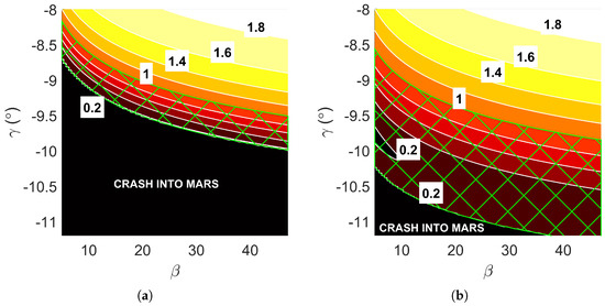
Figure 1.
Example of Martian aerocapture corridors with post-atmospheric pass orbital eccentricity contours: (a) ballistic re-entry profile, ; (b) lifted re-entry profile, .
Uncertainties in atmospheric properties significantly influence the width of the aerocapture corridor. Variations in atmospheric density lead to changes in drag forces, causing the spacecraft to dissipate energy differently than expected. Near the aerocapture boundaries, even minor density fluctuations can result in maneuver failure, leading to either a hyperbolic orbit or surface collision. Two corridors are computed to establish a robust corridor: one with reduced atmospheric density and another with increased density. The “robust” aerocapture corridor represents the intersection of these two, resulting in a narrowed corridor. These corridors are illustrated in Figure 2, depicting terrestrial and Martian corridors for various inbound , where the green and yellow regions represent the robust and non-robust corridors.
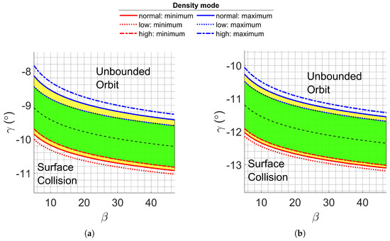
Figure 2.
Martian and terrestrial aerocapture corridors for multiple hyperbolic excess velocities, . The polynomial fits for low, mean, and high-density corridor boundaries are shown: (a) Martian aerocapture corridor with ; (b) Martian aerocapture corridor with .
3. Optimal Aerocapture Maneuver via Parameter Optimization
Multiple approaches can be taken to optimize an aerocapture trajectory. However, we focused on the optimization of design parameters and which yielded an optimal aerocapture, or aeroassisted, trajectory. Determining these two parameters allows mission planners to identify the most suitable interplanetary orbit, sizing of the spacecraft’s aeroshell, and structural design of the heat shield to ensure an optimal trajectory.
3.1. Formulation of Optimization Problem
The optimal aerocapture corridor problem is a constrained nonlinear optimization problem of the form:
where f represents the objective function, and and are functions of that define the upper and lower boundaries of the aerocapture corridor. The vector comprises selected performance indices.
Insertion inaccuracies arising from navigation and modeling errors can lead to significant deviations from the intended atmospheric insertion coordinates. Deviating from the intended leads to different atmospheric trajectories, impacting the maneuver’s optimality and sometimes its success. To account for this, an expected insertion inaccuracy is incorporated as , which narrows the aerocapture corridor to ensure mission success is robust to insertion inaccuracies.
Insertion inaccuracies become particularly critical when the optimal trajectory approaches the lower boundary of the aerocapture corridor, as even minor deviations can result in excessively deep atmospheric dives that demand prohibitively high thrust levels to ensure success. Conversely, inaccuracies in trajectories close to the upper boundary are easier to correct, as these lead to an aerobraking maneuver, although a propulsive capture maneuver is required.
3.2. Performance Indices
This section introduces a series of typically used performance metrics for re-entry trajectories.
3.2.1. Thermal Environment
The corresponding aerocapture trajectory is computed for every candidate point, and the profile is available. Hence, is computed by locating the maximum value in the profile and Q by using Equation (2):
where is the total duration of the atmospheric flight.
3.2.2. Volumetric Constraints
To address fairing constraints and current technological limitations, this optimization process aims to minimize the volume of the aeroshell by reducing the “equivalent axisymmetric aeroshell radius”, , computed by rearranging Equation (3). This metric is preferred because it can represent any aeroshell configuration, from axisymmetric to complex high lift-to-drag designs, as long as and are known.
3.2.3. Orbital Corrective Maneuver
represents the fuel needed to adjust the post-atmospheric pass orbit to the predetermined target orbit. In reality, each candidate trajectory will have its unique optimal orbital corrective maneuver composed of complex transfers. To simplify comparisons between all candidate trajectories, trivial orbit transfers are used. These include two-impulse Hohmann transfers to raise the orbit’s periapsis and match the desired target orbital eccentricity. In addition, a plane change burn at the apoapsis is assumed to match the target orbital inclination. The required can be computed using Equation (4):
where a is the semi-major axis of the orbit and subscripts “i” and “t” denote the quantity evaluated at the post-atmospheric pass orbit (determined at AE) and the target operational orbit, respectively.
3.3. Single-Objective Function Optimization
This paper considered two formulations of optimization Problem 1. The first strategy is the most widely employed multi-objective optimization (MOO), where , and a novel single-objective optimization formulation is presented, where .
MOO is the preferred approach for re-entry trajectory optimization, addressing problems with multiple conflicting criteria that cannot be combined into a single objective. However, MOO methods face challenges, including non-unique optimal solutions and subjective decision-making. Additionally, achieving both convergence and diversity—how close and spread the candidate solutions are relative to the Pareto front—is complex. Consequently, a new optimization problem may need to be formulated to address these issues and improve the performance of the MOO process.
This paper opted to embed the weighting function in a single-objective cost function to enable the use of traditional gradient descent (GD) methods to solve the problem. The proposed objective function utilized the weighted least squares (WLS) approach and is presented below.
where is the weight vector that includes the biases of each performance index, and the definition of follows.
To combine multiple performance metrics into a single-objective function, feature scaling was applied prior to computing the weighted least squares, ensuring all metrics were on a comparable scale. For instance, Q and differ by five to seven orders of magnitude. Unlike the conventional use of feature scaling—typically employed to expedite the convergence of gradient descent algorithms—this normalization method was specifically implemented to preserve the relative weightings of the performance indices. By rescaling these indices to values between zero and one, via Equation (6), each metric’s contribution to the objective function was consistent with their weighting.
where and represent the upper and lower bounds of property . To perform accurate normalization when no constraints are imposed on the performance metrics, it is essential to understand the range of possible values each feature can take. However, computing this range can be challenging, and an approximate procedure for this is explained in Section 4. When constraints are applied to the performance metrics, the upper and lower bounds of the constraint can replace and . If strict enforcement of these constraints is required—though this is typically unrealistic during the preliminary design phase—barrier functions should be introduced.
4. The D-ASTRO Framework
D-ASTRO distinguishes itself through its pre-optimization phase, where the two-dimensional space spanned by and is studied to apply appropriate feature normalization and to implement a novel method of handling the nonlinear constraints introduced by and . The strategy used to find the optimal sizing of the spacecraft and corresponding optimal interplanetary orbit is defined as follows:
- (1)
- A user-specified range is sampled with seven linearly spaced points, including the upper and lower limits.
- (2)
- At each , a binary search determines the lower and upper corridor boundary values, and , respectively.
- (3)
- Normalization quantities , , , , , , , and can be computed:
- (a)
- For unconstrained performance metrics, these values have already been computed when and were devised. Section 4.1 explains how this is performed.
- (b)
- For constrained performance metrics, the upper and lower bounds of the constraint can replace and .
- (4)
- Sixth-order polynomials are fitted to and with to obtain a one-to-one relationship. This process is explored in Section 4.2.
- (5)
- After computing normalization quantities and polynomial fits, MATLAB’s fmincon optimizer is used, employing sequential quadratic programming with an active set strategy, as described by Gill et al. [32].
The Martian robust aerocapture corridor and polynomial fits for an injection orbit with are shown in Figure 3, with the normalization values listed in Table 1.
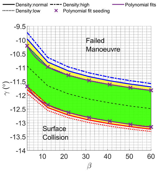
Figure 3.
Coarse robust Martian aerocapture corridor for used to compute normalization quantities listed in Table 1 and sixth-degree polynomial fits.

Table 1.
Minimum and maximum values of considered metrics for a Martian aerocapture corridor for .
4.1. Computation of Normalization Quantities
As discussed in Section 3.3, computing the extremal values of the performance metrics in is crucial for casting the optimization problem into an SOO form. In the following, we investigate which and values may achieve these targets.
For volumetric constraints, the bounds are easily computed based on , with maximum and minimum volumes corresponding to the lower and upper limits of , respectively. Thermal metrics, such as , increase with deeper atmospheric entries, so reaches its maximum at the lower corridor boundary and upper limit, while the minimum occurs at the upper corridor boundary and lower limit. The same applies to Q, which is maximized for deeper entries. Determining the bounds of is more complex, as post-atmospheric trajectory eccentricities can span from 0 to 1 within the aerocapture corridor. If circularization and plane-change maneuvers are neglected, . Hence, we assign , while depends on the operational orbit and requires an assessment across the ’s.
This analysis focuses on identifying the maximum and minimum values within the corridor. While the optimizer can explore and values beyond those used for normalization, this discrepancy does not significantly impact the process. Normalization ensures that values remain on a similar scale, with values exceeding the estimated maximum normalized above 1 and smaller values becoming negative. However, the nonlinear constraints and enforce candidate points within the corridor, mitigating this issue.
4.2. Approximating Aerocapture Corridor Boundaries via Polynomial Fitting
The primary challenge in aerocapture optimization lies in handling the nonlinear constraints introduced by and in Problem 1. Current optimization techniques necessitate computing and at each internal candidate point, significantly increasing execution time despite efficient search algorithms. This is quantitatively characterized in Section 7.
Multiple Martian aerocapture corridors with various hyperbolic approach orbits were analyzed. Figure 2 illustrates two examined corridors. From this figure, it is evident that the upper and lower corridor boundaries exhibited an exponential trend over the considered range. Several candidate functions were considered to rapidly map to and , including exponential and polynomial curves.
Initial testing revealed the limitations of a primary exponential curve ( in Equation (7)), leading to the adoption of a second-degree exponential fit (), significantly enhancing predictive accuracy with error bounded by a Martian aerocapture. However, when terrestrial aerocapture was explored, the lower corridor boundary experienced a non-exponential-like trend, due to differing atmospheric structures of the planets at low altitudes. Hence, to expand the applicability of this technique to multiple celestial bodies, sixth-degree polynomial curves were examined due to the potential flat nature of some boundaries. As illustrated by Figure 4, the polynomial curves resulted in excellent predictive capabilities, exceeding the former’s accuracy. These observations were consistent for terrestrial aerocapture missions.
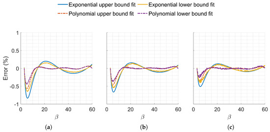
Figure 4.
Percentage error between finely discretized corridor limits (570 points) and computed values using exponential and polynomial constructed from 7 points. (a) Mars, = 1.0 . (b) Mars, = 3.0 . (c) Mars, = 6.0 .
Exploration into the minimum number of points required for accurate fitting demonstrated that the accuracy of the fits was very sensitive to the selected fitting points. Randomly selecting seven points within the interest range demonstrated poor fit accuracy, as illustrated by Figure A1. However, when the fitting points were evenly distributed across the range, both fits exhibited increased accuracy with fewer fitting points. Specifically, fitting the sixth-degree polynomial with seven linearly spaced points proved to capture boundaries accurately, resulting in superior approximations in flat boundaries. Figure 4 illustrates the error between the actual boundary and the proposed fits, comparing the second-degree exponential fit with the sixth-degree polynomial fit, both fitted with 7 linearly spaced points.
5. Modelling
5.1. Atmospheric Flight Dynamics
At the preliminary design stages of an aerocapture-capable spacecraft, key geometric parameters such as the inertia matrix, center of mass, and center of pressure are undefined, limiting the analysis of rotational kinematics during re-entry. Consequently, D-ASTRO employs a three-degree-of-freedom (three-DOF) model. The equations describing flight over a spherical planet in a planet-fixed reference frame are as follows [33]:
where r is the radial distance from the planet’s center to the vehicle, V is the planetocentric velocity, is the flight path angle, and are the longitude and latitude, respectively, and is the heading angle. Additionally, m denotes the spacecraft’s mass, L and D are the lift and drag forces, respectively, and and represent the planet’s gravitational parameter and rotational period of the planet, respectively. The atmosphere is assumed to be at rest with respect to the planet.
Let the trajectory state in Equation (8) be . The initial condition of is assumed to be user-specified and coincident with the atmospheric interface (AI).
5.2. Aerodynamic Model
Accurately approximating the aerodynamic coefficients, and , is essential for properly simulating the trans-atmospheric trajectory. These coefficients depend on the angle of attack, which, in reentry applications, varies with the Mach number. However, given the high velocity of this maneuver, the spacecraft operates in a fully hypersonic regime, where the Mach independence principle allows these coefficients to be treated as constant [34].
Nevertheless, at high altitudes, gas rarefaction effects can cause deviations from the Mach independence principle. To address this, D-ASTRO enables users to define and as functions of Mach number , Reynolds number , and Knudsen number , enhancing accuracy, as outlined in Equations (9) and (10):
where is the freestream density, and is the reference area of the aeroshell.
5.3. Aerothermal Model
To compute the heat flux, , and heat load, Q, of the trajectory in a simplistic manner, the thermal model focuses on stagnation-point aerothermal heating, as this is the expected peak heat transfer region of the aeroshell. Thus, the Sutton–Graves relation, Equation (11), approximates the convective stagnation-point heating [35]. Furthermore, D-ASTRO incorporates the Tauber–Sutton relations, Equation (12), to account for radiative heat transfer, , in cases where re-entry speeds are moderately high [36]:
where is the nose radius, k, C, a, and m are atmospheric-specific constants, and is an empirically determined function that is also planet-specific.
In cases where wall temperature is a concern, it is common practice to employ the radiative equilibrium approach to approximate the equilibrium wall temperature [37]. This technique assumes that the surface temperature rapidly rises until it reaches a value at which the surface rejects all the convective heat flux, and sometimes radiation heat fluxes due to high-temperature shock layers, by black body re-radiation, leading to an energy balance between total heating, , and re-radiation cooling, , calculated using the Stefan–Boltzmann law, Equation (13). is approximated by Equation (14):
where is the emissivity, and is the Boltzmann constant.
5.4. Martian Atmospheric Model
A reliable atmospheric model is essential for accurately calculating the vehicle’s aerodynamic forces and aerothermal heating during the aerocapture maneuver. This report investigated the Martian atmosphere, highlighting the specific model below.
Mars-GRAM [38] was employed to generate atmospheric data for Martian aerocapture maneuvers. A simplified table was generated from the extensive data available in the Mars-GRAM database, encompassing atmospheric variations concerning seasons, latitude and longitude positions, and numerous other variables. This table is based on a yearly average of equatorial properties at zero longitude. Additionally, a statistical analysis was conducted to obtain an accurate variation in atmospheric properties for , which encompasses 99.73% of cases.
5.5. Computation of Keplerian Orbital Elements
Determining orbital elements is crucial for characterizing a spacecraft’s orbit after an atmospheric pass. The resulting orbit determines the amount of fuel required to obtain the target operational orbit via corrective maneuvers. D-ASTRO employs an algorithm for computing the Keplerian orbital elements from the Cartesian state of the spacecraft [39].
6. Results and Analysis
A Martian aerocapture mission was considered to assess the robustness and convergence properties of the proposed optimization strategy. The Martian atmosphere was modeled using data from Mars GRAM 2010 [38], an engineering-level atmospheric tool developed for mission design applications. D-ASTRO requires multiple input parameters, including spacecraft preliminary properties, insertion conditions, and target operational orbit. These input quantities are provided in Table 2 and Table 3.
Table 2.
Martian aerocapture simulation parameters.
Table 3.
Target operational orbit.
The optimization algorithm was subjected to various initial conditions to assess its convergence properties. The range of considered initial conditions comprised extreme and random values both within and outside the aerocapture corridor, with some having limited physical meaning. Table 4 provides detailed information on the initial conditions used ( and ).
Table 4.
Initial conditions used.
6.1. Dependencies on Solver Initial Conditions
A bias vector assigning equal importance to all performance indices (denoted as ) was employed for this examination. In Figure 5, level lines of the cost function are depicted within and around the aerocapture corridor. The region delineated by magenta solid lines represents the aerocapture corridor, defined by the novel polynomial fit approach discussed in Section 4. The figure illustrates that the novel objective function formulation was well suited for gradient descent (GD) algorithms, as it had no visible sharp discontinuities. Notably, areas where aerocapture failed, such as surface collisions in the lower left corner of the figure, incurred high costs, expediting solution convergence.
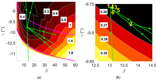
Figure 5.
Convergence property of D-ASTRO for overall optimal mission design, , with magenta lines delineating the boundaries of the aerocapture corridor. (a) Convergence of to . (b) Zoom into global minimum region.
Based on Table 5 and Figure 5, the problem’s minimum was near . While Case 2 indicated a slightly different optimal point (explored further in Section 6.2, the algorithm consistently converged to the global minimum, even with initial conditions lacking physical significance (e.g., Cases 1, 3, and 4). The strong convergence properties of D-ASTRO were further demonstrated by the similarity in trajectory profiles shown in Figure 6.
Table 5.
Convergence properties of optimization algorithm with different initial conditions.
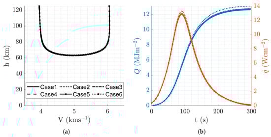
Figure 6.
Aerocapture trajectory profiles resulting from overall optimal mission design, . (a) Altitude vs. velocity. (b) Q and vs. time.
6.2. Minimum Fuel Mission Design
The adoption of an aerocapture maneuver is often motivated by a desire to minimize fuel requirements to achieve a desired operational orbit. The minimum fuel trajectory for the proposed case study could be identified by selecting . The same initial conditions as in the previous section were studied to assess convergence properties. Additionally, various target semi-major axis values, specifically km, km, and km, were analyzed to explore the behavior of the optimal solution.
As illustrated by the () cost contours in Figure 7 and the information in Table 6, this optimization problem yielded optima that were scattered over a broad range. However, it is crucial not to interpret this as a sign of poor convergence of D-ASTRO’s optimizer. Instead, understanding the underlying physics and formulation of the optimization problem is essential to justify this apparent discrepancy.
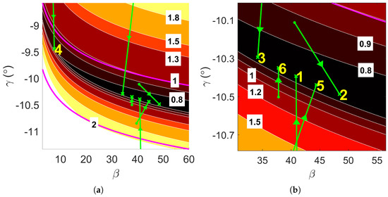
Figure 7.
Convergence property of D-ASTRO for minimum fuel mission design, , with magenta lines delineating the boundaries of the aerocapture corridor. (a) Convergence of to . (b) Zoom into global minimum region.
Table 6.
Optimal results for minimum fuel trajectory.
Figure 7 illustrates the presence of a low-cost valley in the cost function, directing the global minimum along a specific direction. The valley-like structure of the cost function characterized a typical aerocapture corridor, with the trough’s vertical position determined by the target a. Smaller values required deeper atmospheric entries, shifting the valley downward, while larger values led to shallower entries, moving it upward. The valley’s convex structure arose because one side required increasing orbital energy due to excessive energy depletion, while the other side required decreasing energy due to insufficient depletion. The valley in did not span the entire range; the increase in cost at low was linked to plane-change maneuvers. Figure 8 illustrates the contours without considering these maneuvers, revealing the anticipated valley that spans the entire range. The evolution of plane changes resulted from the forces acting on the spacecraft during atmospheric entry, which did not align with the orbital plane, thereby altering the inclination of the orbit’s plane.
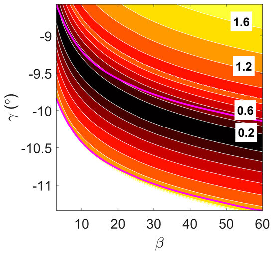
Figure 8.
contours for minimal fuel trajectory neglecting plane-change maneuvers, , and km.
To enhance convergence and mitigate the impact on other cases, the cost function for must be revised. Comparing contours in Figure 7a and Figure 8 shows that including significantly increased fuel requirement. Applying feature standardization to the total flattened the valley as , causing to dominate the problem. To address this, a potential solution is to decompose the into two components and apply separate standardizations.
Figure 9 depicts the optimal trajectory profiles. The extensive variation in both and resulted in a multitude of trajectories. It is crucial to emphasize that despite discrepancies in the h-v profiles shown in Figure 9a, they all converged to a similar velocity (V) at the atmospheric exit, thereby leading to approximately comparable values of . As anticipated, thermal quantities exhibited significant differences across all trajectories, reflecting the lack of assigned importance to these features in the optimization process.
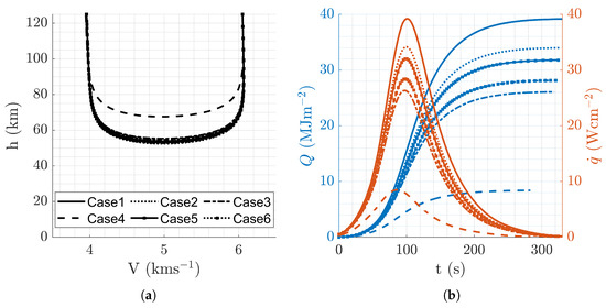
Figure 9.
Aerocapture trajectory profiles resulting from minimal fuel mission design, . (a) Altitude vs. velocity. (b) Q and vs. time.
6.3. Minimum Heat Load Mission Design
Ensuring mission success during re-entry requires equipping the spacecraft with a suitably robust thermal protective system (TPS). By minimizing the heat load experienced during the atmospheric trajectory, the TPS can be made more lightweight, allowing for an increased payload mass fraction.
As outlined by Equation (2), calculating stagnation-point heat loads requires complete trajectory knowledge. In practice, researchers often use Equation (15) for simplified heat load estimations during Entry, Descent, and Landing (EDL), based only on parameters like and at AI. Utilizing the Sutton–Graves model for and an exponential atmospheric model, Allen and Eggers [40] formulated the complete expression, suggesting that heat load could be reduced by minimizing and maximizing . This approach is later explored as a substitute for the current Q cost function for aerocapture missions.
Figure 10 illustrates the exploration of multiple initial conditions aimed at determining the optimal trajectory with the minimum heat load, revealing partially anticipated trends. Table 7 details the outcomes of the explored cases. All cases suggested values near the lower limit of feasible , consistent with Equation (15). However, only Case 1 aligned with the minimum of Q predicted by Equation (15), with at the lower boundary of feasibility, while other cases showed near the upper boundary.
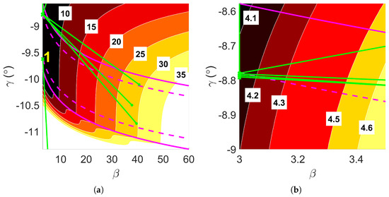
Figure 10.
Convergence property of D-ASTRO for minimum heat load mission design, , with magenta lines delineating the boundaries of the aerocapture corridor. (a) Convergence of to . (b) Zoom into global minimum region.
Table 7.
Optimal results for minimum heat load trajectory.
To investigate the disparity between the anticipated minimum of Equation (15) and the complete trajectory analysis, both heat loads were normalized with respect to their corresponding minima and maxima and are illustrated in Figure 11. This figure reveals differences in the contours of Q, particularly in the slopes with respect to ). The approximate expression in Equation (15) incorrectly suggested increments in Q with , whereas the complete trajectory analysis showed the opposite trend . This discrepancy stemmed from the assumption of an EDL trajectory made by Allen and Eggers [40].
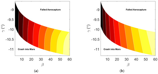
Figure 11.
Normalized heat load, . (a) Complete trajectory analysis. (b) Predicted by Equation (15).
Optimizing for the minimum Q highlighted the importance of the optimizer’s step tolerance in D-ASTRO’s robustness. Initially, fmincon’s default convergence criteria yielded reliable and consistent results, as demonstrated in Figure 5 and Figure 7. However, minimizing Q initially showed significant variations in due to the flat nature of the normalized Q () in the direction, with varying only slightly at the leftmost region of the corridor, of the order of . This was mitigated by reducing the function and step tolerance of the solver, causing D-ASTRO to identify the global minimum consistently, and in Case 1, a local minimum coincident with the feasibility boundary (see Figure A4). However, local minima could be avoided by selecting a reasonable initial condition. The decrement tolerance only benefited the convergence properties of the minimal Q trajectory, hindering the other problems with no changes in optimal trajectory for the other test cases. The resulting optimal trajectory profiles are shown in Figure 12, where the difference between the global and local minima trajectories can be seen.
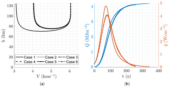
Figure 12.
Aerocapture trajectory profiles resulting from minimal heat load mission design, . (a) Altitude vs. velocity. (b) Q and vs. time.
6.4. Minimum Peak Heat Flux Trajectory
Similar to the parameter Q discussed earlier, the peak heat transfer rate plays a crucial role in determining the design specifications of the TPS. This metric underwent an independent optimization process to validate the underlying physics principles and the cost function employed.
The minimization of peak heat transfer demonstrated strong convergence properties, as shown in Figure 13 and Table 8, where multiple initial points converged to the same optima. The variation in convergence quality between Q and arose from the latter’s greater sensitivity to , illustrated by curved contours in Figure 13 versus the quasi-vertical contours of Figure 10. Figure 14 shows indistinguishable trajectory profiles, highlighting the optimizer’s robust convergence.
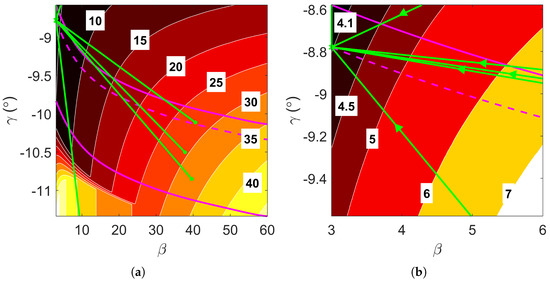
Figure 13.
Convergence property of D-ASTRO for minimum peak heating rate mission design, , with magenta lines delineating the boundaries of the aerocapture corridor. (a) Convergence of to . (b) Zoom into global minimum region.
Table 8.
Optimal results for minimal trajectory.
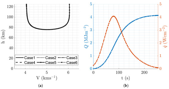
Figure 14.
Aerocapture trajectory profiles resulting from minimal peak heating rate mission design, . (a) Altitude vs. velocity. (b) Q and vs. time.
The results presented in Table 8 align with established expectations that smaller values of lead to reduced . However, the practical implementation of this solution is limited, as corresponds to an unfeasibly small value for a realistic mission, since unprecedented aeroshell surface areas (A) would be required to achieve that . However, introducing volumetric considerations in the optimization (non-zero first entry of ) would lead to a more realistic . The resulting optimal points of combining thermal loads and volumetric considerations is explored in the following Section, where and were considered.
6.5. Direct Comparison with MOO
This section compares D-ASTRO with a basic MOO algorithm using MATLAB’s fgoalattain optimizer. Multiple initial conditions were again tested to evaluate the solver’s convergence dynamics and stability. Figure 15 shows the convergence dynamics of both approaches, revealing significant disagreement in optimal solutions. Table 9 presents an additional comparison, incorporating data from Table 5.
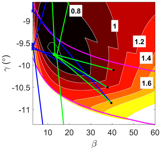
Figure 15.
Convergence property of MOO strategy for overall optimal mission design (blue) compared with D-ASTRO (green), , with magenta lines delineating the aerocapture boundaries.
Table 9.
Convergence properties of MOO algorithm and D-ASTRO for overall optimal trajectory.
From Figure 15, it is clear that the MOO optimizer experienced similar poor convergence in the leftmost region as D-ASTRO when only the minimal heat load trajectory was considered, yielding one of two possible solutions: a local or global minimum. The fact that the MOO strategy suffered from the same convergence issues as D-ASTRO, even when subjected to a wide range of initial conditions, suggested that the subjective decision-making inherent in the MOO strategy was not responsible for the disagreement in solutions. Ill conditioning of the optimization problem was not the reason behind that discrepancy, as the MOO strategy was conducted with and without D-ASTRO’s normalization technique and yielded identical results.
Further analysis revealed that the MOO strategy prioritized the optimization of Q and over and . As illustrated by Figure 10 and Figure 13, the heat load and peak heat rate cost functions exhibited a strong convex behavior in the direction, facilitating the rapid convergence of GD algorithms to the leftmost regions. In contrast, the volumetric consideration cost function experienced an inverse proportionality to , leading to rapid convergence to the rightmost regions. Finally, the cost function experienced a convex-like behavior in the direction, causing the optimality valley explored in Section 6.2.
The dynamics of the individual metrics cost contours indicated three convergence behaviors: one toward the left region of the corridor, another toward the rightmost regions, and a third toward the corridor’s center. We conclude that the MOO optimizer was attempting to globally optimize Q and , at the expense of , to later find the optimal in regions where Q and were quasi-globally optimal, as had a relatively low cost over the entire range. The resulting optimal trajectories are depicted in Figure 16.
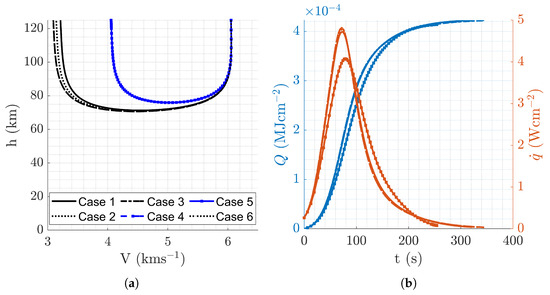
Figure 16.
Aerocapture trajectory profiles resulting from overall optimal mission design using MOO strategy, . (a) Altitude vs. velocity. (b) Q and vs. time.
For completeness, all optimal trajectory profiles presented in this paper are illustrated in Figure 17 to aid the comparison between the different optima.
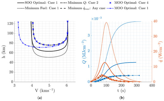
Figure 17.
Aerocapture trajectory profiles resulting from all optimal mission designs presented in this study. Initial conditions correspond to those that result in the lowest cost. (a) Altitude vs. velocity. (b) Q and vs. time.
7. Computational Performance and Considerations of D-ASTRO
This section examines the computational performance and considerations within the D-ASTRO framework. The analysis is divided into two parts: the first addresses the computational costs and considerations of the binary search algorithm used to compute the robust aerocapture corridor; the second evaluates the performance of the optimization process.
7.1. Dependency of Corridor Fits on Binary Search Tolerance
To balance accuracy and computational efficiency, a study was conducted to analyze how the accuracy of the computed corridor boundaries varied with different tolerance levels. To evaluate this, we computed the robust coarse aerocapture corridor depicted in Figure 3 using varying binary search tolerances. The overall accuracy of the resulting polynomial fits was assessed by calculating the Euclidean L-2 norm between actual corridor boundaries, computed from a finely discretized aerocapture corridor (570 points), and those computed using the fits. Figure 18 illustrates the evolution of polynomial fit accuracy for both lower and upper corridor boundaries over the considered range. Additionally, Figure 19 presents the cumulative accuracy via the Euclidean L-2 norm approach and the execution time of the corridor, examining a Martian aerocapture maneuver. This figure shows that the Euclidean norm reached a plateau at a tolerance of approximately in both scenarios, indicating that more accurate fits were not achievable with a further decrement in tolerance. Hence, for expedited solutions of D-ASTRO, a binary search tolerance of was selected as the optimal balance between computational efficiency and accuracy. For the selected tolerance level, 31 trajectory simulations were required to compute and , with the number of simulations being unaffected by the chosen .
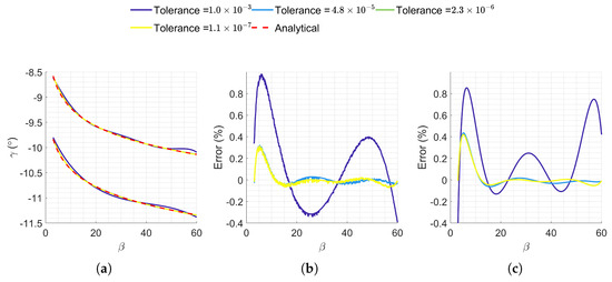
Figure 18.
Accuracy evolution of sixth-degree polynomial curves as a function of binary search tolerance used for computing fitting points. (a) Corridor boundaries. (b) Lower-bound fit. (c) Upper-bound fit.
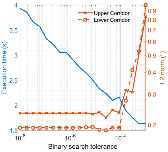
Figure 19.
Evolution of Euclidean L-2 norm of upper- and lower-boundary fits and execution time of robust coarse corridor for a Martian aerocapture with .
7.2. Execution Time of Optimizers
To evaluate the optimizers’ performance, 10 iterations of the optimization process were performed using a consistent initial guess ( and ) to minimize execution timing outliers. Various weightings () were also considered to further explore the convergence properties of MOO and D-ASTRO, highlighting the challenges of the multi-objective approach in optimizing these problems. Table 10 presents the execution time, number of function calls, time per function call, and the suggested optima for both methods. This table indicates a significant dependency of execution time on the weight vector and optimization strategy employed. However, the time required per function call was roughly consistent across all cases, with the MOO function requiring marginally less time than D-ASTRO’s. This difference arises from the distinct optimizers used, as fgoalattain and fmincon are fundamentally different algorithms.
Table 10.
Computational performance and suggested optima of D-ASTRO and MOO strategies with and for the Martian test case.
In general, D-ASTRO converged more quickly to the global optimum compared to the MOO strategy due to a reduced number of function evaluations, except in the case where . Under that condition, D-ASTRO required more functions evaluations, and hence time, but yielded a solution that reflected a more balanced trade-off among all metrics, in contrast to the MOO strategy, which prioritized Q and . The same weighting where provided to D-ASTRO and fgoalattain to obtain comparable results. Solutions with different weightings can be seen in Table 10.
Comparing rows 3 and 4 reveals that different weightings did not impact the solution provided by MOO, whereas they clearly affected D-ASTRO’s solution. This behavior was consistent across multiple initial guesses and weightings. The only modification that enabled the MOO solution to depend on the weight vector was performing feature regularization. These findings underscore the superior capabilities of the D-ASTRO strategy over the multi-objective approach.
As described in Section 4, determining the robust aerocapture corridor is essential to compute the scaling quantities required for normalizing the performance metrics and performing the single-objective optimization. Therefore, the time required to compute the robust corridor must be added to D-ASTRO’s optimizer execution times listed in Table 10 to obtain the total execution time. From Figure 19 and recalling that a binary search tolerance of was used, the overhead time required for computing the robust corridor was approximately 2.2 s.
To quantify the computational benefits of using polynomial fits over a binary search for computing point feasibility, D-ASTRO and MOO strategies were executed with a binary search algorithm instead of polynomial fits to evaluate and . Table 11 reports results of performing the same optimization as in Table 10, including that modification. The significant difference in execution times was evident, with one to two orders of magnitude increments. Although there was a slight disagreement in the optima suggested by D-ASTRO when using polynomial fits versus a binary search, this discrepancy resulted in minimal changes to performance metrics. Table 12 shows the percentage difference for the first three rows. This slight difference was likely introduced by the accuracy of the constraint gradients employed by fmincon, as slight variations in this quantity could lead to different optimization paths.
Table 11.
Computational performance and suggested optima of D-ASTRO and MOO strategies without employing polynomial fits to evaluate and . and used as initial guess for Martian test case.
Table 12.
Percentage difference in performance metrics when fits and binary search were used to assess the feasibility of candidate points.
8. Conclusions
This paper presented a novel framework (D-ASTRO) for the rapid optimization of aerocapture maneuvers for spacecraft mission design. D-ASTRO efficiently identifies trajectories that optimize a spacecraft’s flight path angle (γ) at the atmospheric interface and its ballistic coefficient (β), while meeting user-specified target orbits and design constraints. Computational efficiency was significantly improved by the use of sixth-degree polynomials to model the aerocapture corridor boundaries. By eliminating the need for a double binary search at each candidate point, execution time per function call was reduced from 300–400 ms to around 10 ms.
Results from Martian aerocapture test missions demonstrated D-ASTRO’s capabilities, and the feasibility of the proposed solutions were validated. It was shown that D-ASTRO reliably converged to the global optimum, consistently achieving lower costs than multi-objective optimal trajectories, even under challenging initial conditions.
A significant limitation of D-ASTRO is its reliance on a prescribed lift-to-drag ratio and hyperbolic excess velocity. Future iterations should explore optimizing the hyperbolic excess velocity of the approach orbit and treating the lift-to-drag ratio as a variable, broadening the algorithm’s utility. Future research may involve coupling D-ASTRO with an interplanetary trajectory design tool to ensure coherence between aerocapture and interplanetary trajectories by accurately determining the atmospheric interface. This integration would also enable the use of more advanced atmospheric models, further improving the accuracy of the framework.
Author Contributions
Conceptualization, S.U.A.; methodology, S.U.A.; software, S.U.A.; validation, P.B. and S.U.A.; formal analysis, P.B. and S.U.A.; investigation, S.U.A.; resources, P.B.; data curation, S.U.A.; writing—original draft preparation, S.U.A.; writing—review and editing, P.B. and S.U.A.; visualization, S.U.A.; supervision, P.B.; project administration, P.B. All authors have read and agreed to the published version of the manuscript.
Funding
This research received no external funding.
Data Availability Statement
Data and Algorithm is available in the following GitHub repository.
Conflicts of Interest
The authors declare no conflicts of interest.
Appendix A. Sensitivity of Boundary Fit on Seeding Points

Figure A1.
Sensitivity of exponential and polynomial fit to seeding points.
Appendix B. Minimum Heat Load Mission Design: Optimization with Default Fmincon Convergence Criteria

Figure A2.
Convergence property of D-ASTRO for minimal heat load mission design, , with defaultfmincon convergence criteria. (a) Convergence of to . (b) Zoom into global minimum region.

Figure A3.
Aerocapture trajectory profiles resulting from minimal heat load mission design, , with defaultfmincon convergence criteria. (a) Altitude vs. velocity. (b) Altitude and vs. time.
Appendix C. Minimum Heat Load Trajectory: Local Minima vs. Global Minima at β = 3

Figure A4.
Local vs. global minima in minimum heat load trajectory, blue cross, and green dot, respectively.
References
- Racca, G.; Marini, A.; Stagnaro, L.; van Dooren, J.; di Napoli, L.; Foing, B.; Lumb, R.; Volp, J.; Brinkmann, J.; Grünagel, R.; et al. SMART-1 mission description and development status. Planet. Space Sci. 2002, 50, 1323–1337. [Google Scholar] [CrossRef]
- Brophy, J.R.; Rayman, M.D.; Pavri, B. Dawn: An Ion-Propelled Journey to the Beginning of the Solar System. In Proceedings of the 2008 IEEE Aerospace Conference, Big Sky, MT, USA, 1–8 March 2008; pp. 1–10. [Google Scholar] [CrossRef]
- Rayman, M.D.; Mase, R.A. Dawn’s exploration of Vesta. Acta Astronaut. 2014, 94, 159–167. [Google Scholar] [CrossRef]
- Hart, W.; Brown, G.M.; Collins, S.M.; De Soria-Santacruz Pich, M.; Fieseler, P.; Goebel, D.; Marsh, D.; Oh, D.Y.; Snyder, S.; Warner, N.; et al. Overview of the spacecraft design for the Psyche mission concept. In Proceedings of the 2018 IEEE Aerospace Conference, Big Sky, MT, USA, 3–10 March 2018; pp. 1–20. [Google Scholar] [CrossRef]
- Cruz, M. The aerocapture vehicle mission design concept<149>aerodynamically controlled capture of payload into Mars orbit. In Conference on Advanced Technology for Future Space Systems; AIAA: Reston, VA, USA, 2012. [Google Scholar] [CrossRef]
- Percy, T.; Bright, E.; Torres, A. Assessing the Relative Risk of Aerocapture Using Probabilistic Risk Assessment. In Proceedings of the 41st AIAA/ASME/SAE/ASEE Joint Propulsion Conference & Exhibit, Tucson, AZ, USA, 10–13 July 2005. [Google Scholar] [CrossRef]
- Falcone, G.; Williams, J.W.; Putnam, Z.R. Assessment of Aerocapture for Orbit Insertion of Small Satellites at Mars. J. Spacecr. Rocket. 2019, 56, 1689–1703. [Google Scholar] [CrossRef]
- Spilker, T.R.; Adler, M.; Arora, N.; Beauchamp, P.M.; Cutts, J.A.; Munk, M.M.; Powell, R.W.; Braun, R.D.; Wercinski, P.F. Qualitative Assessment of Aerocapture and Applications to Future Missions. J. Spacecr. Rocket. 2019, 56, 536–545. [Google Scholar] [CrossRef]
- Girija, A.P.; Saikia, S.J.; Longuski, J.M.; Lu, Y.; Cutts, J.A. Quantitative Assessment of Aerocapture and Applications to Future Solar System Exploration. J. Spacecr. Rocket. 2022, 59, 1074–1095. [Google Scholar] [CrossRef]
- Siddiqi, A.A. The Soviet Space Race with Apollo; University Press of Florida: Gainesville, FL, USA, 2003. [Google Scholar]
- Siddiqi, A.A. Beyond Earth: A Chronicle of Deep Space Exploration, 1958–2016; NASA History Program Office: Washington, DC, USA, 2018; p. 297.
- Graves, C.A.; Harpold, J.C. Apollo Experience Report-Mission Planning for Apollo Entry; NASA TN D-6725; NASA: Washington, DC, USA, 1972.
- Way, D.W.; Dutta, S.; Zumwalt, C.; Blette, D. Assessment of the Mars 2020 Entry, Descent, and Landing Simulation. In Proceedings of the AIAA SCITECH 2022 Forum, San Diego, CA, USA, 3–7 January 2022. [Google Scholar] [CrossRef]
- Jorris, T.R.; Cobb, R.G. Three-Dimensional Trajectory Optimization Satisfying Waypoint and No-Fly Zone Constraints. J. Guid. Control. Dyn. 2009, 32, 551–572. [Google Scholar] [CrossRef]
- Liu, X.; Shen, Z.; Lu, P. Entry Trajectory Optimization by Second-Order Cone Programming. J. Guid. Control Dyn. 2016, 39, 227–241. [Google Scholar] [CrossRef]
- Li, Y.; Sun, G.; Han, H. Aerocapture Optimization Method with Lift–Drag Joint Modulation Suitable for Variable Structure Spacecraft. Aerospace 2023, 10, 24. [Google Scholar] [CrossRef]
- Lu, P.; Cerimele, C.; Tigges, M.; Matz, D. Optimal Aerocapture Guidance. J. Guid. Control. Dyn. 2015, 38, 553–565. [Google Scholar] [CrossRef]
- Vinh, N.; Johnson, W.; Longuski, J. Mars aerocapture using bank modulation. In Proceedings of the Astrodynamics Specialist Astrodynamics Specialist Conference, Denver, Co, USA, 14–17 August 2000. [Google Scholar] [CrossRef][Green Version]
- Kozynchenko, A.I. Development of optimal and robust predictive guidance technique for Mars aerocapture. Aerosp. Sci. Technol. 2013, 30, 150–162. [Google Scholar] [CrossRef]
- Girija, A.P.; Saikia, S.J.; Longuski, J.M. Aerocapture: Enabling Small Spacecraft Direct Access to Low-Circular Orbits for Planetary Constellations. Aerospace 2023, 10, 271. [Google Scholar] [CrossRef]
- Engelsma, J.; Mooij, E. Aerocapture Mission Analysis. In Proceedings of the AIAA Scitech 2020 Forum, Orlando, FL, USA, 6–10 January 2020. [Google Scholar] [CrossRef]
- Dutta, S.; Roelke, E.; Pensado, A.R.; Manwell, M. Hypersonic Inflatable Aerodynamic Decelerator Earth-Based Applications. In Proceedings of the AIAA SCITECH 2025 Forum, Orlando, FL, USA, 6–10 January 2025. [Google Scholar] [CrossRef]
- Heidrich, C.; Roelke, E.; Albert, S.; Braun, R. Comparative Study of Lift-and Drag-Modulation Control Strategies for Aerocapture. 2020. Available online: https://www.researchgate.net/publication/344238595_Comparative_Study_Of_Lift-And_Drag-Modulation_Control_Strategies_For_Aerocapture (accessed on 1 June 2024).
- Giordano, C.; Topputo, F. Aeroballistic Capture at Mars: Modeling, Optimization, and Assessment. J. Spacecr. Rocket. 2022, 59, 1317–1331. [Google Scholar] [CrossRef]
- Mars orbit injection via aerocapture and low-thrust nonlinear orbit control. Acta Astronaut. 2023, 213, 792–804. [CrossRef]
- Gochenaur, D.C.; Jones, M.P.; Norheim, J.J.; de Weck, O.L. Orbit Plane Rotation Using Aerocapture. J. Spacecr. Rocket. 2025, 0, 1–34. [Google Scholar] [CrossRef]
- Girija, A.P.; Saikia, S.J.; Longuski, J.M.; Cutts, J.A. AMAT: A Python package for rapid conceptual design of aerocapture and atmospheric Entry, Descent, and Landing (EDL) missions in a Jupyter environment. J. Open Source Softw. 2021, 6, 3710. [Google Scholar] [CrossRef]
- Girija, A.P. A Systems Framework and Analysis Tool for Rapid Conceptual Design of Aerocapture Missions. Ph.D. Thesis, Purdue University, West Lafayette, IN, USA, 2021. [Google Scholar]
- Armellin, R.; Lavagna, M. Multidisciplinary Optimization of Aerocapture Maneuvers. J. Artif. Evol. Appl. 2008, 1. [Google Scholar] [CrossRef]
- Hanninen, G.; Lavagna, M.; Finzi, A.; Marraffa, L. Preliminary Design Global Optimization for Space Vehicles During Atmospheric Maneuvers. In Proceedings of the AIAA/CIRA 13th International Space Planes and Hypersonics Systems and Technologies Conference, Capua, Italy, 16–20 May 2005. [Google Scholar] [CrossRef]
- Edquist, K. Computations of Viking Lander Capsule Hypersonic Aerodynamics with Comparisons to Ground and Flight Data. In Proceedings of the AIAA Atmospheric Flight Mechanics Conference and Exhibit, Keystone, CO, USA, 21–24 August 2006. [Google Scholar] [CrossRef][Green Version]
- Gill, P.E.; Murray, W.; Wright, M.H. Practical Optimization; Acamademic Press: Cambridge, MA, USA, 1997; pp. 304–317. [Google Scholar]
- Kumar, M.; Tewari, A. Trajectory and Attitude Simulation for Aerocapture and Aerobraking. J. Spacecr. Rocket. 2005, 42, 684–693. [Google Scholar] [CrossRef]
- Masciarelli, J.; Rousseau, S.; Fraysse, H.; Perot, E. An analytic aerocapture guidance algorithm for the Mars Sample Return Orbiter. In Proceedings of the Atmospheric Flight Mechanics Atmospheric Flight Mechanics Conference, Denver, CO, USA, 14–17 August 2000. [Google Scholar] [CrossRef]
- Sutton, K.; Graves, R.A. A General Stagnation-Point Convective Heating Equation for Arbitrary Gas Mixtures; NASA TR R-376; NASA: Washington, DC, USA, 1971.
- Tauber, M.E.; Sutton, K. Stagnation-point radiative heating relations for Earth and Mars entries. J. Spacecr. Rocket. 1991, 28, 40–42. [Google Scholar] [CrossRef]
- Monti, R.; Pezzella, G. Low Risk Re-entry Vehicles. In Proceedings of the 12th AIAA International Space Planes and Hypersonic Systems and Technologies, Montreal, QC, Canada, 10–12 March 2020. [Google Scholar] [CrossRef]
- Justus, C.; Duvall, A.; Keller, V. Atmospheric Models for Mars Aerocapture. In Proceedings of the 41st AIAA/ASME/SAE/ASEE Joint Propulsion Conference & Exhibit, Tucson, AZ, USA, 10–13 July 2005; American Institute of Aeronautics and Astronautics: Reston, VA, USA, 2005. [Google Scholar] [CrossRef]
- Curtis, H.D. Orbital Mechanics for Engineering Students; Elsevier Butterworth Heinemann Amsterdam: Amsterdam, The Netherlands, 2005. [Google Scholar]
- Allen, H.J.; Eggers, A.J. A Study of the Motion and Aerodynamic Heating of Ballistic Missiles Entering the Earth’s Atmosphere at HighSupersonic Speeds; NACA TR-1381; NASA: Washington, DC, USA, 1958.
Disclaimer/Publisher’s Note: The statements, opinions and data contained in all publications are solely those of the individual author(s) and contributor(s) and not of MDPI and/or the editor(s). MDPI and/or the editor(s) disclaim responsibility for any injury to people or property resulting from any ideas, methods, instructions or products referred to in the content. |
© 2025 by the authors. Licensee MDPI, Basel, Switzerland. This article is an open access article distributed under the terms and conditions of the Creative Commons Attribution (CC BY) license (https://creativecommons.org/licenses/by/4.0/).