Rigid–Flexible Coupled Dynamics Modeling and Trajectory Compensation for Overhead Line Mobile Robots

Abstract

When a mobile robot on an overhead line carries out operations, the effects of the elastic deformation and vibration of the flexible overhead line on motion performance cannot be ignored. This study proposes a method for active compensation of the robot’s trajectory, based on the force–deformation characteristics of the overhead line. Overhead line mobile robot systems show a complex nonlinear coupled vibration problem. To simplify the flexible environment, it is modeled as a single-degree-of-freedom spring–damped system. A rigid–flexible coupled dynamics model is established using the sub-bar method and the Lagrangian method. A numerical simulation is used to compare and analyze the end trajectories of mobile robots using generalized coordinates when the overhead line is rigid and flexible, respectively, revealing the coupling mechanism between the flexible overhead line and the robot. Based on the force–deformation characteristics of the overhead line, an active robot trajectory compensation method is proposed. The experimental results show that the established rigid–flexible coupling dynamics model describes the dynamic characteristics of an overhead line mobile robot, and the active robot trajectory compensation method has certain feasibility. The proposed method provides a reference basis for the control of overhead line mobile robots and has some applicability in addressing motion compensation issues in flexible environments.

1. Introduction

Overhead line mobile robots can replace skilled workers to perform high-altitude tasks, offering high efficiency and safety and consistent performance. They have broad application prospects in fields such as power line inspections, hazardous environment operations, high-altitude tasks, and military applications. Compared with flying robots, underwater robots, and ground mobile robots, the flexible line operating environment of overhead line mobile robots has a particular impact on their motion stability. Kakou et al. [1] proposed a mobile damped robot to mitigate overhead line vibration by adjusting the speed. The analyses of Xiao [2] and Zhang [3] show that the flexible overhead line environment has a significant impact on the dynamic performance of a robot, and the nonlinear vibration of the line when subjected to the robot’s action and external excitations should not be ignored. The flexible line environment not only affects the robot’s mobile stability, but also may cause the robot to shake and vibrate during operation, affecting its operational accuracy and efficiency; suppressing the system vibration is therefore of great significance for improving the quality of patrolling and obstacle-crossing efficiency. In order to achieve high-precision robot movement, joint motion control presents more difficulty. At present, the theory and realization of suppressing vibrations in the entire machinery of overhead line mobile robots are not yet developed. Research on the control strategies and methods of overhead line mobile robots has important theoretical significance and practical value. Similarly, spacecraft typically include rigid main structures and flexible components such as solar panels and antennas, and the coupling of these components significantly impacts the overall dynamic behavior of the spacecraft. Yang et al. [4] studied the impact of structural flexibility on system micro-vibration response using a rigid–flexible coupling model. This paper also provides some reference value for the analysis of rigid–flexible coupling in spacecraft.

In order to improve robots’ ability to adapt to the flexible overhead line environment, researchers have mainly carried out related research work from two perspectives: structural design and robot control. In terms of structural design, Wei et al. [5] designed a flexible cable dual-arm inspection robot structure with good walking ability. Fang et al. [6] designed a new type of dual-arm inspection robot with flexible cables to reduce the torque of the arm joints in order to improve the robot’s adaptability to overhead lines and obstacle environments. Goncalves et al. [7] proposed a four-legged robot to adapt to the flexible line environment. Shiyu Xiao et al. [8] proposed a novel structure for detecting robots with good climbing ability along a diagonal line. Shruthi et al. [9] proposed a line inspection robot with good walking and obstacle-crossing performance in a flexible overhead line environment. Feng et al. [10] designed a transmission line inspection robot that could be symmetrically opened and closed in response to the problem of transmission lines between neighboring power towers in the form of hanging chain lines. In terms of robot control, Barry et al. [11] established an analytical model of a single-wire transmission line containing a Stockbridge damper, which takes into account the self-damping of the wire as well as the bidirectional coupling between the wire and the damper, and reduces the vibration response of the wire. Li et al. [12] proposed a method to analyze the influence of mechanical subsystem coupling characteristics on the dynamic performance of transmission line inspection robots. The above literature did not intuitively consider the coupling dynamics between rigid robots and flexible overhead lines; Jiang et al. [13] established a rigid–flexible coupling dynamics model for an overhead line four-wheeled mobile robot, so that the robot better adapted to the operating environment of overhead lines. Zheng et al. [14] analyzed the nonlinear dynamics of the interaction between a flexible overhead line and a rigid robot by combining the helix theory and the absolute nodal coordinate formulation. Dewei Yang et al. [15,16] simplified the model of power inspection robot and established a robot dynamics model considering the floating base effect and the elastic deformation of the connecting rod. Wei et al. [17] analyzed the kinematic model and the simplified dynamics model of an overhead line snake robot coupled with the line environment. Fan et al. [18] proposed an absolute nodal coordinate formulation to analyze overhead line vibration under the excitation of a de-icing robot. Liu et al. [19] introduced a robust nonfragile control strategy for power line inspection robots (PILRs) that addressed input time delays and ensured stability by integrating passivity and H∞ performance, with simulations validating its effectiveness in enhancing PILR reliability in complex environments.

Through the above analysis, it can be seen that during the obstacle-crossing process of an overhead line mobile robot, the center of gravity of the robot continuously changes with its movement. The forced vibration of the overhead line is transmitted to the robot itself through the coupled parts, resulting in an increase in the end-effector trajectory error of the robot. The most advanced methods currently tend to suppress system vibrations through structural optimization and motion control strategies. For example, methods like the assumed mode method and finite element analysis are used to analyze flexible structures, aiming to reduce the impact of the robot’s movement on the overhead line. However, after establishing rigid–flexible coupled dynamics models, these methods often focus only on obtaining dynamic responses without further considering feedback compensation for the impact on the overhead line into the system to optimize the robot’s motion trajectory. In contrast, our approach, after obtaining the dynamic response, further feeds back the influence of the overhead line’s vibration into the system for compensation and optimization. This innovative approach effectively improves the accuracy of the robot’s motion trajectory. In the rigid–flexible coupled dynamic equations of the system, nonlinear, rigid, and flexible terms are inter-coupled, leading to time-varying characteristics of dynamic parameters and nonlinear terms. This forms the uncertain part of the rigid–flexible coupled robot system. This uncertainty increases the difficulty of controlling the overhead line mobile robot, requiring consideration of the system’s complex dynamic characteristics and real-time adjustments to the control strategy. In the simulation, a closed-loop feedback control system can be designed based on the established rigid–flexible coupling dynamic model. This system adjusts the joint motion angles in real time by feeding back the actual joint values. By combining rigid–flexible coupling dynamics with vibration suppression control, the robot’s movement performance can be effectively improved. This helps prevent the negative excitation that may arise when only rigid dynamics are considered, ignoring flexible factors, which could lead to motion deviation. In the experiments, besides the control used in the simulation, real-time feedback of actual vibration is must be provided through sensors. Additionally, actual joint angles are fed back by motors to allow for real-time adjustments. Therefore, establishing an accurate rigid–flexible coupled dynamics model is fundamental to designing a control scheme. At the same time, appropriately simplifying the system model can reduce complexity, decrease computation, and improve the response time of the control system, ensuring that the robot can perform walking and obstacle-crossing tasks stably and efficiently.

Describing the deformation of a flexible body is the basis for studying the dynamics of a flexible body, and common methods include the sub-bar method, the assumed modal method, and the finite element method. When the rods of the flexible robot are slender or flat rods, they can be regarded as Euler–Bernoulli beams, and based on the deformation and boundary conditions, the equations of motion of transverse free vibration are established, the continuous system is replaced with a finite-degree-of-freedom system, and the separation of variables method is used to solve the displacement function of the flexible body. For example, the deformation of an overhead line is simplified to the bending motion of a simply supported beam and the assumed modal method [20] is used to describe the deformation function of the overhead line. Zhang et al. [21] developed a system dynamic model for the nonlinear coupling effect between the overall motion and vibration of the structure using the nodal coordinate method to better describe the deformation of the flexible structure. The analysis of this literature shows that the deformation and vibration of the flexible structure cause a non-negligible effect on the overall motion of the structure. Wu et al. [22] modeled the dynamics of a spatial multi-rod flexible robot by simulating a flexible rod with a virtual rigid sub-rod and passive joint model. Hu et al. [23] investigated the dynamic response of a flexible rod based on the Lagrangian equations and the assumed modal method. Gao et al. [24] obtained the vibration differential equations of flexible joints by using the assumed modal method and the principle of virtual work. Liu et al. [25] modeled the dynamics of a flexible central beam system based on the principle of continuum medium mechanics and the finite element method. Zarafshan et al. [26] and Heidari et al. [27] modeled the rigid–flexible coupled dynamics of a robot using the finite element method. Kermanian [28] and Halim [29] modeled nonlinear stiff–flexible coupled dynamics using the co-rotating finite element method.

This paper aims to address three major issues in the study of the coupled dynamics between overhead lines and mobile robots found in the existing literature. (1) Lack of a systematic dynamic model: Existing studies mostly focus on rigid body analysis and neglect the impact of flexible environments on robot motion [4,5,6]. However, when a robot moves along a flexible overhead line, it is not only influenced by gravity and driving forces but also excites vibrations in the line, creating a bidirectional coupling effect. Reference [30] indicates that a robot moving on a flexible structure generates structural vibrations, which in turn affect the robot’s dynamic response. Ignoring this interaction may lead to a dynamic model that underestimates the trajectory deviation and control difficulty in real-world operations. Therefore, this paper proposes a rigid–flexible coupled dynamics model that fully considers the vibration characteristics of the overhead line and the coupling vibrations between the robot and the line to ensure the model’s accuracy. (2) Lack of trajectory compensation: Existing studies have not effectively implemented trajectory compensation to address errors caused by the flexible overhead line, as highlighted in reference [8]. This paper proposes an active trajectory compensation method that considers the deformation of the overhead line, thereby improving the stability and accuracy of the robot in complex environments. (3) Insufficient experimental validation: Although some studies theoretically explore similar issues, there is a lack of empirical research to validate the proposed models, as mentioned in references [7,9,11]. This study provides experimental and simulation validation to demonstrate the effectiveness of the proposed method, thus addressing the gap in theoretical research. Additionally, reference [10] did not effectively incorporate the analysis of forced vibrations when the mobile robot moves along the overhead line, and thus has not fully resolved the aforementioned issues.

In this paper, the flexible environment is simplified by the sub-stick method, and the vertical vibration of the overhead line is expressed by the spring–damping system. For nonlinear coupling problems between a mobile robot and the flexible line environment, a rigid–flexible coupling dynamics model of the overhead line is established according to the Lagrangian dynamics method. The relationship between the robot trajectory and the forced vibration of the overhead line is analyzed, and an active compensation strategy for the robot trajectory based on the deformation characteristics of the flexible line force is proposed. The trajectory is compensated according to the rigid–flexible coupling dynamics model and the forced vibration response theory. The above analysis is also simulated and experimentally verified. It aims to make the robot’s motion trajectory closer to the desired trajectory and reduce the influence of the overhead line on its movement.

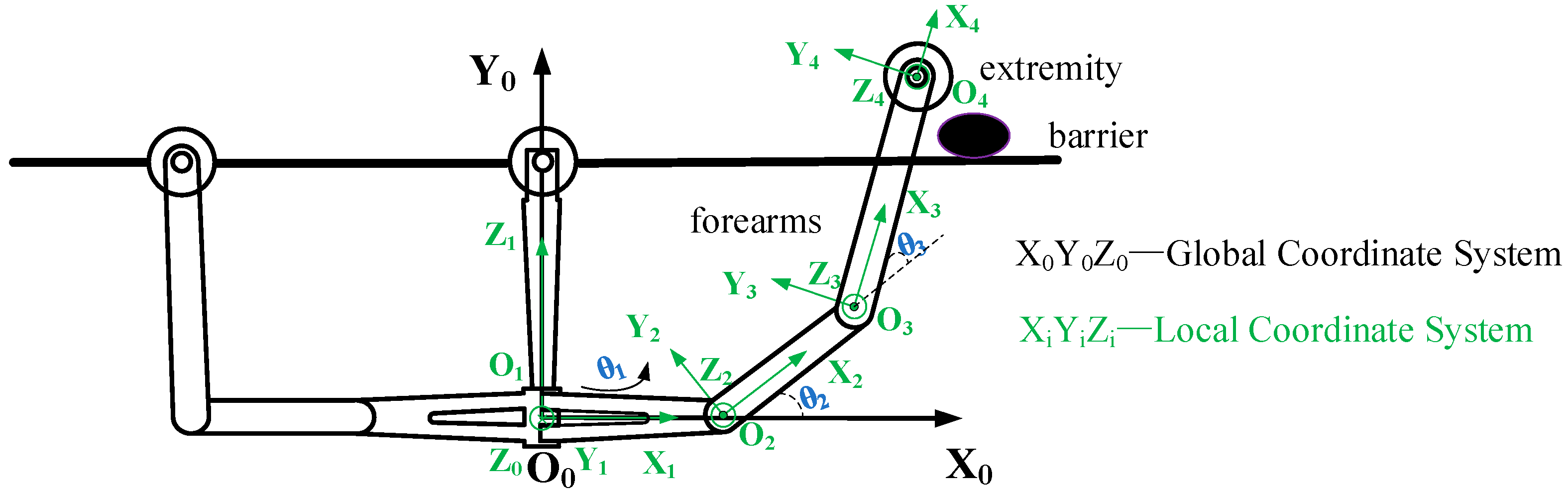
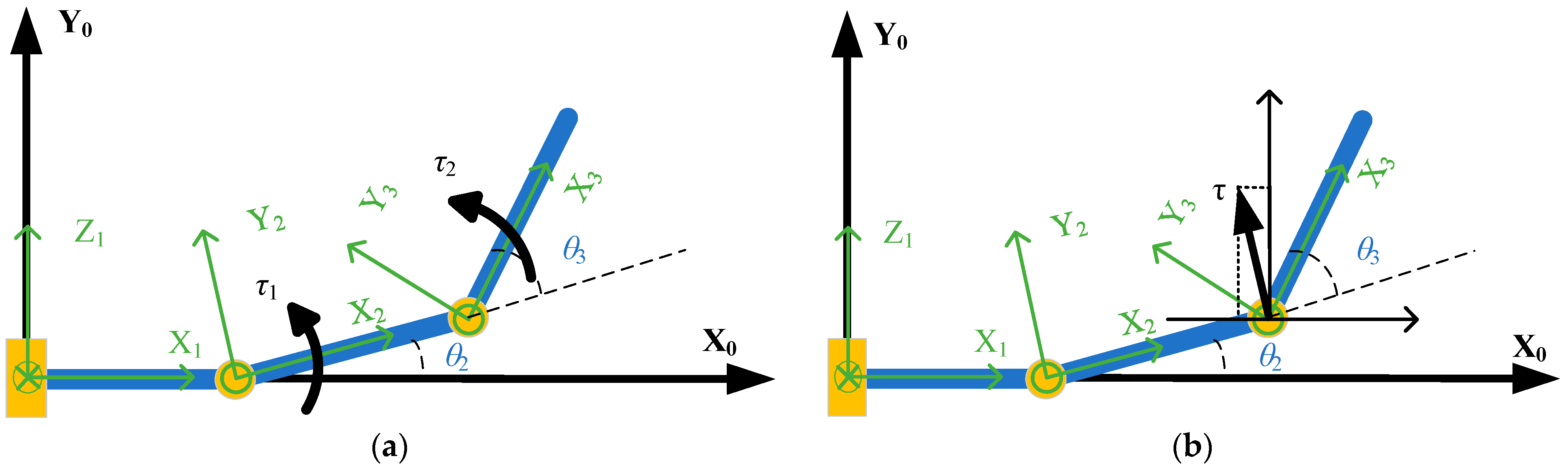
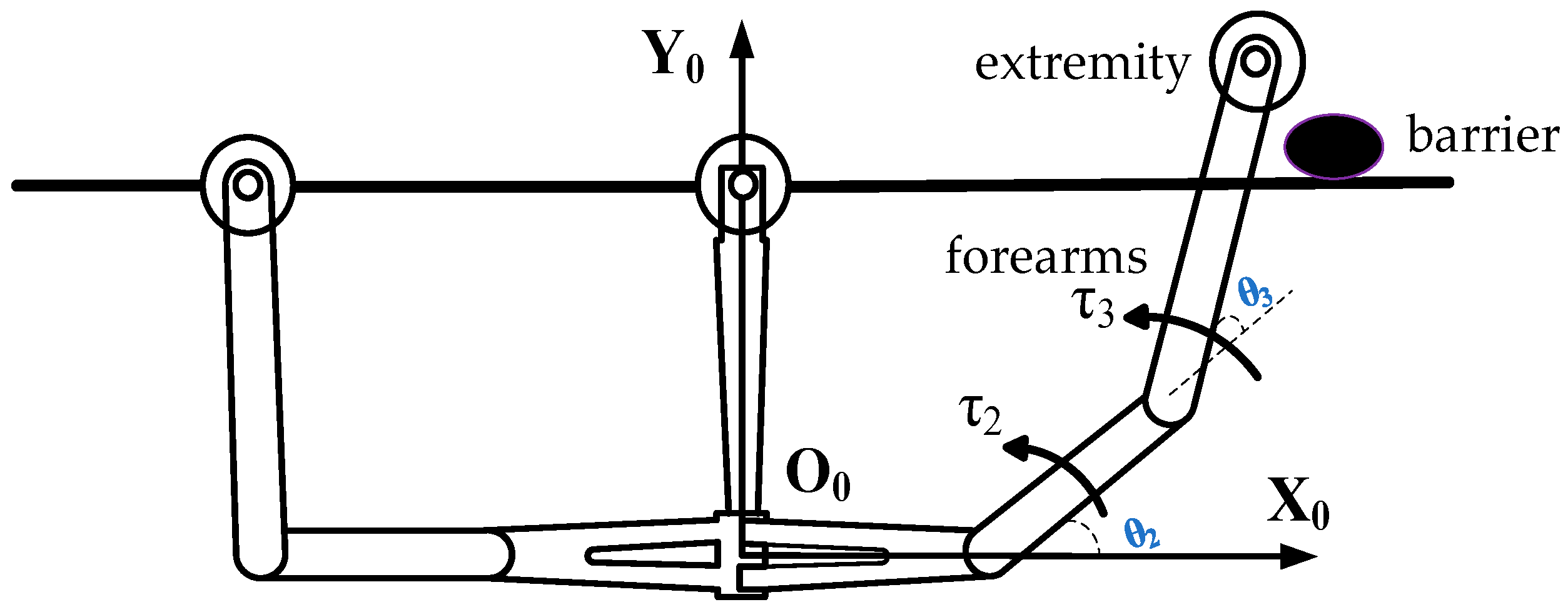
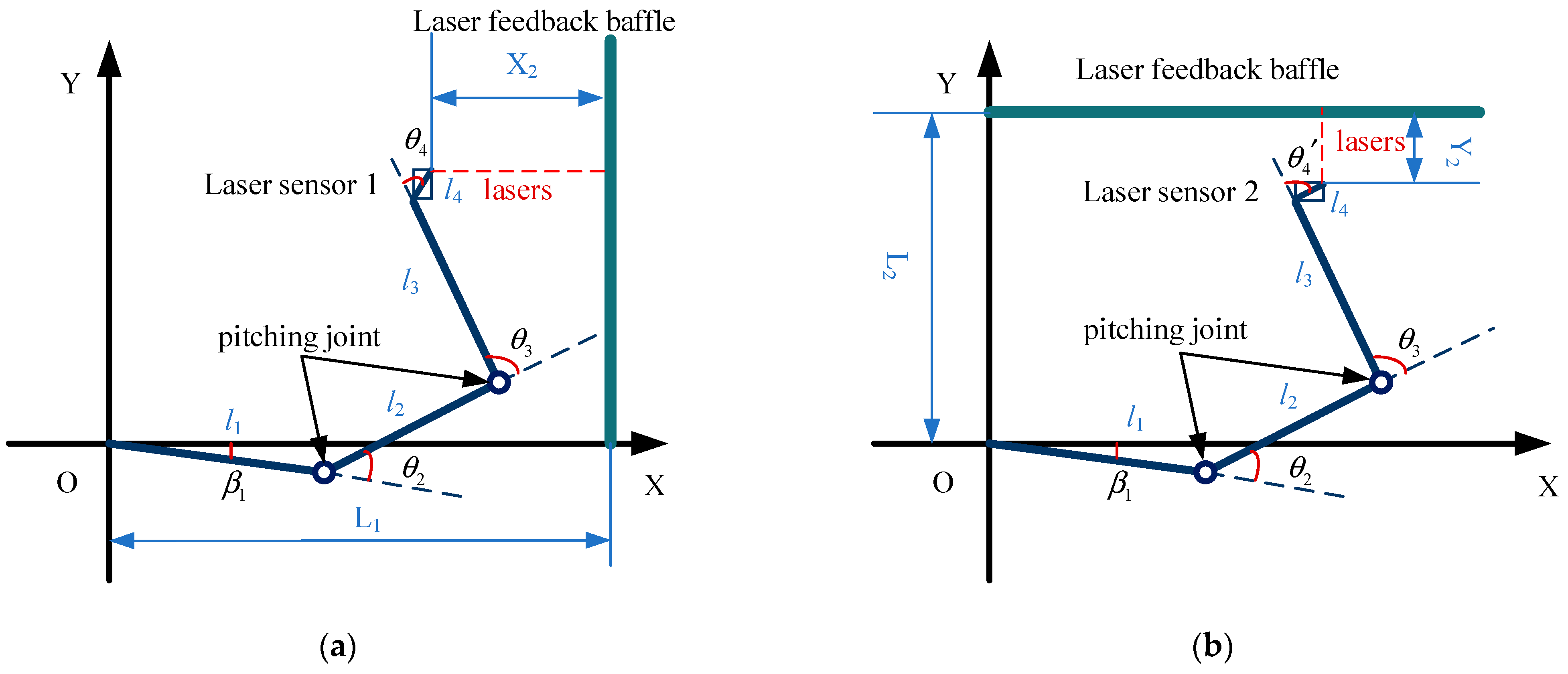
2. Kinematic Analysis

This paper analyzes rigid–flexible coupling dynamics based on a three-armed overhead line mobile robot configuration. Taking the overhead line as the motion environment, for the obstacles on the overhead line, the obstacle-crossing action process [31] is shown in Figure 1. The figure shows the movement of the robot with different robotic arms crossing obstacles on the overhead line. This paper focuses on analyzing one of these obstacle-crossing actions.

For the robot forearm obstacle-crossing action, the D-H coordinate system is established as shown in Figure 2, and the D-H parameter table is shown in

Table 1. D-H parameter sheet.

Connecting Rod i	θi	αi−1	ai−1	di
1	θ1	−90°		0
2	θ2	90°	l1	0
3	θ3	0	l2	0
4		0	l3	0

.

The transformation matrix between adjacent links is as follows:

$${}_1{}^{0}T=\left[\begin{array}{cccc}1& 0& 0& 0\\ 0& 0& 1& 0\\ 0& -1& 0& 0\\ 0& 0& 0& 1\end{array}\right],{}_2{}^{1}T=\left[\begin{array}{cccc}{\mathrm{c}}_1& -{\mathrm{s}}_1& 0& l_1\\ 0& 0& 1& 0\\ {\mathrm{s}}_1& {\mathrm{c}}_1& 0& 0\\ 0& 0& 0& 1\end{array}\right],{}_3{}^{2}T=\left[\begin{array}{cccc}{\mathrm{c}}_2& -{\mathrm{s}}_2& 0& l_2\\ {\mathrm{s}}_2& {\mathrm{c}}_2& 0& 0\\ 0& 0& 1& 0\\ 0& 0& 0& 1\end{array}\right],{}_4{}^{3}T=\left[\begin{array}{cccc}{\mathrm{c}}_3& -{\mathrm{s}}_3& 0& 0\\ {\mathrm{s}}_3& {\mathrm{c}}_3& 0& 0\\ 0& 0& 1& 0\\ 0& 0& 0& 1\end{array}\right]$$

The end position relative to the base coordinate system is as follows:

$${}_4{}^{0}T={}_1{}^{0}T{}_2{}^{1}T{}_3{}^{2}T{}_4{}^{3}T=\left[\begin{array}{cccc}{c}_1\cdot c_{23}-s_1\cdot s_{23}& -c_1\cdot s_{23}-s_1\cdot c_{23}& 0& c_1\cdot \left(l_3\cdot c_2+l_2\right)-s_1\cdot l_3\cdot s_2+l_1\\ s_1\cdot c_{23}-c_1\cdot s_{23}& -s_1\cdot s_{23}-c_1\cdot c_{23}& 0& s_1\cdot \left(l_3\cdot c_2+l_2\right)-c_1\cdot l_3\cdot s_2\\ 0& 0& -1& 0\\ 0& 0& 0& 1\end{array}\right]$$

(1)

where ${}_1{}^{0}T$ is the transformation matrix from link 1 to the base coordinate system of the robot system and ${}_2{}^{1}T,{}_3{}^{2}T,{}_4{}^{3}T$ is the matrix of neighboring linkage transformations. ${\mathrm{c}}_2=\cos {\theta }_2$, ${\mathrm{c}}_3=\cos {\theta }_3$, $s_2=\sin {\theta }_2$, $s_3=\sin {\theta }_3$, ${\mathrm{c}}_{23}=\cos ({\theta }_2+{\theta }_3)$, ${\mathrm{s}}_{23}=\sin ({\theta }_2+{\theta }_3)$.

Under ideal rigidity conditions, the trajectory of the robot forearm lift was planned using the cubic polynomial trajectory Formula (2). The initial angles of the two forearm joints were 0 and π/2, respectively, and the final angles were π/10 and π/6, with a completion time set to 5 s. The curves of the angle, angular velocity, and angular acceleration for the two forearm joints are shown in Figure 3.

$$\left\{\begin{array}{l}{\theta }_2(t)=a_0+a_{1}t+a_2{t}^2+a_3{t}^3\\ {\theta }_3(t)=b_0+b_{1}t+b_2{t}^2+b_3{t}^3\end{array}\right.$$

(2)

3. Rigid–Flexible Coupling Dynamic Analysis

3.1. Rigid Dynamics

In this paper, the rigid–flexible coupling dynamics of the robot forearm lifting over obstacles is analyzed as shown in Figure 4.

The kinetic and potential energies of robot forearm link 2 are, respectively:

$$\left\{\begin{array}{l}{T}_2={\displaystyle \frac{1}{2}}{m}_2{v_2}^2+{\displaystyle \frac{1}{2}}{I}_2{{\omega }_2}^2={\displaystyle \frac{1}{2}}{m}_2{l_2}^2{{\dot{\theta }}_2}^2\\ U_2=m_{2}g{l}_2\sin {\theta }_2\end{array}\right.$$

(3)

The kinetic and potential energies of robot forearm link 3 are, respectively:

$$\left\{\begin{array}{l}{T}_3={\displaystyle \frac{1}{2}}{m}_3{v_3}^2+{\displaystyle \frac{1}{2}}{I}_3{{\omega }_3}^2={\displaystyle \frac{1}{2}}{m}_3{v_3}^2\\ U_3=m_{3}g\left(l_2{s}_2+l_3{s}_{23}\right)\end{array}\right.$$

(4)

where $\sin \left({\theta }_2-{\theta }_3\right)=s_2{c}_3-c_2{s}_3$, $\cos \left({\theta }_2-{\theta }_3\right)=c_2{c}_3+s_2{s}_3$, $\cos \left({\theta }_2+{\theta }_3\right)=c_{23}$, and $\sin \left({\theta }_2+{\theta }_3\right)=s_{23}$.

The kinetic and potential energies of the overhead line mobile robot system are as follows:

$$\left\{\begin{array}{c}T={\displaystyle \frac{1}{2}}{m}_3\left[\left({l_2}^2+2l_2{l}_3{c}_2+{l_3}^2\right){{\dot{\theta }}_2}^2\right]+{\displaystyle \frac{1}{2}}{m}_3\left[\left(2l_2{l}_3{c}_2+2{l_3}^2\right){\dot{\theta }}_2{\dot{\theta }}_3+{l_3}^2{{\dot{\theta }}_3}^2\right]+{\displaystyle \frac{1}{2}}{m}_2{l_2}^2{{\dot{\theta }}_2}^2\\ U=\left(m_2+m_3\right)g{l}_2{s}_2+m_{3}g{l}_3{s}_{23}\end{array}\right.$$

(5)

where m₂ and l₂ are the mass and length of the second robotic arm, respectively, m₃ and l₃ are the mass and length of the third robotic arm, θ₂ is the joint angle of the second arm, θ₃ is the joint angle of the third arm, T represents the kinetic energy of the robot, and U represents the potential energy of the robot.

Disregarding the joint friction loss, using the Lagrangian kinetic equation yields the following:

$${\displaystyle \frac{d}{dt}}{\displaystyle \frac{\partial T}{\partial {\dot{\theta }}_i}}-{\displaystyle \frac{\partial T}{\partial {\theta }_i}}+{\displaystyle \frac{\partial U}{\partial {\theta }_i}}={\tau }_i$$

(6)

where ${\theta }_i$ is the rotation angle of the robotic arm and ${\tau }_i$ is the motor output torque.

The kinetic and potential energies of the robot are obtained by substituting them into the Lagrangian dynamics equations as follows:

$$\left\{\begin{array}{c}{\tau }_2=\left(m_3{l_3}^2+\left(m_2+m_3\right){l_2}^2\right){\ddot{\theta }}_2+m_3{l}_3\left(l_3+3l_2\left(c_2-s_3\right)\right){\ddot{\theta }}_3-2m_3{l}_2{l}_3{s}_3{\dot{\theta }}_2{\dot{\theta }}_3+m_3{l}_{3}g{c}_{23}+\left(m_2+m_3\right)g{l}_2{c}_2\\ {\tau }_3=m_3{l}_2{l}_3{c}_3{\ddot{\theta }}_2+m_3{l}_2{l}_3{s}_3{{\dot{\theta }}_2}^2+m_3{l}_{3}g{c}_{23}+m_3{l_3}^2\left({\ddot{\theta }}_2+{\ddot{\theta }}_3\right)\end{array}\right.$$

(7)

where m₂ = 0.7 kg, m₃ = 0.7 kg, l₂ = 0.2 m, and l₃ = 0.2 m.

In this paper, the dynamics of the rigid–flexible coupled system is established by combining the dynamic characteristics of the overhead line environment and the dynamic characteristics of the rigid robot analytically, so the rigid dynamics of the overhead line are the basis for establishing accurate rigid–flexible coupled dynamics. In order to verify the correctness and reasonableness of the rigid–flexible coupled dynamics model of the overhead line mobile robot established in this paper, the established rigid dynamics model was simulated and verified. Using the planned trajectory shown in Figure 3 as the input, the theoretical joint torque under rigid conditions was calculated using numerical simulation software based on Equation (7). Meanwhile, dynamic simulation software was used to perform motion simulations on the robot model, obtaining the joint torque from the simulation results. The simulation results are shown in Figure 5b,c. The calculated torque matches the torque obtained from the simulation, so the simulation results show that the rigidity dynamics model of the overhead line mobile robot is valid.

3.2. Rigid–Flexible Coupling Dynamics

Rigid–flexible coupled dynamics was used to further investigate the complex dynamical phenomena of rigid and flexible body interaction on the basis of rigid dynamics. The overhead line, as the operating environment of the mobile robot on the line, can be regarded as the flexible base of the robot, so the deformation of the flexible base will affect the end position of the mobile robot on the overhead line. Zhang [32] established a simplified vertical dynamics model of scissor seat suspension and utilized a spring–damping system to describe the vertical dynamics model of scissor seat suspension. Sharifnia [33] presented a model for dynamic and vibration analysis of a robot with a flexible mobile platform and assumed that the in-plane bending stiffness of the beam is much higher than the out-of-plane bending stiffness, thus neglecting the in-plane transverse vibration of the beam. In this study, it is assumed that the overhead line has sufficiently high bending, twisting, and shear stiffness, so its out-of-plane swaying can be neglected [34].

Figure 6 illustrates the schematic of the auxiliary pole model for the overhead line. In engineering fields such as overhead transmission lines, cable structures, and ropeway transport systems, researchers often use spring–damping systems to simulate the dynamic behavior of flexible overhead structures [35]. This simplified model effectively captures the key dynamic characteristics of the overhead line, making analysis and control more feasible. In this study, we simplified the overhead line into a spring–damping system based on its dynamic properties. This approach is particularly effective for small-amplitude vibrations, where the response is mainly governed by elasticity and damping. To simulate the deformation of the flexible line, the model replaces a 2 m section of the overhead line with two auxiliary poles. Additionally, to represent the mechanical properties of the flexible environment, the model incorporates springs and dampers. The springs simulate the longitudinal deformation of the overhead line, while the dampers account for energy dissipation. For simplicity and to focus on key dynamic characteristics, Figure 6 only considers vertical vibrations in the Y direction.

The flexible environment is represented as a spring damper, and the vibrations forced by the robot’s motion on the overhead line are forced vibrations [36]. The overhead line is equivalent to the flexible base of the robot, thus adding a degree of freedom of the base to the rigid dynamics of the robot. A differential equation for the dynamics of the forced vibration of the overhead line is as follows:

$$m_0{\ddot{y}}_0+c{\dot{y}}_0+k{y}_0=f_0$$

(8)

where m₀ is the total weight of the robotic system, c is the virtual damping coefficient, k is the virtual spring coefficient, f₀ is the forcing on the overhead line, and y₀ is the longitudinal vibration displacement of the overhead line.

The general form of the rigid–flexible coupled dynamics of an overhead line mobile robot is as follows:

$$\left[\begin{array}{ccc}{M}_0& 0& 0\\ 0& M_{11}& M_{12}\\ 0& M_{21}& M_{22}\end{array}\right]\left[\begin{array}{c}{\ddot{y}}_0\\ {\ddot{\theta }}_2\\ {\ddot{\theta }}_3\end{array}\right]+\left[\begin{array}{ccc}{C}_0& 0& 0\\ 0& C_{11}& C_{12}\\ 0& C_{21}& C_{22}\end{array}\right]\left[\begin{array}{c}{\dot{y}}_0\\ {\dot{\theta }}_2\\ {\dot{\theta }}_3\end{array}\right]+\left[\begin{array}{c}{G}_0\\ G_2\\ G_3\end{array}\right]=\left[\begin{array}{c}{f}_0\\ {\tau }_2\\ {\tau }_3\end{array}\right]$$

(9)

where $M_0=m_0$, $C_0=\mathrm{c}$, $G_0=k{y}_0$, $M_{11}=I_1+a_1{\mathrm{c}}_2+\left(a_2+2a_3{\mathrm{c}}_2\right){\mathrm{c}}_{23}$, $M_{22}=I_2+a_1+a_2+2a_2{\mathrm{c}}_3$, $M_{12}=M_{21}=M_{13}=M_{31}=0$, $M_{23}=M_{32}=a_2+a_3\cos \left({\theta }_3\right)$, $M_{33}=I_3+a_2$, $C_{12}=C_{21}=-{\displaystyle \frac{1}{2}}{a}_1{\dot{\theta }}_1\sin \left(2{\theta }_2\right)-{\displaystyle \frac{1}{2}}{a}_2{\dot{\theta }}_1\sin \left(2{\theta }_2+2{\theta }_3\right)-a_3{\dot{\theta }}_1\sin \left(2{\theta }_2+{\theta }_3\right)$, $C_{11}=-{\displaystyle \frac{1}{2}}{a}_1{\dot{\theta }}_2\sin \left(2{\theta }_2\right)-{\displaystyle \frac{1}{2}}{a}_2\left({\dot{\theta }}_2+{\dot{\theta }}_3\right)\sin 2\left({\theta }_2+{\theta }_3\right)-a_3{\dot{\theta }}_2\sin \left(2{\theta }_2+{\theta }_3\right)-a_3{\dot{\theta }}_3{\mathrm{c}}_2{\mathrm{s}}_{23}$, $C_{13}=-C_{31}=-{\displaystyle \frac{1}{2}}{a}_1{\dot{\theta }}_1\sin \left(2{\theta }_2+2{\theta }_3\right)-a_3{\dot{\theta }}_1{\mathrm{c}}_2{\mathrm{s}}_{23}$, $C_{22}=-a_3{\dot{\theta }}_3{\mathrm{s}}_3$, $C_{23}=-a_3\left({\dot{\theta }}_2+{\dot{\theta }}_3\right){\mathrm{s}}_3$, $C_{32}=-a_3{\dot{\theta }}_2{\mathrm{s}}_3$, $C_{33}=0$, $G_1=0$, $G_2=b_1{\mathrm{c}}_2+b_2{\mathrm{c}}_{23}$, $G_3=b_2{\mathrm{c}}_{23}$, $a_1=m_2{r_2}^2+m_3{l_2}^2$, $a_2=m_3{r_3}^2$, $a_3=m_3{r}_3{l}_2$, $b_1=\left(m_2{r}_2+m_3{l}_2\right)g$, $b_2=m_3{r}_{3}g$.

In this paper, a rigid robot coupled with a flexible overhead line was simplified to a spring–damped system when analyzing the obstacle-crossing action. This reduced the degrees of freedom of the system, thereby streamlining the computation process. Although the model has been simplified, it does not omit the primary characteristic of vibration—y. This simplification method effectively retains the vibration characteristics of the overhead line, ensuring that the system’s dynamic behavior is accurately reflected while improving computational efficiency. This method significantly reduces the computational load and improves overall computational efficiency. It provides an effective model basis for the analysis and control of the rigid–flexible coupled dynamics of the subsequent overhead line mobile robot.

For the action of the forearm carrying the front line, the vertical force applied to the overhead line due to the movement of the robotic arm is analyzed. Figure 7 shows the force analysis diagram, which primarily illustrates the force generated by the robotic arm’s movement and its effect on the vertical direction of the overhead line. Since the robot forearm is in an elevated state, the forearm’s end does not collide with the overhead line, and therefore, the force acting on the overhead line is the difference between the robot’s total weight and the joint torque force in the vertical direction of the mechanical arm. Based on Newton’s third law, the relationship between the forced force on the overhead line and the robot’s trajectory is established as follows:

$$\begin{array}{c}{f}_0={\tau }_2\cos {\theta }_2+{\tau }_3\cos \left({\theta }_2+{\theta }_3\right)-m_{0}g\\ \hspace{1em}=[m_3{l_3}^2\left({\ddot{\theta }}_2+{\ddot{\theta }}_3\right)+m_3{l}_2{l}_3{c}_2\left(2{\ddot{\theta }}_2+{\ddot{\theta }}_3\right)+\left(m_2+m_3\right){l_2}^2{\ddot{\theta }}_2-m_3{l}_2{l}_3{s}_3{\ddot{\theta }}_3\\ \hspace{1em}\hspace{1em}-2m_3{l}_2{l}_3{s}_3{\dot{\theta }}_2{\dot{\theta }}_3+m_3{l}_{3}g{c}_{23}+\left(m_2+m_3\right)g{l}_2{c}_2]c_2+[m_3{l}_2{l}_3{c}_3{\ddot{\theta }}_2+m_3{l}_2{l}_3{s}_3{{\dot{\theta }}_2}^2\\ \hspace{1em}\hspace{1em}+m_3{l}_{3}g{c}_{23}+m_3{l_3}^2\left({\ddot{\theta }}_2+{\ddot{\theta }}_3\right)]c_{23}-m_{0}g\end{array}$$

(10)

where m₀ is the total robot mass.

From Equation (10), it can be seen that as the robot forearm joint angles θ₂ and θ₃ change, the forced force f₀ acting on the overhead line also changes. This indicates that the motion of the robot joints not only affects its own dynamic behavior but also causes fluctuations in the force applied to the overhead line, which in turn influences the mechanical response of the entire system. Therefore, there exists a close coupling relationship between the changes in the robot joint angles and the forced force on the overhead line.

The force analysis diagram of the overhead line mobile robot system is shown in Figure 8. The vibration equation of the overhead line is derived from the rigid–flexible coupling dynamics equation as follows:

$$M_0{\ddot{y}}_0+C_0{\dot{y}}_0+G_0=f_0$$

(11)

From Equation (11), it can be seen that the robot joint angle affects the forcing force on the overhead line, which causes the line to vibrate. The vibration of the overhead line then impacts the movement of the robot joints, creating a coupling relationship.

Since directly solving the equation is difficult when facing complex external excitations, we used the impulse response and convolution integral method. Using the convolution integral method [37], we treated any excitation as a series of pulses, which eliminated the need to solve the differential equation each time the input is changed.

At any moment $t=s$, the corresponding time increment is $\Delta s$. The force corresponds to a pulse of size $F(s)\Delta s$. By summing, the total response caused by each pulse in the sequence can be calculated as:

$$y(t)\approx {\displaystyle \sum F(s)\delta (t-s)\Delta s}$$

(12)

Let $\Delta s\to 0$ and take the limit; Equation (10) can then be expressed in integral form as:

$$y(t)={\displaystyle {\int }_0^{t}F(s)\delta (t-s)\mathrm{ds}}$$

(13)

Substituting $\delta (t-s)=e^{-\zeta {\omega }_n(t-s)}\sin {\omega }_d\left(t-s\right)$ gives the system response:

$$y(t)={\displaystyle \frac{1}{m{\omega }_d}}{\displaystyle {\int }_0^{t}F(s)e^{-\zeta {\omega }_n(t-s)}\sin {\omega }_d\left(t-s\right)\mathrm{ds}}$$

(14)

When $t=0$, under the action of any excitation $F(t)$, the system’s initial displacement and initial velocity are $x\left(0\right)=x_0$ and $\dot{x}\left(0\right)={\dot{x}}_0$.

The system’s response is the sum of the responses caused by the excitation and initial conditions. The response of a single-degree-of-freedom damped–spring mass system to any initial conditions and excitation is:

$$y_0(t)=e^{-\zeta {\omega }_{n}t}\left(y_0\cos {\omega }_{d}t+{\displaystyle \frac{{\dot{y}}_0+\zeta {\omega }_n{y}_0}{{\omega }_d}}\sin {\omega }_{d}t\right)+{\displaystyle \frac{1}{m{\omega }_d}}{\displaystyle {\int }_0^{t}f(s)e^{-\zeta {\omega }_n(t-s)}\sin {\omega }_d(t-s)\mathrm{d}s}$$

(15)

where y₀ is the dynamic response, $\zeta$ is the damping ratio, $\zeta =c/c_c$; $c_c$ is the critical damping coefficient, $c_c=2m{\omega }_n$; ${\omega }_n$ is the intrinsic frequency of the vibration coefficients in the absence of damping, ${\omega }_n=\sqrt{k/m}$; ${\omega }_d$ is the damped free vibration circular frequency, ${\omega }_d=\sqrt{1-{\zeta }^2}{\omega }_n$; and s is the integral variable.

The forced vibration response Equation (15) was used as the basis for the theoretical analysis of reducing the vibration of the overhead line. The equation contains a change in the robot joint trajectory, which is a simplified analysis of the forcing force on the overhead line. Therefore, it is possible to reduce the value of the forcing force by changing the robot joint trajectory to reduce the vibration of the overhead line.

4. Active Compensation Trajectory Analysis

4.1. Under the Conditions of a 2 m Overhead Line

Due to the flexible characteristics of the overhead line and the robot’s gravity, the line sags, causing the robot’s end effector to fall short of the desired height. Therefore, dynamic simulations were conducted based on the obstacle-crossing joint trajectories planned in Section 2. A model of the overhead line mobile robot was built in the dynamics simulation software. Simulations were carried out under both the rigid and flexible conditions of the overhead line. Figure 9 shows the motion trajectories of the robot’s end effector in both the rigid and flexible environments.

The simulation results show that, for the same joint trajectory, the robot’s end in the flexible environment is lower than the end in the ideal state. As the motion of the robot exerts a forcing force on the overhead line, this leads to the vibration of the overhead line. The vibration is transferred to the robot and is reflected in the end vibration of the robot. Due to the damping of the overhead line, the vibration decreases and the trajectory gradually stabilizes. This vibration not only hinders the robot’s normal movement but may also lead to collisions with obstacles [38].

To facilitate control and compensation, this study proposes a simple and effective method to address the following two issues: (1) due to the flexible characteristics of the overhead line, the robot cannot reach the desired trajectory under rigid conditions; and (2) different joint motion trajectories generate different forcing forces on the overhead line, leading to varying vibration peaks in the line’s response. The smaller the vibration peak, the smaller the overhead line’s vibration, and the less impact the overhead line has on the robot. Unlike B-spline trajectory methods, our approach utilizes an active compensation strategy to directly calculate the positions of key trajectory points. It employs constant velocity and segmented constant velocity motion, making the trajectory easier to control while reducing computational load and improving practicality. By adjusting two sets of joint trajectories based on inverse kinematics, the trajectory is brought closer to the desired path. The two adjustment strategies are as follows: (1) The first set of adjustment strategies is to calculate the compensated end position, and the two joints move to the end point at a uniform speed.

The end position of the robot’s forearm in the rigid condition can be calculated as follows:

$$\left\{\begin{array}{l}x=l_2\cos {\theta }_2+l_3\cos \left({\theta }_2+{\theta }_3\right)\\ y=l_2\sin {\theta }_2+l_3\sin \left({\theta }_2+{\theta }_3\right)\end{array}\right.$$

(16)

where x is the horizontal position of the robotic arm’s end effector, and y is the vertical position.

When the robot is in static equilibrium on the overhead line, the maximum displacement produced by the overhead line is assumed to be ΔH_max. Based on the geometric relationship in Figure 6, the displacement produced by the simplified line compared to the rigid line is:

$$\Delta H=-\tan \alpha z+\Delta H_{\max }$$

(17)

where $\tan \alpha ={\displaystyle \frac{\Delta H_{\max }}{L}}$.

From Figure 9, the deviation produced by the forearm end y and the ideal end trajectory of the overhead line mobile robot in the flexible environment can be determined. $\Delta H$ was added to the original planned end trajectory y, keeping x constant, as follows:

$$\left\{\begin{array}{l}x=l_2\cos {{\theta }_2}^{\prime }+l_3\cos \left({{\theta }_2}^{\prime }+{{\theta }_3}^{\prime }\right)\\ y+\Delta H=l_2\sin {{\theta }_2}^{\prime }+l_3\sin \left({{\theta }_2}^{\prime }+{{\theta }_3}^{\prime }\right)\end{array}\right.$$

(18)

Inverse kinematics to actively compensate the robot end at the end of the obstacle-crossing motion. The robotic arm joints 2 and 3 run at a uniform speed to the end point of the obstacle-crossing motion. The uniform velocity time interval is [0, 5] and the trajectory profile is a primary polynomial. The expressions for position, velocity, and acceleration are as follows:

$$\left\{\begin{array}{l}{{\theta }_2}^{\prime }(t)=a_0+a_{1}t\\ {{\dot{\theta }}_2}^{\prime }(t)=a_0\\ {{\ddot{\theta }}_2}^{\prime }(t)=0\end{array}\right.\left\{\begin{array}{l}{{\theta }_3}^{\prime }(t)=b_0+b_{1}t\\ {{\dot{\theta }}_3}^{\prime }(t)=b_0\\ {{\ddot{\theta }}_3}^{\prime }(t)=0\end{array}\right.$$

(19)

where a₀ represents the initial position of the robotic arm, a₁ represents the constant velocity of the second robotic arm during uniform motion, b₀ represents the initial position of the robotic arm, b₁ represents the constant velocity of the second robotic arm during uniform motion.

(2) The second set of adjustment strategies is to consider the position node of the original end trajectory y, the segmented uniform speed running to the node, and the end point of crossing the obstacle.

As shown in Figure 10, the trajectory of the end of the robot forearm gradually levels off after 4.3 s, with a slope of less than 0.1. As such, 4.3 s was chosen as the node for two segments of uniform velocity movement. The first segment runs from the starting point to the node position, and the uniform velocity time interval is [0, 4.3]. The second segment runs from the node position to the end point of the barrier crossing, and the uniform velocity time interval is [4.3, 5].

The joint motion trajectory obtained from the first adjustment strategy is shown in Figure 11a, while the joint motion trajectory obtained from the second adjustment strategy is shown in Figure 11b.

This vibration is caused by the robot’s movements. Based on the system dynamics theory and forced vibration response analysis, the potential vibration situation of the robot under different trajectories was analyzed. Suitable adjusted trajectories were selected to minimize the vibration effects and improve the robot’s operation accuracy and stability. The two sets of adjusted trajectories were substituted into the forcing force f₀ (Equation (10)) to obtain the effects of the two sets of adjusted trajectories on the forced vibration of the robot. The results are shown in Figure 12. The forcing force generated by the second set of adjustment trajectories is significantly smaller than that of the first joint adjustment trajectories. The smaller the forcing force applied to the overhead line, the smaller the vibration generated by the overhead line.

Adjustments were made to the motion trajectories of joints 2 and 3 using the active compensation method mentioned earlier. The system outputs for two different trajectories were calculated to validate the dynamic system response. The system response generated by the trajectories was calculated using the convolution integral (Equation (15)) to analyze and evaluate the dynamic performance of the different trajectory scenarios. Figure 13 was obtained by computing the dynamic response using Equation (15) and extracting its peak value. Figure 14 was derived by substituting the adjusted trajectory sets into Equation (16) and performing the corresponding calculations. The simulation analysis results show that when both sets of end trajectories can reach the desired trajectories, the vibration of the tuned trajectory 2 is relatively smaller and more quickly stabilized, which can effectively reduce the vibration of the system and improve the stability of the robot operation.

4.2. Under the Conditions of a 10 m Overhead Line

Furthermore, to study the impact of the overhead line span on the robot’s end trajectory, we increased the span to 10 m. We performed a simulation analysis on the same joint motion trajectory. The simulation results are shown in Figure 15. The results indicate that, similar to the 2 m overhead line, the overall position of the end effector in the flexible environment is lower than the ideal state, and it also experiences vibrations that gradually stabilize. However, with the increase in overhead line span, both the vibration amplitude and the position error of the end effector increased somewhat.

As shown in Figure 16, the trajectory of the robot’s forearm end gradually becomes more horizontal after 3.5 s, with a slope of less than 0.1. The time of 4.3 s is selected as the node for the two segments of uniform motion. The first segment runs from the starting point to the node position, with a uniform motion time interval of [0, 3.5]. The second segment runs from the node position to the obstacle crossing end point, with a uniform motion time interval of [3.5, 5].

For the overhead line span of 10 m, the same two sets of trajectory adjustment strategies were used for compensation, as shown in Figure 17. The forced forces generated by the two trajectories are depicted in Figure 18. The second set of adjustment strategies also outperformed the first set in reducing vibrations. Moreover, compared to the simulation results under the condition of a 2 m overhead line, the compensated end trajectory requires a greater adjustment to achieve the desired trajectory.

During the uniform walking process, the force exerted by the robot on the overhead line causes the line to undergo sag deformation. To describe this process more accurately, we simplified the overhead line mobile robot system into a flexible overhead line model subjected to a moving concentrated load, as shown in Figure 19. In this paper, the deformation is much smaller than the geometric dimensions of the overhead line. Under the small deformation assumption, the stiffness of the structure is primarily determined by the material’s bending stiffness, and the influence of geometric stiffness can be neglected [39].

Through this model, we can obtain the deflection function of the overhead line as follows:

$$y(x,v,t)=({\displaystyle \frac{R_0}{6}}{x}^3-{\displaystyle \frac{P_0}{6}}{(x-vt)}^3+C_{1}x+C_2)/\mathrm{EI}$$

(20)

where $R_0={\displaystyle \frac{P_0}{L}}\left(L-vt\right),C_1={\displaystyle \frac{P_0}{6L}}\left[(L-vt)(1-L^2)+{(vt)}^3\right],C_2=-{\displaystyle \frac{P_0{(vt)}^3}{6}}$.

Here, y(x, v, t) is the deformation at position x, varying with time t and load velocity v. R₀ and P₀ represent the self-weight of the line and the concentrated force caused by the moving load, respectively. EI is the bending stiffness of the overhead line, where E is the elastic modulus and I is the moment of inertia of the cross-section. C₁ and C₂ are integration constants determined by the boundary conditions. x is the current analysis position, and vt denotes the current position to which the load has moved.

The deformation of the overhead line caused by the mobile robot at different positions is obtained through numerical simulation, as shown in Figure 20.

By compensating for the sag at rest into the rigid trajectory, we obtained the desired end trajectory. By comparing the desired trajectory with the end trajectories obtained from Adjustment Trajectory 1 and Adjustment Trajectory 2, we analyzed the results under a 10 m overhead line span. The simulation results are shown in Figure 21. In the flexible environment, the robot’s end position is still lower than the ideal state and experiences noticeable vibrations. Compared to the 2 m overhead line, the vibration amplitude is greater with the 10 m line. After applying two sets of adjustment strategies for compensation, the second adjustment strategy still performed better than the first. Adjustment Trajectory 2 is closer to the desired trajectory.

5. Experiments

5.1. Experimental Preparations

A simulated two-meter overhead line was constructed in conjunction with the simulation environment data. Based on the forearm crossing action, the established rigid–flexible coupling dynamics model and the validity of the model application method were verified.

The constructed experimental prototype is shown in Figure 22. The overall external dimensions of the overhead line mobile robot prototype were 930 × 260 × 120 mm, and the total weight of the mechanical system was 6.6 kg. The end of the robot’s forearm was equipped with two laser displacement sensors and a WIFI gyroscope angle sensor. The two laser displacement sensors were oriented towards the horizontal X-direction and vertical Y-direction, respectively. A laser feedback baffle was built in these two directions to measure the change in the end of the overhead line mobile robot during the movement.

5.2. Overhead Line Characteristic Parameter Extraction Experiment

The parameters of the segmented spring–damping model in the rigid–flexible coupled dynamical system needed to be measured by the free vibration experiment of the overhead line. Considering the different tension forces of the overhead line before and after loading, the spring–damping coefficient of the virtual passive joint was set as a segmental constant, making the dynamics model closer to the actual environment. The specific steps were as follows:

(1)

Build a two-meter overhead-line experiment platform.

(2)

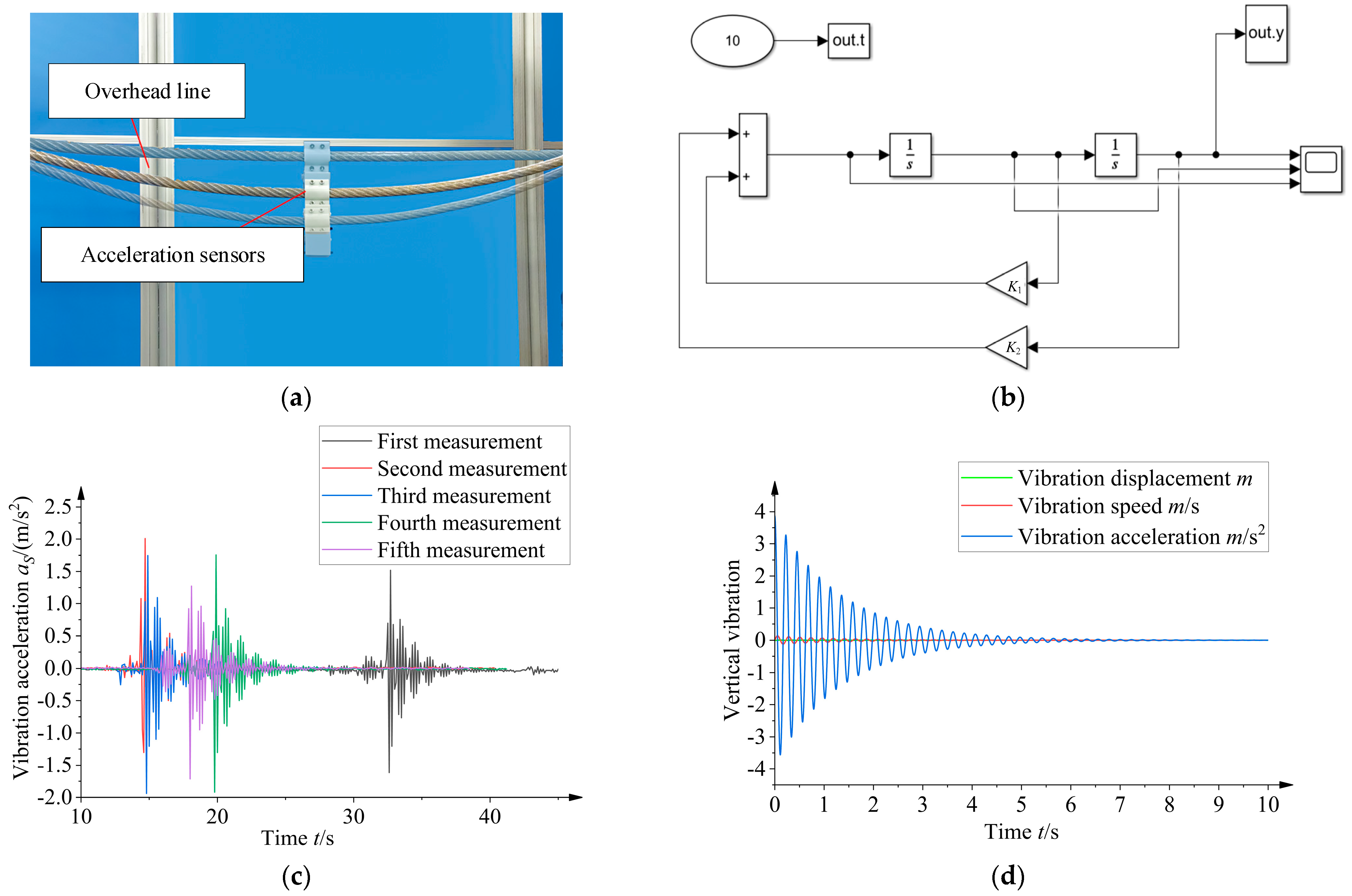
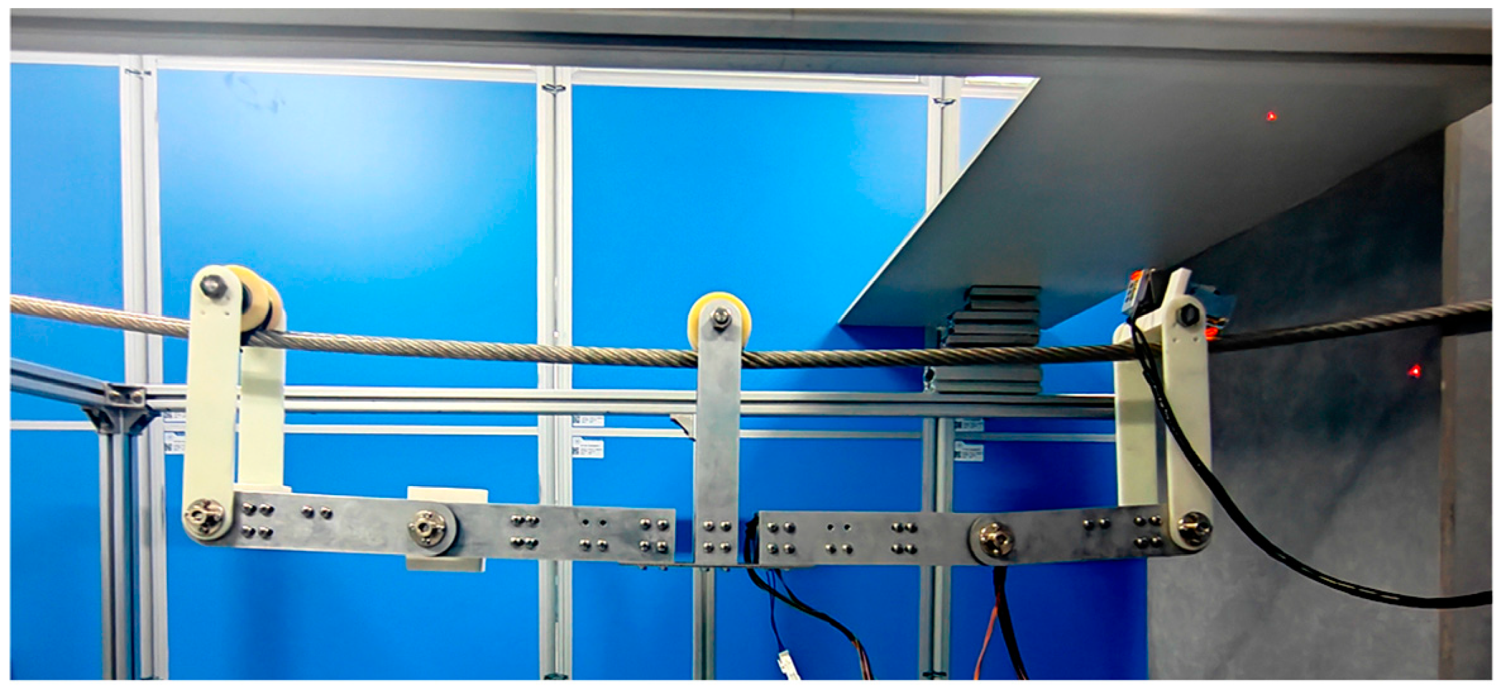
In the middle of the overhead line, install a six-axis gyroscope angle sensor with its Z-axis perpendicular to the ground, as shown in Figure 23a. Measure the distance between the center of the overhead line and the ground, which was 104 mm.

(3)

Suspend a weight, with an equal weight to the robot, from the overhead line. After stabilization, the center of the overhead line drops under its gravity by 0.09 m. Therefore, the initial position of the system was set to 0.09 m and the initial velocity was 0 in the simulation model.

(4)

Remove the weight applied to the overhead line and allow the line to vibrate freely. Record the sensor data and output.

(5)

Repeat the above experimental steps several times. Export the experimental data and process them to obtain the vibration curve of the overhead line.

(6)

Establish a free vibration simulation system in the numerical simulation platform, as shown in Figure 23b.

(7)

Modify the gain module parameter K₁ in the simulation system until the acceleration curve in the oscilloscope is consistent with the vibration acceleration curve measured by the experiment. The assumed spring coefficient and damping coefficient can be obtained. The calculation relationship is as follows:

$$K_1=-{\displaystyle \frac{c}{M}},K_2=-{\displaystyle \frac{k}{M}}$$

(21)

where M is the weight of the initial position of the overhead line, K₁ and K₂ are the system gain parameters, c is the virtual damping coefficient, and k is the virtual spring coefficient.

Five experiments were performed based on the same setup. The free vibration simulation of the spring–damping system yielded the same acceleration vibration curve, as shown in Figure 23c,d. The virtual spring damping parameters of the flexible system under heavy load were obtained: the spring coefficient of the system is 6468 N/m, the damping coefficient is 12.54 kg/s, and the vibration circular frequency ω is 31.4 rad/s.

To further analyze the impact of these parameters on the system’s behavior, this paper examines the effects of the damping coefficient c and spring constant k on the system’s vibration response. With a fixed spring constant k = 6468 N/m and a virtual damping coefficient c = 12.54 N·s/m, the virtual damping coefficient c and spring constant k are varied. Figure 24 shows the system’s vibration response under different virtual damping and spring constants. As shown in Figure 24a, with an increase in the damping coefficient, the system’s vibration amplitude gradually decreases, and the vibration frequency also decreases. As shown in Figure 24b, the increase in the spring constant results in a higher vibration frequency, but the change in vibration amplitude is minimal.

5.3. Experiment and Analysis of Actively Compensated Trajectory Motion

To verify the effectiveness of using the rigid–flexible coupling dynamic model for output response to determine and select an active compensation trajectory method, an experimental validation of the robot’s active compensation trajectory was conducted in an overhead line environment with a span of two meters. The initial state of the overhead line mobile robot is shown in Figure 25, and the experimental process is shown in Figure 26. The specific experimental steps were as follows:

(1)

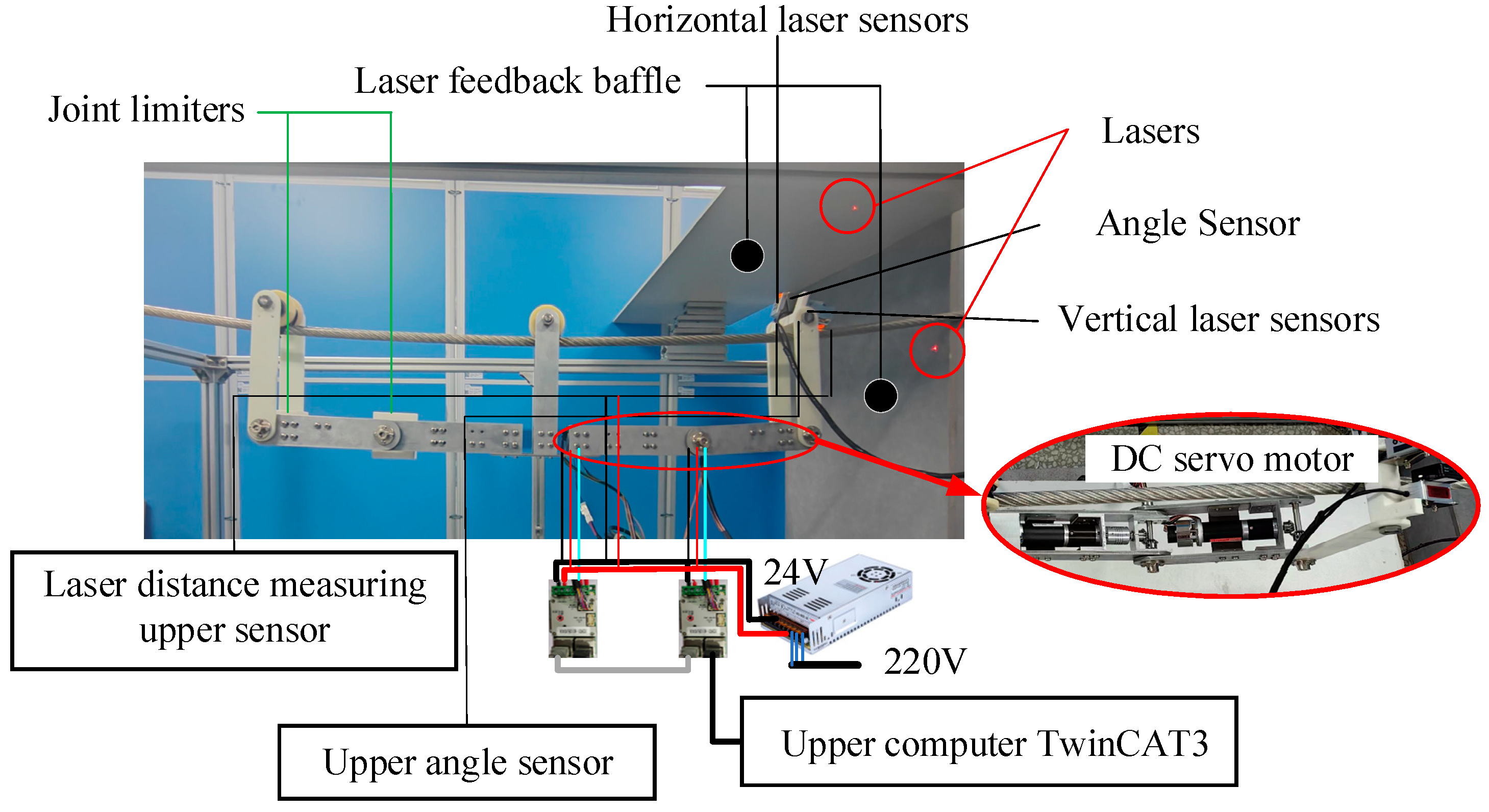
Power on the laser displacement sensor and the angle sensor, and connect them to their corresponding host computers. The sensor parameters are shown in

Table 2. Sensor data.

Sensor Model	Range	Accuracy	Output Format	Main Function	Manufacturer, City, and Country
Laser Sensor BL-200NZ-485	±80 mm	0.2 mm	RS485output	Measure the precise distance of objects	JORMU, Shenzhen, China.
Laser Sensor BL-400NZ-485	±200 mm	0.8 mm	RS485output	Measure the precise distance of objects	JORMU, Shenzhen, China.
Angle Sensor WT901WIFI	X, Z: ±180°; Y: ±90°	XY: 0.2°; Z: 1°	Digital Signal	Detect deflection angle	WIT Intelligent, Huizhou, China.

.

(2)

Power on the motors. Using the host computer, adjust manipulator 2 to form a 40° angle with the horizontal direction. Adjust manipulator 3 to be perpendicular to manipulator 2.

(3)

Adjust the laser displacement sensor at the starting point position to be parallel to the laser feedback baffle, ensuring that the laser at the initial position vertically illuminates the baffle. Align the Z-axis of the angle sensor perpendicular to the ground, and zero out all three sensors.

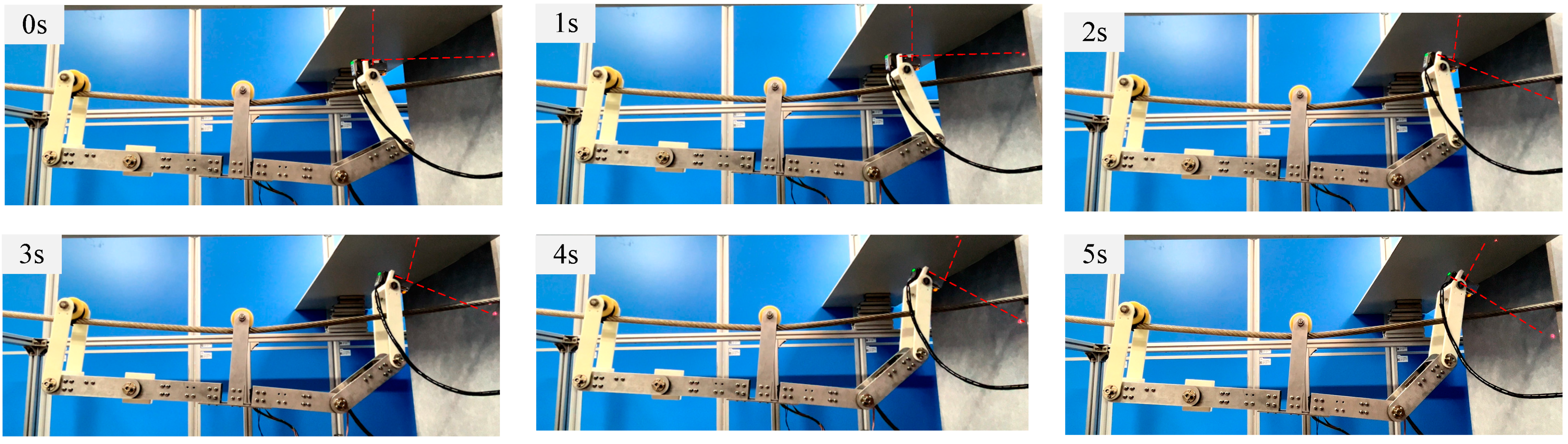
(4)

Conduct multiple experiments on each trajectory adjustment, collect sensor data, and perform data processing.

Process the collected end effector data according to the relationships shown in Figure 27. The relationships are as follows:

$$\left\{\begin{array}{l}{X}_2=L_1-\left[l_1\cos {\beta }_1+l_2\cos \left({\beta }_1+{\theta }_2\right)+l_3\cos \left({\beta }_1+{\theta }_2+{\theta }_3\right)+l_4\cos \left({\beta }_1+{\theta }_2+{\theta }_3+{\theta }_4\right)\right]\\ Y_2=L_2-\left[l_1\sin {\beta }_1+l_2\sin \left({\beta }_1+{\theta }_2\right)+l_3\sin \left({\beta }_1+{\theta }_2+{\theta }_3\right)+l_4\sin \left({\beta }_1+{\theta }_2+{\theta }_3+{{\theta }_4}^{\prime }\right)\right]\end{array}\right.$$

(22)

where X₂ represents the distance from the end of the robot’s forearm to laser barrier 1, Y₂ represents the distance from the end of the robot’s forearm to laser barrier 2, L₁ represents the distance from laser feedback barrier 1 to the robot’s mid-arm coordinate axis Y, and L₂ represents the distance from laser feedback barrier 2 to the robot’s mid-arm coordinate axis X.

Here, β₁ is the pitch angle of the robot’s forearm manipulator due to changes in the robot’s center of gravity during the experimental process, measured as β₁ ≠ 0; θ₂ and θ₃ are the pitch joint angles; and θ₄ and θ₄′ are the deflection angles of laser sensors 1 and 2, respectively.

After data processing, the trajectory data were compared and analyzed, as shown in Figure 28. Trajectory adjustment 1 is the end-effector trajectory of the robotic arm obtained based on the first set of adjustment strategies. Trajectory adjustment 2 is the end-effector trajectory of the robotic arm obtained based on the second set of adjustment strategies. The experimental results show that compared with the original trajectories, the two sets of optimized trajectories are closer to the desired trajectories in the Y direction. The errors are shown in

Table 3. Trajectory error table.

Trajectory	Maximum Error (mm)	Average Error (mm)	Root Mean Square Error (mm)	Amount of Change in Trajectory Velocity (mm/s)
Original trajectory	30.12	24.28	24.46	82.60
Trajectory adjustment 1 of the experiment	36.87	13.25	15.51	216.72
Trajectory adjustment 2 of the experiment	21.77	11.55	13.10	124.61

; trajectory adjustment 1 reduces the average error by 1.83 times compared to the original trajectory, and trajectory adjustment 2 reduces the average error by 2.1 times compared to the original trajectory.

Reference [40] uses an error compensation method based on modifying the initial planned trajectory. In contrast, the compensation strategy proposed in this study is based on a uniform adjustment of the trajectory, which better adapts to dynamic changes in the flexible structure. This allows for smoother trajectory adjustments and reduces the impact of the flexible overhead line. The average trajectory error in this study was reduced by 52.43% compared to the uncompensated case, which is a 1.04% improvement over the 51.39% reduction reported in [40]. This result demonstrates that the proposed method offers superior vibration suppression and trajectory control in flexible environments, significantly enhancing the stability and accuracy of the robot system.

There is a certain deviation between the simulation results and the experimental results, as shown in Figure 29. The theoretical and experimental trajectory errors are shown in

Table 4. Theoretical and experimental trajectory error table.

Trajectory	Maximum Error (mm)	Average Error (mm)	Root Mean Square Error (mm)
Trajectory adjustment 1	39.46118	14.45028375	3.801352884
Trajectory adjustment 2	39.00831	14.06134542	3.749846053

. These deviations primarily arise from the following factors: sensor measurement errors, robot execution errors, uncertainties in the flexible environment, and the simplified assumptions in the dynamic model. These factors collectively lead to an imperfect match between the actual system behavior and the simulation model. However, the experimental results show that the execution performance of the second set of adjusted trajectories is closer to the simulation trajectory compared to the first set, indicating that the second set of compensation strategies is more applicable in real-world environments.

6. Conclusions

In this paper, a rigid–flexible coupled dynamic model is established based on the substructure method and the Lagrange method. By comparing the impact of the trajectory before and after adjustment on the end operation of the overhead line mobile robot, the following conclusions are drawn:

(1)

Based on the Lagrange method and the substructure method, this study constructs a rigid–flexible coupled dynamic model of the mobile robot that considers the longitudinal deformation and vibration of the overhead line. The proposed model provides a more detailed description of the dynamic coupling between the robot and the flexible line. This study offers a new perspective for the academic community in this field of research.

(2)

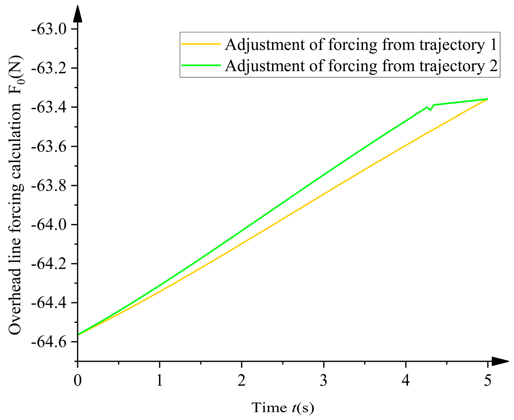
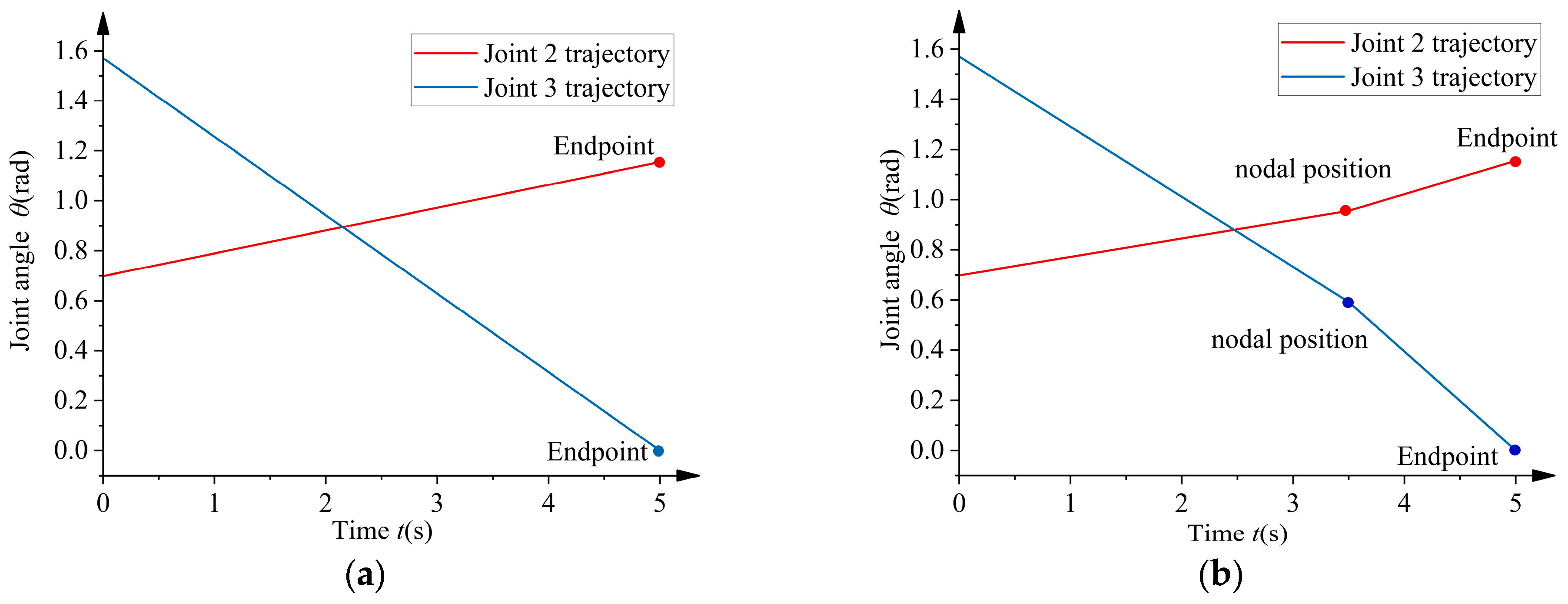
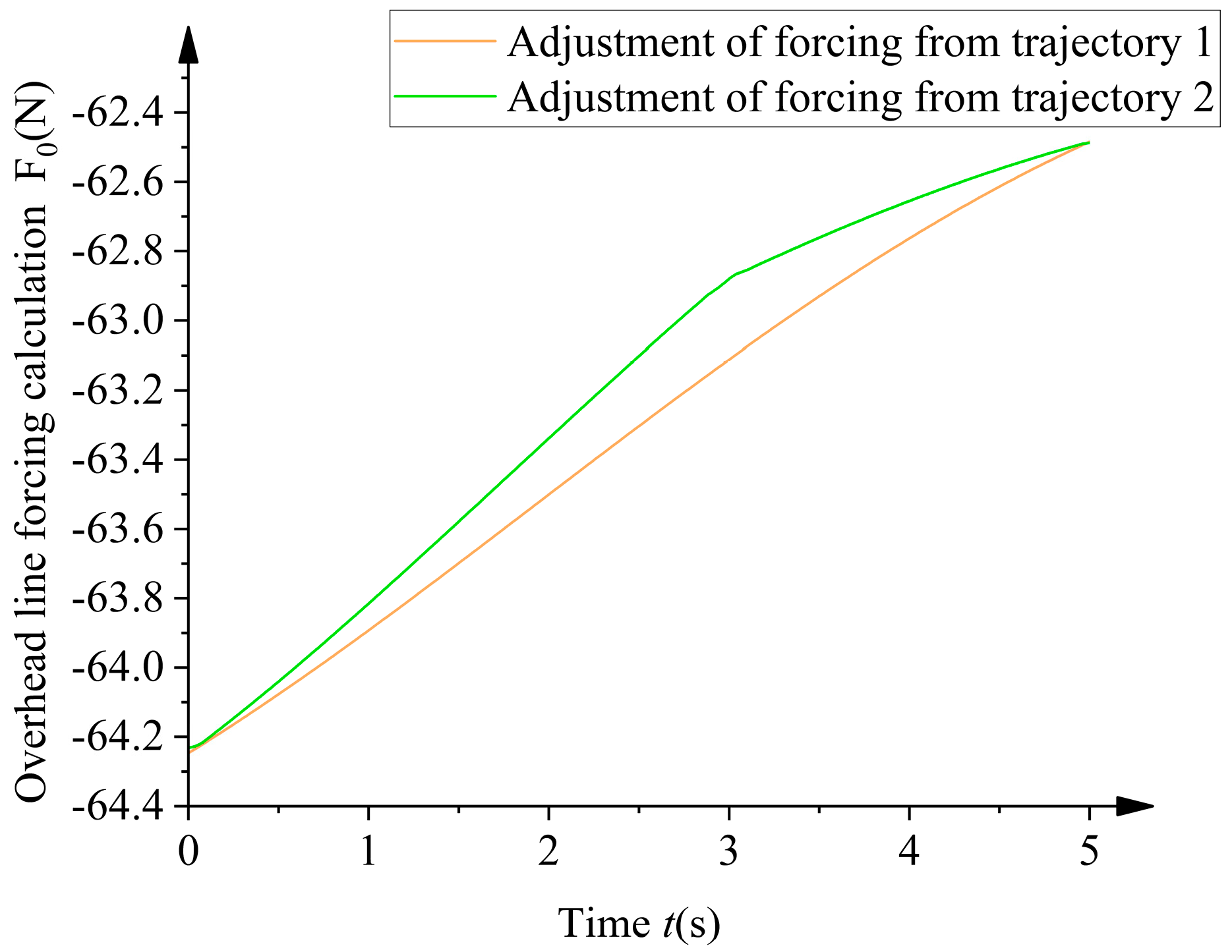
This study applies Newton’s third law and forced vibration theory to analyze the relationship between the robotic arm’s motion trajectory and the overhead line’s vibration response. Based on the response of the rigid–flexible coupling dynamics model, two active compensation joint trajectories are proposed to ensure the robot’s motion accuracy.

(3)

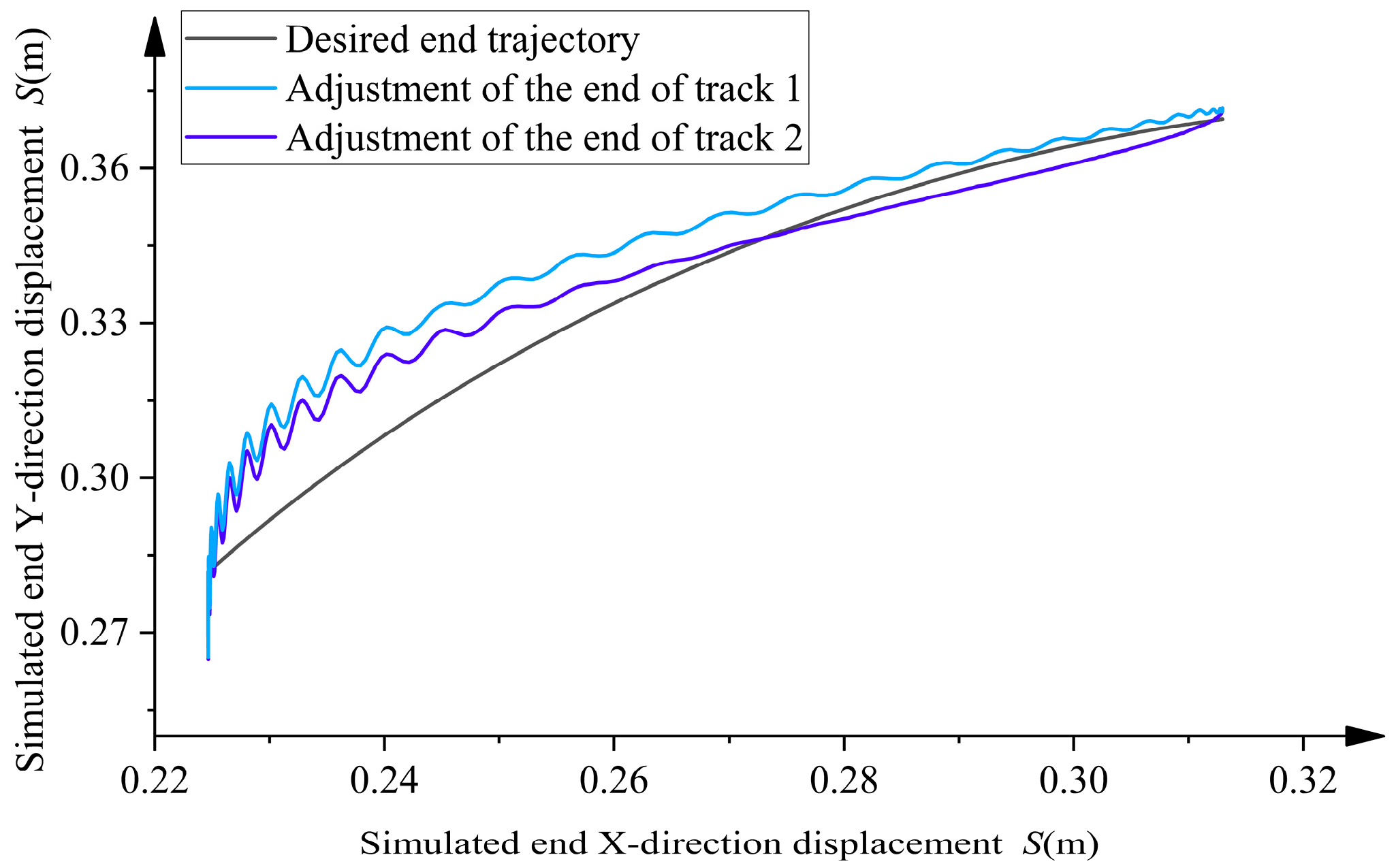
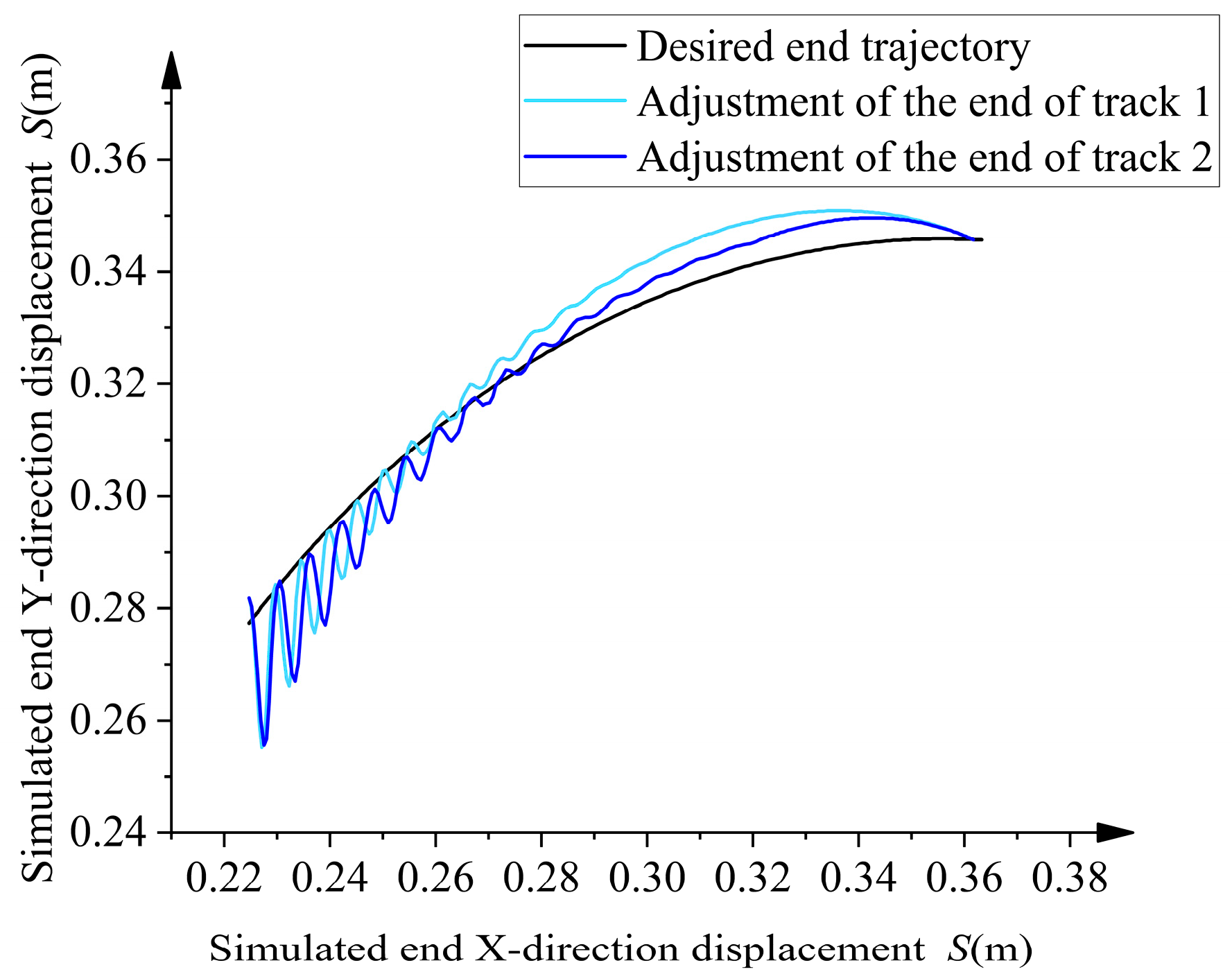
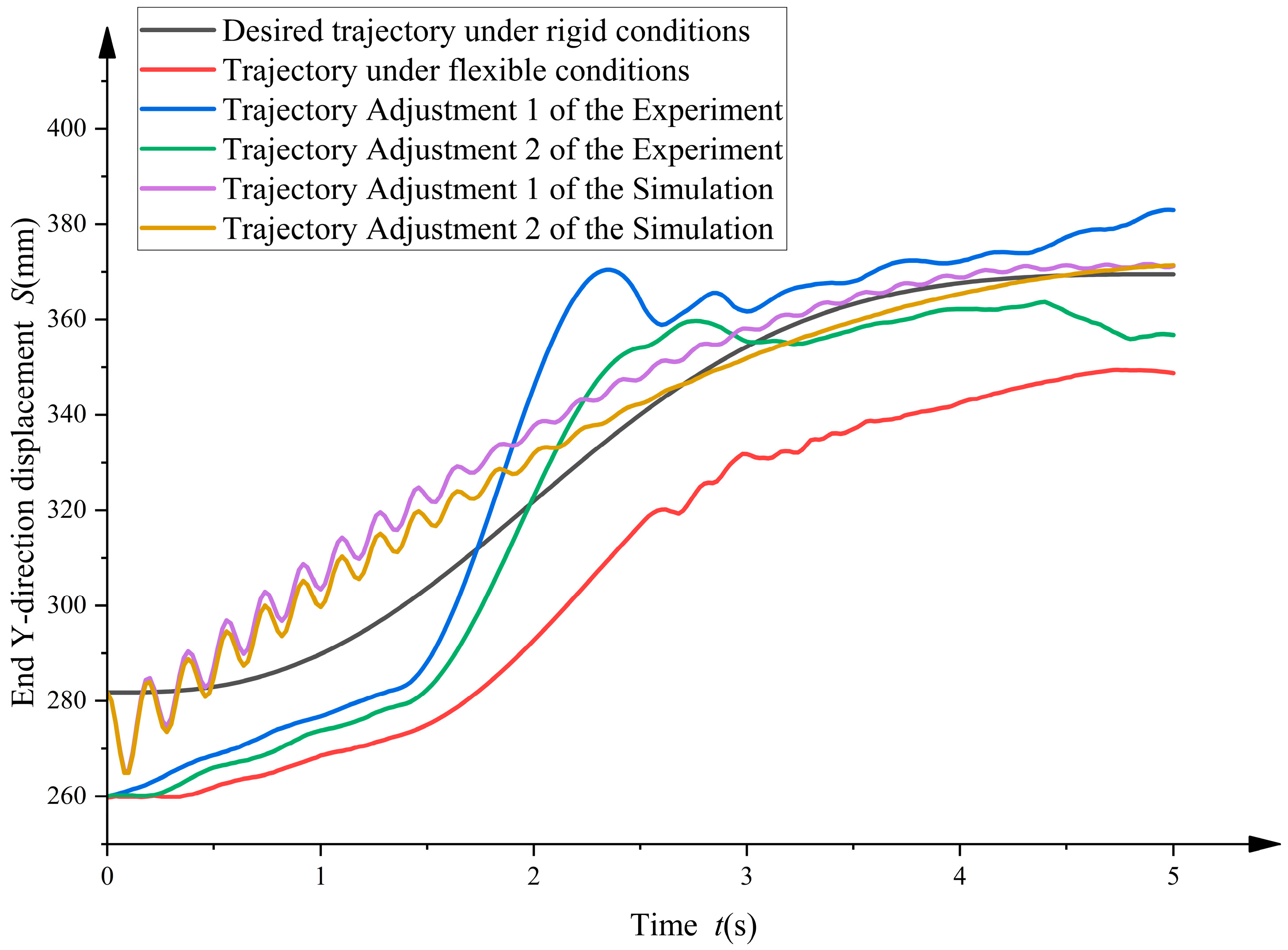
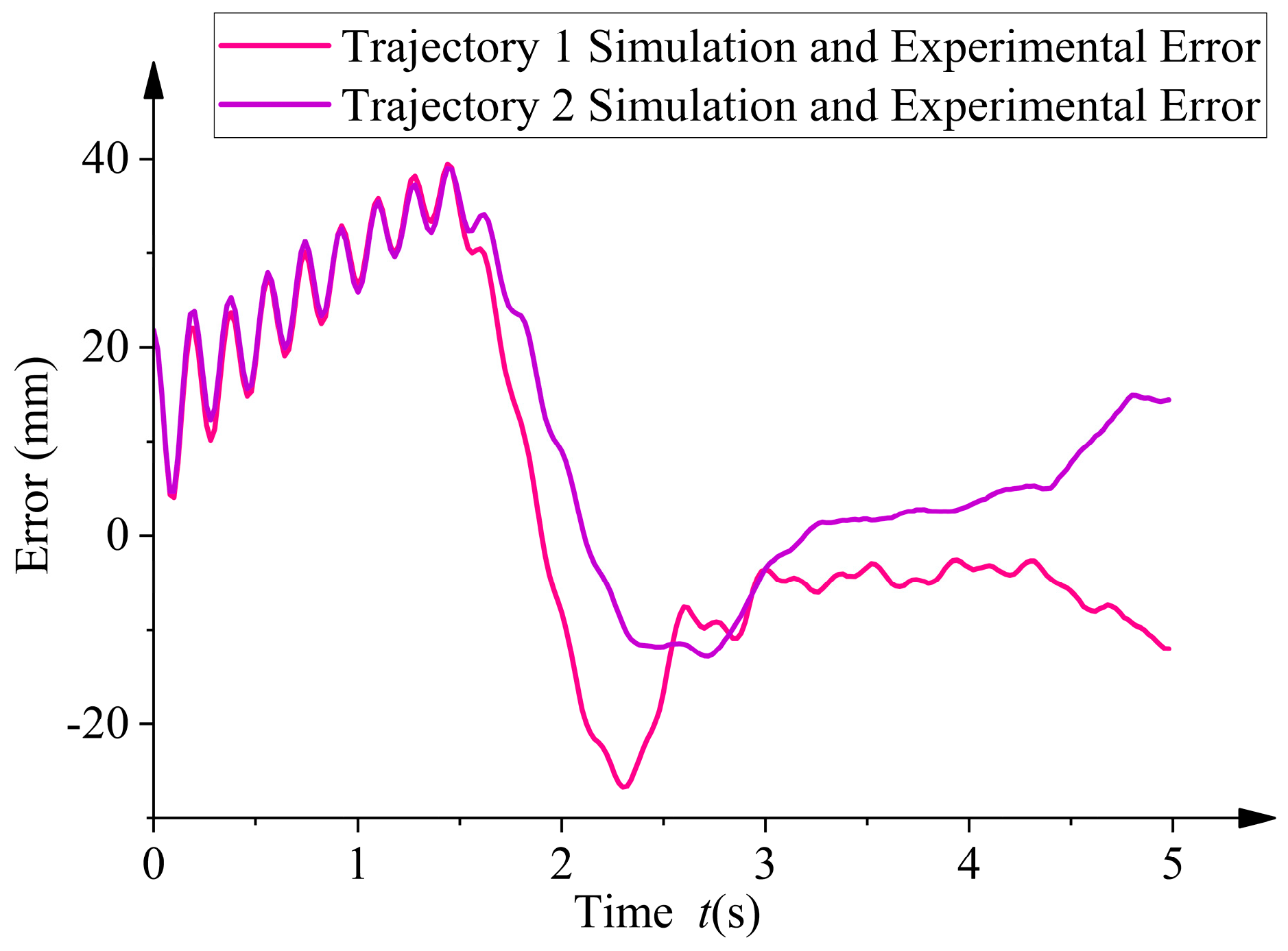
By comparing simulation and experimental analyses, the results show that on a two-meter-span overhead line, the average error of trajectory adjustment 2 is reduced by 2.1 times compared to the original trajectory. Additionally, as shown in Figure 28, trajectory adjustment 2 is closer to the ideal trajectory than trajectory adjustment 1. This not only validates the effectiveness of the rigid–flexible coupling dynamics model but also demonstrates the practical feasibility of the model selection and optimization method.

Limitations and Future Work: (1) This study verified the effectiveness of the trajectory compensation method for 2 m and 10 m overhead lines. The 2 m platform has been tested. Due to site limitations, the 10 m platform has not been built yet. Future work will focus on extending the setup to longer spans to address deformation and vibration issues. (2) Biomimetic methods can provide insights for overcoming challenges in flexible environments. For example, the interaction between spiders and webs can be applied to optimize the robot’s interaction with overhead lines, enabling more efficient trajectory control and vibration reduction. (3) Future research may use adaptive control algorithms to analyze the energy interaction between the robot and the vibrating overhead line.

References

1. Kakou, P.; Bukhari, M.; Wang, J.; Barry, O. On the vibration suppression of power lines using mobile damping robots. Eng. Struct. 2021, 239, 112312. [Google Scholar] [CrossRef]
2. Xiao, X.; Wu, G.; Du, E.; Li, S. Impacts of flexible obstructive working environment on dynamic performances of inspection robot for power transmission line. J. Cent. South Univ. Technol. 2008, 15, 869–876. [Google Scholar] [CrossRef]
3. Zhang, M.; Zhao, G.; Li, J. Nonlinear Dynamic Analysis of High-Voltage Overhead Transmission Lines. Shock. Vib. 2018, 2018, 1247523. [Google Scholar] [CrossRef]
4. Yang, L.; Wang, Y.; Wei, L.; Chen, Y. Structural Flexibility Effect on Spaceborne Solar Observation System’s Micro-Vibration Response. Aerospace 2024, 11, 65. [Google Scholar] [CrossRef]
5. Wei, Y.; Zhang, J.; Fang, L.; Li, C. Walking Characteristics of Dual-Arm Inspection Robot with Flexible-Ca using ble. J. Robot. 2021, 2021, 8885919. [Google Scholar] [CrossRef]
6. Fang, L.; Wei, Y.; Tao, G. Design of a Novel Dual-arm Inspection Robot with Flexible Cable. Robot 2013, 35, 319. [Google Scholar] [CrossRef]
7. Gonçalves, R.S.; Carvalho, J.C.M. A mobile robot to be applied in high-voltage power lines. J. Braz. Soc. Mech. Sci. Eng. 2014, 37, 349–359. [Google Scholar] [CrossRef]
8. Xiao, S.; Wang, H.; Zhang, J. Design and analysis of a novel inspection robot mechanism with assistant arms. In Proceedings of the IEEE International Conference on Cyber Technology in Automation, Control, and Intelligent Systems, Chengdu, China, 19–22 June 2016; pp. 19–22. [Google Scholar] [CrossRef]
9. Shruthi, C.M.; Sudheer, A.P.; Joy, M.L. Dual arm electrical transmission line robot: Motion through straight and jumper cable. Automatika 2019, 60, 207–226. [Google Scholar] [CrossRef]
10. Feng, C.; Qian, R. Mechanism Design and Crawling Process Force Analysis of Inspection Robot for Power Transmission Lines. In Proceedings of the IEEE International Conference on Unmanned Systems (ICUS), Beijing, China, 17–19 October 2019; pp. 221–225. [Google Scholar]
11. Barry, O.; Zu, J.W.; Oguamanam, D.C.D. Forced Vibration of Overhead Transmission Line: Analytical and Experimental Investigation. J. Vib. Acoust. 2014, 136, 041012. [Google Scholar] [CrossRef]
12. Li, X.; Fan, X.; Shang, D.; Peng, J. Dynamic performance analysis based on the mechatronic system of power transmission line inspection robot with dual-arm. Proc. Inst. Mech.Eng. Part C J. Mech. Eng. Sci. 2023, 237, 5391–5408. [Google Scholar] [CrossRef]
13. Jiang, W.; Shi, Y.; Zou, D.; Zhang, H.; Li, H.J. Research on mechanism configuration and dynamic characteristics for multi-split transmission line mobile robot. Ind. Robot. Int. J. Robot. Res. Appl. 2021, 49, 200–211. [Google Scholar] [CrossRef]
14. Zheng, X.; Wu, G.; Jiang, W.; Fan, F.; Zhu, J. Rigid–flexible coupling dynamics with contact estimator for robot/PTL system. Proc. Inst. Mech. Eng. Part K J. Multi-Body Dyn. 2020, 234, 635–649. [Google Scholar] [CrossRef]
15. Yang, D.; Feng, Z.; Ren, X.; Lu, N. A novel power line inspection robot with dual-parallelogram architecture and its vibration suppression control. Adv. Robot. 2014, 28, 807–819. [Google Scholar] [CrossRef]
16. Yang, D.; Feng, Z.; Zhang, X. A novel tribrachiation robot for power line inspection and its inverse kinematics analysis. In Proceedings of the IEEE/ASME (AIM) International Conference on Advanced Intelligent Mechatronics, Kaohsiung, Taiwan, 11–14 July 2012; pp. 502–507. [Google Scholar] [CrossRef]
17. Wang, W.; Bai, Y.; Wu, G.; Li, S.; Chen, Q. The Mechanism of a Snake-Like Robot’s Clamping Obstacle Navigation on High Voltage Transmission Lines. Int. J. Adv. Robot. Syst. 2013, 10, 330. [Google Scholar] [CrossRef]
18. Fan, W.; Zhang, S.; Zhu, W.; Zhu, H. An efficient dynamic formulation for the vibration analysis of a multi-span power transmission line excited by a moving deicing robot. Appl. Math. Model. 2022, 103, 619–635. [Google Scholar] [CrossRef]
19. Liu, B.; Zhang, C. Nonfragile Observer-Based Control With Passivity and H∞ Performance for a Class of Power-Line Inspection Robots With Input Time-Delay. IEEE Access 2024, 12, 102893–102903. [Google Scholar] [CrossRef]
20. Zhao, Z.; Wen, S.; Li, F.; Zhang, C. Free vibration analysis of multi-span Timoshenko beams using the assumed mode method. Arch. Appl. Mech. 2018, 88, 1213–1228. [Google Scholar] [CrossRef]
21. Zhang, L.; Fan, W.; Chen, Z.; Ren, H. Dynamics modeling and attitude-vibration hybrid control of a large flexible space structure. J. Vib. Control. 2024, 31, 555–568. [Google Scholar] [CrossRef]
22. Wu, C.; Lu, Z.; Yu, S.; Zheng, H. A modeling scheme for flexible manipulators by sublinks and passive joints. Robot 2000, 22, 344–349. [Google Scholar]
23. Hu, H.; Li, E.; Zhao, X.; Liang, Z.; Yu, W. Modeling and simulation of folding-boom aerial platform vehicle based on the flexible multi-body dynamics. In Proceedings of the International Conference on Intelligent Control and Information Processing (ICICIP), Dalian, China, 13–15 August 2010; pp. 798–802. [Google Scholar]
24. Gao, Z.; Yun, C.; Bian, Y. Coupling Effectof Flexible Joint and Flexible Link on Dynamic Singularity of Flexible Manipulator. Chin. J. Mech. Eng. 2008, 21, 9–12. [Google Scholar] [CrossRef]
25. Liu, Z.-y.; Hong, J.-z.; Cai, G.-p. A new dynamic model for a flexible hub-beam system. J. Shanghai Jiaotong Univ. (Sci.) 2009, 14, 245–251. [Google Scholar] [CrossRef]
26. Zarafshan, P.; Moosavian, S.A.A. Manipulation control of a space robot with flexible solar panels. In Proceedings of the IEEE/ASME (AIM) International Conference on Advanced Intelligent Mechatronics, Montreal, QC, Canada, 6–9 July 2010; pp. 1099–1104. [Google Scholar]
27. Heidari, H.R.; Korayem, M.H.; Haghpanahi, M.; Batlle, V.F. A new nonlinear finite element model for the dynamic modeling of flexible link manipulators undergoing large deflections. In Proceedings of the International Conference on Mechatronics (ICM), Istambul, Turkey, 13–15 April 2011; pp. 375–380. [Google Scholar]
28. Kermanian, A.; Kamali E, A.; Taghvaeipour, A. Dynamic analysis of flexible parallel robots via enhanced co-rotational and rigid finite element formulations. Mech. Mach. Theory 2019, 139, 144–173. [Google Scholar] [CrossRef]
29. Halim, D.; Luo, X.; Trivailo, P.M. Decentralized vibration control of a multi-link flexible robotic manipulator using smart piezoelectric transducers. Acta Astronaut. 2014, 104, 186–196. [Google Scholar] [CrossRef]
30. Zhu, L.; Lu, B.; Cheng, L.; Zheng, S.; Hao, J. Rigid-Flexible Coupled Robot Simulation and Vibration Analysis. Chin. J. Mech. Eng. 2015, 13, 120–123. [Google Scholar] [CrossRef]
31. Wang, Y.G.; Yu, H.D.; Xu, J.K. Design and Simulation on Inspection Robot for High-Voltage Transmission Lines. Appl. Mech. Mater. 2014, 615, 173–180. [Google Scholar] [CrossRef]
32. Zhang, X.; Wang, C.; Guo, K.; Sun, M.; Yao, Q. Dynamics modeling and characteristics analysis of scissor seat suspension. J. Vib. Control. 2015, 23, 2819–2829. [Google Scholar] [CrossRef]
33. Sharifnia, M.; Akbarzadeh, A. Dynamics and vibration of a 3-PSP parallel robot with flexible moving platform. J. Vib. Control. 2014, 22, 1095–1116. [Google Scholar] [CrossRef]
34. Srinil, N.; Rega, G.; Chucheepsakul, S. Three-dimensional non-linear coupling and dynamic tension in the large-amplitude free vibrations of arbitrarily sagged cables. J. Sound Vib. 2004, 269, 823–852. [Google Scholar] [CrossRef]
35. Xia, D. Research on Dynamics and Reliability of Heavy Cable Crane Aerial Ropeway Systems in Hydropower Engineering. Ph.D. Thesis, Wuhan University, Wuhan, China, 2013. [Google Scholar]
36. Avramov, K.V. Analysis of forced vibrations by nonlinear modes. Nonlinear Dyn. 2007, 53, 117–127. [Google Scholar] [CrossRef]
37. Zhao, N.; Jia, S.; Zhu, Z.; Huang, X.; Xiao, W.; Wang, X. Direct convolution integration method for random vibration analysis of structures subjected to nonuniformly modulated nonstationary excitations. Mech. Syst. Signal Process. 2022, 178, 109294. [Google Scholar] [CrossRef]
38. Ge, X.; Lei, Y.; Hou, X.; Lu, S.; Wang, J. Analysis of Mechanical Characteristics of Ice-Covered Conductor Galloping in Transmission Lines. Jiangxi Electr. Power 2019, 43, 33–38. [Google Scholar]
39. Yang, J.; Zhang, Q.; Xu, C.; Cui, H. Analysis of Bending Deformation in Simply Supported Beams under Longitudinal and Transverse Loads. Jiangxi Sci. 2015, 33, 733–735. [Google Scholar]
40. Chen, Y.; Guo, Y.; Zheng, T. Research on Automatic Shovel Trajectory and Trajectory Error Compensation for Loaders. Coal Mine Mach. 2024, 45, 33–36. [Google Scholar] [CrossRef]
Figure 1. Robot movement over obstacles.
Aerospace 12 00378 g001
Figure 2. Robot kinematics coordinates.
Aerospace 12 00378 g002
Figure 3. Trajectory planning: (a) joint position, (b) joint velocity, (c) joint acceleration.
Aerospace 12 00378 g003
Figure 4. Sketch of the robot structure.
Aerospace 12 00378 g004
Figure 5. Dynamic model and simulation results: (a) simulation model, (b) theoretical calculated torque, (c) simulation torque.
Aerospace 12 00378 g005
Figure 6. Schematic diagram of overhead line sub-pole model.
Aerospace 12 00378 g006
Figure 7. Torque analysis diagram of the manipulator joint in the overhead line mobile robot: (a) schematic diagram of the torque in the robot forearm joint; (b) instantaneous torque of the robot forearm joint.
Aerospace 12 00378 g007
Figure 8. Forcing analysis diagram for overhead lines.
Aerospace 12 00378 g008
Figure 9. 2 m Overhead Line End Trajectories under Rigid and Flexible Conditions.
Aerospace 12 00378 g009
Figure 10. Y-direction trajectory of the front arm end under a 2 m overhead line.
Aerospace 12 00378 g010
Figure 11. Joint trajectory adjustment of the robot under a 2 m overhead line: (a) The first set of joints to adjust the movement trajectory; (b) the second set of joints to adjust the movement trajectory.
Aerospace 12 00378 g011
Figure 12. Forcing forces generated by two adjusted trajectories under a 2 m overhead line.
Aerospace 12 00378 g012
Figure 13. Response Calculation of the 2 m Overhead Line System Dynamics.
Aerospace 12 00378 g013
Figure 14. End trajectories of two adjusted trajectories under a 2 m overhead line.
Aerospace 12 00378 g014
Figure 15. 10 m Overhead Line End Trajectories under Rigid and Flexible Conditions.
Aerospace 12 00378 g015
Figure 16. Y-direction trajectory of the front arm end under a 10 m overhead line.
Aerospace 12 00378 g016
Figure 17. Joint trajectory adjustment of the robot under a 2 m overhead line: (a) The first set of joints to adjust the movement trajectory; (b) the second set of joints to adjust the movement trajectory.
Aerospace 12 00378 g017
Figure 18. Forcing forces generated by two adjusted trajectories under a 2 m overhead line.
Aerospace 12 00378 g018
Figure 19. Simplified diagram of overhead line sag.
Aerospace 12 00378 g019
Figure 20. Sag of the overhead line at different positions of the robot.
Aerospace 12 00378 g020
Figure 21. End trajectories of two adjusted trajectories under a 10 m overhead line.
Aerospace 12 00378 g021
Figure 22. Overhead line mobile robot structure and hardware composition.
Aerospace 12 00378 g022
Figure 23. Overhead line damping measurements: (a) experimental environment setup for overhead lines; (b) spring–damping simulation system mode; (c) free vibration acceleration curves for overhead lines under heavy loads; (d) simulation curves for single-degree-of-freedom spring–damping system under heavy loads.
Aerospace 12 00378 g023
Figure 24. Effect of virtual damping coefficient and spring constant on the system’s vibration response: (a) the effect of virtual damping coefficient on the system’s vibration response; (b) the effect of spring constant on the system’s vibration response.
Aerospace 12 00378 g024
Figure 25. Diagram of the initial state of the device.
Aerospace 12 00378 g025
Figure 26. Experimental procedure.
Aerospace 12 00378 g026
Figure 27. Schematic diagrams of the experimental ends: (a) end horizontal direction X2; (b) end vertical direction Y2.
Aerospace 12 00378 g027
Figure 28. End Y-direction displacement.
Aerospace 12 00378 g028
Figure 29. Comparison of experimental and simulation errors.
Aerospace 12 00378 g029