Article

Efficient Adaptive Robust Aerodynamic Design Optimization Considering Uncertain Inflow Variations for a Diffusion Airfoil Across All Operating Incidences

1
Test Center, National University of Defense Technology, Xi’an 710106, China
2
School of Power and Energy, Northwestern Polytechnical University, Xi’an 710072, China
*
Authors to whom correspondence should be addressed.
These authors contributed equally to this work.
Aerospace 2025, 12(4), 341; https://doi.org/10.3390/aerospace12040341
Submission received: 13 February 2025 / Revised: 11 April 2025 / Accepted: 11 April 2025 / Published: 14 April 2025
(This article belongs to the Section Aeronautics)

Abstract

:
The random fluctuations in inlet flow represent a common uncertainty in aero-engine compressors, necessitating the control of its effects through blade optimization design. To account for the impact of inlet flow fluctuations on performance in blade design optimization, an efficient multi-objective adaptive robust aerodynamic design optimization (ARADO) method is proposed. The optimization method employs a novel sparse polynomial chaos expansion (PCE) and the advanced noisy Gaussian process regression (NGPR) technique is used to establish an initial stochastic surrogate model (SSM) containing statistical moments of aerodynamic performance. By introducing advanced sparse signal processing concepts, the sparce PCE significantly enhances the efficiency of acquiring each training sample for SSM. During the optimization process, the initial SSM autonomously updates based on historical optimization data, without requiring high precision across the entire design space. Compared to traditional model-based aerodynamic robust optimizations, the proposed ARADO method exhibits a faster convergence speed and achieves a superior average level of the optimal solution set. It also better balances various optimization objectives, concentrating the space distribution of optimal solutions closer to the average level. Ultimately, the ARADO is applied to the aerodynamic robust design of a high-load compressor airfoil across all operating incidences. The optimization results enhance aerodynamic performance while reducing performance diversity, thus aligning more closely with practical engineering requirements. Through data analysis of the optimal solutions, robust design guidelines for blade aerodynamic shapes are obtained, along with insights into the flow mechanisms that enhance aerodynamic robustness.

1. Introduction

The compressor, a crucial component of aircraft engines, significantly impacts overall efficiency. Uncertain factors, like blade geometric errors during the manufacturing process [1,2] and flow fluctuations at the inlet of compressors during operation [3,4], have raised concerns about aerodynamic performance. Optimizing the tolerances of sensitive geometric error parameters can mitigate the uncertain effects of manufacturing errors effectively. However, aerodynamic shape optimization of compressor blades is typically necessary to control performance variations caused by flow fluctuations. Traditional deterministic aerodynamic design optimization (DADO) may lead to subpar results by neglecting uncertainties [5]. When optimal solutions are highly sensitive to uncertainties, a significant performance dispersion becomes inevitable. Embracing robust aerodynamic design optimization (RADO) offers a more attractive strategy [6,7,8] by considering uncertain parameter effects.
RADO aims to optimize mean performance and minimize performance variability in a defined range simultaneously. The core of RADO involves quantifying uncertainties to determine both the mean and variance of performance changes caused by fluctuations in flow variables, a process referred to as uncertainty quantification (UQ). UQ relies on a substantial number of random samples for statistical analysis. In turbomachinery, three commonly used aerodynamic UQ methods include direct Monte Carlo (DMC) [9,10], sensitivity-based approaches [11,12], and polynomial chaos expansion (PCE) [13,14]. Sensitivity-based methods, along with PCE, can notably reduce computational fluid dynamics (CFD) costs for precise UQ compared to DMC. The sensitivity methods face challenges in accurately quantifying the impact of large-scale uncertainties including flow variations [15]. However, while classical PCE offers global characteristics, the computational expenses for CFD rise notably with the nonlinear order of flow variables. Therefore, a key to improving RADO efficiency lies in refining the accuracy and efficiency of aerodynamic UQ techniques.
In recent times, RADO has found application in domains such as the design of aerodynamic shapes for turbomachinery [16,17,18,19,20] and aircraft [21,22]. Analogous to DADO, RADO can be categorized according to optimization principles into gradient-based and surrogate model-based optimization methodologies. Gradient-based RADO (G-RADO) techniques [16] hinge on the sensitivity of aerodynamic UQ outcomes to design shape variables, employing optimization search strategies including steepest descent, conjugate gradient, and quasi-Newton methods. The fundamental approach entails acquiring the statistical moments (mean and standard deviation) of aerodynamic performance PCE, in conjunction with sensitivity analysis obtained through finite differences or adjoint methods. For instance, Luo et al. [17] utilized PCE to derive statistical moments of aerodynamic losses, and the first-order sensitivity of aerodynamic loss statistical moments concerning design shape variables. They applied the steepest descent method to improve the robustness of aerodynamic losses, accounting for airflow angle fluctuations in a turbine blade. Similarly, Zhang et al. [20] integrated PCE and discrete adjoint methods to conduct robust aerodynamic optimization for a two-dimensional turbine blade, suppressing the impact of inflow angle uncertainty. Nevertheless, even though gradient algorithms exhibit faster convergence, the optimization outcomes are susceptible to local optima.
Surrogate model-based RADO (SM-RADO) methods [21,22,23,24,25] can effectively address local optima challenges through the training of a precise stochastic surrogate model (SSM), which contains the statistical moments of aerodynamic performance obtained from UQ. The trained SSM can be enhanced using genetic algorithms [26], particle swarm [27], or simulated annealing [28] for optimization purposes. For instance, Zhao [21] utilized a Gaussian process to construct an SSM, and then employed the multi-objective evolutionary algorithm for improving the natural laminar flow characteristics of a supercritical airfoil, under Mach number uncertainties. Fusi [22] constructed a multi-fidelity SSM and subsequently employed genetic algorithms to optimize the aerodynamic shape of a helicopter rotor blade under varying angles of attack and velocities, with the goal of enhancing the mean lift-to-drag ratio and minimizing its variance. However, the research on the SM-RADO of turbomachinery started relatively late. Wang et al. [23] applied a neural network-based robust optimization strategy to NASA Rotor 37 under flow uncertainty, demonstrating superior mean performance and reduced variability in robust design compared to deterministic methods. Gouttiere et al. [24] trained the tuned radial basis function network to search for the optimal solution, achieving the RADO of NASA Rotor 37 under inlet profile uncertainty. Gao et al. [25] employed a support vector machine alongside multi-objective genetic algorithms to mitigate blade sensitivity to fluctuations in random inlet airflow angles.
The application of SM-RADO methods in compressor engineering has shown promise, yet challenges persist, such as increased optimization costs and concerns about accuracy. Improving the efficiency and precision of optimization results is crucial. The present SM-RADO methods rely heavily on SSM, and a significant limitation is the potential for inaccurate model approximations that can impede convergence towards the true optimal solution during optimization algorithm iterations. Achieving precise modeling throughout the design space necessitates a substantial volume of training data. Therefore, there is a growing need for the development of more efficient RADO techniques.
Studies in RADO and aerodynamic UQ have incorporated stochastic variations in flow variables at the compressor inlet [15,23,24,25,29,30], such as Mach number and inflow angle. It demonstrates the importance of considering flow fluctuations at the inlet in RADO. In most instances, robust optimization designs considering uncertain flow variables focus on the performance robustness of a single operational condition. Because the design operating condition is the longest working condition of the compressor, maintaining strong performance robustness is important. However, dispersion in performance at off-design conditions exceeds that at the design ones, emphasizing the need to enhance aerodynamic robustness across all operating conditions. However, as mentioned earlier, the efficiency of high-quality robust optimization designs is constrained by the training efficiency of UQ techniques and SSM.
In the study, an adaptive aerodynamic robust optimization (ARADO) method is proposed to bolster the efficiency of robust design optimization. This adaptive approach prioritizes the accuracy of the SSM near optimal design points rather than throughout the entire design space. By strategically adding training points near the optimal solution set, a substantial reduction in the number of experimental points needed for model training can be achieved, simultaneously enhancing the superiority of robust optimization results. Meanwhile, given the computational costs associated with aerodynamic UQs, each training point of the SSM is assessed using a novel sparse PCE to further diminish optimization time. Finally, the proposed ARADO method is used to improve performance robustness considering inlet flow fluctuations for a high-load compressor airfoil, significantly enhancing both mean performance and performance dispersion across all operational incidence conditions. Through data analysis of the optimal solutions, robust design guidelines for blade aerodynamic shapes are derived and the flow mechanisms that enhance aerodynamic robustness are excavated.

2. Robust Optimization Design Methods

2.1. Mathematical Description of RADO

For typical aerodynamic optimization challenges, RADO aims to minimize the sensitivity of the objective to uncertain factors while optimizing the mean value. If aerodynamic performance metrics are described as a vector q = [q1, q2, …], it involves reducing both the mean vector μq = [ μ q 1 , μ q 2 , …] and the standard deviation vector σq = [ σ q 1 , σ q 2 , …]. The mathematical model is
Find :   x n Min :   μ q 1 x , ξ , σ q 1 x , ξ μ q 2 x , ξ , σ q 2 x , ξ Subject   to :   g x , ξ 0
where x = [x1, x2, …, xn] is the shape design variables, ξ = [ξ1, ξ2, …, ξd] denotes the uncertain variables, and g(x, ξ) represents constraints associated with design and uncertainty variables. RADO typically involves considering aerodynamic performance metrics for multiple operating conditions, making it a multi-objective optimization problem with far more than two optimization objectives.

2.2. Traditional RADO Methods

In general, RADO can be classified based on optimization principles into two methodologies: G-RADO and SM-RADO. Due to the tendency of G-RADO solutions to fall into local optima, SM-RADO is more commonly applied in the robust optimization design of compressors. Figure 1 illustrates the workflow of the typical SM-RADO method [21,25,31,32,33,34], which relies on training a high-precision SSM containing statistical features (μq, σq) of aerodynamic characteristics. The efficacy of utilizing an optimizer with the SSM for robust optimization largely hinges on the approximation accuracy of the model. Failure to ensure the model’s accuracy often leads to optimization designs failing to converge to the true optimum. To uphold high accuracy across the entire design space, a considerable number of training samples are typically required.
Due to the time-consuming nature of flow field simulations using CFD programs, the computational time required for the optimizer to call the SSM is significantly lower by comparison. For instance, in the case study utilized in this paper (Section 4), a single steady simulation typically takes around 8–10 min, while the total time required to use the optimizer to call SSM for convergent optimizations is only 1–2 min. Thus, most of the computational cost in SM-RADO stems from CFD simulations for flow field analysis. As shown in Figure 1, the total number of CFD simulations required for robust optimization (Ntotal) is equal to the product of the size of the aerodynamic shape training database (Nt) and the total number of CFD simulations invoked for UQ (NUQ), denoted as
N t o t a l = N t × N U Q

3. Adaptive Aerodynamic Robust Optimization Method

3.1. Noisy Gaussian Process Regression

The Gaussian process regression (GPR) model offers excellent flexibility and adaptability, showcasing strong approximation capabilities for nonlinear and multi-modal design spaces. By leveraging Bayesian modeling principles, GPR fits the function space of output variables. The fundamental concept involves describing the output variable y using a Gaussian model M GPR x :
y x M GPR x = β x T θ + ε x
where β(x) represents a series of basis functions, usually using linear polynomials or quadratic polynomials. Quadratic polynomials are employed in the paper. The coefficient vector θ is estimated to be using the least squares methods. ε(x) denotes a zero-mean stationary Gaussian random variable, with its covariance function controlling it. The covariance takes on various forms, and in the study, the radial basis function (RBF) is chosen for its broad applicability.
The GPR model interpolates the local variations in the response output using adjacent training samples, resulting in zero interpolation error at the training sample outputs. Therefore, when the training sample outputs are contaminated by noise (such as numerical fluctuations in CFD), the generalization ability of the GPR model becomes challenging to guarantee. During the design of experiments for training samples, there will inevitably be some extreme aerodynamic shapes, and the CFD of those will produce numerical fluctuations. Many aerodynamic optimization problems based on the GPR model or RBF neural networks overlook this crucial consideration [25,32,35,36]. To reduce the impact of this issue on optimization convergence, it is necessary to employ a surrogate model that can circumvent noise contamination.
Rasmussen and Williams [37] proposed a method called noisy GPR (NGPR) to address the problem of function regression when training samples are affected by noise contamination. The analytical expression of the NGPR model is
M NGPR x = M GPR x + ε = β x T θ + ε x + ε n
where εn represents an additional noise term that follows a zero-mean Gaussian distribution with ε n N 0 , n . n = σ n 2 I denotes the covariance matrix of the noise term. For all training samples, the noise variance σ n 2 is a constant, implying that the noise is an independent and identically distributed Gaussian process. The advantages of the NGPR modeling approach are demonstrated in detail in Appendix A.

3.2. New-Generation Multi-Objective Genetic Algorithm

Among the myriad evolutionary algorithms employed for multi-objective optimization, non-dominated sorting genetic algorithm II (NSGA-II) is a widely used and influential method. Since its inception, NSGA-II has evolved into a cornerstone algorithm in multi-objective optimization, renowned for its simplicity, efficiency, and distinct advantages. Presently, NSGA-II is the most widely used algorithm in optimization designs of turbomachinery [33,34,35,36].
While NSGA-II excels in solving bi-objective optimization problems, its crowding distance algorithm does not ensure a uniform distribution of Pareto solutions in the solution space for optimization problems with more than two objectives. As in Section 2.1, RADO typically involves considering aerodynamic performance metrics for multiple operating conditions, making it a multi-objective optimization problem with far more than two objectives. Therefore, using NSGA- II in RADO may result in low-quality Pareto solutions. However, the introduction of NSGA-III successfully addresses this issue by incorporating reference points to replace crowding distance [38]. Figure 2 shows the algorithm of NSGA-III. The effectiveness of NSGA-III is demonstrated in Appendix B.

3.3. Novel Sparse Polynomial Chaos Expansion

If ξ1, ξ2, …, ξd are independent random input variables, a random variable y can be expanded by
y = i = 1 a ^ i H i ξ
where PCE coefficients a ^ are real numbers and H indicates the PCE basis functions. There exists one-to-one correspondence between random distributions and basis functions [39,40]. In the L2 space, the basis function is a complete orthogonal basis that satisfies
H j ξ , H k ξ = δ j k
where δjk is the Delta function. In the applications, a limited number of polynomial chaos samples are reserved to approximately describe y according to the following truncation rule:
y i = 1 P a ^ i H i ξ , P = p + d ! p ! d !
where P is the number of the reserved polynomial chaos; p and d are the order of PCE and the number of random variables, respectively.
To construct the full PCE as in Equation (7), the unknown coefficients a ^ must be determined. Using N samples, the coefficient vector a ^ = [ a ^ 1 , a ^ 2 , , a ^ P ] T can be estimated by ordinary least squares:
a ^ = Ψ T Ψ 1 Ψ T Y
where Ψ denotes a matrix (N × P) with elements Ψij= Hj(ξ(i)) for i = 1, 2, …, N and j = 1, 2, …, P. Y is a vector of N dimension, in which the i-th element is y(ξ(i)). As suggested in ref. [41], when constructing the full PCE, at least N = 2P = 2(p + d)!/p!d! samples in low-discrepancy sequences [42] are selected, since they can give a better approximation at each polynomial order. It is observed that, as the dimension or nonlinear order of the input variable expands, the training expense associated with full PCE increases exponentially. Hence, this limitation significantly hinders the practical application of full PCE in engineering contexts.
However, not all PCE terms contribute significantly to the output response; most have negligible or zero contributions. Therefore, efficiently identifying and retaining only the coefficients of significant terms can greatly reduce computational costs. Such a reduced model is known as a sparse PCE. To accurately pinpoint the significant PCE terms and retain their coefficients, it is essential to leverage sparsity optimization techniques, which have been widely utilized in recent years in the field of information recovery.
Blatman [43] firstly exploited the least angle regression to detect the important PCE basis functions based on the correlation to the model output. Other sparsity optimization methods include compressive sensing [44] and weighted least squares [45], which have been applied to reduce the number of PCE construction samples. To decrease the number of necessary construction samples, orthogonal matching pursuit (OMP) [46] is applied in the study, based on which a novel sparse PCE can be implemented. The OMP algorithm is a linear regression tool that iteratively minimizes the norm of the approximation residual and then sets most undetermined coefficients to zero. The construction step of the proposed novel sparse PCE is shown in Figure 3. In Section 4.3, its advantage in construction efficiency will be illustrated.
Due to the orthogonality of Hi(ξ) shown in Equation (6), the mean and standard deviation of y can be evaluated using all non-zero coefficients in the novel sparse PCE:
μ y = a ^ 1
σ y = i = 2 a ^ i 2

3.4. Adaptive Aerodynamic Robust Design Optimization

During the optimization process, SSM typically does not necessitate high approximation accuracy across the entirety of the design space; instead, precision in the vicinity of the optimal solution is sufficient. Consequently, the paper introduces an adaptive strategy integrated into robust aerodynamic optimization, leading to the formulation of the ARADO method, illustrated in the flowchart presented in Figure 4.
Initially, the geometry of the compressor blade is parameterized, and appropriate parameters are selected as design variables for optimization. The design variables are perturbed to sample a few training blade geometries, which are then added to the aerodynamic shape training database. For each selected geometry, aerodynamic performance uncertainties are quantified using the proposed novel sparse PCE method, enabling the statistical characteristics (μq, σq) of aerodynamic performance with high CFD efficiency. Based on the blade shapes and their corresponding statistical characteristics, an initial NGPR model is established.
Subsequently, NSGA-III is employed to invoke the NGPR model for robust optimizations, obtaining the optimal blade set corresponding to the Pareto optimal solution set. The optimal blade set is integrated into the aerodynamic shape training database, and the NGPR model is updated by assessing their aerodynamic statistical characteristics using the introduced novel sparse PCE. It indicates that the training samples are automatically adjusted utilizing historical optimization data, progressively converging towards the optimal solutions. This adaptive approach necessitates the NGPR model to achieve precision solely near the optimal solutions, rather than requiring high accuracy across the entire design space. By introducing training points only in proximity to the optimal solution set, the number of training points needed for the NGPR model can be significantly reduced, thereby diminishing the total CFD numbers required for aerodynamic robust optimization.
ARADO consists of two specific loops. One is the internal iteration, which employs the NSGA-III to invoke the NGPR model for optimizations, seeking blades with optimal aerodynamic robustness. Another is the external iteration, which involves adding the optimal blades to the training database and utilizing the proposed novel sparse PCE to invoke CFD for aerodynamic UQ, thereby updating the NGPR model. There are two convergence criteria for external iteration. One is the approximation accuracy of the NGPR model to the Pareto optimal solution set, that is, the relative error between the surrogate model and CFD, εmodel, in consecutive iterations, is less than the threshold ε0.
ε m o d e l = f m o d e l f 2 f 2 ε 0
where f = [f1, f2, …] represents the CFD results of the optimization objectives, where f with the subscript “model” denotes the predicted results of the NGPR model. The second convergence criterion is that the relative error of the means of all objectives in the Pareto set, ε(EPareto(f)), in consecutive iterations, is less than the threshold ε0.
ε E P a r e t o f i = E P a r e t o f i E P a r e t o f i o l d E P a r e t o f i o l d ε 0
where the subscript “old” denotes the previous external iteration step. EPareto(fi) represents the mean of the objective fif at the current external iteration step.
E P a r e t o f i = j = 1 N a d a p t i v e f i j N a d a p t i v e
where Nadptive is the number of samples in the Pareto set at the current external iteration step. It is also the number of samples that are adaptively updated and added to the training database for the next external iteration step.
Note: the ARADO algorithm may take longer to optimize scalability to 3D or transient CFD problems, due to the increased computational resources required for single 3D and transient CFD simulations.
Due to the ARADO comprising both internal and external iterative processes, the total number of CFD computations required is
N t o t a l = N i n i t i a l + N u p d a t e d × N a d a p t i v e × N U Q
where Ninitial represents the number of aerodynamic shape samples used to train the initial NGPR model, and Nupdated denotes the number of updates for the NGPR model.

4. Mathematical Modeling of RADO Considering Inflow Random Fluctuations

4.1. Research Object and Numerical Schemes

The aerodynamic shape of a high subsonic compressor airfoil, specifically obtained from the mid-span section of the exit stage stator blade within a multi-stage high-load axial compressor [47], will be the focal point of this investigation. The pertinent design specifications of the airfoil can be found in Table 1. The operational conditions were established by evaluating the inflow conditions across various mass flow rates at the designated rotational speed of the compressor. Consequently, as the compressor undergoes throttling, the operational incidence (α) of the airfoil escalates, while the inlet becomes susceptible to stochastic fluctuations in aerodynamic variables like Mach number (Ma).
The numerical methodology employed encompassed the utilization of the NUMECA 13.2 software for solving the Reynolds-averaged Navier–Stokes (RANS) equation. The closure of the RANS equation was achieved through the adoption of the two-equation k-epsilon turbulence model. A single-passage cascade structured with an O4H mesh topology was utilized to model the flow structure. To maintain a maximum normalized wall distance y+ below 1, the initial cell size on the solid surface was established at 10−6 m. The mesh comprised approximately 160,000 elements, a quantity validated in Ref. [30] as adequate for evaluating the performance variations of subsonic compressor airfoils in response to minor inflow parameter adjustments.
Figure 5 depicts the layout and grid of the computational domain utilized in this investigation. The computational domain extended 1.0C upstream and 2.0C downstream of the blade row, respectively. The inlet boundary conditions were defined by a total pressure of 101,325 Pa, total temperature of 288.15 K, and an incidence angle. Conversely, the outlet boundary was characterized by a variable mass flow rate, facilitating the adjustment of the inlet Ma as necessary.

4.2. Aerodynamic Shape Parameterized Design and Numerical Validation

Figure 6 shows the scheme of the parameterized design. As shown in Figure 6a, all Bezier control points are divided into two parts from the middle of the chord, sparse near the middle length and dense at both ends of the airfoil. As shown in Figure 6b, a ninth-order Bezier curve with 10 control points is used to parametrically fit the camber. In the aerodynamic robust optimization, the control points at both ends of the airfoil kept constant, aiming at maintaining the stagger angle unchanged. A new airfoil shape is generated by varying the vertical distance between the middle 8 control points and the chord. These distances h2, h3, …, h9 in Figure 6b are the design variables for optimization. Table 2 provides the relative positions along the chord for the design variables.
To ensure the richness of design space in optimization, the range of variation for hi is set to ±20% of the original value hi,o, where i = 2, 3,…, 9. Figure 7 illustrates the airfoil shapes at the boundaries of the design variables. The blue dashed line represents the airfoil shape when all design variables are at the upper boundary, while the red dashed line represents the airfoil shapes when all optimization variables are at the lower boundary. When hi = hi,o, it corresponds to the original airfoil shape depicted by the black dashed line.
Figure 8 presents the numerical validation of the parameterized original airfoil, in which the total pressure loss coefficient ωexp and surface pressure coefficient BP on the experimental measurement plane can be calculated:
ω e x p = P t i n P t e x p P t i n P s i n
B P = P t i n P s P t i n P s i n
where Pt and Ps are the total and static pressures and subscripts in and exp denote the inlet and the experiment measurement location. The measurement plane was positioned at 0.5C downstream of the blade row, as shown in Figure 5a. The numerical results demonstrate a high level of agreement with the experimental data, confirming the accuracy of the aerodynamic shape parameterization, as well as the numerical schemes in capturing the aerodynamic performance and flow structure.
In the subsequent study, key aerodynamic performance metrics of interest included global total pressure loss coefficient ω and static pressure coefficient Cp:
ω = P t i n P t o u t P t i n P s i n
C p = P s o u t P s i n P t i n P s i n
where the subscript out represents the outlet of the computational domain. ω quantifies overall aerodynamic losses, while Cp quantifies the airfoil’s ability to diffusion airflow.

4.3. Uncertainty Quantification Method

Using the full PCE, proposed novel sparse PCE and DMC methods, aerodynamic UQ regarding the inlet Ma fluctuations was conducted for the original airfoil shape. The inlet Ma follows a Gaussian distribution with a mean of 0.6 and a standard deviation of 0.015 [48]. The DMC was performed 10,000 times to obtain reference values for the statistical moments of aerodynamic characteristics. For the full PCE, a minimum of 2(p + d)!/p!d! = 2(p + 1) samples were required to construct. By comparing with the DMC results, the order p required for utilizing PCEs for quantifying aerodynamic uncertainty was ascertained, validating the accuracy and efficiency of the novel sparse PCE.
At an operating incidence of 9°, aerodynamic UQ is exemplified. Table 3 displays the convergence behavior of the mean and standard deviation of global loss coefficient, μω and σω. It demonstrates the efficacy of both full and sparse third-order PCEs in approximating statistical properties. Notably, the latter’s efficiency is half that of the former. The standard deviation distribution of isentropic Mach number (Mais) near the suction spike is visualized in Figure 9, affirming the effectiveness of the sparse PCE method. From this, it can be concluded that at any operating incidence, the uncertainty impact of inlet Ma variations on aerodynamic performance and flow characteristics can be efficiently assessed by the proposed sparse PCE at third-order and four sample points.
Note: the robustness and efficiency of sparse PCEs may decrease with high-dimensional aerodynamic problems or more complex compressor blade geometries, but sparse PCEs still have outstanding advantages in terms of training sample size, which has been proven in the author’s previous studies [40,44].

4.4. Description of RADO Problem

In internal flows, fluctuations in the inlet Ma impact aerodynamic losses, blade loads, and boundary layer flows. Therefore, this study selects the typical source of inflow uncertainty, the Mach number, as the uncertain variable for the RADO of the high subsonic compressor airfoil, where Ma ~ Gaussian(0.6, 0.0152) [48].
For the original airfoil shape considering inlet Ma fluctuations, Figure 10 displays how μω and σω vary with the incidence α. “Nominal” represents the aerodynamic coefficients without inlet Ma fluctuations. Figure 10b indicates that under the influence of inlet Ma fluctuations, ω exhibits significant random variations at α = 9° or −8°, particularly pronounced at α = −8°. This analysis suggests that stochastic fluctuations in the inflow Ma primarily induce uncertainty effects on the global losses away from the design incidence, especially at negative incidences far from the design incidence.
Figure 11 illustrates how the mean and standard deviation of static pressure coefficient, μ C p and σ C p , vary with the incidence α. Unlike the ω behaviors, Cp exhibits significant fluctuations at the design incidence of α = 0° and positive incidence α = 4°, reaching its peak at α = 4°. Hence, inflow Ma fluctuations predominantly affect the static pressure coefficient near its design incidence. In comparison, ω is more sensitive to inflow Ma fluctuations, with the maximum of the relative fluctuation σ C p / μ C p reaching approximately 2.50% across the entire incidence range, while the maximum σω/μω reaches up to 6.09%.
The analysis of Figure 10 and Figure 11 suggests that in optimizing the aerodynamic robustness across all operating incidences, the optimization objectives can be streamlined to reducing both μω and σω at α = −8° or 9°. Further exploration was conducted to determine if the objectives could be simplified to minimize the statistical characteristics of ω at a single incidence. A total of 500 sets of new airfoil shapes were randomly perturbed and generated within the space of the design variables (h2, h3, …, h9). Based on these new shapes regarding inlet Ma fluctuations, Figure 12 presents the scatter plot of the statistical characteristics at α = −8° and 9°. Obviously, there is a strong negative correlation between the statistical characteristics at α = −8° and 9°. Therefore, simplifying the optimization objectives to focus solely on reducing the statistical characteristics at one operating incidence may lead to disproportionately high values at other incidences.
In summary, for the RADO of the studied compressor airfoil, the optimization objective is to simultaneously reduce four parameters: μω and σω at off-design incidences, α = −8° and α = 9°. In contrast to previous studies [17,25,33], the RADO considers both positive and negative operating incidences, thereby ensuring aerodynamic robustness across the full range of operating incidences, which is a distinctive innovation of this study. The mathematical model of the RADO can be summarized as follows:
Find :                         h = h 2 , h 3 , h 4 , h 5 , h 6 , h 7 , h 8 , h 9 8 Min :                         α = 8 ° : μ ω h , M a , σ ω h , M a α = 9 ° : μ ω h , M a , σ ω h , M a Subject   to :       h i , o 20 % h i , o h i h i , o + 20 % h i , o                                               α = 8 ° : μ ω h , M a μ ω , o α = 9 ° : μ ω h , M a σ ω , o
where μω,o and σω,o are the mean and standard deviation of ω for the original airfoil shape.

5. Results and Discussion

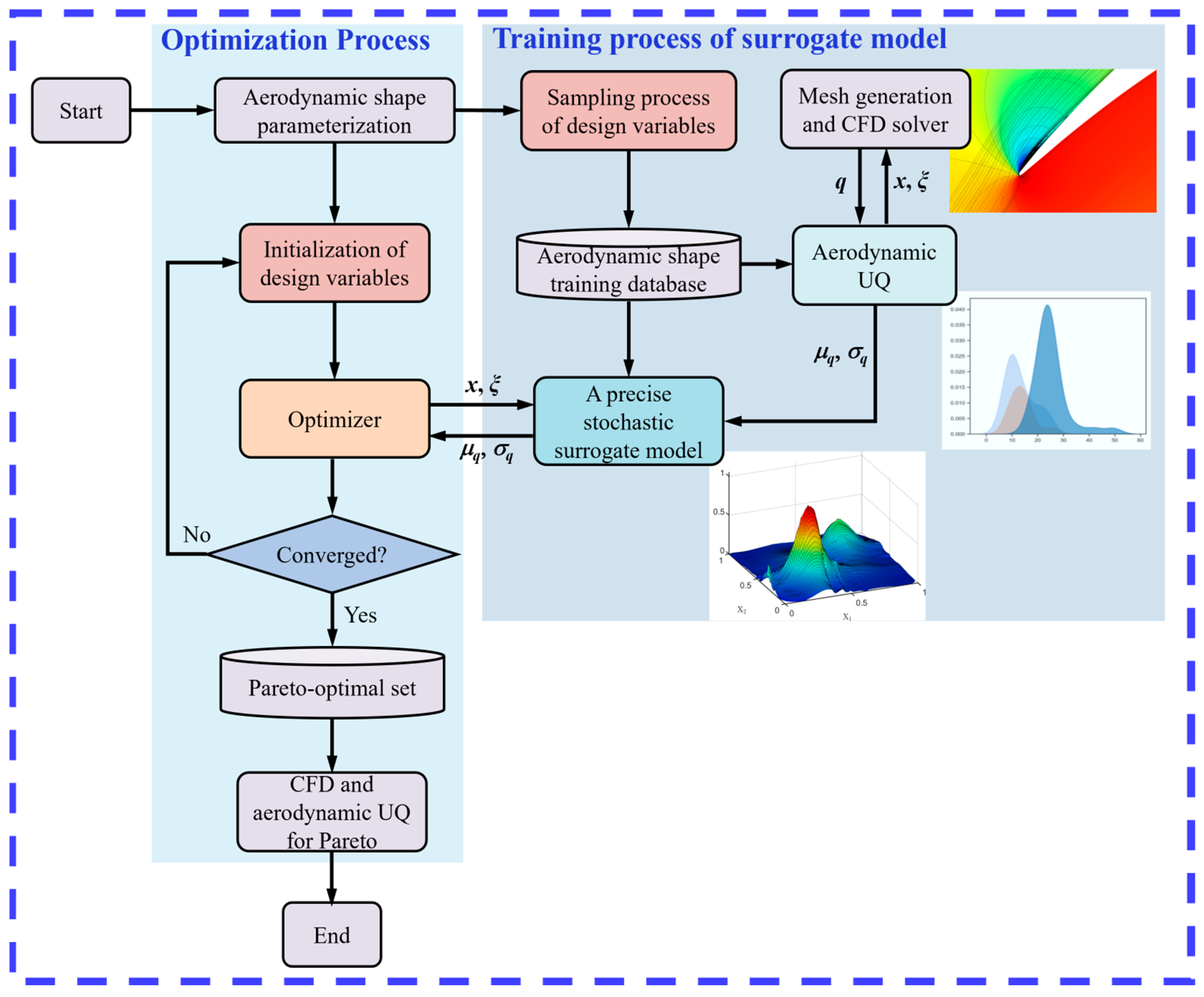
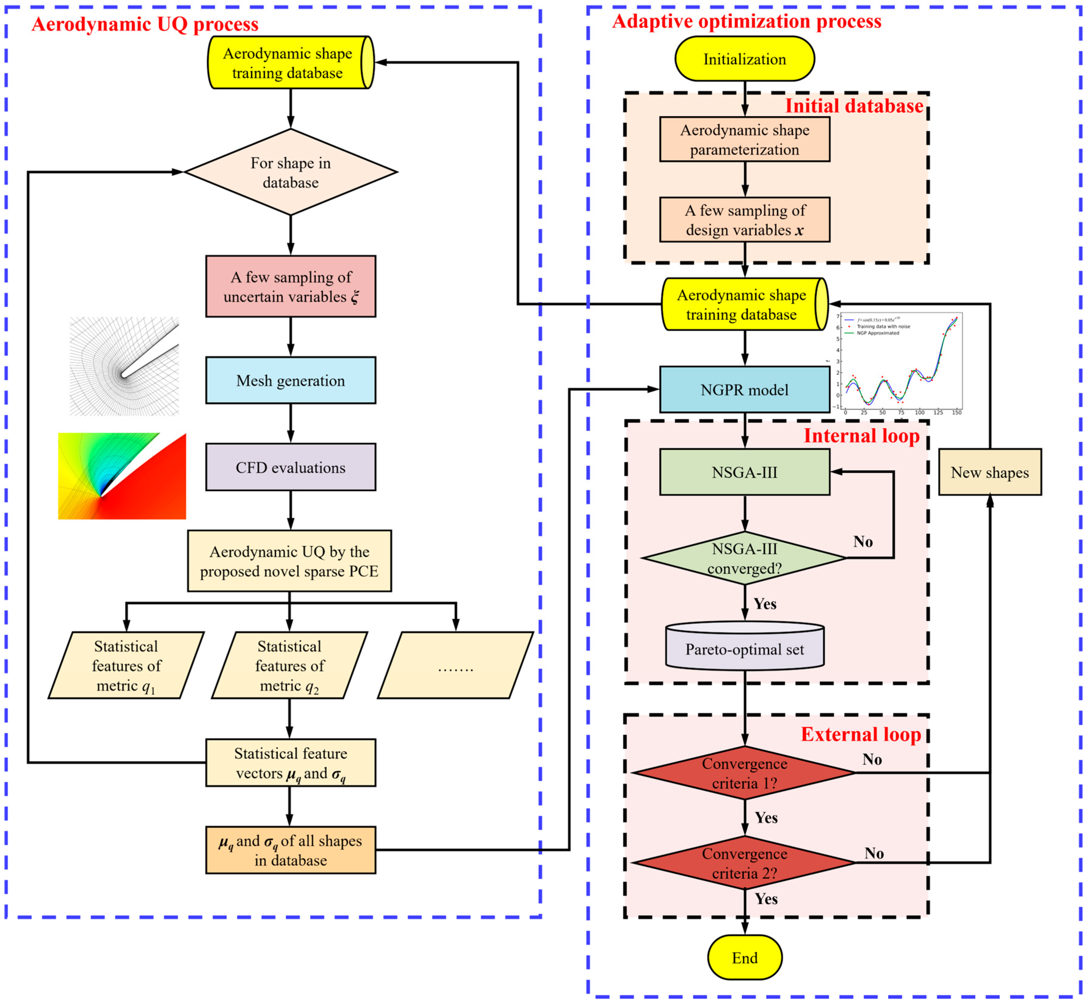
5.1. Verification of the Proposed ARADO Method

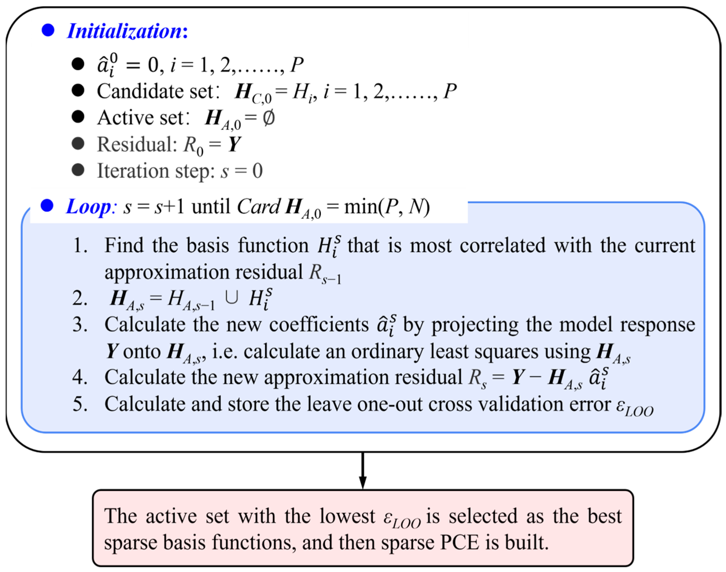
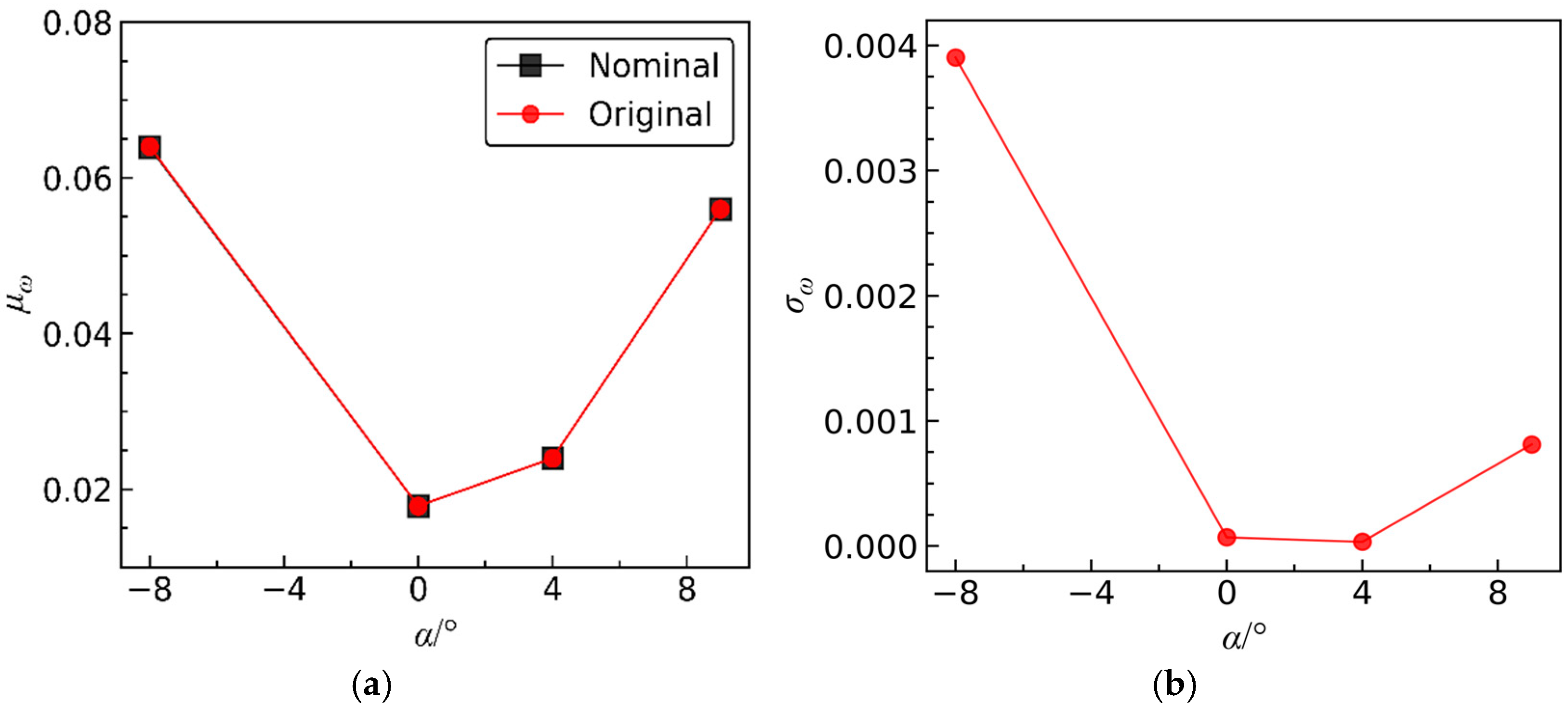
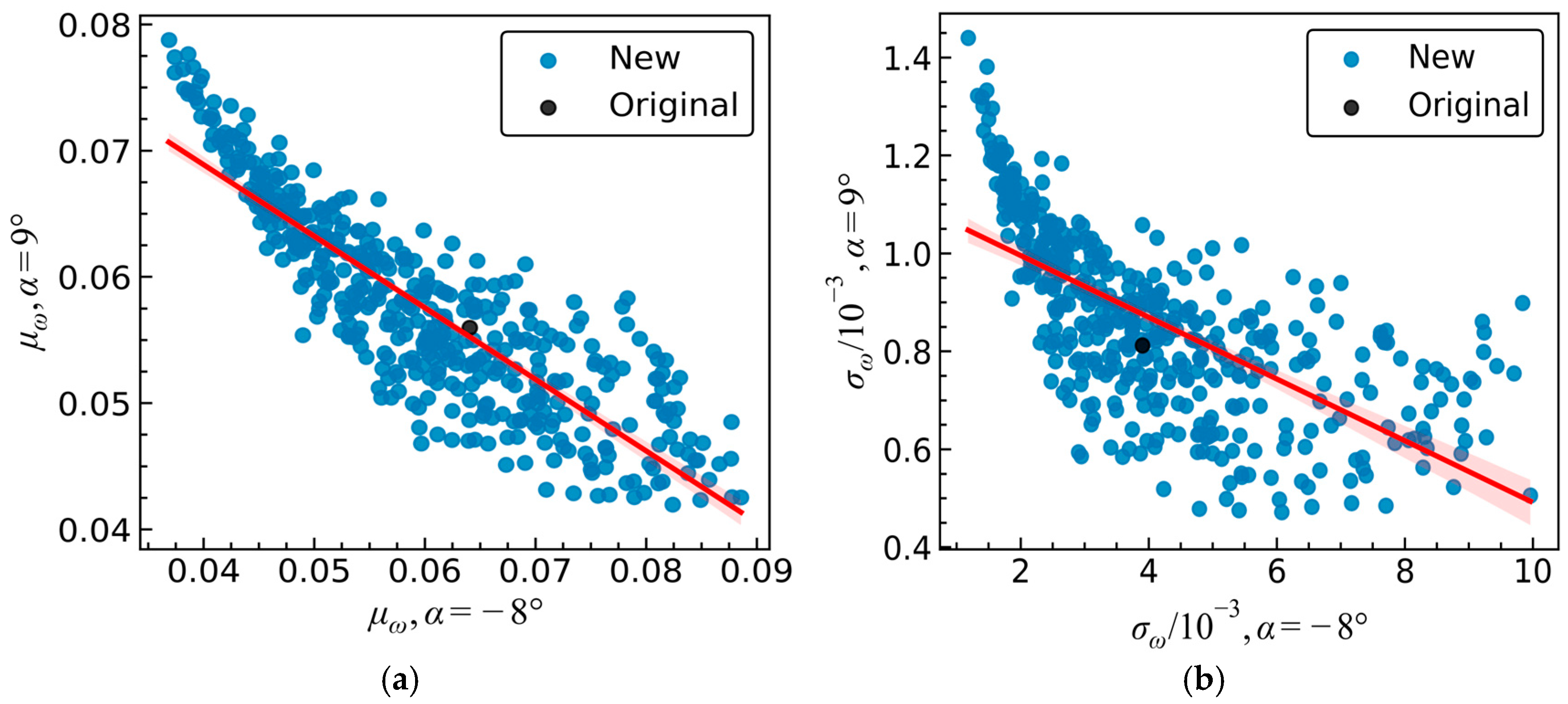
For the optimization problem described in Equation (19), the proposed ARADO method is employed for optimization. Prior to adaptive optimizations, an initial NGPR model with the training sample size set at Ninitial = 40 is constructed. Considering the uniformity of initial training samples, the low-discrepancy sequence sampling method is used. For each sample for training the NGPR model, the proposed sparse PCE is applied twice for aerodynamic UQs at the third polynomial order, yielding μω and σω at two operating incidences, α = −8° and 9°. This means that four CFDs are needed per single UQ, and the total number of CFDs for twice UQs, NUQ, is 8.
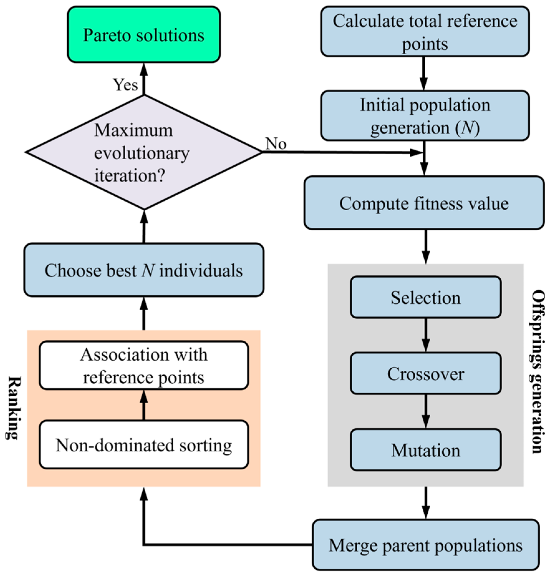
In addition, the parameters for the NSGA-III algorithm are set as follows: population size of 20, evolution generations of 1000, crossover rate of 0.9, and mutation rate of 0.1. Consequently, for each external iteration step of the optimization process, a Pareto-optimal solution set of size Nadaptive = 20 is obtained. The convergence threshold ε0 for the adaptive optimization is set at 1%.
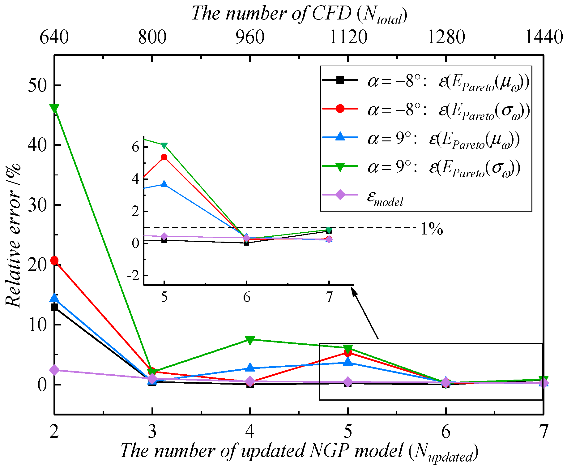
Figure 13 illustrates the external iteration process of the ARADO method. The figure reveals that the ARADO conducts a total of seven external iterations. After the seventh iterative step, the relative error εmodel remains within 1% across two consecutive iterative steps, which is below the specified convergence threshold ε0. This outcome confirms the accuracy of the constructed stochastic surrogate model in the vicinity of the Pareto-optimal solutions. Furthermore, it demonstrates that for α = −8° and 9°, both ε(EPareto(μω)) and ε(EPareto(σω)) are below the threshold of 1% in the sixth and seventh iterations, thereby meeting the prescribed iterative convergence criteria.
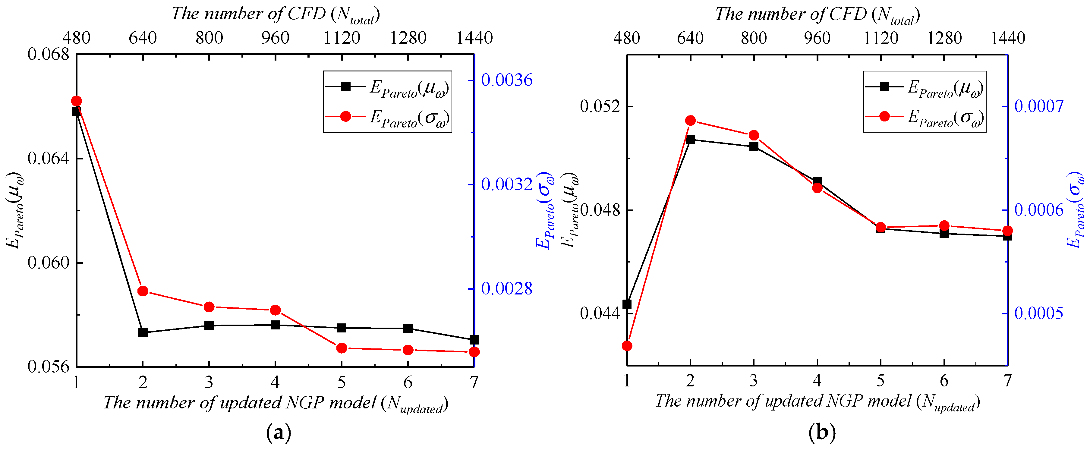
The variations of EPareto(μω) and EPareto(σω) with the number of external iteration steps are depicted in Figure 14. When Nupdated ≥ 5, the EPareto(μω) and EPareto(σω) for the two aforementioned operating incidences essentially stabilize, affirming the convergence of ARADO. The mean values EPareto(μω) and EPareto(σω) can reflect the overall level of Pareto. The ARADO method developed in this study yields EPareto(μω) and EPareto(σω) of 0.057046 and 0.002558, respectively, for α = −8°, and 0.046993 and 0.00057, respectively, for α = 9°. In terms of computational expenses, the entire aerodynamic robustness optimization required a total of 1440 CFD evaluations.
To highlight the superiority of the proposed ARADO method, a comparative optimization study was conducted with the SM-RADO method described in Section 2.2. In SM-RADO, the stochastic surrogate model and optimization algorithm also utilize the NGPR model and NSGA-III, with the NSGA-III parameters set as follows: a population size of 20, 1000 generations, crossover rate of 0.9, and mutation rate of 0.1. Four NGPR models are directly constructed using Nt = 100, 200, 300, and 500 training samples obtained from low-discrepancy sequences. Subsequently, NSGA-III is invoked for optimization with each model, followed by an analysis of the optimization results.
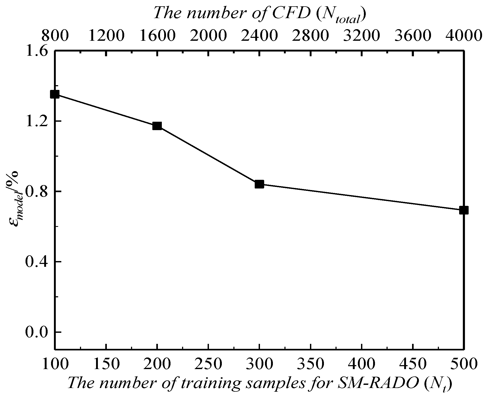
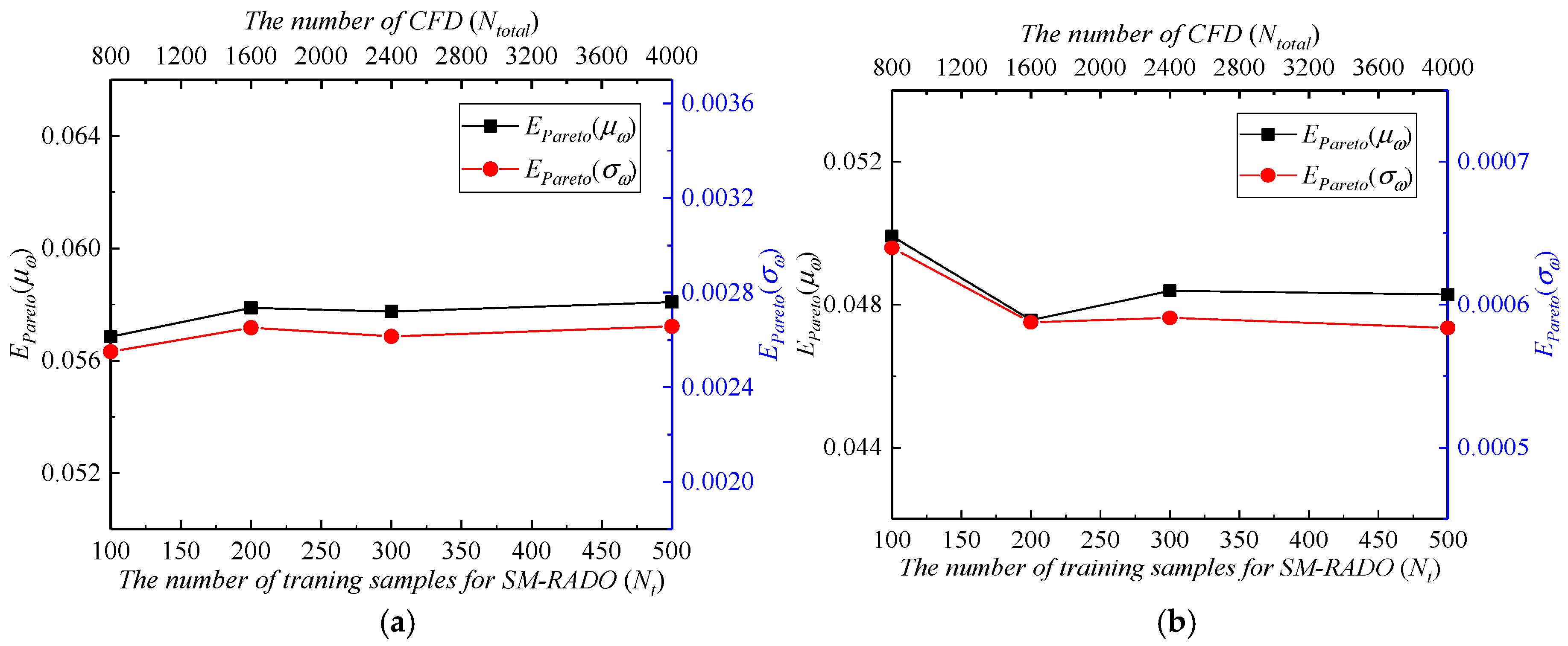
 Figure 15 and Figure 16 depict the variations of SM-RADO results with the number of training samples Nt.
As shown in Figure 15, the relative error εmodel decreases with increasing Nt. When Nt = 500, the εmodel for SM-RADO is approximately 0.69%. However, as shown in Figure 13, the εmodel achieved by the developed ARADO method is only 0.25%, which is lower than that obtained by SM-RADO. This further underscores the precision of the stochastic surrogate model constructed by ARADO in the vicinity of the Pareto optimal solutions.
In Figure 16, after Nt ≥ 300, EPareto(μω) and EPareto(σω) exhibit minimal changes, indicating a convergence towards the overall level of Pareto-optimal solutions. At Nt = 300, EPareto(μω) and EPareto(σω) are 0.057752 and 0.002616, respectively, for α = −8°, and 0.048388 and 0.000591, respectively, for α = 9°, with a total of 2400 CFD evaluations performed for the robust optimization. When Nt = 500, EPareto(μω) and EPareto(σω) are 0.058088 and 0.002658 for α = −8°, and 0.048283 and 0.000584 for α = 9°, requiring 4000 CFD evaluations for the entire robust optimization.
Table 4 compares the EPareto(μω) and EPareto(σω) values obtained by the SM-RADO and ARADO approaches. For SM-RADO with Nt = 100, EPareto(μω) and EPareto(σω) at α = −8° are slightly lower than that for ARADO, but significantly higher at α = 9°. However, for SM-RADO with Nt = 200, 300, and 500, EPareto(μω) and EPareto(σω) are notably higher than that for ARADO, at both α = −8° and 9°. Consequently, the overall level of the Pareto-optimal solutions obtained by ARADO is significantly superior to that obtained by SM-RADO.
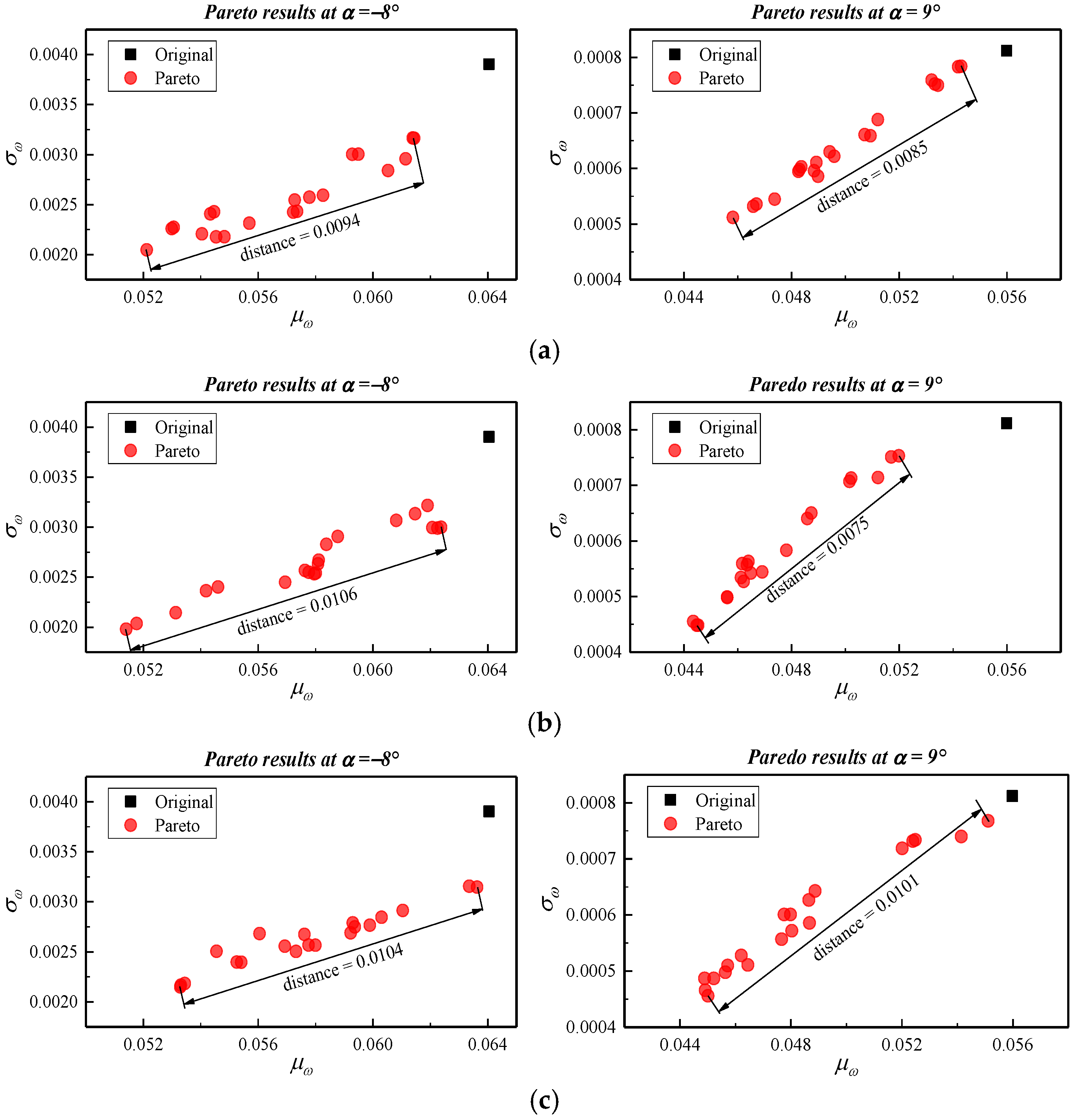
Figure 17 compares the distribution of the Pareto-optimal solutions obtained by M-RADO and ARADO. The optimal solutions obtained by ARADO not only deviate further from the global aerodynamic losses of the original airfoil shape, but are also more concentrated. This suggests that ARADO is more effective in balancing competing optimization objectives, leading to optimization results that are more closely centered around the mean level. From Table 4 and Figure 17, it is clear that the quality of the optimization results achieved by ARADO are notably superior to that of SM-RADO.
Table 4 also presents a comparison of the computational efficiency between SM-RADO and ARADO. It is evident that only the SM-RODO with Nt = 100 requires fewer CFD calculations than ARADO. However, it derived from Table 4 and Figure 17 that the optimization quality of ARADO is significantly superior to that of M-RADO. Therefore, the ARADO method developed can achieve better robust optimization results more quickly.

5.2. Discussion of Optimization Results
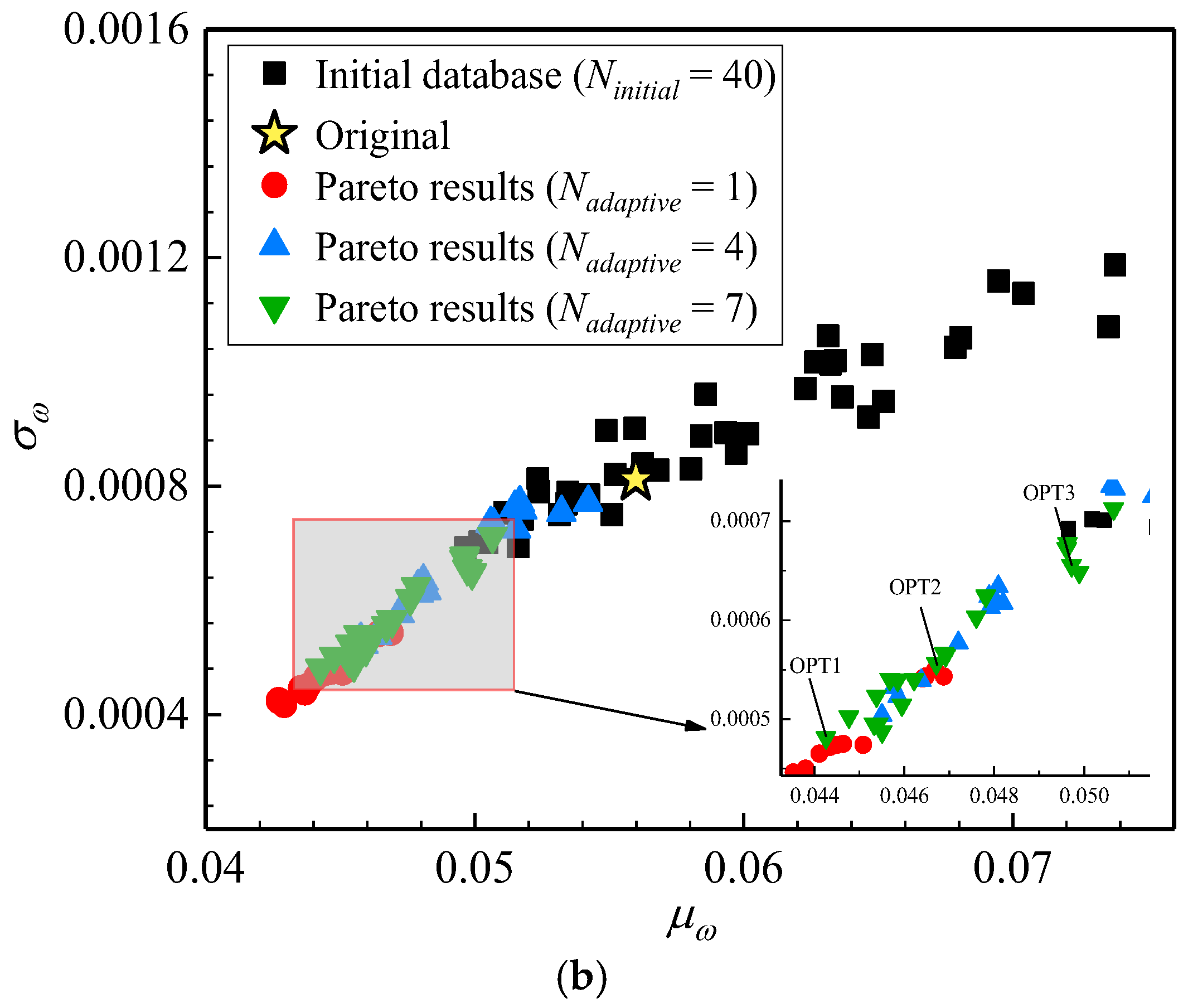
As indicated in Figure 13 and Figure 14, the optimization converged after seven adaptive external iterations. Figure 18 illustrates the variations of the Pareto-optimal solutions with Nadaptive. As ARADO converges, the Pareto set ultimately demonstrates improved robustness in ω for both α = −8° and 9°. To further discuss the final optimization results, three representative optimized airfoils were selected for aerodynamic robustness analysis, denoted as OPT1, OPT2, and OPT3 in Figure 18. 
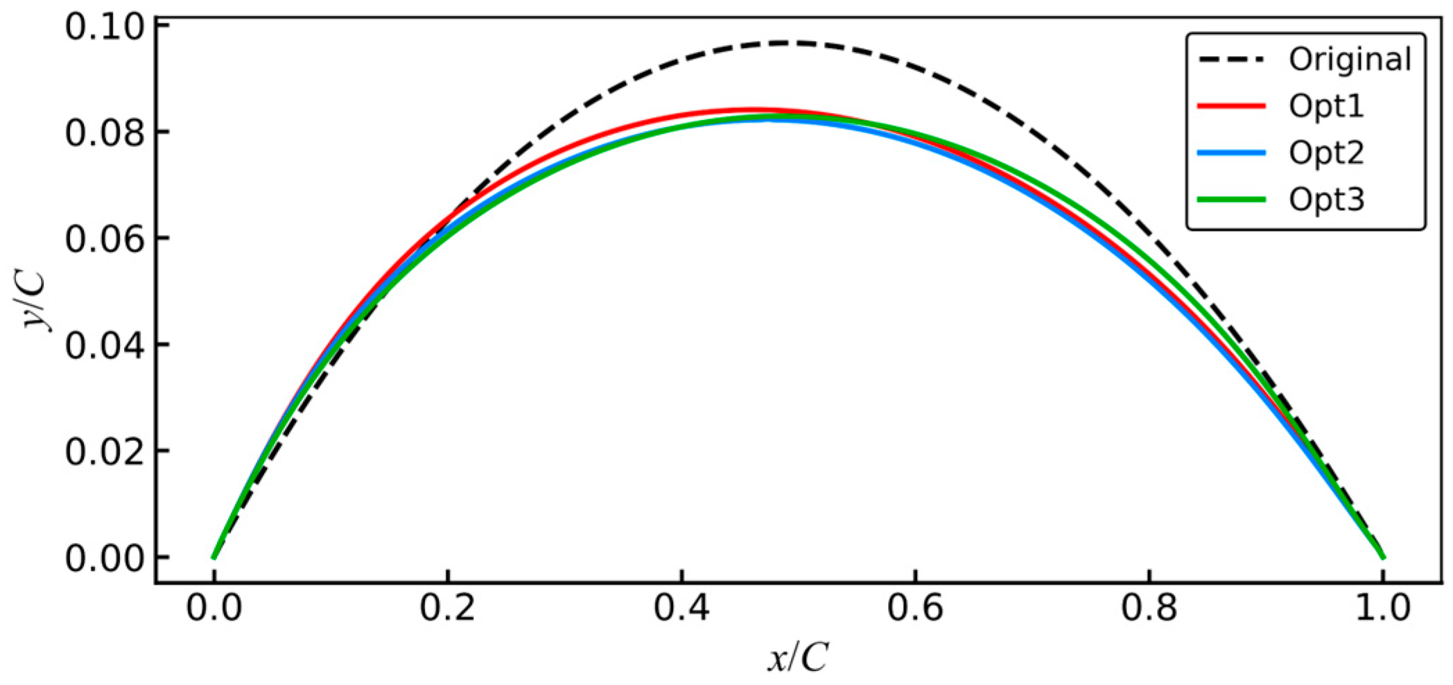
Figure 19 displays the geometric shapes of the original and three optimized airfoils.
Table 5 showcases the values of μω and σω for the original airfoil and three optimized airfoils at α = −8°. When compared to the original design, OPT1, OPT2, and OPT3 demonstrate reductions in μω of 4.40%, 12.18%, and 16.57%, respectively. Additionally, the standard deviations σω for the three optimized airfoils decrease by 22.56%, 37.69%, and 44.10%. Table 6 presents their μω and σω at α = 9°. Relative to the original design, the μω values for the three optimized airfoils decrease by 20.95%, 16.57%, and 11.20%, while the corresponding reductions in σω are 40.76%, 31.53%, and 19.34%, respectively.
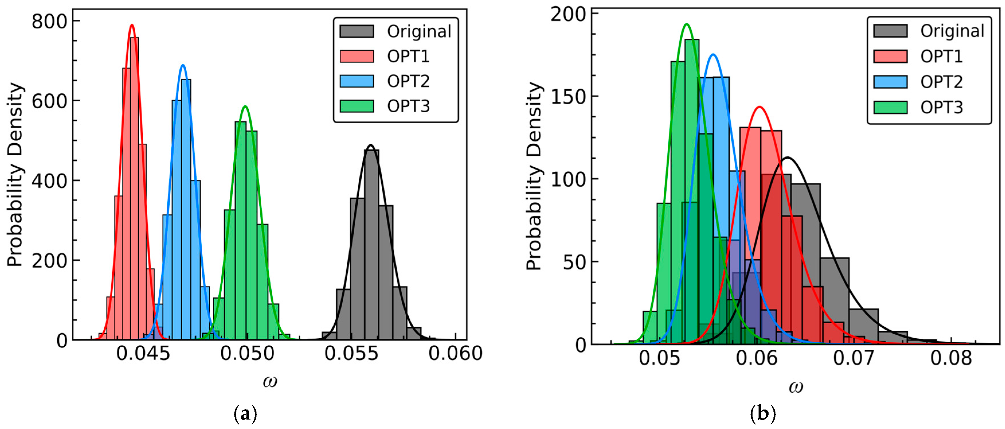
The probability density function (PDF) is a crucial metric for assessing the robustness of aerodynamic performance. Figure 20 illustrates the PDF of ω for both the original and optimized blades. The original design exhibits the widest distribution, indicating a higher level of uncertainty or dispersion in ω. In contrast, the distributions of the three optimized blades are narrower and more peaked, with an overall shift towards lower values. It suggests that under stochastic perturbations in the inflow Ma, the optimized blades demonstrate reduced variability in ω while also achieving a decrease in average aerodynamic loss. A comparison of the PDFs for the three optimized blades reveals the following trends: at α = −8°, the mean levels and dispersions for OPT1, OPT2, and OPT3 decrease successively. Conversely, at α = 9°, those levels for OPT1, OPT2, and OPT3 increase progressively.
By the analysis of Table 5 and Table 6, as well as Figure 20, it can be deduced that the optimized compressor airfoils obtained by the proposed ARADO significantly enhance the robustness of aerodynamic losses at α = −8° and α = 9°. At α = −8°, the incremental improvements in aerodynamic loss robustness for OPT1, OPT2, and OPT3 decrease successively. Similarly, at α = 9°, the enhancements in the robustness for OPT1, OPT2, and OPT3 decrease successively.
To confirm that the optimized blades also enhance the robustness of the diffusion capability, Table 7 provides μ C p and σ C p at α = −8° for the original and three optimized blades. Compared to the original, OPT1, OPT2, and OPT3 show respective increases of 3.96%, 9.02%, and 12.55% in μ C p , along with decreases of 36.36%, 64.98%, and 76.90% in σ C p . Table 8 presents the statistical moments at α = 9°. In comparison to the original, μ C p for the three optimized blades increased by 2.96%, 2.14%, and 1.44% respectively, while the σ C p increased by 18.38%, 13.86%, and 8.27% respectively.
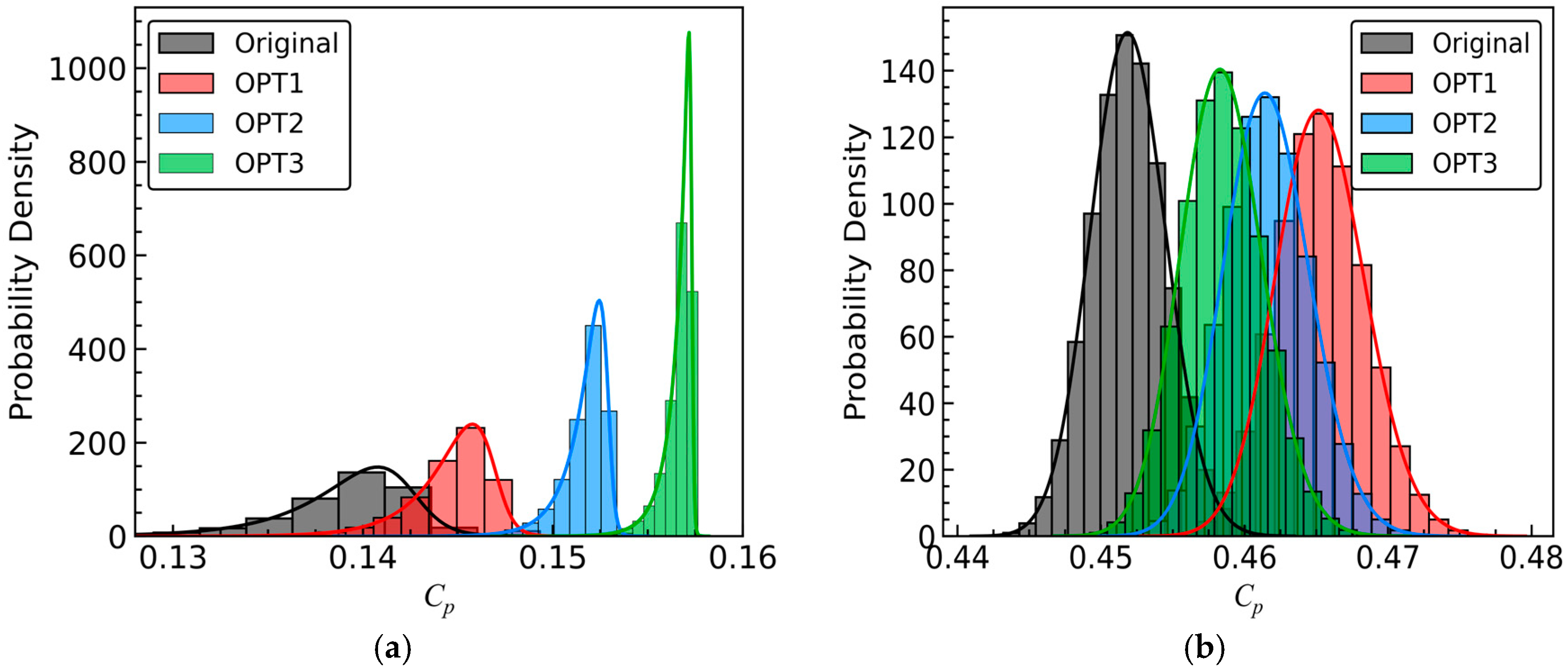
Figure 21 illustrates the PDFs of Cp for both the original and optimized blades. It indicates that at α = −8°, the optimized blades exhibit reduced variability in diffusion capability and an increase in average diffusion capability. Comparing the PDFs of the three optimized stator blades reveals that the average levels of diffusion capability for OPT1, OPT2, and OPT3 increase successively, while their dispersions decrease successively.
At α = 9°, in contrast to the original, the distributions of the optimized blades shift towards higher values, albeit slightly wider and shorter. This suggests an increase in the average diffusion capability, accompanied by a slight increase in the dispersion of diffusion capability. Nonetheless, the probability that their Cp exceeds the original is over 60%, as depicted in Figure 21b. Therefore, it is still reasonable to assert that the three optimized stator blades enhance the robustness of diffusion capability at α = 9°. Comparing the PDFs of the three optimized blades reveals that the average levels for OPT1, OPT2, and OPT3 decrease successively, while the probabilities that Cp exceeds the original decrease successively.
Through the analysis of Table 7 and Table 8, and Figure 21, it can be concluded that the optimized blades can enhance the robustness of diffusion capability at both α = −8° and α = 9°. At α = −8°, the incremental improvements in the robustness of diffusion capability for OPT1, OPT2, and OPT3 increase successively. Conversely, at α = 9°, the enhancements in the robustness of diffusion capability decrease successively.
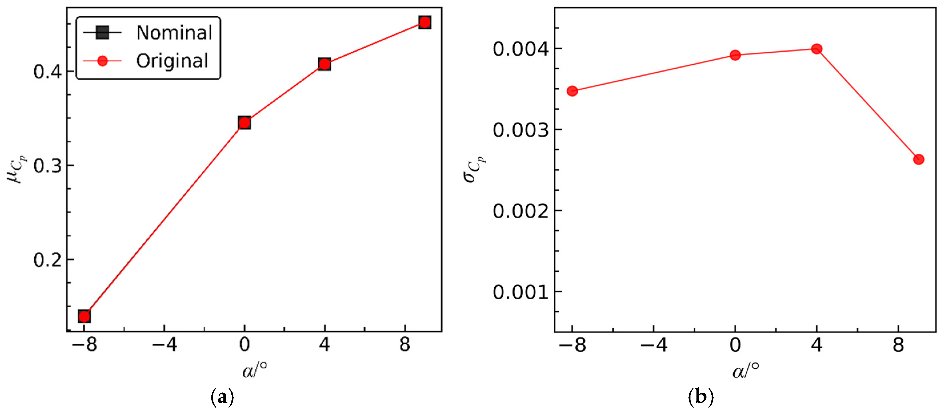
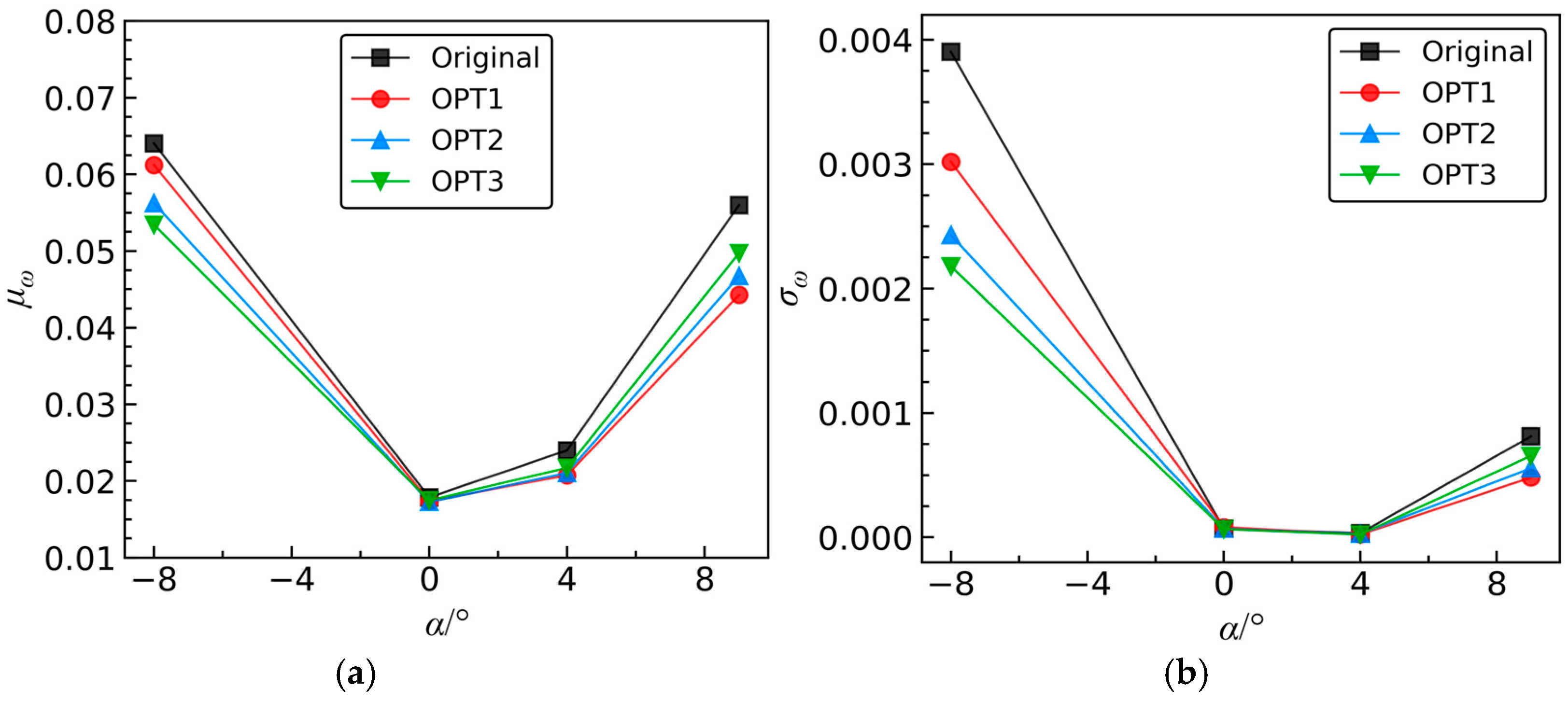
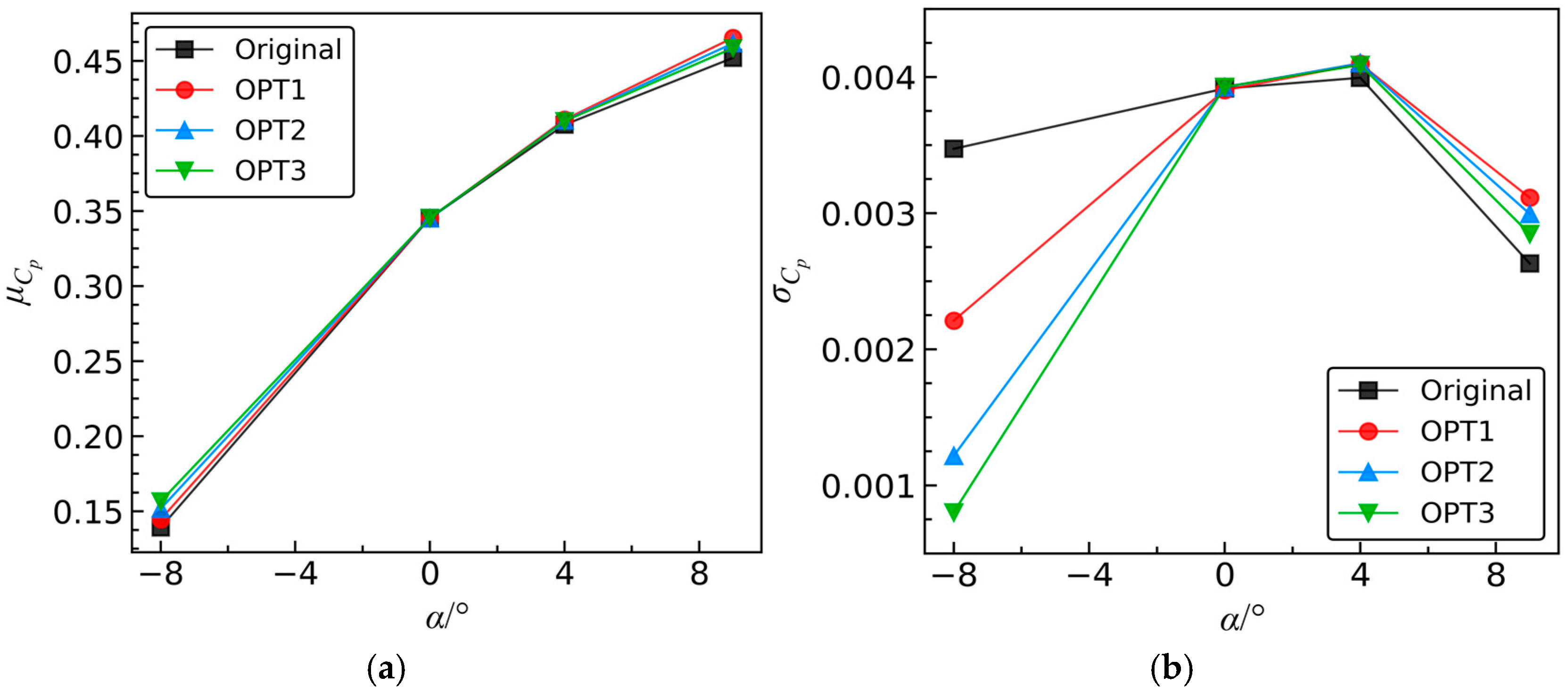
Figure 22 presents the variations of μω and σω for the original and optimized blades with the increase in incidence α, while Figure 23 illustrates the variations of μ C p and σ C p . At α = 0° and α = 4°, the statistical moments of the aerodynamic coefficients exhibit minimal differences compared to the original values. This indicates that the improvement in aerodynamic performance robustness near the design operating incidence is limited. This phenomenon arises because the flow is relatively stable when operating near the design conditions [30,44], resulting in less impact from stochastic fluctuations in the inflow Ma. Therefore, near the operating incidence, the aerodynamic robustness of the optimized blades remains at a consistently good level similar to the original blade. In other words, the optimized results can enhance the robustness of aerodynamic performance across all operating incidences.
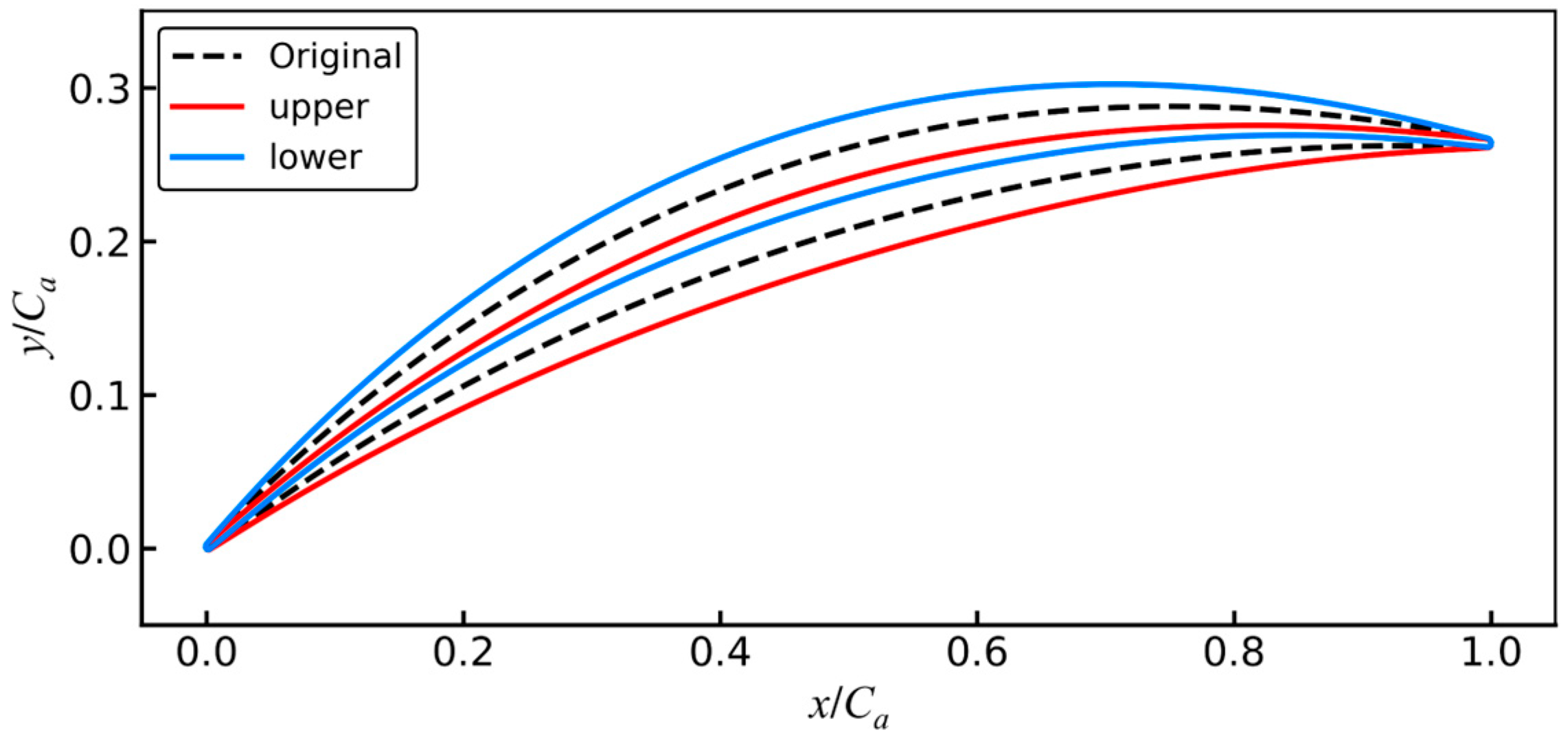
Aerodynamic robustness optimization results can serve as a reference for aerodynamic designers of compressors. The primary design variable changes involve modifications to the camber line. Hence, a comparative analysis of the camber lines was conducted, and the results are depicted in Figure 24. After optimization, the leading edge angle increases, the position of maximum curvature shifts forward along the chord, the maximum curvature decreases, and the trailing edge angle decreases.
Table 9 further provides the leading edge angle, maximum curvature position, maximum curvature, and trailing edge angle of the three optimized blades. The results indicate that OPT1, OPT2, and OPT3 sequentially increase the leading edge angle, and the maximum curvature position moves backward along the chord length in sequence. In addition, the maximum curvature, as well as the trailing edge angle, first decreases and then increases for OPT1, OPT2, and OPT3.

5.3. Analysis of Flow Field

In the context of OPT1, OPT2, and OPT3, OPT2 stands out as a compromise solution that enhances aerodynamic robustness at both α = −8° and α = 9°. Therefore, OPT2 is focused on as a case study to elucidate the flow mechanisms that optimization solutions improve aerodynamic robustness.
Initially, the mechanism for improving aerodynamic robustness at α = −8° is examined. 
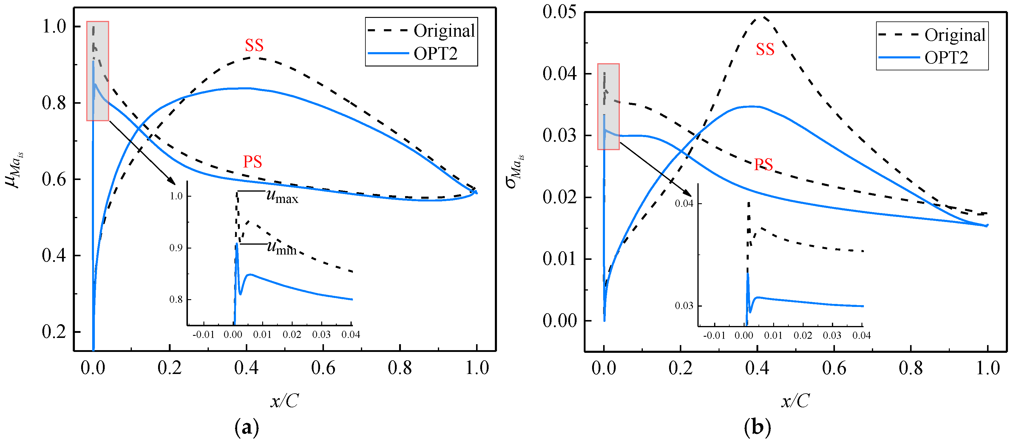
Figure 25 illustrates the distribution of μ M a i s and σ M a i s on the blade surface. 
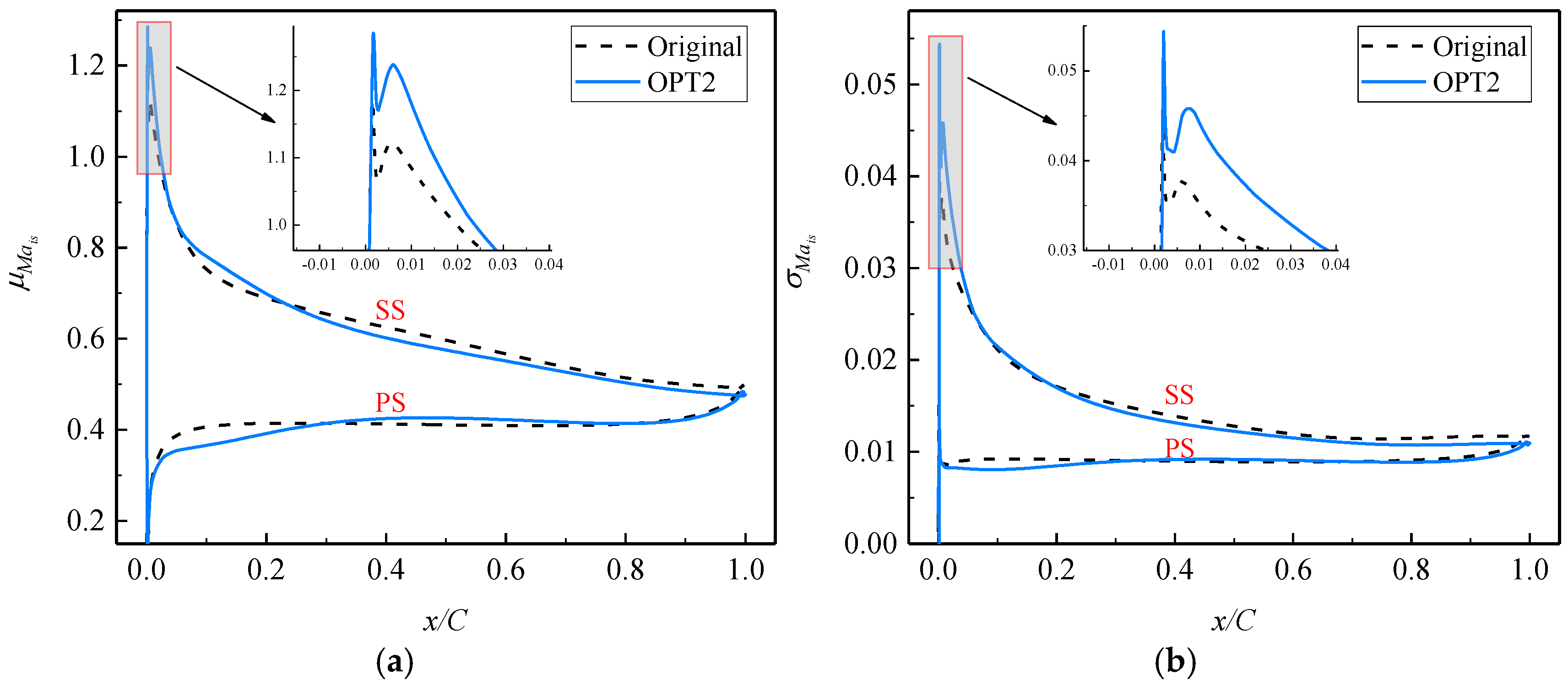
Figure 25a reveals significant alterations in the average flow near the velocity spike on the pressure side (PS) after robustness optimizations. The spike diffusion factor Dspike provides a quantification of the spike strength [49]:
D s p i k e = 1 u min u max
where umax and umin are the velocities at the peak and subsequent trough on the spike, as in Figure 25a. When Dspike ≥ 0.10, the leading edge separation bubble occurs. A larger Dspike corresponds to a more pronounced leading edge separation. The mean Dspike on the PS of the original is approximately 0.1064, while that of OPT2 is around 0.1082. Hence, for OPT2, the average size of the leading edge separation bubble on the PS is expected to increase.
The results from Figure 25a also indicate that after aerodynamic robustness optimizations, the average aerodynamic load on the suction side (SS) and PS notably decreases. This suggests that compared to the original, the boundary layer thickness on the SS and PS decreases. 
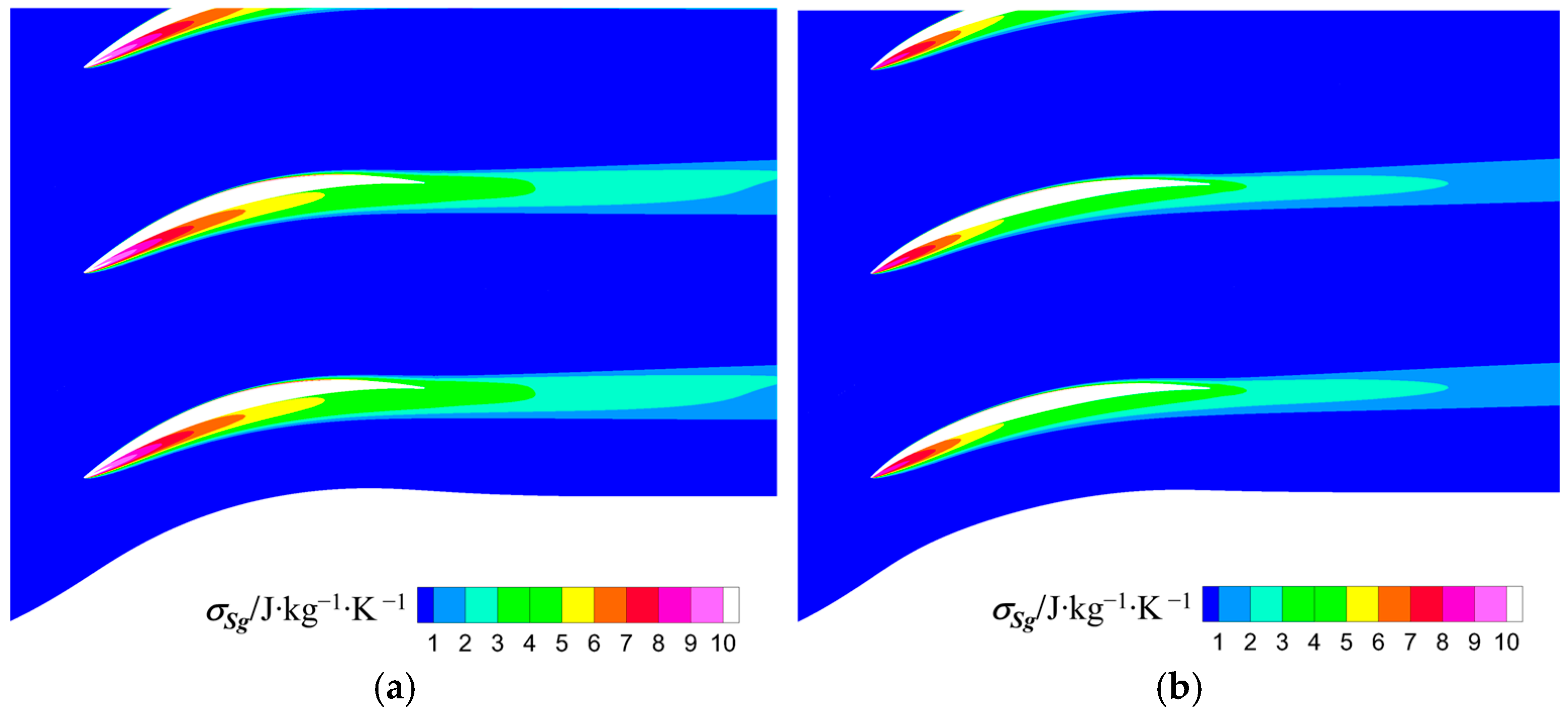
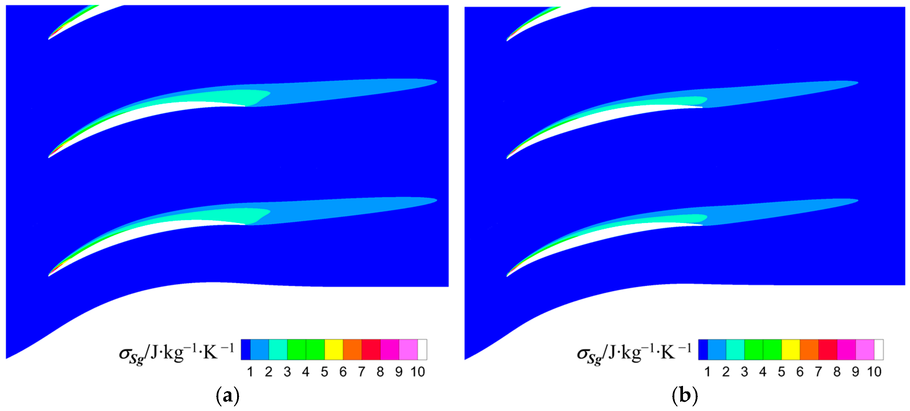
Figure 26 compares the μ M a i s distribution inside the blade passage between the original and OPT2. While OPT2 exacerbates separation flow at the leading edge of PS, its improvement in the boundary layer flow on the SS and PS is more pronounced. Therefore, OPT2 reduces the average global aerodynamic losses relative to the original and enhances the average diffusion capability in the airflow.
The σ M a i s distribution on the blade surface shown in Figure 25b indicates that after robustness optimizations, the fluctuation amplitude of the velocity spikes at the leading edge of PS, as well as the aerodynamic load fluctuations on the SS and PS decreases. Consequently, for OPT2, the fluctuations in the leading edge separation and boundary layer losses decreases, leading to a reduction in the fluctuations of the global aerodynamic losses, as illustrated by the distribution of the standard deviation of entropy generation ( σ S g ), shown in Figure 27.
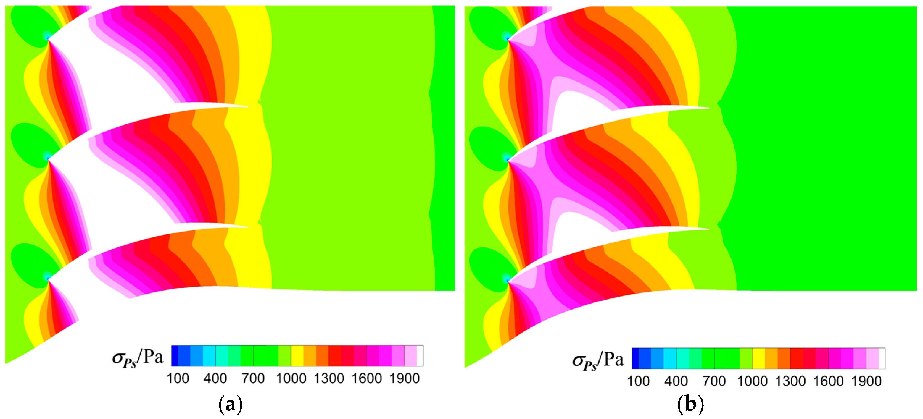
Figure 28 contrasts the standard deviations of static pressure, σPs, inside the passage between the original and OPT2. Combining Figure 28 with Figure 25b, it can be inferred that due to the reduced fluctuation amplitude of the velocity spike at the leading edge of PS, and the significant reduction in aerodynamic load fluctuations on the SS, the fluctuations in the loading of the leading edge and SS decrease. As a consequence, for OPT2, the random disturbances of the diffusion capability are reduced.
Then, the mechanism of improving aerodynamic robustness at α = 9° was analyzed. Figure 28 shows the distribution of μ M a i s and σ M a i s on the blade surface. In Figure 29a, it is evident that following robustness optimizations, there is a substantial improvement in the average flow near the velocity spike on the SS. Through the calculation outlined in Equation (20), the mean Dspike on the SS for the original is approximately 0.1020, whereas for OPT2, it is around 0.1001. As a result, OPT will decrease the average size of the leading edge separation bubble on the SS, compared to the original.
Research findings from references [2,44] suggest that the size of the leading edge separation bubble will impact the development of the downstream boundary layer. Figure 30 provides the μ M a i s distribution and average streamlines inside the passages for the original and OPT2. For OPT2, due to the reduction in the leading edge separation bubble on the SS, the thickness of the downstream boundary layer decreases, and the separation scale near the trailing edge of SS diminishes. Consequently, OPT2 lowers the average level of global aerodynamic losses and enhances its average ability to diffuse airflow.
Figure 29b shows that, although the fluctuation amplitude of the velocity spike at the leading edge of SS is increased for OPT2, the fluctuation amplitude of flows on the SS after the 20% chord decreases. Figure 31 compares the distribution of σ S g between the original and OPT2. For OPT2, the reduction in fluctuations caused by the boundary layer thickness over the SS leads to a decrease in the fluctuations of global aerodynamic losses. Hence, the reduction in fluctuations of the global losses for OPT2 is primarily due to the suppression of uncertainties in the flow on the SS after the 20% chord.
Figure 32 compares the distribution of σPs inside the passage between the original and OPT2. Combining this with the analysis of Figure 29b, it can be deduced that due to the increased aerodynamic load fluctuations at the leading edge of SS, the load variation on the front part of OPT2 is more pronounced, leading to an increase in random disturbances in the airflow diffusion process. Nonetheless, analysis from Figure 21b indicates that the probability of the optimized blade’s Cp being higher than that of the original is over 60%. Therefore, it can still be argued that OPT2 enhances the robustness of the blade’s diffusion capability at α = 9°.

6. Conclusions

Traditional M-RADO relies on a global surrogate model, where the optimization outcome is contingent upon the approximation accuracy of the surrogate model, typically necessitating a substantial number of training samples to ensure its precision. To mitigate the computational burden of M-RADO, the study introduces a novel adaptive strategy, combining advanced NGPR surrogate techniques with the NSGA-III algorithm to propose a multi-objective ARADO methodology. Employing the introduced novel sparse PCE, namely OMP-based sparse PCE, to construct the stochastic NGPR surrogate model encompassing statistical features of aerodynamic characteristics significantly enhances the efficiency of acquiring each training sample for NGPR. The adaptive strategy mandates the NGPR model to achieve precision only in the vicinity of the optimal solutions, rather than demanding high accuracy across the entire design space. Throughout the optimization process, the model undergoes adaptive updates based on the historical optimization results, markedly reducing the experimental points required for training the model while achieving robust optimization effects.
Considering the typical uncertainty fluctuation source at the compressor inlet, Mach number, the developed ARADO is applied to the robust aerodynamic design optimization of a high subsonic compressor airfoil across all operating incidences. Initially, from the results of aerodynamic uncertainty analysis, it is evident that the OMP-based sparse PCE method, due to the incorporation of advanced sparse signal processing concepts, significantly outperforms DMC in terms of analysis efficiency and enhances the efficiency by nearly half compared to full PCE. Subsequently, from the robust optimization results, it is observed that with fewer training samples, the proposed ARADO attains Pareto-optimal solution sets with a significantly superior average level compared to M-RADO. Simultaneously, the ARADO method better balances various optimization objectives, concentrating the space distribution of Pareto-optimal solutions closer to the average level. Therefore, the developed ARADO effectively attains higher-quality robust aerodynamic design optimization results.
As the adaptive robust optimization converges, the Pareto-optimal solution set ultimately manages to enhance aerodynamic robustness at off-design incidences. Near the design incidences, the aerodynamic robustness of the optimization results remains consistently at a good level akin to the original. Among the three typical optimized blades selected from the Pareto-optimal solutions, denoted as OPT1, OPT2, and OPT3, the leading edge angle of them increases, the maximum deflection position shifts forward along the chord, and both the maximum deflection and trailing edge angle decrease, compared to the original. This conclusion can guide compressor blade designers in creating aerodynamically more robust blade profiles. At a high negative operating incidence, μω for OPT1, OPT2, and OPT3 decrease by 4.40%, 12.18%, and 16.57% relative to the original, with their corresponding σω decreasing by 22.56%, 37.69%, and 44.10%. Conversely, at a high positive incidence, their μω decreases by 20.95%, 16.57%, and 11.20%, while their σω decreases by 40.76%, 31.53%, and 19.34%. Moreover, the ARADO’ results enhance μ C p while controlling σ C p diversity, thus aligning more closely with practical engineering requirements.

Author Contributions

Conceptualization, Z.G. and L.B.; methodology, Z.G. and L.B.; software, W.C.; validation, Z.G., L.B. and C.L.; formal analysis, Z.G. and C.L.; investigation, Z.G. and C.L.; resources, X.G. and W.C.; data curation, Z.G. and L.B.; writing—original draft preparation, Z.G. and L.B.; writing—review and editing, X.G. and W.C.; visualization, C.L.; supervision, X.G. and W.C.; project administration, X.G. and W.C.; funding acquisition, Z.G., C.L. and W.C. All authors have read and agreed to the published version of the manuscript.

Funding

This research was funded by Technology Innovation Talent Project of National University of Defense Technology, National University of Defense Technology Independent Innovation Scientific Fund (Grant No. ZK24-62), and National Major Science and Technology Project of China (Grant No. J2019-I-0011-0011).

Data Availability Statement

Data are contained within the article.

Conflicts of Interest

The authors declare that they have no known competing financial interests or personal relationships that could have appeared to influence the work reported in this paper.

Nomenclature

Symbols
a ^ PCE coefficients
CChord
CaAxial chord
CpStatic pressure coefficient
dDimension of uncertain variables
DspikeDiffusion factor of velocity spikes
HPCE basis functions
hVertical distance between control points and chord
MaMach number
MaisIsentropic Mach number
NNumber of samples to construct PCE
NadptiveNumber of samples in Pareto set at current external iteration
NinitialNumber of aerodynamic shape samples used to train initial NGPR
NtAerodynamic shape training database in SM-RADO
NtotalTotal number of CFD simulations required for robust optimization
NupdatedNumber of updates for NGPR model
NUQTotal number of CFD simulations invoked for UQ
pPolynomial order of PCE
PNumber of terms in full PCE
PsStatic pressure
PtTotal pressure
qAerodynamic performance metric
SgEntropy generation
αOperating incidence
βBasis function vector in GPR or NGPR
ε(EPareto(fi))Relative error of the means of an objective fi in Pareto set
ε0Convergence threshold of ARADO
εmodelRelative error between surrogate model and CFD
θCoefficient vector in GPR or NGPR
μqMean value of variable q
ξUncertain variables
σqStandard deviation of variable q
ωGlobal total pressure loss coefficient
Acronyms
CFDComputational fluid dynamics
DADODeterministic aerodynamic design optimization
DMCDirect Monte Carlo
GPRGaussian process regression
G-RADOGradient-based RADO
NGPRNoisy Gaussian process regression
NSGANon-dominated sorting genetic algorithm
OMPOrthogonal matching pursuit
PCEPolynomial chaos expansion
PDFProbability density function
PSPressure side
RADORobust aerodynamic design optimization
RBFRadial basis function
SM-RADOSurrogate model-based RADO
SSSuction side
SSMStochastic surrogate model
TETrailing edge
UQUncertainty quantification

Appendix A. Benefits of NGPR

To validate the benefits of the NGPR modeling approach, a function experiment is presented. The function is
f x = sin 0.15 x + 0.05 e x 30 , x 0 , 150
Figure A1 resents the function curve of the test function. In the function space, 50 samples are used as the training set, as shown in Figure A1a. Subsequently, the random noise perturbations are applied to each training sample, as depicted in Figure A1b. Based on the noisy training sample set, Figure A2 compares the effectiveness of GPR and NGPR in approximating the test function. The curve approximated by NGPR aligns more closely with the function, while the GPR exhibits significant distortion. Therefore, the NGPR method is more effective for regression problems in aerodynamic responses influenced by numerical fluctuations in CFD.

Appendix B. Benefits of NSGA-III

To validate the superiority of the introduced NSGA-III, the classic test function DTLZ1 [50] is selected to test both the NSGA-II and NSGA-III. The optimization problem description of the ZDLZ1 test function is
Find :                           x 12 Min :                           f 1 x = 1 2 x 1 x 2 1 + g x f 2 x = 1 2 x 1 1 x 2 1 + g x f 3 x = 1 2 1 x 1 1 + g x                                                   where   g x = 100 10 + i = 3 12 x i 0.5 2 cos 20 π x i 0.5 Subject   to :         0 x i 1 ,   i = 1 , 2 , , 12
When optimizing the ZDLR1, set a population size of 100, 500 evolutionary iterations, a crossover rate of 0.9, and a mutation rate of 0.1. Figure A3 compares the Pareto solutions. NSGA-III tends to favor individuals excelling across all three objectives, while NSGA-II tends to produce individuals with a bias towards a single objective. It confirms that when dealing with RADO with more than two objectives, NSGA-III’s Pareto solutions are more comprehensive, aiding in optimal solution selection.

References

  1. Garzon, V.E.; Darmofal, D.L. Impact of geometric variability on axial compressor performance. J. Turbomach. 2003, 125, 1199–1213. [Google Scholar] [CrossRef]
  2. Guo, Z.; Chu, W.; Zhang, H. Novel data-driven sparse polynomial chaos and analysis of covariance for aerodynamics of compressor cascades with dependent geometric uncertainties. Chin. J. Aeronaut. 2024, 37, 89–108. [Google Scholar] [CrossRef]
  3. Li, J.; Du, J.; Liu, Y.; Zhang, H.; Nie, C. Effect of inlet radial distribution on aero-dynamic stability in a multi-stage axial flow compressor. Aerosp. Sci. Technol. 2020, 105, 105886. [Google Scholar] [CrossRef]
  4. Seshadri, P.; Shahpar, S.; Parks, G. Aggressive Design in Turbomachinery. In Proceedings of the 16th AIAA Non-Deterministic Approaches Conference, No. AIAA 2014-1007, National Harbor, MD, USA, 13–17 January 2014. [Google Scholar]
  5. Fentaye, A.D.; Baheta, A.T.; Gilani, S.I.; Kyprianidis, K.G. A review on gas turbine gas-path diagnostics: State-of the-art methods, challenges and opportunities. Aerospace 2019, 6, 83. [Google Scholar] [CrossRef]
  6. Papadimitriou, D.; Papadimitriou, C. Aerodynamic shape optimization for minimum robust drag and lift reliability constraint. Aerosp. Sci. Technol. 2016, 55, 24–33. [Google Scholar] [CrossRef]
  7. Du, X.; Leifsson, L. Optimum aerodynamic shape design under uncertainty by utility theory and metamodeling. Aerosp. Sci. Technol. 2019, 95, 105464. [Google Scholar] [CrossRef]
  8. Fusi, F.; Congedo, P.; Guardone, A.; Quaranta, G. Assessment of robust optimization for design of rotorcraft airfoils in forward flight. Aerosp. Sci. Technol. 2020, 107, 106355. [Google Scholar] [CrossRef]
  9. Lange, A.; Voigt, M.; Vogeler, K.; Schrapp, H.; Johann, E.; Guemmer, V. Impact of Manufacturing Variability on Multistage High-Pressure Compressor Performance. J. Eng. Gas Turb. Power 2012, 134, 417–426. [Google Scholar] [CrossRef]
  10. Schnell, R.; Lengyel-Kampmann, T.; Nicke, E. On the impact of geometric variability on fan aerodynamic performance, unsteady blade row interaction, and its mechanical characteristics. J. Turbomach. 2014, 136, 091005. [Google Scholar] [CrossRef]
  11. Chen, Z.; Luo, J.; Xia, Z.; Zou, Z.; Du, P.; Liu, F. Statistical investigations of profile error impact on flow and performance of a low-pressure turbine cascade. Phys. Fluids 2023, 35, 126114. [Google Scholar] [CrossRef]
  12. Zhang, Q.; Xu, S.; Yu, X.; Liu, J.; Wang, D.; Huang, X. Nonlinear uncertainty quantification of the impact of geometric variability on compressor performance using an adjoint method. Aerosp. Sci. Technol. 2022, 35, 17–21. [Google Scholar] [CrossRef]
  13. Liu, Y.; Qin, R.; Ju, Y.; Spence, S.; Zhang, C. Impact of realistic manufacturing uncertainties on the aerodynamic performance of a transonic centrifugal impeller. In Proceedings of the ASME Turbo Expo 2020: Turbine Technical Conference and Exposition, No. GT2020-14784, London, UK, 22–26 June 2020. [Google Scholar]
  14. Guo, Z.; Chu, W. A data-driven non-intrusive polynomial chaos for performance impact of high subsonic compressor cascades with stagger angle and profile errors. Aerosp. Sci. Technol. 2022, 129, 107802. [Google Scholar] [CrossRef]
  15. Xia, Z.; Luo, J.; Liu, F. Statistical evaluation of performance impact of flow variations for a transonic compressor rotor blade. Energy 2019, 189, 116285. [Google Scholar] [CrossRef]
  16. Li, Z.; Zheng, X. Review of design optimization methods for turbomachinery aerodynamics. Prog. Aerosp. Sci. 2017, 93, 1–23. [Google Scholar] [CrossRef]
  17. Luo, J.; Xia, Z.; Liu, F. Robust design optimization considering inlet flow angle variations of a turbine cascade. Aerosp. Sci. Technol. 2021, 116, 106893. [Google Scholar] [CrossRef]
  18. Ma, Y.; Du, J.; Yang, T.; Shi, Y.; Wang, L.; Wang, W. Aerodynamic robust design research using adjoint-based optimization under operating uncertainties. Aerospace 2023, 10, 831. [Google Scholar] [CrossRef]
  19. Shi, Y.; Lan, Q.; Lan, X.; Wu, J.; Yang, T.; Wang, B. Robust optimization design of a flying wing using adjoint and uncertainty-based aerodynamic optimization approach. Struct. Multidiscip. Optim. 2023, 66, 110. [Google Scholar] [CrossRef]
  20. Zhang, J.; Li, L.; Dong, X.; Zhang, Z.; Zhang, Y.; Lu, X. A discrete adjoint framework coupled with adaptive PCE for robust aerodynamic optimization of turbomachinery under flow uncertainty. Aerosp. Sci. Technol. 2023, 142, 108592. [Google Scholar] [CrossRef]
  21. Zhao, K.; Gao, Z.; Huang, J. Robust design of natural laminar flow supercritical airfoil by multi-objective evolution method. Appl. Math. Mech. 2014, 35, 191–202. [Google Scholar] [CrossRef]
  22. Fusi, F.; Guardone, A.; Quaranta, G.; Congedo, P.M. Multifidelity physics-based method for robust optimization applied to a hovering rotor airfoil. AIAA J. 2015, 53, 3448–3465. [Google Scholar] [CrossRef]
  23. Wang, X.; Hirsch, C.; Liu, Z.; Kang, S.; Lacor, C. Uncertainty based robust aerodynamic optimization of rotor blades. Int. J. Numer. Meth. Eng. 2013, 94, 111–127. [Google Scholar] [CrossRef]
  24. Gouttiere, A.; Wunsch, D.; Nigro, R.; Barbieux, V.; Hirsch, C. Robust design optimization of an industrial 1.5 stage axial compressor under operational and geometrical uncertainties. In Proceedings of the ASME Turbo Expo 2021: Turbine Technical Conference and Exposition, GT2021-58603, Virtual, 7–11 June 2021. [Google Scholar]
  25. Wang, H.; Gao, L.; Yang, G.; Wu, B. A data-driven robust design optimization method and its application in compressor blade. Phys. Fluids 2023, 35, 066114. [Google Scholar]
  26. Epstein, B.; Peigin, S. Optimization of 3D wings based on Navier-Stokes solutions and genetic algorithms. Int. J. Comput. Fluid D 2006, 20, 75–92. [Google Scholar] [CrossRef]
  27. Khurana, M.S.; Winarto, H.; Sinha, A.K. Application of swarm approach and artificial neural networks for airfoil shape optimization. In Proceedings of the 12th AIAA/ISSMO Multidisciplinary Analysis and Optimization Conference, AIAA Conference Paper, No. AIAA-2008-5954, Victoria, BC, Canada, 10–12 September 2008. [Google Scholar]
  28. Wang, X.; Damodaran, M. Aerodynamic shape optimization using computational fluid dynamics and parallel simulated annealing algorithms. AIAA J. 2001, 39, 1500–1508. [Google Scholar] [CrossRef]
  29. Loeven, G.J.A.; Witteveen, J.A.S.; Bijl, H. The application of the probabilistic collocation method to a transonic axial flow compressor. In Proceedings of the AIAA/ASME/ASCE/AHS/ASC Structures, Structural Dynamics, and Materials Conference, AIAA 2010-2923, Orlando, FL, USA, 12–15 April 2010. [Google Scholar]
  30. Guo, Z.; Chu, W.; Zhang, H. Effects of inlet incidence perturbations on compressor cascade performance using adaptive sparse grid collocation. J. Appl. Fluid Mech. 2023, 16, 1281–1295. [Google Scholar]
  31. Ju, Y.; Zhang, C. Robust design optimization method for centrifugal impellers under surface roughness uncertainties due to blade fouling. Chin. J. Mech. Eng. 2016, 29, 301–314. [Google Scholar] [CrossRef]
  32. Cheng, H.; Li, Z.; Duan, P.; Lu, X.; Zhao, S.; Zhang, Y. Robust optimization and uncertainty quantification of a micro axial compressor for unmanned aerial vehicles. Appl. Energe 2023, 352, 121972. [Google Scholar] [CrossRef]
  33. Ma, C.; Gao, L.; Cai, Y.; Li, R. Robust optimization design of compressor blade considering machining error. In Proceedings of the ASME Turbo Expo 2017: Turbine Technical Conference and Exposition, GT2017-63157, Charlotte, NC, USA, 26–30 June 2017. [Google Scholar]
  34. Song, Z.; Zheng, X.; Wang, B.; Zhou, K.; Adjei, R.A. Multidisciplinary robust optimization approach of fan rotors under structural constraints with blade curvature. Aerosp. Sci. Technol. 2023, 142, 108637. [Google Scholar] [CrossRef]
  35. Li, Q.; Chu, W.; Dong, J.; Ji, T. Data Mining-Based optimization study on T-shaped multiple groove casing treatment for axial compressor stability. Phys. Fluids 2024, 36, 116132. [Google Scholar] [CrossRef]
  36. Chi, Z.; Chu, W.; Zhang, H.; Zhang, Z. Stall margin evaluation and data mining based multi-objective optimization design of casing treatment for an axial compressor rotor. Phys. Fluids 2023, 35, 086117. [Google Scholar] [CrossRef]
  37. Rasmussen, C.E.; Williams, C.K.I. Gaussian Processes in Machine Learning; MIT Press: Cambridge, MA, USA, 2006. [Google Scholar]
  38. Deb, K.; Jain, H. An evolutionary many objective optimization algorithm using reference point based nondominated sorting approach, Part I: Solving problems with box Constraints. IEEE Trans. Evol. Comput. 2014, 18, 577601. [Google Scholar] [CrossRef]
  39. Xiu, D.; Karniadakis, G. The Wiener-Askey polynomial chaos for stochastic differential equations. SIAM J. Sci. Comput. 2002, 24, 619–644. [Google Scholar] [CrossRef]
  40. Guo, Z.; Chu, W.; Zhang, H.; Liu, K. An efficient sparse surrogate model for supersonic aerodynamics of a compressor cascade with uncertain geometric deformations. Aerosp. Sci. Technol. 2024, 150, 109133. [Google Scholar] [CrossRef]
  41. Hosder, S.; Walters, R.W.; Balch, M. Efficient sampling for non-intrusive polynomial chaos applications with multiple uncertain input variables. In Proceedings of the 48th Structures, Structural Dynamics, and Materials Conference, No. AIAA2007-1939, Honolulu, HI, USA, 23–26 April 2007. [Google Scholar]
  42. Maitre, O.P.L.; Knio, O.M. Spectral Methods for Uncertainty Quantification: With Applications to Computational Fluid Dynamics; Springer Science and Business Media: Berlin, Germany, 2010. [Google Scholar]
  43. Blatman, G.; Sudret, B. Sparse polynomial chaos expansion based on least angle regression. J. Comput. Phys. 2011, 230, 2345–2367. [Google Scholar] [CrossRef]
  44. Guo, Z.; Chu, W.; Zhang, H.; Liang, C.; Meng, D. Aerodynamic evaluation of cascade flow with actual geometric uncertainties using an adaptive sparse arbitrary polynomial chaos. Phys. Fluids 2023, 35, 036122. [Google Scholar] [CrossRef]
  45. Thapa, M.; Mulani, B.S.; Walters, W.R. Adaptive weighted least-squares polynomial chaos expansion with basis adaptivity and sequential adaptive sampling. Comput. Methods Appl. Mech. Eng. 2020, 360, 112759. [Google Scholar] [CrossRef]
  46. Mallat, S.; Zhang, Z. Matching pursuits with time-frequency dictionaries. IEEE Trans. Signal Process 1993, 41, 3397–3415. [Google Scholar] [CrossRef]
  47. Li, X.; Lu, Q.; You, F.; Cui, Y.; Zhu, Z. Qualitative influence of blade machining deviation on cascade critical angle of attack. J. Aerosp. Power 2024, 39, 440–453. [Google Scholar]
  48. Wu, X.; Zhang, W.; Song, S.; Ye, Z. Sparse grid-based polynomial chaos expansion for aerodynamics of an airfoil with uncertainties. Chin. J. Aeronaut. 2018, 31, 997–1011. [Google Scholar] [CrossRef]
  49. Goodhand, M.N.; Miller, R.J. Compressor leading edge spikes: A new performance criterion. J. Turbomach. 2011, 33, 021006. [Google Scholar] [CrossRef]
  50. Deb, K.; Thiele, L.; Laumanns, M.; Zitzler, E. Scalable multi-objective optimization test problems. In Proceedings of the 2002 Congress on Evolutionary Computation. CEC’02 (Cat. No.02TH8600), Honolulu, HI, USA, 12–17 May 2002; Volume 1, pp. 825–830. [Google Scholar]
Figure 1. Workflow of typical SM-RADO methods.
Aerospace 12 00341 g001
Figure 2. Algorithm flowchart of NSGA-III.
Aerospace 12 00341 g002
Figure 3. Construction step of the novel sparse PCE.
Aerospace 12 00341 g003
Figure 4. Flowchart of the proposed ARADO method.
Aerospace 12 00341 g004
Figure 5. Layout and grid of computational domain. (a) Mesh of computational domain; (b) local mech near leading edge; (c) local mech near trailing edge.
Aerospace 12 00341 g005
Figure 6. Aerodynamic shape parameterized design of the compressor airfoil. (a) Schematic of Bezier point distribution; (b) parameterized schematic of camber line.
Aerospace 12 00341 g006
Figure 7. Compressor airfoil shapes at boundaries of design variables.
Aerospace 12 00341 g007
Figure 8. Numerical verification results of the parameterized original airfoil. (a) ωexp varies with α; (b) BP distributions on blade surface at α = 2.2°.
Aerospace 12 00341 g008
Figure 9. Distribution of standard deviation of Mais near the suction spike.
Aerospace 12 00341 g009
Figure 10. Variation of μω and σω with α considering inlet Ma fluctuations for the original airfoil. (a) μω; (b) σω.
Aerospace 12 00341 g010
Figure 11. Variation of μ C p and σ C p with α considering inlet Ma fluctuations for the original airfoil. (a) μ C p ; (b) σ C p .
Aerospace 12 00341 g011
Figure 12. Scatter plots of statistical characteristics of ω at α = −8° and α = 9°. (a) μω; (b) σω.
Aerospace 12 00341 g012
Figure 13. External iteration process of the proposed ARADO method.
Aerospace 12 00341 g013
Figure 14. Variations of EPareto(μω) and EPareto(σω) with the number of external iteration steps. (a) α = −8°; (b) α = 9°.
Aerospace 12 00341 g014
Figure 15. Variation of εmodel with Nt.
Aerospace 12 00341 g015
Figure 16. Variations of EPareto(μω) and EPareto(σω) with Nt. (a) α = −8°; (b) α = 9°.
Aerospace 12 00341 g016
Figure 17. Space distribution of Pareto-optimal solutions obtained by M-RADO and ARADO. (a) SM-RADO (Nt =100); (b) SM-RADO (Nt =200); (c) SM-RADO (Nt =300); (d) SM-RADO (Nt =500); (e) the proposed ARADO (Ninitial + Nadaptive × Nupdated = 180).
Aerospace 12 00341 g017aAerospace 12 00341 g017b
Figure 18. Variations of Pareto-optimal solutions with Nadaptive. (a) α = −8°; (b) α = 9°.
Aerospace 12 00341 g018aAerospace 12 00341 g018b
Figure 19. Geometric shapes of original and three optimized airfoils.
Aerospace 12 00341 g019
Figure 20. PDF of ω for the original and three optimized airfoils. (a) α = −8°; (b) α = 9°.
Aerospace 12 00341 g020
Figure 21. PDF of Cp for the original and three optimized airfoils. (a) α = −8°; (b) α = 9°.
Aerospace 12 00341 g021
Figure 22. Variations of μω and σω for the original and optimized airfoils with α. (a) μω; (b) σω.
Aerospace 12 00341 g022
Figure 23. Variations of μ C p and σ C p for the original and optimized airfoils with α. (a) μ C p ; (b) σ C p .
Aerospace 12 00341 g023
Figure 24. Camber lines of original and the three optimized airfoils.
Aerospace 12 00341 g024
Figure 25. μ M a i s and σ M a i s distributions on blade surface at α = −8°. (a) μ M a i s ; (b) σ M a i s .
Aerospace 12 00341 g025
Figure 26. Comparison of μ M a i s distributions inside blade passage between original and OPT2 at α = −8°. (a) Original; (b) OPT2.
Aerospace 12 00341 g026
Figure 27. Comparison of σ S g distributions inside blade passage between original and OPT2 at α = −8°. (a) Original; (b) OPT2.
Aerospace 12 00341 g027
Figure 28. Comparison of σPs distributions inside blade passage between original and OPT2 at α = −8°. (a) Original; (b) OPT2.
Aerospace 12 00341 g028
Figure 29. μ M a i s and σ M a i s distributions on blade surface at α = 9°. (a) μ M a i s ; (b) σ M a i s .
Aerospace 12 00341 g029
Figure 30. Comparison of μ M a i s distributions inside blade passage between original and OPT2 at α = 9°. (a) Original; (b) OPT2.
Aerospace 12 00341 g030
Figure 31. Comparison of σ S g distributions inside blade passage between original and OPT2 at α = 9°. (a) Original; (b) OPT2.
Aerospace 12 00341 g031
Figure 32. Comparison of σPs distributions inside blade passage between original and OPT2 at α = 9°. (a) Original; (b) OPT2.
Aerospace 12 00341 g032
Figure A1. Function curve of the test function. (a) Training data without noise; (b) training data with noise.
Aerospace 12 00341 g0a1
Figure A2. Effectiveness of GPR and NGPR in approximating nonlinear test functions. (a) GPR; (b) NGPR.
Aerospace 12 00341 g0a2
Figure A3. Pareto solutions obtained by optimizing the ZDLR1 using two genetic algorithms. (a) NSGA-II; (b) NSGA-III.
Aerospace 12 00341 g0a3
Table 1. Main design parameters of the compressor airfoil.
ParameterValue
Chord C/mm50
Axial Chord Ca/mm48.34
Pitch/mm29.1
Stagger angle/°14.8
Leading/trailing-edge radii/mm0.11/0.14
Maximum thickness/mm2.51
Inlet Mach number0.6
Table 2. Relative positions along chord for the design variables.
Design Variableh2h3h4h5h6h7h8h9
Relative position/C 7.5%16.5%27.3%40.26%59.74%72.7%83.5%92.5%
Table 3. Convergence behavior of the mean and standard deviation of ω.
Full PCEThe Proposed Sparse PCEDMC
p12343
μω0.0559650.0558400.0559850.0559850.0559850.055986
σω0.0008230.0008140.0008120.0008120.0008120.000811
Number of CFDs46810410,000
Table 4. EPareto(μω) and EPareto(σω) obtained by SM-RADO and ARADO approaches.
Methodα = −8°α = 9°CFD
Evaluations
EPareto(μω)EPareto(σω)EPareto(μω)EPareto(σω)
SM-RADO (Nt =100)0.056860.002550.049920.000640800
SM-RADO (Nt = 200)0.057880.002650.047570.0005881600
SM-RADO (Nt = 300)0.057750.002620.048390.0005912400
SM-RADO (Nt = 500)0.058090.002660.048280.0005844000
The proposed ARADO
(Ninitial + Nadaptive × Nupdated = 180)
0.057040.002560.046990.000571440
Table 5. μω and σω for the original airfoil and three optimized airfoils at α = −8°.
μωσω∆μω/%∆σω/%
Original0.064040.00390
OPT10.061220.00302−4.4035−22.564
OPT20.056240.00243−12.180−37.692
OPT30.053430.00218−16.569−44.103
Table 6. μω and σω for the original airfoil and three optimized airfoils at α = 9°.
μωσω∆μω/%∆σω/%
Original0.055990.000812
OPT10.044260.000481 −20.950−40.764
OPT20.046710.000556 −16.574−31.527
OPT30.049720.000655 −11.198−19.335
Table 7. μ C p and σ C p for the original airfoil and three optimized airfoils at α = −8°.
μ C p σ C p μ C p /% σ C p /%
Original0.139120.00347
OPT10.144640.002213.9640−36.356
OPT20.151670.001229.0184−64.981
OPT30.156580.0008012.545−76.904
Table 8. μ C p and σ C p for the original airfoil and three optimized airfoils at α = 9°.
μ C p σ C p μ C p /% σ C p /%
Original0.451930.00263
OPT10.465340.003112.967218.381
OPT20.461600.002992.139713.855
OPT30.458450.002851.44228.2653
Table 9. Geometric parameters of camber for original and optimized airfoils.
Original OPT1OPT2OPT3
Leading edge angle/°22.4025.9525.8825.44
Maximum curvature position /C0.493 0.464 0.474 0.489
Maximum curvature/C0.097 0.084 0.082 0.083
Trailing edge angle/°25.4022.2921.9923.02
Disclaimer/Publisher’s Note: The statements, opinions and data contained in all publications are solely those of the individual author(s) and contributor(s) and not of MDPI and/or the editor(s). MDPI and/or the editor(s) disclaim responsibility for any injury to people or property resulting from any ideas, methods, instructions or products referred to in the content.

