Rigid–Elastic Coupling Dynamics of Morphing Wing Aircraft

Abstract

This paper presents a rigid–elastic coupling dynamic model for a morphing aircraft with variable-sweep wings, developed using Kane’s method. The model accurately captures the interactions between flight dynamics and structural dynamics during morphing. To fully account for the coupling effects, we derive a morphing aircraft model consisting of a rigid fuselage and two elastic wings. Each wing is modeled as a straight beam undergoing small elastic deformations while experiencing large overall motions following the fuselage in space, along with variable-sweep rotations relative to the fuselage. These factors introduce uncertainties into the flight dynamics. To quantify the uncertainties caused by wing rotation, additional morphing forces and moments are introduced to describe morphing-induced uncertainties, while additional elastic forces and moments are defined to account for uncertainties arising from wing deformations. Numerical simulations are conducted across different models and morphing rates to analyze the dynamic characteristics. The results reveal that the elastic deformations of morphing wings significantly influence pitch angles, pitch rates, and wing vibrations, particularly during large-sweep transitions exceeding 45°. Additionally, slow morphing rates below 5°/s induce significant transient uncertainties due to elastic vibrations. These findings establish a quantitative relationship between morphing rate, vibration characteristics, and model uncertainties, providing valuable insights for trajectory tracking and attitude control in morphing aircraft.

1. Introduction

Morphing flight technology represents a transformative advancement in modern aircraft design, enabling autonomous adaptation to diverse mission requirements by altering aerodynamic configurations. Unlike conventional fixed-wing aircraft, morphing aircraft experience large-scale variations in aerodynamic coefficients, motion parameters, and dynamic characteristics during morphing processes. Consequently, traditional rigid-body dynamic models become inadequate for accurately capturing the complex interactions inherent in morphing aircraft.

The core of morphing flight lies in wing–shifting adaptability. Recent advancements in intelligent materials have facilitated the development of lightweight, flexible, and adaptive morphing wings, enhancing efficiency, deformation capacity, and responsiveness. However, these materials introduce structural flexibility, leading to low rigidity and weak damping, which in turn alter the aircraft’s natural frequencies and dynamic behaviors. Such structural characteristics significantly impact flight stability and pose challenges for dynamic modeling. As a result, conventional single-body or multibody dynamic modeling approaches often fail to provide a precise representation of morphing aircraft behavior.

Extensive research has been conducted on morphing aircraft dynamics. The authors of [1] reviewed multibody dynamics and flexible multibody dynamics modeling methods, highlighting Newton–Euler, Lagrange, and Kane approaches. While Newton–Euler equations are suitable for modeling aircraft with a few rigid bodies, the Lagrange formulation provides an analytical approach suitable for complex morphing structures. Kane’s method, leveraging generalized speeds instead of generalized coordinates, offers a computationally efficient alternative applicable to various morphing configurations. For aircraft incorporating flexible materials, dynamic models are typically constructed using discretization techniques such as the Rayleigh–Ritz method, B-spline interpolation, assumed mode method, and finite element analysis. The authors of [2] explored the linear parameter-varying (LPV) approach, which encompasses both mechanism-based modeling and system identification. The former integrates multibody dynamics into fixed-parameter linear models, while the latter relies on flight data for model identification. Due to the high-dimensional parameter space and noise sensitivity in system identification, mechanism-based modeling remains the preferred approach for morphing aircraft. Morphing aircraft dynamics inherently involve aeroelastic dynamic coupling. The authors of [3] investigated flapping-wing dynamics, demonstrating that controlled flexibility enhances lift and thrust efficiency. The authors of [4] reviewed aeroelastic effects in morphing aircraft, showing how aerodynamic load variations, structural flexibility, and inertia redistribution influence stability and control.

Despite substantial progress in LPV techniques, multibody dynamics, and aeroelastic dynamics, limited research has explored rigid–elastic coupling dynamics in morphing aircraft, particularly through methodologies introduced by Meirovitch [5] and Kane [6]. Several studies have attempted to bridge this gap, as shown in

Table 1. Methods of dynamic modeling for morphing aircraft.

Method	Theory	Morphable Part
LPV modeling method	Mechanism modeling method in [7,8]	Folding wing
	2. System identification in [9]	Flapping wing
Multi-body dynamics	1. Newton–Euler equation in [10]	Variable-sweep wing
	2. Kane equation in [11]	Variable-sweep wing
	3. Lagrange equation in [12]	Gullwing
Rigid–flexible coupling dynamics	1. Lagrange equation in [13]	Flexible wing
	2. Hybrid Lagrange equation in [14,15]	Flexible appendage
	3. Kane equation in [16]	Solar panel

. There are three dynamic modeling methods: LPV, multi-body dynamics, and rigid–flexible coupling dynamics.

The LPV modeling method is applied to describe parameter-varying characteristics in morphing aircraft dynamics. An LPV approach combined with multibody dynamics was applied to analyze folding-wing aircraft, revealing significant changes in velocity and altitude during morphing [7]. A high-order aeroelastic–dynamic model was developed using the Lagrange equation and a reduced-order LPV model was derived in [8]. A global system identification method was adopted in [9] to construct an LPV model for a flapping-wing micro air vehicle.

The multibody dynamics method is used to capture model uncertainty from morphing. The Newton–Euler method in [10] was employed to establish a multibody model for variable-sweep aircraft, demonstrating that the morphing speed influences the velocity, altitude, and flight path angle. Simulation results confirmed that lower sweep morphing rates resulted in a higher velocity, altitude, and flight path angle. Kane’s method in [11] was utilized to model asymmetric morphing aircraft, and roll control was validated through backstepping-based trajectory tracking. A multibody dynamic model for gullwing aircraft was proposed using the unsteady vortex–lattice approach and the Lagrange method in [12], conducting simulations under asymmetric and symmetric morphing conditions to analyze dynamic properties.

The rigid–flexible coupling dynamics method is applied to capture model uncertainty from structural deformations. A rigid–elastic coupling model was proposed based on the Lagrange equation to describe the coupling properties between flight dynamics and aeroelasticity [13]. Meirovitch [14] extended the Lagrange approach using quasi-coordinates to develop a unified model for spacecraft with flexible appendages. This method was later applied to spacecraft solar panels in [15,16]. These studies highlight the growing need to integrate rigid and elastic dynamics into morphing aircraft modeling.

In summary, dynamic modeling approaches for morphing aircraft have evolved from single-body to multibody representations, from rigid-body to flexible-body formulations, and from single-discipline models to multidisciplinary frameworks. Multibody dynamics capture rigid motion and model uncertainties from morphing, while flexible multibody dynamics emphasize wing deformation and rigid–elastic coupling models account for the combined effects of morphing and elasticity.

Building on these advancements, this paper proposes a novel rigid–elastic coupling dynamic model for morphing aircraft using Kane’s method. Unlike conventional approaches that separately derive flight and structural dynamics, this method simultaneously integrates both aspects through a unified coordinate framework, enhancing model accuracy and computational efficiency. The key contributions of this study include the following:

(1)

The application of Kane’s method to establish a coupled flight–structural dynamics model for morphing aircraft with variable-sweep wings;

(2)

A unified framework that eliminates the need to separately define generalized coordinates for flight and structural dynamics;

(3)

A precise characterization of model uncertainties arising from simultaneous wing morphing and elastic deformations.

A variable-sweep morphing aircraft in [17] serves as the research subject. The paper is structured as follows: Section 2 presents the geometric and aerodynamic modeling of the morphing aircraft. Section 3 introduces the rigid–elastic coupling dynamic model based on Kane’s method. Section 4 focuses on longitudinal dynamic modeling. Section 5 provides numerical simulations validating the proposed model. Section 6 concludes the study with key findings and implications for future research.

2. Aircraft Description

2.1. Geometric Model

A long-range morphing aircraft with variable-sweep wings is used as our research subject. The authors of [17] designed eight available configurations for various flight missions which can be divided into two flight phases, a pre-apogee leg and a post-apogee leg. According to aerodynamic performances, four wing configurations are chosen to provide large-scale variations in geometric and aerodynamic parameters. ${\mathsf{\delta }}_{\mathrm{w}}$ denotes the sweep angle of the aircraft with symmetric variable-sweep wings. A morphing configuration under ${\mathsf{\delta }}_{\mathrm{w}}=90^{\circ }$ is chosen for the pre-apogee leg, while three morphing configurations under ${\mathsf{\delta }}_{\mathrm{w}}=0^{\circ }, 30^{\circ }, 45^{\circ }$ are chosen for the post-apogee leg. Their geometric models are shown in Figure 1, and they are denoted by different sweep angles to be distinct from each other.

In this paper, the morphing aircraft consists of a fixed part (a fuselage with six fins) and two moveable parts (a variable-sweep left wing and variable-sweep right wing). The parameters of the entire aircraft and fuselage are listed in

Table 2. Parameters of the entire aircraft and the fuselage.

Quantity	Value
Aircraft total mass, $m$ (kg)	80
Aircraft radius, ${\mathrm{R}}_{\mathrm{B}}$ (m)	0.077
Wingspan, ${\mathrm{L}}_{\mathrm{W}}$ (m)	0.6
Radial distance between wing’s COM and fuselage’s COM, ${\mathrm{X}}_{\mathrm{W}}$ (m)	${\mathrm{X}}_{\mathrm{W}}=0.3\sin {\delta }_w-0.063$
Reference length of aircraft, ${\mathrm{L}}_{\mathrm{ref}}$ (m)	2.3
Reference area for aircraft, ${\mathrm{S}}_{\mathrm{ref}}$ (m2)	0.0186
Fuselage mass, $m_F$ (kg)	74
Inertia moments of fuselage, $J_F=diag(J_{Fx},J_{Fy},J_{Fz})$ (kg·m2)	$J_F=diag(0.2222,32.7328,32.7328)$
Mass of each wing, $m_W$ (kg)	3
Inertia moments of each wing, $J_W=diag(J_{Wx},J_{Wy},J_{Wz})$ (kg·m2)	$J_W=diag(0.09,0.0225,0.1125)$

. Between each wing configuration, all geometric parameters (the chord, wingspan, wing area, aspect ratio, and sweep angle) and inertial parameters are listed in

Table 3. Wing parameters of four morphing configurations.

Parameters	${\mathsf{\delta }}_{\mathbf{w}}=0^{\circ }$	${\mathsf{\delta }}_{\mathbf{w}}={30}^{\circ }$	${\mathsf{\delta }}_{\mathbf{w}}={45}^{\circ }$	${\mathsf{\delta }}_{\mathbf{w}}=90^{\circ }$
Wingspan (cm)	60	51.9615	42.4264	0
Root Chord (cm)	40	40	40	0
Tip Chord (cm)	15	0	0	0
Mean Aerodynamic Chord (cm)	27.5	25.7735	25.6066	0
Wing Aera (cm2)	1650	1339.23	1086.4	0
Aspect Ratio	2.1818	2.0161	1.6568	-

. The distribution of center of mass (COM) of two wings and fuselage is shown in Figure 2. The fuselage with six fins is marked with B_F, and its COM is located at O_F, while the two wings are marked with B_L and B_R with COM located at O_L and O_R. Then, B_F and B_L are hinged at O₁. B_F and B_R are hinged at O₂. The sweep angles of B_L and B_R are denoted by ${\mathsf{\delta }}_{\mathrm{L}}$ and ${\mathsf{\delta }}_{\mathrm{R}}$. The coordinate systems for aircraft are introduced in detail in Section 3.1.

2.2. Aerodynamics

The aerodynamic modeling in this paper is based on a quasi-steady assumption, which is a deliberate trade-off in geometry design and flight dynamics to balance modeling complexity and computational efficiency. It is an unbearable workload in aerodynamic calculations using computational fluid dynamics (CFD) due to its resource intensity and time consumption for multiple morphing configurations. However, MISSILE DATCOM offers quick and economical aerodynamic estimation in preliminary design as its outputs have been validated by large flight-test data and it supports rapid iteration during geometry design. Its aerodynamic predictions have been validated in multiple studies. For instance, compared with wind-tunnel experiments, this tool predicted normal force coefficients with errors of 7% at Mach 1.42 and 3% at Mach 3.08 [10]. These error margins are considered acceptable in preliminary analysis, particularly for the low-cost, morphing flight vehicles in our study.

MISSILE DATCOM (2011 revision) was employed to predict aerodynamic forces, moments, and aerodynamic performances involving lift-to-drag ratio, stability, and maneuverability for morphing configurations [17]. Their control derivatives are assumed to be the same as the morphing configurations with the same actuator. As variable-sweep wing mainly leads to large-scale variations in longitudinal aerodynamic coefficients, the same lateral aerodynamic parameters are assumed. So, further research, detailed in Section 4, will focus on dynamics characteristics in the longitudinal plane. The approximate aerodynamic derivatives are expressed in

Table 4. Aircraft control derivatives.

Notations	Description
$K_C$	Control surface drag coefficient
$C_L^{{\delta }_z}$	Lift coefficient derivative with respect to pitch fin deflection
$C_Y^{{\delta }_y}$	Side force coefficient derivative with respect to yaw fin deflection
$m_x^{{\delta }_x}$	Rolling moment coefficient derivatives with respect to roll fin deflection
$m_z^{{\delta }_z}$	Pitching moment coefficient derivatives with respect to pitch fin deflection
$m_y^{{\delta }_y}$	Yawing moment coefficient derivatives with respect to yaw fin deflection

and

Table 5. Aircraft aerodynamic derivatives.

Plane	Notations	Description
Longitudinal	$C_{D0}$	Zero-lift drag coefficient
	$K_D$	Induced drag coefficient
	$C_L^{\alpha }$	Lift coefficient derivative with respect to angle of attack (AOA)
	$m_z^{\alpha }$	Pitching moment coefficient derivatives with respect to AOA
	$m_z^{\overline{q}}$	Pitching moment coefficient derivatives with respect to pitch rate
Lateral	$C_Y^{\beta }$	Side force coefficient derivative with respect to sideslip angle
	$m_y^{\beta }$	Yawing moment coefficient derivatives with respect to sideslip angle
	$m_y^{\overline{r}}$	Yawing moment coefficient derivatives with respect to yaw rate
	$m_x^{\overline{p}}$	Rolling moment coefficient derivatives with respect to roll rate

and (1). The results of aerodynamic performances show that the morphing configurations demonstrate good performances in

Table 6. Aerodynamic performances of morphing configurations.

Flight Phase	Stable Margin	Lift-to-Drag Ratio	Maneuverability-to-Stability Ratio
Pre-apogee	>8%	-	-
Post-apogee	>4%	>6	≈0.5

, with a stable margin over 3% during flight, a lift-to-drag ratio over 6, and a maneuverability-to-stability ratio near 0.5 during a post-apogee phase.

$$\left\{\begin{array}{l}D={\mathrm{QS}}_{\mathrm{ref}}\left(C_{D0}+K_D{\alpha }^2+K_C{{\delta }_z}^2\right)\\ L={\mathrm{QS}}_{\mathrm{ref}}\left(C_L^{\alpha }\alpha +C_L^{{\delta }_z}{\delta }_z\right)\\ Y={\mathrm{QS}}_{\mathrm{ref}}\left(C_Y^{\beta }\beta +C_Y^{{\delta }_y}{\delta }_y\right)\\ M_x={\mathrm{QS}}_{\mathrm{ref}}{\mathrm{L}}_{\mathrm{ref}}\left(m_x^{{\delta }_x}{\delta }_x+m_x^{\overline{p}}p{\mathrm{L}}_{\mathrm{ref}}/2\mathrm{V}\right)\\ M_y={\mathrm{QS}}_{\mathrm{ref}}{\mathrm{L}}_{\mathrm{ref}}\left(m_z^{\alpha }\alpha +m_z^{{\delta }_z}{\delta }_z+m_z^{\overline{q}}q{\mathrm{L}}_{\mathrm{ref}}/2\mathrm{V}\right)\\ M_z={\mathrm{QS}}_{\mathrm{ref}}{\mathrm{L}}_{\mathrm{ref}}\left(m_y^{\beta }\beta +m_y^{{\delta }_y}{\delta }_y+m_y^{\overline{r}}r{\mathrm{L}}_{\mathrm{ref}}/2\mathrm{V}\right)\end{array}\right.$$

(1)

where D, L, and Y denote the drag, lift, and side force acting on the aircraft, respectively. M_x, M_y, and M_z represent the rolling moment, pitching moment, and yawing moment acting on the aircraft, respectively. p, q, and r denote the angular rates in roll, pitch, and yaw, respectively. ${\mathsf{\delta }}_{\mathrm{x}}, {\mathsf{\delta }}_{\mathrm{y}}, { \mathrm{and} \mathsf{\delta }}_{\mathrm{z}}$ denote the roll, yaw, and pitch fin deflection, respectively. $\alpha \mathrm{and}\beta$ represent the angle of attack (AOA) and sideslip angle, respectively. Q denotes the dynamic pressure expressed as $\mathrm{Q}={\displaystyle \frac{1}{2}}\mathsf{\rho }{\mathrm{V}}^2$. $\mathsf{\rho }$ denotes the air density, and V is the aircraft velocity.

3. Modeling of Coupled Dynamics

This section focuses on developing a rigid–elastic dynamic model of a variable-wing aircraft based on Kane’s Method [6].

3.1. Preliminary Knowledge

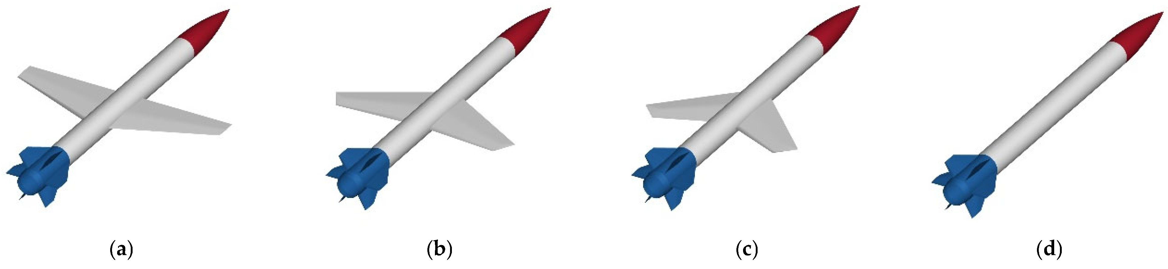
The morphing aircraft system consists of a fuselage and two wings, with the primary distinction being their structural rigidity. As the fuselage, equipped with six fins, is not prone to deformation, the fuselage is modeled as a rigid body capable of translational motion and rotational motion in space. In contrast, the wings, which account for almost 5% of the total aircraft mass, are regarded as straight beams [18] undergoing small elastic deformations and large overall motions following the fuselage, including variable-sweep rotations. Based on these characteristics, the morphing aircraft is modeled as a rigid–elastic coupling system integrating flight dynamics and structural dynamics.

(1)

Generalized Speeds

To describe aircraft motion, the American Coordinate System (ACS) for aircraft [19] is adopted, incorporating three coordinate frames in Figure 2: Earth-Fixed Coordinate System denoted by {I} (marked in red), Body-Fixed Coordinate System denoted by {B} (marked in cyan), and Velocity Coordinate System denoted by {V} (marked in green).

To describe translational motion, the position vector from the origin of {I} to O_F is denoted by ${\overrightarrow{\mathbf{R}}}_{{\mathrm{O}}_{\mathrm{F}}}$, while the velocity vector of the aircraft in {B} is ${\overrightarrow{\mathbf{V}}}_{{\mathrm{O}}_{\mathrm{F}}}$. Aircraft rotations are described using Euler angles ${\overrightarrow{\mathbf{\theta }}}_{\mathrm{F}}$ between {I} and {B}, with the angular rate vector ${\overrightarrow{\mathsf{\Omega }}}_{\mathrm{F}}$ in {B}. Their mathematical expressions are given as

$${}^I\overrightarrow{\mathit{R}}_{\mathit{OF}}={\left[x y z\right]}^{\mathrm{T}}, {}^B\overrightarrow{\mathit{V}}_{\mathit{OF}}={\left[u v w\right]}^{\mathrm{T}}$$

(2)

$${\overrightarrow{\mathit{\theta }}}_F={\left[\mathit{\varphi } \mathit{\theta } \mathit{\psi }\right]}^{\mathrm{T}}, {}^B\overrightarrow{\mathit{\Omega }}_F={\left[p q r\right]}^{\mathrm{T}}$$

(3)

where $\mathsf{\varphi }$, $\mathsf{\theta }$, and $\mathsf{\psi }$ denote the roll, pitch, and yaw angles, respectively.

To describe variable-sweep rotations of the left and right wings, the sweep angles of the two wings are denoted as ${\mathsf{\delta }}_{\mathrm{L}}$ and ${\mathsf{\delta }}_{\mathrm{R}}$, with the morphing rates denoted as ${\Lambda }_L$ and ${\Lambda }_{\mathrm{R}}$.

Elastic deformations are described using ${\eta }_{\mathrm{L}}$ and ${\eta }_{\mathrm{R}}$ as mode coordinates for neutral deformations of left and right beams and ${\mathsf{\zeta }}_{\mathrm{L}}$ and ${\mathsf{\zeta }}_{\mathrm{R}}$ as mode coordinates for lateral deformations of left and right beams. Then, their corresponding deformation rates are ${\dot{\eta }}_{\mathrm{L}},{\dot{\eta }}_{\mathrm{R}},{ \dot{\mathsf{\zeta }}}_{\mathrm{L}}$, and ${\dot{\mathsf{\zeta }}}_{\mathrm{R}}$.

To fully describe the system dynamics, $\mathrm{x},\mathrm{y},\mathrm{z},\mathsf{\varphi },\mathsf{\theta },\mathsf{\psi },{\mathsf{\delta }}_{\mathrm{L}},{\mathsf{\delta }}_{\mathrm{R}},{\mathsf{\eta }}_{\mathrm{L}},{\mathsf{\zeta }}_{\mathrm{L}},{\mathsf{\eta }}_{\mathrm{R}},{\mathrm{and} \mathsf{\zeta }}_{\mathrm{R}}$ are defined as twelve generalized coordinates, and $\mathrm{u},\mathrm{v},\mathrm{w},\mathrm{p},\mathrm{q},\mathrm{r},{\mathsf{\Lambda }}_{\mathrm{L}},{\mathsf{\Lambda }}_{\mathrm{R}},{\dot{\mathsf{\eta }}}_{\mathrm{L}},{\dot{\mathsf{\zeta }}}_{\mathrm{L}},{\dot{\mathsf{\eta }}}_{\mathrm{R}}, \mathrm{and}{\dot{\mathsf{\zeta }}}_{\mathrm{R}}$ as twelve generalized speeds.

(2)

Aircraft Kinematical Equations

Aircraft kinematics [20] and variable-sweep rotations can be described as follows:

$$\left\{\begin{array}{l}\dot{x}=u{C}_{\theta }{C}_{\psi }+v\left(S_{\theta }{C}_{\psi }{S}_{\varphi }-S_{\psi }{C}_{\varphi }\right)+w\left(S_{\theta }{C}_{\psi }{C}_{\varphi }+S_{\psi }{S}_{\varphi }\right)\\ \dot{y}=u{C}_{\theta }{S}_{\psi }+v\left(S_{\theta }{S}_{\psi }{S}_{\varphi }+C_{\psi }{C}_{\varphi }\right)+w\left(S_{\theta }{S}_{\psi }{C}_{\varphi }-C_{\psi }{S}_{\varphi }\right)\\ \dot{z}=-u{S}_{\theta }+v{C}_{\theta }{S}_{\varphi }+w{C}_{\theta }{C}_{\varphi }\\ \dot{\varphi }=p+\left(r{C}_{\varphi }+q{S}_{\varphi }\right)T_{\theta }\\ \dot{\theta }=q{C}_{\varphi }-r{S}_{\varphi }\\ \dot{\psi }=\left(r{C}_{\varphi }+q{S}_{\varphi }\right)/C_{\theta }\\ {\dot{\delta }}_L={\mathsf{\Lambda }}_L\\ {\dot{\delta }}_R={\mathsf{\Lambda }}_R\end{array}\right.$$

(4)

where ${\mathrm{S}}_{\mathsf{\theta }}=\sin \mathsf{\theta }$, ${\mathrm{C}}_{\mathsf{\theta }}=\cos \mathsf{\theta }$, and ${\mathrm{T}}_{\mathsf{\theta }}=\tan \mathsf{\theta }$.

(3)

Partial Angular Velocities

According to $\overrightarrow{{}^{\mathrm{B}}\mathbf{\Omega }_{\mathrm{F}}}$ in (3), twelve partial angular velocities of B_F are given by

$$\begin{array}{l}{{\overrightarrow{\omega }}_i}^F={\left[0 0 0\right]}^{\mathrm{T}} \mathrm{if} i<4,{{\overrightarrow{\omega }}_4}^F={\left[1 0 0\right]}^{\mathrm{T}},{{\overrightarrow{\omega }}_5}^F={\left[0 1 0\right]}^{\mathrm{T}}\\ {{\overrightarrow{\omega }}_6}^F={\left[0 0 1\right]}^{\mathrm{T}},{{\overrightarrow{\omega }}_i}^F={\left[0 0 0\right]}^{\mathrm{T}} \mathrm{if} i>6\end{array}$$

(5)

According to $\overrightarrow{{}^{\mathrm{B}}\mathbf{\Omega }_{\mathrm{R}}}={\left[p q r+{\mathsf{\Lambda }}_{\mathrm{R}}\right]}^{\mathrm{T}}$, twelve partial angular velocities of B_R are obtained.

$$\begin{array}{l}{{\overrightarrow{\omega }}_i}^R={\left[0 0 0\right]}^{\mathrm{T}} \mathrm{if} i<4,{{\overrightarrow{\omega }}_4}^R={\left[1 0 0\right]}^{\mathrm{T}},{{\overrightarrow{\omega }}_5}^R={\left[0 1 0\right]}^{\mathrm{T}},{{\overrightarrow{\omega }}_6}^R={\left[0 0 1\right]}^{\mathrm{T}}\\ {{\overrightarrow{\omega }}_7}^R={\left[0 0 0\right]}^{\mathrm{T}},{{\overrightarrow{\omega }}_8}^R={\left[0 0 1\right]}^{\mathrm{T}},{{\overrightarrow{\omega }}_i}^R={\left[0 0 0\right]}^{\mathrm{T}} \mathrm{if} i>8\end{array}$$

(6)

According to $\overrightarrow{{}^{\mathrm{B}}\mathbf{\Omega }_{\mathrm{L}}}={\left[p q r-{\mathsf{\Lambda }}_{\mathrm{L}}\right]}^{\mathrm{T}}$, twelve partial angular velocities of B_L are obtained.

$$\begin{array}{l}{{\overrightarrow{\omega }}_i}^L={\left[0 0 0\right]}^{\mathrm{T}} \mathrm{if} i<4,{{\overrightarrow{\omega }}_4}^L={\left[1 0 0\right]}^{\mathrm{T}},{{\overrightarrow{\omega }}_5}^L={\left[0 1 0\right]}^{\mathrm{T}}\\ {{\overrightarrow{\omega }}_6}^L={\left[0 0 1\right]}^{\mathrm{T}},{{\overrightarrow{\omega }}_7}^L={\left[0 0-1\right]}^{\mathrm{T}},{{\overrightarrow{\omega }}_i}^L={\left[0 0 0\right]}^{\mathrm{T}} \mathrm{if} i>7\end{array}$$

(7)

(4)

Partial Velocities

According to $\overrightarrow{{}^{\mathrm{B}}\mathrm{V}_{{\mathrm{O}}_{\mathrm{F}}}}$ in (2), twelve partial velocities of B_F are given by

$${{\overrightarrow{v}}_1}^F={\left[1 0 0\right]}^{\mathrm{T}}, {{\overrightarrow{v}}_2}^F={\left[0 1 0\right]}^{\mathrm{T}}, {{\overrightarrow{v}}_3}^F={\left[0 0 1\right]}^{\mathrm{T}},{{\overrightarrow{v}}_i}^F={\left[0 0 0\right]}^{\mathrm{T}}, i>3$$

(8)

To obtain partial velocities of B_R, we define ${\overrightarrow{\mathrm{V}}}_{{\mathrm{O}}_{\mathrm{R}}}$ as the absolute velocity vector below and then perform the discrete processing of elastic deformations.

$${\overrightarrow{V}}_{O_R}={\overrightarrow{V}}_{O_F}+{\overrightarrow{\Omega }}_F\times {\overrightarrow{\rho }}_{O_2}+{\overrightarrow{\Omega }}_R\times {\overrightarrow{\rho }}_R+{\dot{\overrightarrow{u}}}_R$$

(9)

where the COM of B_R is located at ${\mathrm{O}}_{\mathrm{R}}^{’}$ after elastic deformations. ${\overrightarrow{\mathbf{u}}}_{\mathrm{R}}$ denotes the elastic deformation vector from O_R to ${\mathrm{O}}_{\mathrm{R}}^{’}$, and it is expressed as ${\overrightarrow{\mathbf{u}}}_{\mathrm{R}}={\left[{\mathrm{u}}_1{\mathrm{u}}_2{\mathrm{u}}_3\right]}^{\mathrm{T}}$. u₁ denotes the axial deformation displacement of B_R. u₂ and u₃ are the lateral deformation displacements of B_R. ${\overrightarrow{\mathbf{\rho }}}_{{\mathrm{O}}_2}$ denotes the position vector from O_F to O₂. ${\overrightarrow{\mathit{\rho }}}_{O_2{O}_R}$ denotes the position vector from O₂ to O_R. ${\overrightarrow{\mathbf{\rho }}}_{\mathrm{R}}$ is the position vector and it is expressed as ${\overrightarrow{\mathbf{\rho }}}_{\mathrm{R}}={\overrightarrow{\mathbf{\rho }}}_{{\mathrm{O}}_2{\mathrm{O}}_{\mathrm{R}}}+{\overrightarrow{\mathbf{u}}}_{\mathrm{R}}$.

Next, the assumed mode method in [18] is employed to perform the discrete processing of elastic deformations. The results are given by

$$u_1={\varphi }_{11}{\eta }_R-\frac{1}{2}{K}_{n11}^3{{\zeta }_R}^2,u_2=0,u_3={\varphi }_{31}{\zeta }_R$$

(10)

where ${\mathsf{\varphi }}_{11}$ and ${\mathsf{\varphi }}_{31}$ are the vibration mode functions of B_R. ${\mathrm{K}}_{\mathrm{n}11}^3$ denotes the modal integration expressed as ${\mathrm{K}}_{\mathrm{n}11}^3={\int }_0^{{\mathrm{L}}_{\mathrm{W}}/2}{{\dot{\mathsf{\varphi }}}_{31}}^2\mathrm{dx}$.

According to (9) and (10), twelve partial velocities of B_R are given by

$$\begin{array}{l}{{\overrightarrow{v}}_4}^R=\left[\begin{array}{c}0\\ 0\\ {\mathrm{R}}_{\mathrm{B}}+C_{{\delta }_R}{\mathrm{L}}_{\mathrm{W}}/2\end{array}\right],{{\overrightarrow{v}}_5}^R=\left[\begin{array}{c}0\\ 0\\ -{\mathrm{X}}_{\mathrm{W}}+S_{{\delta }_R}{\mathrm{L}}_{\mathrm{W}}/2\end{array}\right],{{\overrightarrow{v}}_6}^R=\left[\begin{array}{c}-{\mathrm{R}}_{\mathrm{B}}-C_{{\delta }_R}{\mathrm{L}}_{\mathrm{W}}/2\\ {\mathrm{X}}_{\mathrm{W}}-S_{{\delta }_R}{\mathrm{L}}_{\mathrm{W}}/2\\ 0\end{array}\right],{{\overrightarrow{v}}_7}^R={\left[0 0 0\right]}^{\mathrm{T}}\\ {{\overrightarrow{v}}_8}^R=\left[\begin{array}{c}-C_{{\delta }_R}{\mathrm{L}}_{\mathrm{W}}/2\\ -S_{{\delta }_R}{\mathrm{L}}_{\mathrm{W}}/2\\ 0\end{array}\right],{{\overrightarrow{v}}_9}^R={{\overrightarrow{v}}_{10}}^R={\left[0 0 0\right]}^{\mathrm{T}},{\overrightarrow{v}}_{11}^R=\left[\begin{array}{c}{\varphi }_{11}\\ 0\\ 0\end{array}\right],{\overrightarrow{v}}_{12}^R=\left[\begin{array}{c}-K_{n11}^3{\zeta }_R\\ 0\\ {\varphi }_{31}\end{array}\right]\end{array}$$

(11)

where ${\mathrm{S}}_{{\mathsf{\delta }}_{\mathrm{R}}}=\sin {\mathsf{\delta }}_{\mathrm{R}}$ and ${\mathrm{C}}_{{\mathsf{\delta }}_{\mathrm{R}}}=\cos {\mathsf{\delta }}_{\mathrm{R}}$.

Similarly, ${\overrightarrow{\mathrm{V}}}_{{\mathrm{O}}_{\mathrm{L}}}$ is defined as the absolute velocity vector of B_L. Then, the assumed mode method in [18] is employed for the discrete processing of elastic deformations. The results are given by

$$u_{L1}={\varphi }_{11\_sys}{\eta }_L-\frac{1}{2}{K}_{Ln11}^3{{\zeta }_L}^2,u_{L2}=0,u_{L3}={\varphi }_{31\_sys}{\zeta }_L$$

(12)

where ${\varphi }_{11\_sys}$ and ${\varphi }_{31\_sys}$ are the vibration mode functions of B_L. ${\mathrm{K}}_{\mathrm{n}11}^3$ denotes the modal integration expressed as ${\mathrm{K}}_{\mathrm{Ln}11}^3={\int }_{-{\mathrm{L}}_{\mathrm{W}}/2}^0{{\dot{\mathsf{\varphi }}}_{31\_\mathrm{sys}}}^2\mathrm{dx}$.

According to ${\overrightarrow{\mathrm{V}}}_{{\mathrm{O}}_{\mathrm{L}}}$ and (12), twelve partial velocities of B_L are given by

$$\begin{array}{l}{{\overrightarrow{v}}_1}^L={\left[1 0 0\right]}^{\mathrm{T}},{{\overrightarrow{v}}_2}^L={\left[0 1 0\right]}^{\mathrm{T}},{{\overrightarrow{v}}_3}^L={\left[0 0 1\right]}^{\mathrm{T}},{{\overrightarrow{v}}_4}^L=\left[\begin{array}{c}0\\ 0\\ -{\mathrm{R}}_{\mathrm{B}}-C_{{\delta }_L}{\mathrm{L}}_{\mathrm{W}}/2\end{array}\right],{{\overrightarrow{v}}_5}^L=\left[\begin{array}{c}0\\ 0\\ -{\mathrm{X}}_{\mathrm{W}}+S_{{\delta }_L}{\mathrm{L}}_{\mathrm{W}}/2\end{array}\right],{{\overrightarrow{v}}_6}^L=\left[\begin{array}{c}{\mathrm{R}}_{\mathrm{B}}+C_{{\delta }_L}{\mathrm{L}}_{\mathrm{W}}/2\\ {\mathrm{X}}_{\mathrm{W}}-S_{{\delta }_L}{\mathrm{L}}_{\mathrm{W}}/2\\ 0\end{array}\right]\\ {{\overrightarrow{v}}_7}^L=\left[\begin{array}{c}-C_{{\delta }_L}{\mathrm{L}}_{\mathrm{W}}/2\\ S_{{\delta }_L}{\mathrm{L}}_{\mathrm{W}}/2\\ 0\end{array}\right],{{\overrightarrow{v}}_8}^L={\left[0 0 0\right]}^{\mathrm{T}},{{\overrightarrow{v}}_9}^L=\left[\begin{array}{c}{\varphi }_{11\_sys}\\ 0\\ 0\end{array}\right],{{\overrightarrow{v}}_{10}}^L=\left[\begin{array}{c}-K_{Ln11}^3{\zeta }_L\\ 0\\ {\varphi }_{31\_sys}\end{array}\right],{{\overrightarrow{v}}_{11}}^L={{\overrightarrow{v}}_{12}}^L={\left[0 0 0\right]}^{\mathrm{T}}\end{array}$$

(13)

where $S_{{\delta }_L}=\mathit{sin}{\delta }_L$ and ${\mathrm{C}}_{{\mathsf{\delta }}_{\mathrm{L}}}=\cos {\mathsf{\delta }}_{\mathrm{L}}$.

To enhance readability when applying Kane’s method,

Table 7. Generalized forces of a rigid–elastic coupling system.

Generalized Forces	Part	Forces	Moments	Motion
Inertia force	BF	Inertia force, ${\overrightarrow{R}}_F^{\ast }$	Inertia torque, ${\overrightarrow{T}}_F^{\ast }$	Translation, rotation
	BR	Inertia force, ${\overrightarrow{R}}_R^{\ast }$	Inertia torque, ${\overrightarrow{T}}_R^{\ast }$	Uncertainty
	BL	Inertia force, ${\overrightarrow{R}}_L^{\ast }$	Inertia torque, ${\overrightarrow{T}}_L^{\ast }$	Uncertainty
Active force	BF	Aerodynamic force, ${\overrightarrow{F}}_A$	Aerodynamic moments, ${\overrightarrow{M}}_A$	Translation, rotation
		Engine thrust, ${\overrightarrow{P}}_F$	Motor torque, ${\overrightarrow{M}}_{FW}$	Translation
		Gravity, ${\overrightarrow{G}}_F$		Translation
	BR	Gravity, ${\overrightarrow{G}}_w$	Motor torque, ${\overrightarrow{M}}_{RF}$	Variable-sweep rotation
	BL	Gravity, ${\overrightarrow{G}}_w$	Motor torque, ${\overrightarrow{M}}_{LF}$	Variable-sweep rotation
Internal force	BF	Generalized internal forces, $F_{Fr}^{in}=0\begin{array}{}\end{array}(r=1,...,12)$		No vibration
	BR	Generalized internal forces, $F_{Rr}^{in}\begin{array}{}\end{array}(r=1,...,12)$		Elastic vibration, uncertainty
	BL	Generalized internal forces, $F_{Lr}^{in}\begin{array}{}\end{array}(r=1,...,12)$		Elastic vibration, uncertainty

defines the forces and moments contributing to the generalized forces of the coupled system. The generalized forces acting on the fuselage drive translational and rotational motions without introducing uncertainties, whereas those acting on the wings induce variable-sweep rotations, elastic vibrations, and associated uncertainties.

3.2. Generalized Inertia Forces

The inertia force and inertia torque of B_F can be described as

$${\overrightarrow{R}}_F^{\ast }=-m_F\cdot {\overrightarrow{a}}_{O_F}$$

(14)

$${\overrightarrow{T}}_F^{\ast }=-J_F\cdot {\dot{\overrightarrow{\Omega }}}_F-{\overrightarrow{\Omega }}_F\times \left(J_F\cdot {\overrightarrow{\Omega }}_F\right)$$

(15)

where ${\overrightarrow{\mathrm{a}}}_{{\mathrm{O}}_{\mathrm{F}}}$ is the COM acceleration of B_F, and it is expressed as ${\overrightarrow{\mathrm{a}}}_{{\mathrm{O}}_{\mathrm{F}}}\triangleq {\dot{\overrightarrow{\mathrm{V}}}}_{{\mathrm{O}}_{\mathrm{F}}}$.

Considering (5), (8), (14) and (15), the contribution of B_F to the aircraft’s generalized inertial force is given by

$$F_{Fr}^{\ast }={{\overrightarrow{\omega }}_r}^F\cdot {\overrightarrow{T}}_F^{\ast }+{{\overrightarrow{v}}_r}^F\cdot {\overrightarrow{R}}_F^{\ast } (r=1,...,12)$$

(16)

The inertia force and inertia torque of B_R can be described as

$${\overrightarrow{R}}_R^{\ast }=-m_W\cdot {\overrightarrow{a}}_{O_R}$$

(17)

$${\overrightarrow{T}}_R^{\ast }=-J_W\cdot {\dot{\overrightarrow{\Omega }}}_R-{\overrightarrow{\Omega }}_R\times \left(J_W\cdot {\overrightarrow{\Omega }}_R\right)$$

(18)

where ${\overrightarrow{\mathrm{a}}}_{{\mathrm{O}}_{\mathrm{R}}}$ denotes the COM acceleration of B_R, and it is expressed as ${\overrightarrow{\mathrm{a}}}_{{\mathrm{O}}_{\mathrm{R}}}\triangleq {\dot{\overrightarrow{\mathrm{V}}}}_{{\mathrm{O}}_{\mathrm{R}}}$.

Considering (6), (11), (17) and (18), the contribution of B_R to the aircraft’s generalized inertial force is given by

$$F_{Rr}^{\ast }={{\overrightarrow{\omega }}_r}^R\cdot {\overrightarrow{T}}_R^{\ast }+{{\overrightarrow{v}}_r}^R\cdot {\overrightarrow{R}}_R^{\ast } (r=1,...,12)$$

(19)

Similarly, ${\overrightarrow{\mathrm{a}}}_{{\mathrm{O}}_{\mathrm{L}}}$ is defined as the COM acceleration of B_L, and it is expressed as ${\overrightarrow{\mathrm{a}}}_{{\mathrm{O}}_{\mathrm{L}}}\triangleq {\dot{\overrightarrow{\mathrm{V}}}}_{{\mathrm{O}}_{\mathrm{L}}}$. Then, the inertia force and inertia torque of B_L can be obtained.

$${\overrightarrow{R}}_L^{\ast }=-m_W\cdot {\overrightarrow{a}}_{O_L}$$

(20)

$${\overrightarrow{T}}_L^{\ast }=-J_W\cdot {\dot{\overrightarrow{\Omega }}}_L-{\overrightarrow{\Omega }}_L\times \left(J_W\cdot {\overrightarrow{\Omega }}_L\right)$$

(21)

Considering (7), (13), (20) and (21), the contribution of B_L to the aircraft’s generalized inertial force is given by

$$F_{Lr}^{\ast }={{\overrightarrow{\omega }}_r}^L\cdot {\overrightarrow{T}}_L^{\ast }+{{\overrightarrow{v}}_r}^L\cdot {\overrightarrow{R}}_L^{\ast } (r=1,...,12)$$

(22)

Considering (16), (19) and (22), the aircraft’s generalized inertial force is given by

$$F_r^{\ast }=F_{Fr}^{\ast }+F_{Rr}^{\ast }+F_{Lr}^{\ast } (r=1,...,12)$$

(23)

3.3. Generalized Active Forces

The aerodynamic force on each part is expressed in {V}, while the engine thrust and gravity are expressed in {B} and {I}, below. Then, we obtain

$${}^V\overrightarrow{F}_A=\left[\begin{array}{c}-D\\ Y\\ -L\end{array}\right],{}^B\overrightarrow{P}_F=\left[\begin{array}{c}P\\ 0\\ 0\end{array}\right],{}^I\overrightarrow{G}_F=\left[\begin{array}{c}0\\ 0\\ m_{F}g\end{array}\right],{}^I\overrightarrow{G}_w=\left[\begin{array}{c}0\\ 0\\ m_{W}g\end{array}\right]$$

(24)

Aerodynamic moments and motor torque are all expressed in {B}. Then, we obtain

$${}^B\overrightarrow{M}_A=\left[\begin{array}{c}{M}_x\\ M_y\\ M_z\end{array}\right],{}^B\overrightarrow{M}_{RF}=\left[\begin{array}{c}0\\ 0\\ -T_R\end{array}\right],{}^B\overrightarrow{M}_{LF}=\left[\begin{array}{c}0\\ 0\\ -T_L\end{array}\right],{}^B\overrightarrow{M}_{FW}=\left[\begin{array}{c}0\\ 0\\ T_L+T_R\end{array}\right]$$

(25)

Considering (24) and (25), the active force and the active moment on B_F are given by

$${\overrightarrow{R}}_F={\overrightarrow{F}}_A+{\overrightarrow{G}}_F+{\overrightarrow{P}}_F, {\overrightarrow{T}}_F={\overrightarrow{M}}_A+{\overrightarrow{M}}_{FW}$$

(26)

Based on (5), (8) and (26), the contribution of B_F to the aircraft’s generalized active force is given by

$$F_{Fr}^{ac}={{\overrightarrow{\omega }}_r}^F\cdot {\overrightarrow{T}}_F+{{\overrightarrow{v}}_r}^F\cdot {\overrightarrow{R}}_F (r=1,...,12)$$

(27)

Considering (24) and (25), the active force and the active moment on B_R are given by

$${\overrightarrow{R}}_R={}^I\overrightarrow{G}_w,{\overrightarrow{T}}_R={}^B\overrightarrow{M}_{\mathit{RF}}$$

(28)

Based on (6), (11) and (28), the contribution of B_R to the aircraft’s generalized active force is given by

$$F_{Rr}^{ac}={{\overrightarrow{\omega }}_r}^R\cdot {\overrightarrow{T}}_R+{{\overrightarrow{v}}_r}^R\cdot {\overrightarrow{R}}_R (r=1,...,12)$$

(29)

Similarly, considering (24) and (25), the active force and the active moment on B_L are given by

$${\overrightarrow{R}}_L={}^I\overrightarrow{G}_w,{\overrightarrow{T}}_L={\overrightarrow{M}}_{LF}$$

(30)

Based on (7), (13) and (30), the contribution of B_L to the aircraft’s generalized active force is given by

$$F_{Lr}^{ac}={{\overrightarrow{\omega }}_r}^L\cdot {\overrightarrow{T}}_L+{{\overrightarrow{v}}_r}^L\cdot {\overrightarrow{R}}_L (r=1,...,12)$$

(31)

Considering (27), (29) and (31), the aircraft’s generalized active force is given by

$$F_r^{ac}=F_{Fr}^{ac}+F_{Rr}^{ac}+F_{Lr}^{ac} (r=1,...,12)$$

(32)

3.4. Generalized Internal Forces

As B_F is rigid, there is no elastic force on it, and the contribution of B_F to the aircraft’s generalized internal force is given by

$$F_{Fr}^{in}=0 (r=1,...,12)$$

(33)

However, B_R and B_L are modeled as elastic beams. According to the strain energy 18 of the straight beams, the contribution of B_R to the aircraft’s generalized internal force is given by

$$F_{Rr}^{in}=F_{Lr}^{in}=0 (r=1,...,10),F_{R11}^{in}=-K_{11}^1{\eta }_R,F_{R12}^{in}=-K_{11}^3{\zeta }_R$$

(34)

where ${\mathrm{K}}_{11}^1 \mathrm{and}{ \mathrm{K}}_{11}^3$ denote modal integrations, and they are expressed as

$$K_{11}^1={\displaystyle {\int }_0^{{\mathrm{L}}_{\mathrm{W}}/2}EA{{\dot{\varphi }}_{11}}^{2}dx},K_{11}^3={\displaystyle {\int }_0^{{\mathrm{L}}_{\mathrm{W}}/2}E{I}_3{{\ddot{\varphi }}_{31}}^{2}dx}$$

(35)

Similarly, the contribution of B_L to the aircraft’s generalized internal force is given by

$$F_{Lr}^{in}=0 (r=1,...,8,11,12),F_{L9}^{in}=-K_{L11}^1{\eta }_L,F_{L10}^{in}=-K_{L11}^3{\zeta }_L$$

(36)

where ${\mathrm{K}}_{\mathrm{L}11}^1 \mathrm{and}{\mathrm{K}}_{\mathrm{L}11}^3$ denote modal integrations, and they are expressed as

$$K_{L11}^1={\displaystyle {\int }_{-{\mathrm{L}}_{\mathrm{W}}/2}^{0}EA{{\dot{\varphi }}_{11\_sys}}^{2}dx},K_{L11}^3={\displaystyle {\int }_{-{\mathrm{L}}_{\mathrm{W}}/2}^{0}E{I}_3{{\ddot{\varphi }}_{31\_sys}}^{2}dx}$$

(37)

where $E, A,\mathrm{a}\mathrm{n}\mathrm{d} I_3$ denote Young’s modulus, the cross-sectional area, and the area moment of inertia of B_R and B_L.

Considering (33), (34) and (36), the aircraft’s generalized internal force is given by

$$F_r^{in}=F_{Fr}^{in}+F_{Rr}^{in}+F_{Lr}^{in} (r=1,...,12)$$

(38)

3.5. Rigid–Elastic Coupling Dynamics

Using the twelve generalized coordinates and speeds in Section 3.1, the twelve partial angular velocities and twelve partial velocities for each component of the variable-sweep aircraft are derived. By incorporating generalized inertial forces in Section 3.2, generalized active forces in Section 3.3, and generalized internal forces in Section 3.4, the twelve Kane dynamic equations, describing flight dynamics and structural dynamics, are obtained as

$$F_r^{\ast }+F_r^{ac}+F_r^{in}=0 (r=1,...,12)$$

(39)

Assuming symmetric and uniform wings (${\mathsf{\delta }}_{\mathrm{L}}={\mathsf{\delta }}_{\mathrm{R}}={\mathsf{\delta }}_{\mathrm{w}}$, ${\dot{\mathsf{\Lambda }}}_{\mathrm{L}}={\dot{\mathsf{\Lambda }}}_{\mathrm{R}}=\dot{\mathsf{\Lambda }}=0$), the rigid–elastic coupling dynamic model of the variable-sweep aircraft is established from (40)–(46), where $S_{\alpha }=\mathit{sin}\alpha$, $C_{\alpha }=\mathit{cos}\alpha$, $S_{\beta }=\mathit{sin}\beta$, and $C_{\beta }=\mathit{cos}\beta$ are defined to facilitate the equation’s expression. The state variables of the Kane dynamic equations consist of the twelve generalized speeds. However, the state variables of the kinematic equations consist of the twelve generalized coordinates.

The eight flight dynamics in Equation (40) consist of translation, rotation, and variable-sweep rotation dynamics. The eight flight kinematics in Equation (41) describe translation, rotation, and variable-sweep kinematics.

Furthermore, the four structural dynamics in Equations (42)–(45) govern the elastic deformations of the two beams, and the four kinematics equations of elastic vibrations (46) describe the deformation rates.

In addition, the coupling terms (40) represent model uncertainties arising from two primary sources:

(1)

Variable-sweep rotations (marked with _) are expressed in (47) and (49), distinguishing these uncertainties from traditional rigid-body dynamics.

(2)

Elastic deformations (marked with _) are expressed in (48) and (50), differentiating their uncertainties from conventional multibody dynamics.

$$\left\{\begin{array}{l}m\left(\dot{u}+wq-vr\right)=-mg{S}_{\theta }-D{C}_{\alpha }{C}_{\beta }-Y{C}_{\alpha }{S}_{\beta }+L{S}_{\alpha }+P+\underset{¯}{F_{mor\_x}}+\underset{¯}{\underset{¯}{F_{ela\_x}}}\\ m\left(\dot{v}+ur-wp\right)=mg{C}_{\theta }{S}_{\varphi }-D{S}_{\beta }+Y{C}_{\beta }+\underset{¯}{F_{mor\_y}}+\underset{¯}{\underset{¯}{F_{ela\_y}}}\\ m\left(\dot{w}+vp-uq\right)=mg{C}_{\theta }{C}_{\varphi }-D{S}_{\alpha }{C}_{\beta }-Y{S}_{\alpha }{S}_{\beta }-L{C}_{\alpha }+\underset{¯}{F_{mor\_z}}+\underset{¯}{\underset{¯}{F_{ela\_z}}}\\ \dot{p}{J}_{Fx}-qr\left(J_{Fy}-J_{Fz}\right)=M_x+\underset{¯}{M_{mor\_x}}+\underset{¯}{\underset{¯}{M_{ela\_x}}}\\ \dot{q}{J}_{Fy}-rp\left(J_{Fz}-J_{Fx}\right)=M_y+\underset{¯}{M_{mor\_y}}+\underset{¯}{\underset{¯}{M_{ela\_y}}}\\ \dot{r}{J}_{Fz}-pq\left(J_{Fx}-J_{Fy}\right)=M_z+\underset{¯}{M_{mor\_z}}+\underset{¯}{\underset{¯}{M_{ela\_z}}}\\ {\dot{\mathsf{\Lambda }}}_L=\dot{\mathsf{\Lambda }}=0\\ {\dot{\mathsf{\Lambda }}}_R=\dot{\mathsf{\Lambda }}=0\end{array}\right.$$

(40)

where $F_{\mathit{mor}\_\mathit{x}},F_{\mathit{mor}\_\mathit{y}},\mathrm{and}{F}_{\mathit{mor}\_\mathit{z}}$ denote additional morphing forces. $F_{\mathit{ela}\_\mathit{x}},F_{\mathit{ela}\_\mathit{y}},{\mathrm{and}F}_{\mathit{ela}\_\mathit{z}}$ denote additional elastic forces. $M_{\mathit{mor}\_\mathit{x}},M_{\mathit{mor}\_\mathit{y}},{\mathrm{and}M}_{\mathit{mor}\_\mathit{z}}$ denote additional morphing moments. $M_{\mathit{ela}\_\mathit{x}},M_{\mathit{ela}\_\mathit{y}},{\mathrm{and}M}_{\mathit{ela}\_\mathit{z}}$ denote additional elastic moments.

$$\left\{\begin{array}{l}\dot{x}=u{C}_{\theta }{C}_{\psi }+v\left(S_{\theta }{C}_{\psi }{S}_{\varphi }-S_{\psi }{C}_{\varphi }\right)+w\left(S_{\theta }{C}_{\psi }{C}_{\varphi }+S_{\psi }{S}_{\varphi }\right)\\ \dot{y}=u{C}_{\theta }{S}_{\psi }+v\left(S_{\theta }{S}_{\psi }{S}_{\varphi }+C_{\psi }{C}_{\varphi }\right)+w\left(S_{\theta }{S}_{\psi }{C}_{\varphi }-C_{\psi }{S}_{\varphi }\right)\\ \dot{z}=-u{S}_{\theta }+v{C}_{\theta }{S}_{\varphi }+w{C}_{\theta }{C}_{\varphi }\\ \dot{\varphi }=p+\left(r{C}_{\varphi }+q{S}_{\varphi }\right)T_{\theta }\\ \dot{\theta }=q{C}_{\varphi }-r{S}_{\varphi }\\ \dot{\psi }=\left(r{C}_{\varphi }+q{S}_{\varphi }\right)/C_{\theta }\\ {\dot{\delta }}_L={\dot{\delta }}_w=\mathsf{\Lambda }\\ {\dot{\delta }}_R={\dot{\delta }}_w=\mathsf{\Lambda }\end{array}\right.$$

(41)

$$m_W{{\varphi }_{11\_sys}}^2{\ddot{\eta }}_L=-m_{W}g{S}_{\theta }{\varphi }_{11\_sys}-K_{L11}^1{\eta }_L-m_W{\varphi }_{11\_sys}\left[\begin{array}{l}\dot{u}+wq-vr+\dot{r}\left({\mathrm{R}}_{\mathrm{B}}+C_{\delta }{\mathrm{L}}_{\mathrm{W}}/2\right)+pq\left({\mathrm{R}}_{\mathrm{B}}-C_{\delta }{\mathrm{L}}_{\mathrm{W}}/2\right)\\ {+\mathrm{X}}_{\mathrm{W}}\left(q^2-r^2\right)+S_{\delta }{\mathrm{L}}_{\mathrm{W}}\left(q^2+r^2+{\mathsf{\Lambda }}^2-2r\mathsf{\Lambda }\right)/2\\ +2q{\varphi }_{31\_sys}{\dot{\zeta }}_L-K_{Ln11}^3\left({\dot{\zeta }}_L{\ddot{\zeta }}_L+{{\dot{\zeta }}_L}^2+{\zeta }_L{\ddot{\zeta }}_L\right)\end{array}\right]$$

(42)

$$\begin{array}{cc}{m}_W{{\varphi }_{31\_sys}}^2{\ddot{\zeta }}_L& =m_{W}g{S}_{\theta }\left(K_{Ln11}^3{\zeta }_L+C_{\theta }{C}_{\varphi }{\varphi }_{31\_sys}\right)\\ & -K_{L11}^3{\zeta }_L+m_W{K}_{Ln11}^3{\zeta }_L\left[\begin{array}{l}\dot{u}+wq-vr+\dot{r}\left({\mathrm{R}}_{\mathrm{B}}+C_{\delta }{\mathrm{L}}_{\mathrm{W}}/2\right)+pq\left({\mathrm{R}}_{\mathrm{B}}-C_{\delta }{\mathrm{L}}_{\mathrm{W}}/2\right)\\ {+\mathrm{X}}_{\mathrm{W}}\left(q^2-r^2\right)+S_{\delta }{\mathrm{L}}_{\mathrm{W}}\left(q^2+r^2+{\mathsf{\Lambda }}^2-2r\mathsf{\Lambda }\right)/2\\ +2q{\varphi }_{31\_sys}{\dot{\zeta }}_L+{\varphi }_{11\_sys}{\ddot{\eta }}_L-K_{Ln11}^3\left({\dot{\zeta }}_L{\ddot{\zeta }}_L+{{\dot{\zeta }}_L}^2+{\zeta }_L{\ddot{\zeta }}_L\right)\end{array}\right]\\ & -m_W{\varphi }_{31\_sys}\left[\begin{array}{l}\dot{w}+vp-uq-\dot{q}\left({\mathrm{X}}_{\mathrm{W}}+S_{\delta }{\mathrm{L}}_{\mathrm{W}}/2\right)-\dot{p}\left({\mathrm{R}}_{\mathrm{B}}+C_{\delta }{\mathrm{L}}_{\mathrm{W}}/2\right)\\ +pr\left({\mathrm{X}}_{\mathrm{W}}-S_{\delta }{\mathrm{L}}_{\mathrm{W}}/2\right)-qr\left({\mathrm{R}}_{\mathrm{B}}+C_{\delta }{\mathrm{L}}_{\mathrm{W}}/2\right)+\mathsf{\Lambda }{\mathrm{L}}_{\mathrm{W}}\left(p{S}_{\delta }+q{C}_{\delta }\right)/2\\ -2q\left({\varphi }_{11\_sys}{\dot{\eta }}_L-K_{Ln11}^3{\zeta }_L{\dot{\zeta }}_L\right)\end{array}\right]\end{array}$$

(43)

$$m_W{{\varphi }_{11}}^2{\ddot{\eta }}_R=-m_{W}g{S}_{\theta }{\varphi }_{11}-K_{11}^1{\eta }_R-m_W{\varphi }_{11}\left[\begin{array}{l}\dot{u}+wq-vr+\left(pq-\dot{r}\right)\left({\mathrm{R}}_{\mathrm{B}}+C_{\delta }{\mathrm{L}}_{\mathrm{W}}/2\right)\\ -{\mathrm{X}}_{\mathrm{W}}\left(r^2+q^2\right)+S_{\delta }{\mathrm{L}}_{\mathrm{W}}\left(q^2+r^2+{\mathsf{\Lambda }}^2+2r\mathsf{\Lambda }\right)/2\\ +2q{\varphi }_{31}{\dot{\zeta }}_R-K_{n11}^3\left({\dot{\zeta }}_R{\ddot{\zeta }}_R+{{\dot{\zeta }}_R}^2+{\zeta }_R{\ddot{\zeta }}_R\right)\end{array}\right]$$

(44)

$$\begin{array}{cc}{m}_W{{\varphi }_{31}}^2{\ddot{\zeta }}_R& =m_{W}g\left(S_{\theta }{K}_{n11}^3{\zeta }_R+C_{\theta }{C}_{\varphi }{\varphi }_{31}\right)-K_{11}^3{\zeta }_R+m_W{K}_{n11}^3{\zeta }_R\left[\begin{array}{l}\dot{u}+wq-vr+\left(pq-\dot{r}\right)\left({\mathrm{R}}_{\mathrm{B}}+C_{\delta }{\mathrm{L}}_{\mathrm{W}}/2\right)\\ -{\mathrm{X}}_{\mathrm{W}}\left(r^2+q^2\right)+\left(q^2+r^2+{\mathsf{\Lambda }}^2+2r\mathsf{\Lambda }\right)S_{\delta }{\mathrm{L}}_{\mathrm{W}}/2\\ +2q{\varphi }_{31}{\dot{\zeta }}_R+{\varphi }_{11}{\ddot{\eta }}_R-K_{n11}^3\left({\dot{\zeta }}_R{\ddot{\zeta }}_R+{{\dot{\zeta }}_R}^2+{\zeta }_R{\ddot{\zeta }}_R\right)\end{array}\right]\\ & -m_W{\varphi }_{31}\left[\begin{array}{l}\dot{w}+vp-uq+\left(\dot{q}-pr\right)\left(S_{\delta }{\mathrm{L}}_{\mathrm{W}}/2-{\mathrm{X}}_{\mathrm{W}}\right)\\ +\left(\dot{p}+qr\right)\left({\mathrm{R}}_{\mathrm{B}}+C_{\delta }{\mathrm{L}}_{\mathrm{W}}/2\right)+\mathsf{\Lambda }{\mathrm{L}}_{\mathrm{W}}\left(q{C}_{\delta }-p{S}_{\delta }\right)/2\\ -2q\left({\varphi }_{11}{\dot{\eta }}_R-K_{n11}^3{\zeta }_R{\dot{\zeta }}_R\right)\end{array}\right]\end{array}$$

(45)

$${\dot{\eta }}_L={\dot{\eta }}_L,{\dot{\zeta }}_L={\dot{\zeta }}_L,{\dot{\eta }}_R={\dot{\eta }}_R,{\dot{\zeta }}_R={\dot{\zeta }}_R$$

(46)

The complexity of the proposed rigid–elastic coupling dynamic model arises from the intricate interaction between rigid-body dynamics, variable-sweep rotations, and elastic deformations, all of which introduce model uncertainties. The wings undergoing variable-sweep rotations generate additional morphing force and additional morphing moment in (40), while the wings undergoing elastic deformations generate additional elastic force and additional elastic moment in (40).

In (40), $F_{\mathit{mor}\_\mathit{x}},F_{\mathit{mor}\_\mathit{y}},{\mathrm{and} F}_{\mathit{mor}\_\mathit{z}}$ are model uncertainties due to variable-sweep rotations of the two wings. This morphing process alters their COM positions and inertia forces. There are derivative relationships between the position vector, velocity vector, and acceleration vector. According to (9), variations in the COM position lead to additional COM velocities and accelerations. As derived in (17), these extra COM accelerations further contribute to additional inertia forces. Consequently, the variations in the COM position of the two wings contribute to the aircraft’s generalized inertia forces, as shown in (19). In addition, the large-scale variations in aerodynamic forces caused by variable-sweep configurations change aircraft translations. $F_{\mathit{mor}\_\mathit{x}},F_{\mathit{mor}\_\mathit{y}},\mathrm{and}{F}_{\mathit{mor}\_\mathit{z}}$ are expressed as

$$\left\{\begin{array}{l}{F}_{mor\_x}=-m_W\left[2qp{\mathrm{R}}_{\mathrm{B}}-2r^2{\mathrm{X}}_{\mathrm{W}}+{\mathrm{L}}_{\mathrm{W}}{S}_{\delta }\left(q^2+r^2+{\mathsf{\Lambda }}^2\right)\right]\\ F_{mor\_y}=-m_W\left[\left(\dot{r}+pq\right)\left(2{\mathrm{X}}_{\mathrm{W}}-S_{\delta }{\mathrm{L}}_{\mathrm{W}}\right)-2r\mathsf{\Lambda }{C}_{\delta }{\mathrm{L}}_{\mathrm{W}}\right]\\ F_{mor\_z}=-m_W\left[\left(pr-\dot{q}\right)\left(2{\mathrm{X}}_{\mathrm{W}}-S_{\delta }{\mathrm{L}}_{\mathrm{W}}\right)+q\mathsf{\Lambda }{C}_{\delta }{\mathrm{L}}_{\mathrm{W}}\right]\end{array}\right.$$

(47)

In (40), $F_{\mathit{ela}\_\mathit{x}},F_{\mathit{ela}\_\mathit{y}},{\mathrm{and}F}_{\mathit{ela}\_\mathit{z}}$ are model uncertainties caused by the elastic deformations of the two wings. The elastic deformations alter their deformation displacements of COM, inertia forces, and internal forces. As shown in (9), both axial and lateral deformations induce extra deformation velocities and accelerations. According to (17), extra deformation accelerations develop extra inertia force. According to (19), the elastic deformations of the two wings contribute to the aircraft’s generalized inertia forces. In addition, the small elastic deformations contribute to the aircraft’s generalized internal forces according to (34). These factors will trigger elastic vibrations and alter the translational motions of the aircraft. $F_{\mathit{ela}\_\mathit{x}},F_{\mathit{ela}\_\mathit{y}},{\mathrm{and}F}_{\mathit{ela}\_\mathit{z}}$ are expressed as

$$\left\{\begin{array}{l}{F}_{ela\_x}=-m_W\left[2q\left({\varphi }_{31\_sys}{\dot{\zeta }}_L+{\varphi }_{31}{\dot{\zeta }}_R\right)+{\varphi }_{11\_sys}{\ddot{\eta }}_L+{\varphi }_{11}{\ddot{\eta }}_R-K_{Lu11}\left({\dot{\zeta }}_L{\ddot{\zeta }}_L+{{\dot{\zeta }}_L}^2+{\zeta }_L{\ddot{\zeta }}_L\right)-K_{u11}\left({\dot{\zeta }}_R{\ddot{\zeta }}_R+{{\dot{\zeta }}_R}^2+{\zeta }_R{\ddot{\zeta }}_R\right)\right]\\ F_{ela\_y}=-m_W\left[2\left(r-\mathsf{\Lambda }\right)\left({\varphi }_{11\_sys}{\dot{\eta }}_L-K_{Lu11}{\zeta }_L{\dot{\zeta }}_L\right)+2\left(r+\mathsf{\Lambda }\right)\left({\varphi }_{11}{\dot{\eta }}_R-K_{u11}{\zeta }_R{\dot{\zeta }}_R\right)-2p\left({\varphi }_{31\_sys}{\dot{\zeta }}_L+{\varphi }_{31}{\dot{\zeta }}_R\right)\right]\\ F_{ela\_z}=-m_W\left[-2q\left({\varphi }_{11\_sys}{\dot{\eta }}_L-K_{Lu11}{\zeta }_L{\dot{\zeta }}_L+{\varphi }_{11}{\dot{\eta }}_R-K_{u11}{\zeta }_R{\dot{\zeta }}_R\right)+{\varphi }_{31\_sys}{\ddot{\zeta }}_L+{\varphi }_{31}{\ddot{\zeta }}_R\right]\end{array}\right.$$

(48)

In (40), $M_{\mathit{mor}\_\mathit{x}},M_{\mathit{mor}\_\mathit{y}},{\mathrm{and} M}_{\mathit{mor}\_\mathit{z}}$ are model uncertainties caused by the variable-sweep rotations of the two wings, which alter their inertia torques. According to (18), variable-sweep rotations develop additional inertia torque. Therefore, the variable-sweep rotations contribute to the aircraft’s generalized inertia forces according to (19). In addition, the large-scale variations in aerodynamic moments caused by variable-sweep configurations will alter aircraft rotations. $M_{\mathit{mor}\_\mathit{x}},M_{\mathit{mor}\_\mathit{y}},{\mathrm{and} M}_{\mathit{mor}\_\mathit{z}}$ are expressed as

$$\left\{\begin{array}{ll}{M}_{mor\_x}& =-2J_{Wx}\left(\dot{p}{C_{\delta }}^2-qr{S_{\delta }}^2-\mathsf{\Lambda }p{S}_{\delta }{C}_{\delta }\right)-2J_{Wy}\left(\dot{p}{S_{\delta }}^2-rq{C_{\delta }}^2+p\mathsf{\Lambda }{C}_{\delta }{S}_{\delta }\right)-2J_{Wz}rq\\ & -m_W\left({\mathrm{R}}_{\mathrm{B}}+C_{\delta }{\mathrm{L}}_{\mathrm{W}}/2\right)\left[\dot{p}\left({2\mathrm{R}}_{\mathrm{B}}+C_{\delta }{\mathrm{L}}_{\mathrm{W}}\right)+2qr{\mathrm{R}}_{\mathrm{B}}+qr{C}_{\delta }{\mathrm{L}}_{\mathrm{W}}-p\mathsf{\Lambda }{S}_{\delta }{\mathrm{L}}_{\mathrm{W}}\right]\\ M_{mor\_y}& =2m_{W}g{C}_{\theta }{C}_{\varphi }\left(-{\mathrm{X}}_{\mathrm{W}}+S_{\delta }{\mathrm{L}}_{\mathrm{W}}/2\right)-2J_{Wx}\left(\dot{q}{S_{\delta }}^2+pr{C_{\delta }}^2+q\mathsf{\Lambda }{C}_{\delta }{S}_{\delta }\right)-2J_{Wy}\left(\dot{q}{C_{\delta }}^2-pr{S_{\delta }}^2+q\mathsf{\Lambda }{S}_{\delta }{C}_{\delta }\right)+2J_{Wz}pr\\ & -m_W\left(-2{\mathrm{X}}_{\mathrm{W}}+S_{\delta }{\mathrm{L}}_{\mathrm{W}}\right)\left[\dot{w}+vp-uq+\left(pr+\dot{q}\right)\left({\mathrm{X}}_{\mathrm{W}}-S_{\delta }{\mathrm{L}}_{\mathrm{W}}/2\right)+q\mathsf{\Lambda }{C}_{\delta }{\mathrm{L}}_{\mathrm{W}}/2\right]\\ M_{mor\_z}& =2m_{W}g{C}_{\theta }{S}_{\varphi }\left({\mathrm{X}}_{\mathrm{W}}-S_{\delta }{\mathrm{L}}_{\mathrm{W}}/2\right)-2J_{Wz}\dot{r}+pq\left(J_{Wx}-J_{Wy}\right)\left({C_{\delta }}^2-{S_{\delta }}^2\right)\\ & -m_W\left({\mathrm{R}}_{\mathrm{B}}+C_{\delta }{\mathrm{L}}_{\mathrm{W}}/2\right)\left[\dot{r}\left(2{\mathrm{R}}_{\mathrm{B}}+C_{\delta }{\mathrm{L}}_{\mathrm{W}}\right)+2q^2{\mathrm{X}}_{\mathrm{W}}-pq{C}_{\delta }{\mathrm{L}}_{\mathrm{W}}-2r\mathsf{\Lambda }{S}_{\delta }{\mathrm{L}}_{\mathrm{W}}\right]\\ & +m_W{C}_{\delta }{\mathrm{L}}_{\mathrm{W}}/2\left[\dot{v}+ur-wp+\left(\dot{r}+pq\right)\left({\mathrm{X}}_{\mathrm{W}}-S_{\delta }{\mathrm{L}}_{\mathrm{W}}/2\right)+{\mathrm{R}}_{\mathrm{B}}\left(p^2+r^2\right)+C_{\delta }{\mathrm{L}}_{\mathrm{W}}\left(p^2+r^2+{\mathsf{\Lambda }}^2-2r\mathsf{\Lambda }\right)/2\right]\\ & -m_W\left({\mathrm{X}}_{\mathrm{W}}-S_{\delta }{\mathrm{L}}_{\mathrm{W}}/2\right)\left[\dot{v}+ur-wp+\left(\dot{r}+pq\right)\left({\mathrm{X}}_{\mathrm{W}}-S_{\delta }{\mathrm{L}}_{\mathrm{W}}/2\right)-\left(p^2+r^2\right){\mathrm{R}}_{\mathrm{B}}-C_{\delta }{\mathrm{L}}_{\mathrm{W}}\left(p^2+r^2+{\mathsf{\Lambda }}^2+2r\mathsf{\Lambda }\right)/2\right]\end{array}\right.$$

(49)

In (40), $M_{\mathit{ela}\_\mathit{x}},M_{\mathit{ela}\_\mathit{y}},{\mathrm{and}M}_{\mathit{ela}\_\mathit{z}}$ are model uncertainties caused by elastic deformations, which alter their deformation displacements of COM, inertia forces, and internal forces. According to (9), both axial and lateral deformation displacements develop additional deformation velocities and accelerations. According to (17), extra deformation accelerations develop extra inertia force. Therefore, the elastic deformations of the two wings contribute to aircraft’s generalized inertia forces according to (19). In addition, small elastic deformations contribute to the aircraft’s generalized internal forces according to (34). Those factors will trigger elastic vibrations in the two wings and alter the rotational motions of the aircraft. $M_{\mathit{ela}\_\mathit{x}},M_{\mathit{ela}\_\mathit{y}},{\mathrm{and} M}_{\mathit{ela}\_\mathit{z}}$ are expressed as

$$\left\{\begin{array}{ll}{M}_{ela\_x}& =-m_W\left({\mathrm{R}}_{\mathrm{B}}+C_{\delta }{\mathrm{L}}_{\mathrm{W}}/2\right)\left[-2q\left({\varphi }_{11\_sys}{\dot{\eta }}_L-K_{Lu11}{\zeta }_L{\dot{\zeta }}_L+{\varphi }_{11}{\dot{\eta }}_R-K_{u11}{\zeta }_R{\dot{\zeta }}_R\right)+{\varphi }_{31\_sys}{\ddot{\zeta }}_L+{\varphi }_{31}{\ddot{\zeta }}_R\right]\\ M_{ela\_y}& =-m_W\left(-{\mathrm{X}}_{\mathrm{W}}+S_{\delta }{\mathrm{L}}_{\mathrm{W}}/2\right)\left[-2q\left({\varphi }_{11\_sys}{\dot{\eta }}_L-K_{Lu11}{\zeta }_L{\dot{\zeta }}_L+{\varphi }_{11}{\dot{\eta }}_R-K_{u11}{\zeta }_R{\dot{\zeta }}_R\right)+{\varphi }_{31\_sys}{\ddot{\zeta }}_L+{\varphi }_{31}{\ddot{\zeta }}_R\right]\\ M_{ela\_z}& =-m_W\left({\mathrm{R}}_{\mathrm{B}}+C_{\delta }{\mathrm{L}}_{\mathrm{W}}/2\right)\left[2q\left({\varphi }_{31\_sys}{\dot{\zeta }}_L-{\varphi }_{31}{\dot{\zeta }}_R\right)-K_{Lu11}\left({\dot{\zeta }}_L{\ddot{\zeta }}_L+{{\dot{\zeta }}_L}^2+{\zeta }_L{\ddot{\zeta }}_L\right)+K_{u11}\left({\dot{\zeta }}_R{\ddot{\zeta }}_R+{{\dot{\zeta }}_R}^2+{\zeta }_R{\ddot{\zeta }}_R\right)+{\varphi }_{11\_sys}{\ddot{\eta }}_L-{\varphi }_{11}{\ddot{\eta }}_R\right]\\ & +m_W{C}_{\delta }{\mathrm{L}}_{\mathrm{W}}\left[\left(r-{\mathsf{\Lambda }}_L\right)\left({\varphi }_{11\_sys}{\dot{\eta }}_L-K_{Lu11}{\zeta }_L{\dot{\zeta }}_L\right)-p{\varphi }_{31\_sys}{\dot{\zeta }}_L\right]-m_W\left(2{\mathrm{X}}_{\mathrm{W}}-S_{\delta }{\mathrm{L}}_{\mathrm{W}}\right)\left[\left(r+\mathsf{\Lambda }\right)\left({\varphi }_{11}{\dot{\eta }}_R-K_{u11}{\zeta }_R{\dot{\zeta }}_R\right)-p{\varphi }_{31}{\dot{\zeta }}_R\right]\end{array}\right.$$

(50)

4. Longitudinal Dynamics

The proposed rigid–elastic coupling model of the variable-sweep aircraft is highly complex, requiring numerous parameters for computation. Before conducting in-depth research on the aerodynamics, dynamics, and control of the morphing aircraft, it is essential that we simplify and decouple the model. This enables an independent analysis of different dynamic behaviors.

Under different simplification assumptions, a traditional model (TRA_B), a multibody model (MOR_B), and a rigid–elastic coupling model (ELA_B) in the longitudinal plane are derived. The motion coupling between the rigid motions, variable-sweep rotations, and elastic deformations in the longitudinal plane can be analyzed separately.

(1)

TRA_B

The aircraft is modeled as a rigid body, assuming no model uncertainties.

(2)

MOR_B

The aircraft is modeled as a multibody system, considering model uncertainties due to variable-sweep rotations but assuming no elastic deformations.

(3)

ELA_B

The aircraft is modeled as a rigid–elastic coupling system, considering model uncertainties due to variable-sweep rotations and elastic deformations.

4.1. Assumptions

The flight dynamics model can be simplified under the first assumption of level flight without sideslip (roll angle held at zero), reducing the complexity of lateral–directional analysis. That is, $\mathsf{\varphi }=\mathsf{\psi }=\mathsf{\beta }\equiv \mathit{0}$, $\dot{\mathsf{\psi }}=p=r\equiv \mathit{0},v\equiv \mathit{0}$.

The second group of assumptions is as follows:

(1)

The first group of assumptions.

(2)

The variable-sweep rotations can be controlled effectively through their morphing motors. This morphing process can be expressed as a set of constraint equations.

The third group of assumptions is as follows:

(1)

The second group of assumptions.

(2)

The coupling between the axial and the lateral elastic deformations of wings is neglected.

4.2. TRA_B

According to the first group of assumptions, TRA_B is derived.

$$\left\{\begin{array}{l}m\left(\dot{u}+wq\right)=-mg{S}_{\theta }-D{C}_{\alpha }+L{S}_{\alpha }+P\\ m\left(\dot{w}-uq\right)=mg{C}_{\theta }-D{S}_{\alpha }-L{C}_{\alpha }\\ \dot{q}{J}_{Fy}=M_y\\ \dot{x}=u{C}_{\theta }+w{S}_{\theta }\\ \dot{h}=-\dot{z}=u{S}_{\theta }-w{C}_{\theta }\\ \dot{\theta }=q\end{array}\right.$$

(51)

4.3. MOR_B

According to the second group of assumptions, MOR_B is derived.

$$\left\{\begin{array}{l}m\left(\dot{u}+wq\right)=-mg{S}_{\theta }-D{C}_{\alpha }+L{S}_{\alpha }+P+F_{mor\_x}\\ m\left(\dot{w}-uq\right)=mg{C}_{\theta }-D{S}_{\alpha }-L{C}_{\alpha }+F_{mor\_z}\\ \dot{q}{J}_{Fy}=M_y+M_{mor\_gy}+M_{mor\_dy}\\ \dot{x}=u{C}_{\theta }+w{S}_{\theta }\\ \dot{h}=-\dot{z}=u{S}_{\theta }-w{C}_{\theta }\\ \dot{\theta }=q\\ {\dot{\delta }}_w=\mathsf{\Lambda }\end{array}\right.$$

(52)

According to the second group of assumptions, the additional morphing force and the additional morphing moment can be simplified as

$$\left\{\begin{array}{l}{F}_{mor\_x}=-m_W{S}_{\delta }{\mathrm{L}}_{\mathrm{W}}\left(q^2+{\mathsf{\Lambda }}^2\right)\\ F_{mor\_z}=-m_W\left[\dot{q}\left(-2{\mathrm{X}}_{\mathrm{W}}+S_{\delta }{\mathrm{L}}_{\mathrm{W}}\right)+q\mathsf{\Lambda }{C}_{\delta }{\mathrm{L}}_{\mathrm{W}}\right]\\ M_{mor\_y}=M_{mor\_gy}+M_{mor\_dy}\end{array}\right.$$

(53)

where $M_{\mathit{mor}\_\mathit{gy}}$ and $M_{\mathit{mor}\_\mathit{dy}}$ are defined as additional morphing gravity moment and additional morphing dynamic moment. They are expressed as

$$\left\{\begin{array}{l}{M}_{mor\_gy}=2m_{W}g{C}_{\theta }\left(-{\mathrm{X}}_{\mathrm{W}}+S_{\delta }{\mathrm{L}}_{\mathrm{W}}/2\right)\\ M_{mor\_dy}=-2J_{Wx}\left(\dot{q}{S_{\delta }}^2+q\mathsf{\Lambda }{C}_{\delta }{S}_{\delta }\right)-2J_{Wy}\left(\dot{q}{C_{\delta }}^2+q\mathsf{\Lambda }{S}_{\delta }{C}_{\delta }\right)-2m_W\left(-{\mathrm{X}}_{\mathrm{W}}+S_{\delta }{\mathrm{L}}_{\mathrm{W}}/2\right)\left[\dot{w}-uq+q\mathsf{\Lambda }{C}_{\delta }{\mathrm{L}}_{\mathrm{W}}/2+\dot{q}\left({\mathrm{X}}_{\mathrm{W}}-S_{\delta }{\mathrm{L}}_{\mathrm{W}}/2\right)\right]\end{array}\right.$$

(54)

4.4. ELA_B

According to the third group of assumptions, ELA_B is derived.

$$\left\{\begin{array}{l}m\left(\dot{u}+wq\right)=-mg{S}_{\theta }-D{C}_{\alpha }+L{S}_{\alpha }+P+F_{mor\_x}+F_{ela\_x}\\ m\left(\dot{w}-uq\right)=mg{C}_{\theta }-D{S}_{\alpha }-L{C}_{\alpha }+F_{mor\_z}+F_{ela\_z}\\ \dot{q}{J}_{Fy}=M_y+M_{mor\_gy}+M_{mor\_dy}+M_{ela\_y}\\ {\ddot{\zeta }}_L=K_{L\_ela}{\zeta }_L+b_{L\_g}+b_{L\_mor}\\ {\ddot{\zeta }}_R=K_{R\_ela}{\zeta }_R+b_{R\_g}+b_{R\_mor}\\ \dot{x}=u{C}_{\theta }+w{S}_{\theta }\\ \dot{h}=-\dot{z}=u{S}_{\theta }-w{C}_{\theta }\\ \dot{\theta }=q\\ {\dot{\delta }}_w=\mathsf{\Lambda }\end{array}\right.$$

(55)

where $K_{\mathit{L}\_\mathit{ela}},{\mathrm{and} K}_{\mathit{R}\_\mathit{ela}}$ are defined as elastic deformation parameters. $b_{L\_g}\mathrm{and}{b}_{R\_g}$ are defined as inertial–elastic coupling parameters. $b_{L\_\mathit{mor}}{\mathrm{and} b}_{R\_\mathit{mor}}$ are defined as rigid–elastic coupling parameters. They are expressed as

$$\left\{\begin{array}{l}{K}_{L\_ela}=-K_{L11}^3/\left(m_W{{\varphi }_{31\_sys}}^2\right)\\ b_{L\_g}=g{S}_{\theta }{C}_{\theta }/{\varphi }_{31\_sys}\\ b_{L\_mor}=-\left[\dot{w}-uq+q\mathsf{\Lambda }{C}_{\delta }{\mathrm{L}}_{\mathrm{W}}/2-\dot{q}\left({\mathrm{X}}_{\mathrm{W}}+S_{\delta }{\mathrm{L}}_{\mathrm{W}}/2\right)\right]/{\varphi }_{31\_sys}\\ K_{R\_ela}=-K_{11}^3/\left(m_W{{\varphi }_{31}}^2\right)\\ b_{R\_g}=g{C}_{\theta }/{\varphi }_{31}\\ b_{R\_mor}=-\left[\dot{w}-uq+q\mathsf{\Lambda }{C}_{\delta }{\mathrm{L}}_{\mathrm{W}}/2+\dot{q}\left(-{\mathrm{X}}_{\mathrm{W}}+S_{\delta }{\mathrm{L}}_{\mathrm{W}}/2\right)\right]/{\varphi }_{31}\end{array}\right.$$

(56)

According to the third group of assumptions, ${\mathrm{F}}_{\mathrm{ela}\_\mathrm{x}}, {\mathrm{F}}_{\mathrm{ela}\_\mathrm{z}}$, ${\mathrm{and} \mathrm{M}}_{\mathrm{ela}\_\mathrm{y}}$ are simplified as

$$\left\{\begin{array}{l}{F}_{ela\_x}=-2m_{W}q\left({\varphi }_{31\_sys}{\dot{\zeta }}_L+{\varphi }_{31}{\dot{\zeta }}_R\right)\\ F_{ela\_z}=-m_W\left({\varphi }_{31\_sys}{\ddot{\zeta }}_L+{\varphi }_{31}{\ddot{\zeta }}_R\right)\\ M_{ela\_y}=-m_W\left(-{\mathrm{X}}_{\mathrm{W}}+S_{\delta }{\mathrm{L}}_{\mathrm{W}}/2\right)\left({\varphi }_{31\_sys}{\ddot{\zeta }}_L+{\varphi }_{31}{\ddot{\zeta }}_R\right)\end{array}\right.$$

(57)

5. Simulation and Analysis

In this section, a morphing flight mission is chosen to illustrate the dynamics characteristics in the longitudinal plane.

5.1. Flight Scenario and Model Parameters

Extending range is an initial requirement for long-range morphing aircraft. The authors of [17] proposed morphing rules based on integrated aerodynamic and trajectory performances. According to their results, the optimal morphing configurations were employed under subsonic, transonic, and supersonic conditions. The flight scenario for the long-range aircraft with variable-sweep rotations is divided into a pre-apogee and a post-apogee phase, as shown in Figure 3. During the pre-apogee leg, the aircraft with a sweep angle of 90° (that is, no wings) undergoes no morphing. In the post-apogee phase, three morphing transitions occur. Under supersonic conditions, the aircraft rapidly changes its sweep angle from 90° to 30° in the first morphing process. Under transonic conditions, the sweep changes from 30° to 45° in the second transition. Finally, under subsonic conditions, the sweep changes from 45° to 0° in the third transition.

In the mission scenario, the elastic wings are only applied in the post-apogee phase. Their structural parameters are listed in

Table 8. Structural parameters of the elastic beams.

Parameters	Values
Length, ${\mathrm{L}}_{\mathrm{W}}$ (m)	$0.6$
Young’s modulus, $\mathrm{E}$ (Pa)	$1.04160771704\times {10}^{11}$
Cross-sectional area, $\mathrm{A}$ (m2)	$8.25\times {10}^{-4}$
Area moment of inertia, ${\mathrm{I}}_3$ (kg·m2)	$0.18151$

.

According to the assumed mode method in [18], ${\varphi }_{11}$ and ${\varphi }_{31}$ of B_R are taken only from the first-order vibration mode assumed as in (58), while ${\varphi }_{11\_sys}$ and ${\varphi }_{31\_sys}$ of B_L are chosen as the symmetric function of ${\varphi }_{11}$ and ${\varphi }_{31}$, respectively.

$$\left\{\begin{array}{l}{\varphi }_{11}=\sin \left({\displaystyle \frac{\pi x}{2{\mathrm{L}}_{\mathrm{W}}}}\right)\\ {\varphi }_{31}={\displaystyle \frac{1}{2}}\left[\cosh \beta {\displaystyle \frac{x}{{\mathrm{L}}_{\mathrm{W}}}}-\cos \beta {\displaystyle \frac{x}{{\mathrm{L}}_{\mathrm{W}}}}+{\displaystyle \frac{\sin \beta -\sinh \beta }{\cos \beta +\cosh \beta }}\left(\sinh \beta {\displaystyle \frac{x}{{\mathrm{L}}_{\mathrm{W}}}}-\sin \beta {\displaystyle \frac{x}{{\mathrm{L}}_{\mathrm{W}}}}\right)\right]\end{array}\right.$$

(58)

where $\beta$ is determined by $\cosh \beta \cos \beta +1=0$ and taken to be $\beta =1.875$ for simulation.

Considering (35), (37) and (58), their modal integrations are obtained using numerical methods as follows:

$$K_{11}^3=K_{L11}^3=2.7054\times {10}^{11}$$

(59)

To illustrate the effect of model uncertainties on flight dynamics characteristics, CASE 1 compares the dynamic properties of the three longitudinal models TRA_B, MOR_B, and ELA_B. Additionally, CASE 2 examines the effects of different morphing rates during three transitions, which focuses on transient dynamic responses. Detailed aerodynamic data can be found in [17].

The initial conditions of the morphing aircraft are set as listed in

Table 9. Initial conditions of the morphing aircraft.

Motions	State Values
Transition	$u_0=800 \mathrm{m}/\mathrm{s},w_0=0 \mathrm{m}/\mathrm{s},x_0=h_0=0 \mathrm{m}$
Rotation	$q_0=0°/\mathrm{s},{\theta }_0={55}^{\circ }$
Vibration	${\zeta }_{L0}={\zeta }_{R0}=0$

.

5.2. CASE 1: Comparisons Between Three Models

CASE 1 is executed using the three longitudinal models under a morphing rate of 60°/s. The results of model uncertainties are shown in Figure 4a and Figure 5a. The results of aircraft states are shown Figure 4b, Figure 5b and Figure 6.

An analysis of the additional force, in Figure 4a, and translation response curves, in Figure 4b, of the three models reveals that uncertainties caused by additional morphing forces and additional elastic forces significantly increase during the three transient morphing processes, particularly in F_{ela_z}, which exhibits the largest magnitude. F_{ela_z} exhibits spikes and high-frequency oscillations as ${\dot{\mathsf{\zeta }}}_{\mathrm{L}}$ and ${\dot{\mathsf{\zeta }}}_{\mathrm{R}}$ suffer dramatical changes during the morphing process. According to (57), the greater changes in ${\dot{\mathsf{\zeta }}}_{\mathrm{L}}$ and ${\dot{\mathsf{\zeta }}}_{\mathrm{R}}$ lead to the greater F_{ela_z}. However, other uncertainties remain relatively small, with amplitudes below 5N, exerting a minimal influence on translation. Therefore, under fast morphing conditions with morphing rates exceeding 60°/s, the dynamic response of the proposed ELA_B model closely aligns with that of MOR_B model, allowing its influence to be neglected in subsequent trajectory tracking studies.

Examining the additional moment curves in Figure 5a and attitude response curves in Figure 5b reveals that the magnitudes of additional elastic moments and additional morphing moments are relatively small, remaining below 5N·m. However, during transient morphing processes, the additional moments become comparable to the pitching moment, with peak values of 80N, 6N, and 15N, respectively, making them non-negligible. After morphing completion, the additional morphing moment rapidly decays to zero. Additionally, the pitching moment exhibits oscillations during the morphing process. The flight velocity w in Figure 4b suffers dramatical changes during the morphing process, and it leads to the great changes in $\alpha$ according to a relationship between $\alpha$ and w in the longitudinal plane, expressed as $\dot{w}\approx \mathrm{V}\dot{\alpha }$. Furthermore, the fluctuated $\alpha$ contributes oscillations in the pitching moment according to (1). Thus, in future research on attitude control during morphing transitions, these uncertainties must be accounted for, and an adaptive control strategy should be integrated.

As shown in Figure 6, the analysis of the elastic vibration characteristics of ELA_B model reveals symmetric vibrations of the left and right wings, with decreasing amplitude as the flight velocity reduces. Due to the larger morphing scales in the first and third transitions (from 90° to 30° and 45° to 0°), significant transient vibration amplitude changes occur, whereas, in the second transition (from 30° to 45°), no pronounced variation is observed. Therefore, in future control applications, uncertainties induced by large morphing scales exceeding 45° should be carefully handled, and active vibration suppression strategies should be considered.

Overall, the dynamic response curves of the three models indicate that the simulation results of the proposed ELA_B model are consistent with those of the TRA_B and MOR_B models, verifying their physical validity. Moreover, the proposed modeling approach enhances accuracy by defining four key vectors—the additional morphing force, additional morphing moment, additional elastic force, and additional elastic moment—precisely characterizing the uncertainties induced by wing rotation and small elastic deformations. This represents a key distinction from conventional rigid-body models.

5.3. CASE 2: Comparisons Between Two Morphing Rates

CASE 2 is executed under the two morphing rates of 5°/s and 60°/s, which are marked as ELA_B5 and ELA_B60, respectively. The results of model uncertainties are presented in Figure 7a and Figure 8a. The dynamics results of aircraft states are presented in Figure 7b, Figure 8b and Figure 9.

An analysis of the additional force curves in Figure 7a and translation response curves in Figure 7b reveals that the peak value of w in the ELA_B60 model is smaller than that in the ELA_B5 model during the three morphing processes. Furthermore, during the three transient morphing processes, wing rotations cause a significant increase in F_{ela_z} for ELA_B60 and ELA_B5, with peak values of 6N, 3N, and 11N, respectively. After morphing completion, F_{ela_z} exhibits small fluctuations, with more pronounced variations under subsonic flight conditions under slow morphing rates. Consequently, when the morphing rate exceeds 60°/s, the magnitude of uncertainties induced by fast morphing is lower, making it more favorable for trajectory tracking control.

Further analysis of the additional moment curves in Figure 8a and attitude response curves in Figure 8b reveals that slow morphing generates a larger additional morphing moment, with a peak value of 1.5 N·m. Moreover, as the transient duration is longer in the ELA_B5 model, the period of uncertainty influence is also extended. The elastic additional moment generated during morphing remains nearly identical between fast and slow morphing cases; however, after the transient phase ends, the additional elastic moments in the ELA_B5 model exhibit a larger amplitude. During the morphing transitions, the pitch angle and the pitch rate experience abruptly change, and under slow morphing conditions, the transient process lasts longer, prolonging the time for the sweep angle to reach the reference value. Compared to slow morphing, fast morphing effectively reduces the model uncertainty and shortens its impact duration, making it more advantageous for attitude control.

As shown in Figure 9, an analysis of the elastic vibration characteristics of the ELA_B5 and ELA_B60 models indicates symmetric vibrations of the left and right wings, with decreasing vibration amplitude as the flight velocity reduces. During the first and third large-scale morphing transients (where the variation in the sweep angle exceeds 45°), abrupt changes in vibration modes are observed, with slightly larger transient disturbances in the fast-morphing case. However, after morphing completion, the ELA_B5 and ELA_B60 models exhibit slighter fluctuations in vibration modes. Therefore, in future control design, particular attention should be given to uncertainty surges caused by large-scale morphing exceeding 45° and slow morphing rates below 5°/s. Additionally, active vibration suppression strategies can be implemented to enhance system robustness.

Overall, the dynamic response curves for the fast-morphing model are consistent with those of the slow-morphing model, validating the physical accuracy of the proposed TRA_B model. Furthermore, the proposed modeling approach enhances precision by establishing the relationship between morphing rate, vibration modes, and model uncertainties, providing accurate expressions of model uncertainties induced by wing rotations and small elastic deformations. This key distinction sets it apart from conventional multibody models.

6. Conclusions

This paper employs Kane’s method to establish a rigid–elastic coupling model for a long-range morphing aircraft, capturing the time-varying dynamic characteristics induced by wing rotations and elastic deformations. Compared to traditional rigid-body models, the proposed approach explicitly defines additional morphing forces and additional morphing moments caused by wing rotations, thereby improving uncertainty characterization. Furthermore, compared with multi-body dynamic models, this method precisely describes model uncertainties by incorporating additional elastic forces, additional elastic moments, and their rigid–elastic coupling effects, thus offering a more comprehensive representation of aircraft dynamics.

The model is simplified into three models—the TRA_B, MOR_B, and ELA_B models—for the analysis of time-varying dynamic properties in level flight without sideslip. Through two simulation cases, the following key conclusions are drawn:

(1)

Minimal translational impact but significant rotational influence: The combined effect of wing rotation and elastic deformation has a negligible influence on translational motion but strongly affects rotational motion, particularly the pitch rate. Quantitative results indicate that the additional morphing force remains small (below 5 N) and can be neglected in translational motion analysis. However, attitude–elasticity coupling significantly alters aircraft pitch dynamics, confirming its critical role in rigid–elastic coupling effects.

(2)

Pronounced effects on transient responses due to morphing–elastic interactions: The integrated impact of morphing and elasticity is most pronounced during transient morphing processes, leading to a notable increase in the normal velocity component and pitch angle. The morphing process generates additional morphing forces and additional morphing moments, while the elasticity effects contribute additional elastic forces and additional elastic moments. Additionally, transient morphing induces strong vibrations, especially during large-scale sweep transitions (where the variation in the sweep angle exceeds 45°), confirming that morphing–elastic coupling is a fundamental component of rigid–elastic coupling.

(3)

The morphing rate significantly affects transient dynamics and control performance: A slower morphing rate prolongs the duration of additional forces and moments acting on the aircraft, resulting in a higher normal velocity and pitch angle. However, a faster morphing rate over 60°/s leads to shorter transient disturbances and reduced uncertainty magnitudes, making it more advantageous for precise attitude control.

This paper systematically examines the rigid–elastic coupling characteristics of morphing aircraft under different morphing rates and flight conditions. By defining additional force and moment vectors, the proposed model enhances modeling accuracy and effectively captures morphing-induced uncertainties. The findings indicate that large-scale variations in the sweep angle over 45° and slow morphing rates below 5°/s induce significant transient vibrations, necessitating careful control strategy design. Moreover, the study establishes a quantitative relationship between the morphing rate, vibration modes, and model uncertainties, offering valuable insights for trajectory tracking and attitude control in future morphing aircraft applications. In future work, we plan to focus on coupled dynamic modeling between flight dynamics, structural dynamics, and aeroelastic dynamics, incorporating CFD or experimental validation to assess unsteady and nonlinear aerodynamic effects during rapid morphing scenarios.

References

1. Ran, M.; Wang, C.; Liu, H.; Lv, J. Research Status and Future Development of Morphing Aircraft Control Technology. Acta Aeronaut. Astronaut. Sin. 2022, 43, 527449. [Google Scholar] [CrossRef]
2. Chu, L.; Li, Q.; Gu, F.; Du, X.; He, Y.; Deng, Y. Design, Modeling, and Control of Morphing Aircraft: A Review. Chin. J. Aeronaut. 2022, 35, 220–246. [Google Scholar] [CrossRef]
3. Xie, C.; Gao, N.; Yang, M.; Wu, Y.; Yang, C. A Review of Bird-Like Flapping Wing with High Aspect Ratio. Chin. J. Aeronaut. 2023, 36, 22–44. [Google Scholar] [CrossRef]
4. Ajaj, R.M.; Parancheerivilakkathil, M.S.; Amoozgar, M.; Friswell, M.I.; Cantwell, W.J. Recent Developments in the Aeroelasticity of Morphing Aircraft. Prog. Aerosp. Sci. 2021, 120, 100682. [Google Scholar] [CrossRef]
5. Meirovitch, L. Hybrid State Equations of Motion for Flexible Bodies in Terms of Quasi-Coordinates. J. Guid. Control Dyn. 1991, 14, 1008–1013. [Google Scholar] [CrossRef]
6. Kane, T.R.; Levinson, D.A. Dynamics, Theory and Applications; McGraw Hill: New York, NY, USA, 1985. [Google Scholar]
7. Yue, T.; Wang, L.; Ai, J. Longitudinal Linear Parameter Varying Modeling and Simulation of Morphing Aircraft. J. Aircr. 2013, 50, 1673–1681. [Google Scholar] [CrossRef]
8. Liu, Y.; Niu, X.; Li, Q.; Lu, B. An Improved Linear Parameter-Varying Modeling, Model Order Reduction, and Control Design Process for Flexible Aircraft. Aerosp. Sci. Technol. 2024, 144, 108765. [Google Scholar] [CrossRef]
9. Armanini, S.; De Visser, C.; De Croon, G.; Mulder, M. Time-Varying Model Identification of Flapping-Wing Vehicle Dynamics Using Flight Data. J. Guid. Control Dyn. 2016, 39, 526–541. [Google Scholar] [CrossRef]
10. Yan, B.; Dai, P.; Liu, R.; Xing, M.; Liu, S. Adaptive Super-Twisting Sliding Mode Control of Variable Sweep Morphing Aircraft. Aerosp. Sci. Technol. 2019, 92, 198–210. [Google Scholar] [CrossRef]
11. Tong, L.; Ji, H. Multi-Body Dynamic Modelling and Flight Control for an Asymmetric Variable Sweep Morphing UAV. Aeronaut. J. 2014, 118, 683–706. [Google Scholar] [CrossRef]
12. Obradovic, B.; Subbarao, K. Modeling of Flight Dynamics of Morphing Wing Aircraft. J. Aircr. 2012, 48, 391–402. [Google Scholar] [CrossRef]
13. Liu, Y.; Xie, C. Aeroservoelastic Stability Analysis for Flexible Aircraft Based on a Nonlinear Coupled Dynamic Model. Chin. J. Aeronaut. 2018, 31, 2185–2198. [Google Scholar] [CrossRef]
14. Meirovitch, L.; Tuzcu, I. Unified Theory for the Dynamics and Control of Maneuvering Flexible Aircraft. AIAA J. 2004, 42, 714–727. [Google Scholar] [CrossRef]
15. Moradi Maryamnegari, H.; Khoshnood, A. Robust Adaptive Vibration Control of an Underactuated Flexible Spacecraft. J. Vib. Control 2019, 25, 834–850. [Google Scholar] [CrossRef]
16. Jiang, J.; Li, D. Research on Rigid-Flexible Coupling Dynamics of Spacecraft with Solar Panel. Acta Aeronaut. Astronaut. Sin. 2006, 27, 418–422. [Google Scholar] [CrossRef]
17. Hua, S.; Wang, X.; Wang, Z.; Chen, Q. Integrated Aerodynamic and Trajectory Studies of a Long-Range Morphing Missile. J. Spacecr. Rocket. 2022, 59, 1934–1945. [Google Scholar] [CrossRef]
18. Yoo, H.; Ryan, R.; Scott, R.A. Dynamics of Flexible Beams Undergoing Overall Motions. J. Sound Vib. 1995, 181, 261–278. [Google Scholar] [CrossRef]
19. Yan, B.; Dai, P.; Liu, S. Aerodynamic Analysis, Dynamic Modeling, and Control of a Morphing Aircraft. J. Aerosp. Eng. 2019, 32, 04019058. [Google Scholar] [CrossRef]
20. Zhang, J.; Wu, S. Dynamic Modeling and Control for a Morphing Aircraft. In Proceedings of the 26th Chinese Control and Decision Conference (CCDC), Changsha, China, 31 May–2 June 2014; pp. 3418–3425. [Google Scholar] [CrossRef]
Figure 1. Models of the four configurations: (a) δ w = 0 ; (b) δ w = 3 0 ; (c)   δ w = 4 5 ; (d) δ w = 9 0 .
Aerospace 12 00327 g001
Figure 2. Distribution of COM of two wings and fuselage (top view).
Aerospace 12 00327 g002
Figure 3. A morphing flight scenario.
Aerospace 12 00327 g003
Figure 4. Translational responses of three models: (a) additional forces; (b) translation states.
Aerospace 12 00327 g004
Figure 5. Rotational responses of three models: (a) additional moments; (b) rotation states.
Aerospace 12 00327 g005
Figure 6. Dynamic responses of vibration states in three models.
Aerospace 12 00327 g006
Figure 7. Translational responses under two morphing rates: (a) additional forces; (b) translation states.
Aerospace 12 00327 g007
Figure 8. Rotational responses under two morphing rates: (a) additional moments; (b) rotation states.
Aerospace 12 00327 g008
Figure 9. Dynamic responses of vibration states under two morphing rates.
Aerospace 12 00327 g009