Short Landing Control Techniques Using Optimization of Flare Time Constant for High-Speed Fixed-Wing UAV

Abstract

In recent years, the use of unmanned aerial vehicles (UAVs) has expanded in and across various fields, including agriculture, observation, and transportation. Generally, the landing distance of fixed-wing UAVs increases with speed. In particular, the landing distance in the flare phase is proportional to the flight speed. To expand the range of applications for missions by the UAV, it is necessary to develop a short-distance landing control technique. This study focuses on reducing the landing distance during the flare phase before touchdown. The flare path is dominated by the flare time constant. The smaller the flare time constant, the greater the curvature of the flight path and the shorter the horizontal distance. Therefore, we propose a method to determine the flare time constant by applying a nonlinear optimization in which the horizontal distance during the flare phase is used as the evaluation function. The method uses a motion model that incorporates both translational and rotational motion in the longitudinal direction, which is more comprehensive than a point mass model. After solving the nonlinear optimization problem to obtain the flare time constant, we first conduct longitudinal flight simulation to confirm both the accuracy of the optimal solution and the validity of the motion model used in the nonlinear optimization problem and, then, confirm the feasibility of the landing control technique with the optimized flare time constant using a six-degrees-of-freedom simulation.

1. Introduction

In recent years, the use of unmanned aerial vehicles (UAVs) has expanded across various fields, including agriculture, observation, and transportation. UAVs can be categorized as fixed-wing UAVs or rotary-wing UAVs. Compared to rotary-wing UAVs, fixed-wing UAVs have a larger payload and higher cruising speed, making them suitable for long-distance missions. However, they require a flat and sufficiently long enough runway within an open environment for landing. Therefore, increasing the speed of fixed-wing UAVs, which leads to an increase in the landing distance, limits their applicability to missions. Conversely, for expanding their applicability to missions, enabling UAVs to fly at even faster speeds is essential. Thus, it is important to improve the short-distance landing performance of fixed-wing UAVs over the entire landing path.

Research and development broadly aim to improve short-distance landing performance through changing the fuselage shape, wing shape, and propulsion system. Different from conventional fixed-wing airplanes, VTOL airplanes have been designed with different propeller arrangements, including tilt-rotors that have the features of both helicopters and fixed-wing airplanes [1]. These endow such airplanes with the capability of hovering and vertical landing, so they do not require space for takeoff and landing. A study on the prediction of takeoff and landing distances demonstrated that using channel wings on airplanes improves the STOL performance [2], and STOL exhaust systems have been studied as a replacement for tiltrotors [3]. A parachute recovery system [4] has been researched as a method for which a runway is not required. However, these techniques require significant hardware changes, which are not realistic for conventional fixed-wing UAVs. In addition, the increased weight leads to decreases in the payload, as well as the cruising range and speed. Therefore, this research focuses on developing a method for determining the landing trajectory that allows for conventional fixed-wing unmanned aerial vehicles to achieve short-distance landing without the need for additional equipment.

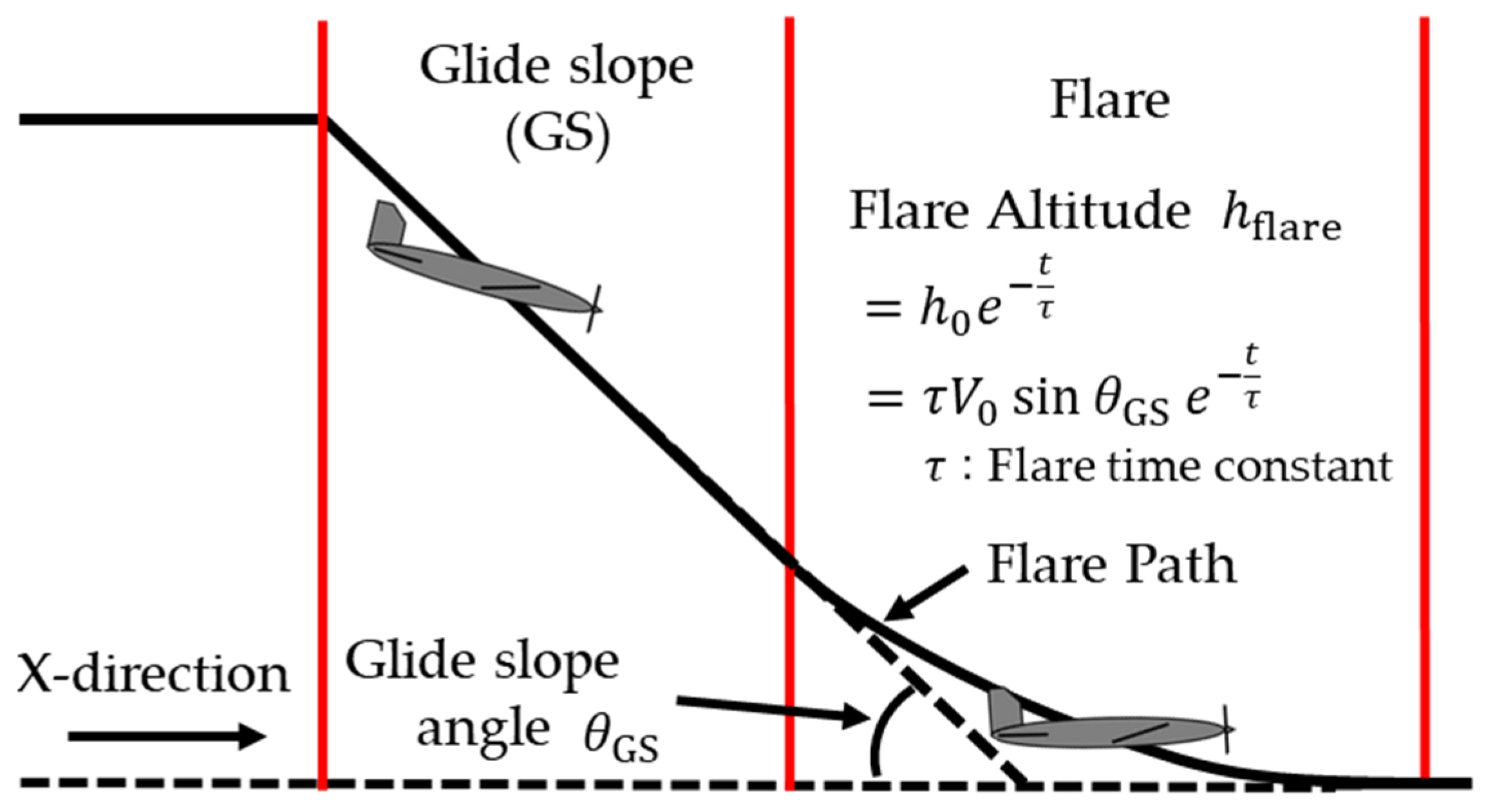
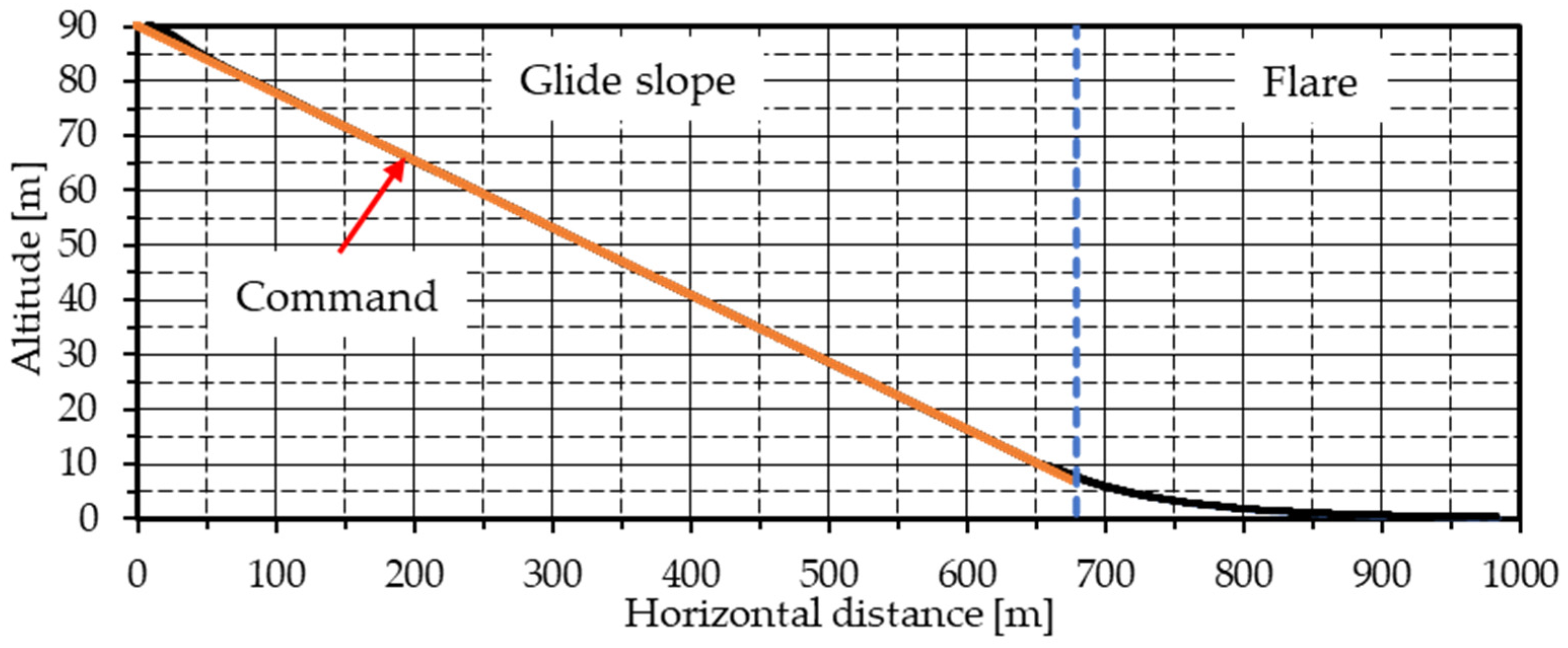
A typical landing trajectory consists of a glide slope phase, in which the airplane descends at a constant glide slope angle and airspeed, and a flare phase, in which the nose is raised to reduce the descent speed, as shown in Figure 1. The flight path of the glide slope phase is determined by the glide slope angle. Thus, the horizontal distance of the glide slope phase can be effectively shortened by increasing the glide slope angle. This approach has been well established in previous research [5,6]. Specifically, one study presents a method for calculating the maximum glide slope angle, which is determined by the stall angle of attack, using the equilibrium equation of longitudinal motion [5]. Another study presents the design and development of an autonomous flight technique for a landing trajectory that was set based on the policy of descending at the maximum glide slope angle while suppressing the forward speed [6]. All of these studies dealt with the glide slope trajectory.

The flight path during the flare phase follows an exponential function, where a greater flight path curvature results in a shorter horizontal distance during the flare phase. The parameter dominating this curvature is the flare time constant. Generally, the flare time constant is determined based on the distance between the transmitter point and the touchdown point. The method involves using an exponential function, its derivative, the glide slope angle, and the distance [7,8,9]. To our best knowledge, there are few studies that focus on short-distance landing during the flare phase. In [5], however, the focus is on short-distance landing, where a method is proposed for determining the minimum flare time constant by deriving the static relationship between the angle of attack and the flare time constant at the start of the flare phase from the equations of motion for a point mass restricted to the longitudinal plane. It is then analytically demonstrated that the flare time constant is minimum at the maximum angle of attack, in terms of airplane performance. In essence, this method uses the relationship between the angle of attack and the flare time constant at the start of the flare phase, which is derived from the equations of motion of a point mass restricted to the longitudinal plane. However, it is not necessarily the case that the maximum angle of attack, nor a value close to it, is reached at the start of the flare. In addition, it is impossible to incorporate the equation of rotational motion using the conventional method for determining the minimum flare time constant, so it is not incorporated. Therefore, in many cases, it is highly likely that an unrealizable flare time constant will be determined as a result of not meeting the assumptions of the conventional method.

In consideration of the above, in this study, we propose a new method for determining the flare time constant in which the horizontal distance of the flare phase is minimized, with the aim of reducing the aerial distance of fixed-wing UAVs. The landing distance in the flare phase is proportional to the flight speed. So, the higher the speed of the UAV, the longer the landing distance. Therefore, it is important to develop short-distance landing control techniques for high-speed UAVs that are applicable during the flare phase. Essentially, this method requires solving a nonlinear optimization problem for equations of motion, both for translational motion in the XZ plane and for rotational motion around the Y-axis under the initial conditions and terminal conditions as equality constraints. Unlike the conventional method for determining flare time constants, this method takes into account the pitch angular velocity generated by the rotational motion during the flare phase and attitude at the start of the flare phase, which cannot be considered in the conventional point mass model, by including the rotational motion. Therefore, the proposed method strictly takes into account the characteristics of the UAV and can be applied to a wide range of UAVs. In this paper, first, in Section 2, we explain both the formulation of the optimal control problem for determining the flare time constant and the numerical solution method used. In Section 3, we present the calculation results when the method shown in Section 2 is applied to the target UAV. In addition, we simulate a longitudinal flight to confirm both the validity of the motion model equation presented in Section 2 and the accuracy of the optimal solution, and we describe the results. In Section 4, we conduct a six-degrees-of-freedom flight simulation that includes sensor noise and wind disturbance to confirm whether it is possible to achieve landing control using the optimized flare time constant obtained and describe the simulation results. Finally, in Section 5, we conclude this paper.

2. Method for Determining the Flare Time Constant as an Optimal Control Problem

In this section, the optimal control problem and the numerical solution for solving the optimal control problem are described. In Section 2.1, the optimal control problem is formulated in which the flare time constant is treated as part of the state variables. In Section 2.2, the numerical solution for solving the optimal control problem defined in Section 2.1 is described. In this study, the optimal flare time constant is determined by applying the numerical solution presented in Section 2.2.

2.1. Formulation of the Optimal Control Problem

Section 2.1.1, Section 2.1.2, Section 2.1.3, Section 2.1.4 and Section 2.1.5 describe the elements that constitute the optimal control problem, including the dynamic constraints, evaluation function, boundary conditions, and inequality constraints. Finally, in Section 2.1.6, the formulation of the optimal control problem is clarified using these elements introduced in Section 2.1.1, Section 2.1.2, Section 2.1.3, Section 2.1.4 and Section 2.1.5.

2.1.1. Motion Model During Flare Flight

In this study, the motion of the UAV is expressed in a coordinate system with the Z-axis pointing upwards. Assuming that the airplane is descending along the center line of the runway at a constant roll angle of zero degrees during a flare, the lateral motion is ignored, and only the longitudinal motion is considered in the optimal control problem. The longitudinal motion consists of translational motion along the X- and Z-axes and rotational motion around the Y-axis. The external forces acting on the UAV comprise the lift ($L_{\mathrm{w}}·L_{\mathrm{t}}$) and drag D forces generated by the main wings and horizontal tail, as well as gravity $\mathrm{m}\mathrm{g}$ and thrust T, as shown in Figure 2. These external forces are resolved into the X- and Z-axes, and the equations of motion for the UAV’s translational motion are derived as Equations (1) and (2). The rotational motion is derived as Equation (3).

$$m\dot{u}=T\cos \theta -L_{\mathrm{w}}\sin \gamma -D\cos \gamma -L_{\mathrm{t}}\sin \gamma$$

(1)

$$m\ddot{h}=-mg+T\sin \theta +L_{\mathrm{w}}\cos \gamma -D\sin \gamma +L_{\mathrm{t}}\cos \gamma$$

(2)

$$I_{\mathrm{y}\mathrm{y}}\dot{q}=M_{\mathrm{w}\mathrm{i}\mathrm{n}\mathrm{g}}+M_{\mathrm{t}\mathrm{a}\mathrm{i}\mathrm{l}}+M_{\mathrm{f}\mathrm{u}\mathrm{s}\mathrm{e}\mathrm{l}\mathrm{a}\mathrm{g}\mathrm{e}}$$

(3)

Only the newly introduced variables included in Equations (1)–(3) are defined here.

$\dot{u}$ represents the horizontal acceleration in meters per second squared. $\ddot{h}$ represents the vertical acceleration in meters per second squared. $\theta$ represents the pitch angle in radians.

Only newly introduced variables included in Equation (3) are defined here.

$I_{\mathrm{y}\mathrm{y}}$ represents the moment of inertia around the pitch axis in kilogram squared meters. $\dot{q}$ represents the pitch angle acceleration in radians per second squared. $M_{\mathrm{w}\mathrm{i}\mathrm{n}\mathrm{g}}$ represents the pitching moment due to the lift of the main wings in Newton meters. $M_{\mathrm{t}\mathrm{a}\mathrm{i}\mathrm{l}}$ represents the pitching moment due to the lift of the horizontal tail in Newton meters. $M_{\mathrm{f}\mathrm{u}\mathrm{s}\mathrm{e}\mathrm{l}\mathrm{a}\mathrm{g}\mathrm{e}}$ represents the fuselage moment in Newton meters.

The lift of the main wings $L_{\mathrm{w}}$, the lift of the horizontal tail $L_{\mathrm{t}}$, and drag $D$ included in Equations (1) and (2) are expressed by Equations (4)–(7).

$$L_{\mathrm{w}}={\displaystyle \frac{1}{2}}\rho S{V}^2\left(C_{\mathrm{L}0}+C_{\mathrm{L}\mathrm{w}}\left(\alpha +i_{\mathrm{w}\mathrm{i}\mathrm{n}\mathrm{g}}\right)\right)$$

(4)

$$L_{\mathrm{t}}={\displaystyle \frac{1}{2}}\rho S_{\mathrm{t}}{V}^2\left(C_{\mathrm{L}\mathrm{t}}\alpha +C_{\mathrm{L}\mathrm{t}}{\tau }_{\mathrm{t}}\delta e+C_{\mathrm{L}\mathrm{t}}{\displaystyle \frac{q{l}_{\mathrm{t}}}{V}}\right)$$

(5)

$$D={\displaystyle \frac{1}{2}}\rho S{V}^2\left(C_{\mathrm{D}0}+{\displaystyle \frac{C_{\mathrm{L}}^2}{\pi eAR}}\right)$$

(6)

$$C_{\mathrm{L}}=C_{\mathrm{L}0}+C_{\mathrm{L}\mathrm{w}}\left(\alpha +i_{\mathrm{w}\mathrm{i}\mathrm{n}\mathrm{g}}\right)+{\displaystyle \frac{S_{\mathrm{t}}}{S}}\left(C_{\mathrm{L}\mathrm{t}}\alpha +C_{\mathrm{L}\mathrm{t}}{\tau }_{\mathrm{t}}\delta e+C_{\mathrm{L}\mathrm{t}}{\displaystyle \frac{q{l}_{\mathrm{t}}}{V}}\right)$$

(7)

Only newly introduced variables included in Equations (4)–(7) are defined here.

$S$ represents the wing area in square meters. $S_{\mathrm{t}}$ represents the horizontal tail area in square meters. $V$ represents the airspeed in meters per second. $C_{\mathrm{L}0}$ represents the coefficient of lift in a dimensionless form. $C_{\mathrm{L}\mathrm{w}}$ represents the lift of the main wings per unit of the angle of attack per radian. $C_{\mathrm{L}\mathrm{t}}$ represents the lift of the horizontal tail per unit of the angle of attack per radian. $i_{\mathrm{w}\mathrm{i}\mathrm{n}\mathrm{g}}$ represents the main wing-mounting angle in radians. ${\tau }_{\mathrm{t}}$ represents the elevator time constant in a dimensionless form. $\delta e$ represents the elevator angle in radians. $q$ represents the pitch angular velocity in radians per second. $C_{\mathrm{D}0}$ represents the parasitic drag coefficient in a dimensionless form. $e$ represents the airplane efficiency in a dimensionless form. $AR$ represents the aspect ratio in a dimensionless form. $C_{\mathrm{L}}$ represents the airplane lift coefficient in a dimensionless form.

The pitching moment due to the lift of the main wings $M_{\mathrm{w}\mathrm{i}\mathrm{n}\mathrm{g}}$, the pitching moment due to the lift of the horizontal tail $M_{\mathrm{t}\mathrm{a}\mathrm{i}\mathrm{l}}$, and the fuselage moment $M_{\mathrm{f}\mathrm{u}\mathrm{s}\mathrm{e}\mathrm{l}\mathrm{a}\mathrm{g}\mathrm{e}}$ included in Equation (3) are expressed by Equations (8)–(10).

$$M_{\mathrm{w}\mathrm{i}\mathrm{n}\mathrm{g}}={\displaystyle \frac{1}{2}}\rho V^{2}Sc{C}_{\mathrm{m}0}+L_{\mathrm{w}}\cos \alpha \left(h_{\mathrm{c}\mathrm{g}}-h_{\mathrm{a}\mathrm{c}}\right)c$$

(8)

$$M_{\mathrm{t}\mathrm{a}\mathrm{i}\mathrm{l}}=-L_{\mathrm{t}}\cos \alpha l_{\mathrm{t}}$$

(9)

$$M_{\mathrm{f}\mathrm{u}\mathrm{s}\mathrm{e}\mathrm{l}\mathrm{a}\mathrm{g}\mathrm{e}}={\displaystyle \frac{1}{2}}\rho V^2{V}_{\mathrm{f}\mathrm{u}\mathrm{s}}\left(2\alpha \right)$$

(10)

Only newly introduced variables included in Equations (8)–(10) are defined here.

$V_{\mathrm{f}\mathrm{u}\mathrm{s}}$ represents the fuselage volume in cubic meters.

2.1.2. Dynamic Constraints of the Optimal Control Problem

The state variables $\mathit{x}\left(t\right)$ of the optimal control problem are the horizontal distance $x\left(t\right)$, altitude $h\left(t\right)$, horizontal velocity $u\left(t\right)$, vertical velocity $\dot{h}\left(t\right)$, flare time constant $\tau \left(t\right)$, pitch angle $\theta \left(t\right)$, and pitch angular velocity $q\left(t\right)$, and the control variable $\mathit{u}\left(t\right)$ of the optimal control problem is the elevator angle $\delta e\left(t\right)$. The state variables and control variable are expressed as Equation (11).

$$\begin{array}{c}\mathit{x}\left(t\right)={\left[\begin{array}{ccccccc}x\left(t\right)& h\left(t\right)& u\left(t\right)& \dot{h}\left(t\right)& \tau \left(t\right)& \theta \left(t\right)& q\left(t\right)\end{array}\right]}^{\mathrm{T}}\mathit{u}(t)=\delta e(t)\\ t\in \left[t_0,t_{\mathrm{f}}\right]\end{array}$$

(11)

The state equation is derived from the equations of translational and rotational motion (1) to (3) and the relationship that the flare time constant remains constant. The state equation is expressed as Equation (12a), and functions as a dynamic constraint in formulating the optimal control problem. The path angle $\gamma \left(t\right)$, the angle of attack $\alpha \left(t\right)$, the airspeed $V\left(t\right)$, the lift of the main wings $L_{\mathrm{w}}\left(t\right)$, the lift of the horizontal tail $L_{\mathrm{t}}\left(t\right)$, drag $D\left(t\right)$, the airplane lift coefficient $C_{\mathrm{L}}\left(t\right)$, the pitching moment due to the lift of the main wings $M_{\mathrm{w}\mathrm{i}\mathrm{n}\mathrm{g}}\left(t\right)$, the pitching moment due to the lift of the horizontal tail $M_{\mathrm{t}\mathrm{a}\mathrm{i}\mathrm{l}}\left(t\right)$, and the fuselage moment $M_{\mathrm{f}\mathrm{u}\mathrm{s}\mathrm{e}\mathrm{l}\mathrm{a}\mathrm{g}\mathrm{e}}\left(t\right)$ included in the state equation are expressed in Equations (12b)–(12k), respectively, and the state variables and control variable defined in Equation (11) are used, respectively.

$$\dot{\mathit{x}}(t)=\left[\begin{array}{c}\dot{x}\left(t\right)\\ \dot{h}\left(t\right)\\ \dot{u}\left(t\right)\\ \ddot{h}\left(t\right)\\ \dot{\tau }\left(t\right)\\ \dot{\theta }\left(t\right)\\ \dot{q}\left(t\right)\end{array}\right]=\left[\begin{array}{c}u\left(t\right)\\ \dot{h}\left(t\right)\\ \left(T\cos \theta \left(t\right)-L_{\mathrm{w}}\left(t\right)\sin \gamma \left(t\right)-D\left(t\right)\cos \gamma \left(t\right)-L_{\mathrm{t}}\left(t\right)\sin \gamma \left(t\right)\right){\displaystyle \frac{1}{m}}\\ \left(mg-T\sin \theta \left(t\right)-L_{\mathrm{w}}\left(t\right)\cos \gamma \left(t\right)+D\left(t\right)\sin \gamma \left(t\right)-L_{\mathrm{t}}\left(t\right)\cos \gamma \left(t\right)\right){\displaystyle \frac{1}{m}}\\ 0.0\\ q\left(t\right)\\ \left(M_{\mathrm{w}\mathrm{i}\mathrm{n}\mathrm{g}}\left(t\right)+M_{\mathrm{t}\mathrm{a}\mathrm{i}\mathrm{l}}\left(t\right)+M_{\mathrm{f}\mathrm{u}\mathrm{s}\mathrm{e}\mathrm{l}\mathrm{a}\mathrm{g}\mathrm{e}}\left(t\right)\right)/I_{\mathrm{y}\mathrm{y}}\end{array}\right]$$

(12a)

$$\gamma (t)={\tan }^{-1}{\displaystyle \frac{\dot{h}\left(t\right)}{u\left(t\right)}}$$

(12b)

$$\alpha \left(t\right)=\theta \left(t\right)-\gamma \left(t\right)$$

(12c)

$$V(t)=\sqrt{{u\left(t\right)}^2+{\dot{h}\left(t\right)}^2}$$

(12d)

$$L_{\mathrm{w}}(t)={\displaystyle \frac{1}{2}}\rho S{V\left(t\right)}^2\left(C_{\mathrm{L}0}+C_{\mathrm{L}\mathrm{w}}\left(\alpha \left(t\right)+i_{\mathrm{w}\mathrm{i}\mathrm{n}\mathrm{g}}\right)\right)$$

(12e)

$$L_{\mathrm{t}}(t)={\displaystyle \frac{1}{2}}\rho S_{\mathrm{t}}{V\left(t\right)}^2\left(C_{\mathrm{L}\mathrm{t}}\alpha (t)+C_{\mathrm{L}\mathrm{t}}{\tau }_{\mathrm{t}}\delta e(t)+C_{\mathrm{L}\mathrm{t}}{\displaystyle \frac{q\left(t\right)l_{\mathrm{t}}}{V\left(t\right)}}\right)$$

(12f)

$$C_{\mathrm{L}}(t)=C_{\mathrm{L}0}+C_{\mathrm{L}\mathrm{w}}\left(\alpha \left(t\right)+i_{\mathrm{w}\mathrm{i}\mathrm{n}\mathrm{g}}\right)+{\displaystyle \frac{S_{\mathrm{t}}}{S}}\left(C_{\mathrm{L}\mathrm{t}}\alpha (t)+C_{\mathrm{L}\mathrm{t}}{\tau }_{\mathrm{t}}\delta e(t)+C_{\mathrm{L}\mathrm{t}}{\displaystyle \frac{q\left(t\right)l_{\mathrm{t}}}{V\left(t\right)}}\right)$$

(12g)

$$D(t)={\displaystyle \frac{1}{2}}\rho S{V\left(t\right)}^2\left(C_{\mathrm{D}0}+{\displaystyle \frac{{C_{\mathrm{L}}\left(t\right)}^2}{\pi eAR}}\right)$$

(12h)

$$M_{\mathrm{w}\mathrm{i}\mathrm{n}\mathrm{g}}(t)={\displaystyle \frac{1}{2}}\rho {V\left(t\right)}^{2}Sc{C}_{\mathrm{m}0}+L_{\mathrm{w}}(t)\cos \alpha (t)\left(h_{\mathrm{c}\mathrm{g}}-h_{\mathrm{a}\mathrm{c}}\right)c$$

(12i)

$$M_{\mathrm{t}\mathrm{a}\mathrm{i}\mathrm{l}}\left(t\right)=-L_{\mathrm{t}}\left(t\right)\cos \alpha \left(t\right)l_{\mathrm{t}}$$

(12j)

$$M_{\mathrm{f}\mathrm{u}\mathrm{s}\mathrm{e}\mathrm{l}\mathrm{a}\mathrm{g}\mathrm{e}}(t)={\displaystyle \frac{1}{2}}\rho {V\left(t\right)}^2{V}_{\mathrm{f}\mathrm{u}\mathrm{s}}\left(2\alpha \left(t\right)\right)$$

(12k)

Only newly introduced variables included in Equations (11)–(12) are defined here.

$t_0$ represents the initial time in seconds. $t_{\mathrm{f}}$ represents the terminal time in seconds. $\dot{x}$ represents the horizontal velocity in meters per second. $\dot{\theta }$ represents the pitch angular velocity in radians per second.

2.1.3. Evaluation Function

Here, we set two evaluation indices and minimize the weighted sum of these indices. The first is the index aimed at achieving the ideal exponential-type path during the flare path. The second is the index aimed at minimizing the horizontal distance during the flare path. From these, the evaluation function J used in the optimal control problem is expressed as Equation (13). A and B are the weight coefficients for each index of the evaluation function, and both are positive. Here, the non-negativity of the two terms of the evaluation function is demonstrated below. The first term is the product of the sum of the squares of the deviations and the weighting coefficient A, so it is clearly non-negative. The second term, which is the product of the terminal horizontal distance $x_{\mathrm{f}} (\mathrm{o}\mathrm{r} x(t_{\mathrm{f}}\left)\right)$ and the weighting coefficient B, is clearly physically non-negative so long as the UAV flies heading in the direction of the landing point. In addition, the weight coefficients of the evaluation function are determined heuristically based on the following two criteria:

• Emphasis on achieving the ideal path for the flare phase;

To prioritize achieving the ideal flare path, represented by the first term of the evaluation function, coefficient A was set sufficiently large to enhance its influence.

2.

Ensuring optimization convergence and physical feasibility.

The weight coefficients were adjusted to ensure that the optimization calculation converges properly and that the obtained optimal solution remains physically feasible.

$$J=\mathrm{A}{\int }_{t_0}^{t_{\mathrm{f}}}{\left(h(t)-\tau (t)V_0\sin {\theta }_{\mathrm{G}\mathrm{S}}{e}^{-{\displaystyle \frac{t}{\tau \left(t\right)}}}\right)}^{2}dt+\mathrm{B}x(t_{\mathrm{f}})$$

(13)

The first term of Equation (13) represents the sum of the squared deviation between the approximate flare path, determined from Equation (14), and the altitude. The second term in Equation (13) indicates the x-component of the position at the final time.

$$h_{\mathrm{f}\mathrm{l}\mathrm{a}\mathrm{r}\mathrm{e}}(t)=h_0{e}^{-{\displaystyle \frac{t}{\tau }}}=\tau V_0\sin {\theta }_{\mathrm{G}\mathrm{S}}{e}^{-{\displaystyle \frac{t}{\tau }}}$$

(14)

2.1.4. Initial and Terminal Conditions and Thrust During Flare Flight

The flight conditions at the start of the flare (terminal of the glide slope) are set as the initial conditions. The initial horizontal velocity $u_0 (\mathrm{o}\mathrm{r} u(t_0\left)\right)$, vertical velocity ${\dot{h}}_0 (\mathrm{o}\mathrm{r} \dot{h}(t_0\left)\right)$, and altitude $h_0 (\mathrm{o}\mathrm{r} h(t_0\left)\right)$ are determined based on Equations (15)–(17) by using the initial flare time constant ${\tau }_0 (\mathrm{o}\mathrm{r} \tau (t_0\left)\right), V_0,\mathrm{a}\mathrm{n}\mathrm{d} {\theta }_{\mathrm{G}\mathrm{S}}$. In Equation (17), used for calculating the initial altitude, $h_0$ is derived based on Equation (18), which is derived by differentiating Equation (14).

$$u_0=u\left(t_0\right)=V_0\cos {\theta }_{\mathrm{G}\mathrm{S}}$$

(15)

$${\dot{h}}_0=\dot{h}(t_0)=V_0\sin {\theta }_{\mathrm{G}\mathrm{S}}$$

(16)

$$h_0=h\left(t_0\right)={\tau }_0\left|{\dot{h}}_0\right|={\tau }_0{V}_0\sin \left(-{\theta }_{\mathrm{G}\mathrm{S}}\right)$$

(17)

$${\dot{h}}_{\mathrm{f}\mathrm{l}\mathrm{a}\mathrm{r}\mathrm{e}}(t)=-{\displaystyle \frac{h_{\mathrm{f}\mathrm{l}\mathrm{a}\mathrm{r}\mathrm{e}}\left(t\right)}{\tau }}$$

(18)

The initial altitude $h_0$ is a variable in the process of deriving the optimal solution because the initial flare time constant ${\tau }_0$ is a variable. The initial pitch angle ${\theta }_0 (\mathrm{o}\mathrm{r} \theta (t_0\left)\right)$ is derived from the balance in the glide slope and calculated using the initial angle of attack ${\alpha }_0$. The ${\alpha }_0$ is calculated by solving the longitudinal equilibrium equation with the left side of Equations (1)–(3) set to zero and using the predetermined glide slope angle ${\theta }_{\mathrm{G}\mathrm{S}}$. ${\theta }_0$ is expressed in Equation (19).

$${\theta }_0=\theta \left(t_0\right)={\alpha }_0+\left(-{\theta }_{\mathrm{G}\mathrm{S}}\right)$$

(19)

The initial horizontal position $x_0(\mathrm{o}\mathrm{r} x(t_0\left)\right)$ and the pitch angular velocity $q_0(\mathrm{o}\mathrm{r} q(t_0\left)\right)$ are set to zero. The initial flare time constant ${\tau }_0$ and the elevator angle ${\delta e}_0(\mathrm{o}\mathrm{r} \delta e(t_0\left)\right)$ are not constrained and are determined based on the converged solutions. In addition, the balanced thrust during the glideslope phase $T_0$ is simultaneously calculated by solving the equilibrium equation, and it is assumed that the thrust during the flare phase is a constant at $T_0$.

The terminal conditions are determined from the flight condition at touchdown. Regarding the terminal altitude $h_{\mathrm{f}} (\mathrm{o}\mathrm{r} h(t_{\mathrm{f}}\left)\right)$, the height of the UAV’s landing gear $h_{\mathrm{g}\mathrm{e}\mathrm{a}\mathrm{r}}$ has been taken into consideration. The terminal vertical velocity $\dot{h_{\mathrm{f}}} (\mathrm{o}\mathrm{r} \dot{h}(t_{\mathrm{f}}\left)\right)$ is derived by substituting the terminal altitude $h_{\mathrm{f}}$ and the flare time constant ${\tau }_{\mathrm{f}} (\mathrm{o}\mathrm{r} \tau (t_{\mathrm{f}}\left)\right)$ into Equation (18). The terminal horizontal position $x_{\mathrm{f}}(\mathrm{o}\mathrm{r} x(t_{\mathrm{f}}\left)\right)$, horizontal velocity $u_{\mathrm{f}} (\mathrm{o}\mathrm{r} u(t_{\mathrm{f}}\left)\right)$, flare time constant ${\tau }_{\mathrm{f}}$, pitch angle ${\theta }_{\mathrm{f}} (\mathrm{o}\mathrm{r} \theta (t_{\mathrm{f}}\left)\right)$, pitch angular velocity $q_{\mathrm{f}}(\mathrm{o}\mathrm{r} q(t_{\mathrm{f}}\left)\right)$, and elevator angle ${\delta e}_{\mathrm{f}}(\mathrm{o}\mathrm{r} \delta e(t_{\mathrm{f}}\left)\right)$ are not constrained and are determined based on the converged solutions.

Therefore, the boundary conditions (the initial conditions $\mathit{x}\left(t_0\right)$ and the terminal conditions $\mathit{x}\left(t_{\mathrm{f}}\right)$) are expressed as Equation (20). Part of the boundary conditions ($h\left(t_0\right),\tau \left(t_0\right),x\left(t_{\mathrm{f}}\right),u\left(t_{\mathrm{f}}\right),\dot{h}\left(t_{\mathrm{f}}\right),\tau \left(t_{\mathrm{f}}\right),\theta \left(t_{\mathrm{f}}\right), \mathrm{a}\mathrm{n}\mathrm{d} q\left(t_{\mathrm{f}}\right)$) are formulated as “free”. When solving optimal control problems using direct methods, the unconstrained boundary conditions are treated as discretized optimization variables, and the transversality conditions are implicitly satisfied.

$$\mathit{x}\left(t_0\right)=\left[\begin{array}{c}x\left(t_0\right)\\ h\left(t_0\right)\\ u\left(t_0\right)\\ \dot{h}\left(t_0\right)\\ \tau \left(t_0\right)\\ \theta \left(t_0\right)\\ q\left(t_0\right)\end{array}\right]=\left[\begin{array}{c}0.0\\ \tau \left(t_0\right)V_0\sin \left(-{\theta }_{\mathrm{G}\mathrm{S}}\right)\left(\mathrm{f}\mathrm{r}\mathrm{e}\mathrm{e}\right)\\ V_0\cos {\theta }_{\mathrm{G}\mathrm{S}}\\ V_0\sin {\theta }_{\mathrm{G}\mathrm{S}}\\ \mathrm{f}\mathrm{r}\mathrm{e}\mathrm{e}\\ {\alpha }_0+\left(-{\theta }_{\mathrm{G}\mathrm{S}}\right)\\ 0.0\end{array}\right] \mathit{x}\left(t_{\mathrm{f}}\right)=\left[\begin{array}{c}x\left(t_{\mathrm{f}}\right)\\ h\left(t_{\mathrm{f}}\right)\\ u\left(t_{\mathrm{f}}\right)\\ \dot{h}\left(t_{\mathrm{f}}\right)\\ \tau \left(t_{\mathrm{f}}\right)\\ \theta \left(t_{\mathrm{f}}\right)\\ q\left(t_{\mathrm{f}}\right)\end{array}\right]=\left[\begin{array}{c}\mathrm{f}\mathrm{r}\mathrm{e}\mathrm{e}\\ h_{\mathrm{g}\mathrm{e}\mathrm{a}\mathrm{r}}\\ \mathrm{f}\mathrm{r}\mathrm{e}\mathrm{e}\\ -h_{\mathrm{g}\mathrm{e}\mathrm{a}\mathrm{r}}/\tau \left(t_{\mathrm{f}}\right) \left(\mathrm{f}\mathrm{r}\mathrm{e}\mathrm{e}\right)\\ \mathrm{f}\mathrm{r}\mathrm{e}\mathrm{e}\\ \mathrm{f}\mathrm{r}\mathrm{e}\mathrm{e}\\ \mathrm{f}\mathrm{r}\mathrm{e}\mathrm{e}\end{array}\right]$$

(20)

2.1.5. Inequality Constraints

The inequality constraints are defined for the angle of attack $\alpha$, elevator angle $\delta e$, and pitch angular velocity $q$. The angle of attack $\alpha$, is constrained within the stall angle of attack ${\alpha }_{\mathrm{s}\mathrm{t}\mathrm{a}\mathrm{l}\mathrm{l}}$. The motion of the elevator angle $\delta e$ is constrained within the maximum allowable angle range ${\delta e}_{\mathrm{m}\mathrm{a}\mathrm{x}}$. The pitch angular velocity $q$ is set to be constrained by the maximum pitch angular velocity $q_{\mathrm{l}\mathrm{i}\mathrm{m}\mathrm{i}\mathrm{t}}$ that can occur during steady-state flight during a flare phase. It is expressed as Equation (21), which uses the difference $∆\theta$ between the initial pitch angle ${\theta }_0$ and zero degrees of pitch angle, together with the time $∆t$ required to raise the nose from the initial pitch angle ${\theta }_0$ to zero degrees of pitch angle. The time $∆t$ is the settling time of the step response of the pitch angle control system. The settling time $t_{\mathrm{s}\_\mathrm{p}\mathrm{i}\mathrm{t}\mathrm{c}\mathrm{h}}$ is the time required for the output to fall within $\pm 5\%$ of the target value.

$$q_{\mathrm{l}\mathrm{i}\mathrm{m}\mathrm{i}\mathrm{t}}={\displaystyle \frac{∆\theta }{∆t}}={\displaystyle \frac{0.0-{\theta }_0}{t_{{\mathrm{s}}_{\_\mathrm{p}\mathrm{i}\mathrm{t}\mathrm{c}\mathrm{h}}}}}$$

(21)

Thus, the inequality constraints for the pitch angular velocity are $-q_{\mathrm{l}\mathrm{i}\mathrm{m}\mathrm{i}\mathrm{t}}\le q\le q_{\mathrm{l}\mathrm{i}\mathrm{m}\mathrm{i}\mathrm{t}}$.

Therefore, the inequality constraints $\mathit{g}\left(\mathit{x},\mathit{u},t\right)$ are expressed as Equation (22).

$$\mathit{g}\left(\mathit{x},\mathit{u},t\right)=\left[\begin{array}{c}-{\delta e}_{\mathrm{m}\mathrm{a}\mathrm{x}}-\delta e\left(t\right)\\ \delta e\left(t\right)-{\delta e}_{\mathrm{m}\mathrm{a}\mathrm{x}}\\ -{\alpha }_{\mathrm{s}\mathrm{t}\mathrm{a}\mathrm{l}\mathrm{l}}-\alpha \left(t\right)\\ \alpha \left(t\right)-{\alpha }_{\mathrm{s}\mathrm{t}\mathrm{a}\mathrm{l}\mathrm{l}}\\ -q_{\mathrm{l}\mathrm{i}\mathrm{m}\mathrm{i}\mathrm{t}}-q\left(t\right)\\ q\left(t\right)-q_{\mathrm{l}\mathrm{i}\mathrm{m}\mathrm{i}\mathrm{t}}\end{array}\right]\le \mathbf{0}$$

(22)

2.1.6. Clarification of the Optimal Control Problem

The optimal control problem consists of dynamic constraints, an evaluation function, boundary conditions, and inequality constraints.

The state and control variables are expressed in Equation (11), as defined in Section 2.1.2. These variables are associated with the translational and rotational motion in the longitudinal direction. The dynamic constraints are expressed in Equation (12a), as defined in Section 2.1.2. By incorporating the UAV’s longitudinal equations of motion as dynamic constraints, the optimal flare time constant can be determined as a value achievable by the UAV. As defined in Section 2.1.3, Section 2.1.4 and Section 2.1.5, the evaluation function, boundary conditions, and inequality constraints are expressed in Equations (13), (20), and (22), respectively.

2.2. Numerical Solution of Optimal Control Problems

There are two methods for numerically solving optimal control problems: the indirect method and the direct method. Unlike the former, the latter enables state space inequality constraints without using special transformations, such as the slack variable method or the time axis folding method [10], and it is highly robust in finding the optimal solution [11]. For this reason, we use the Hermite–Simpson collocation method, which is classified as a direct method. It divides the time domain into equally spaced nodes and uses a third-order Hermite interpolation polynomial to interpolate state variables at the collocation points, which are located at the midpoints of the nodes. Control variables are interpolated linearly [12]. Using this method, we discretize the optimal control problem and convert it into a nonlinear optimization problem. In this study, sequential quadratic programming (SQP) is employed as a method for solving nonlinear optimization problems. The rationale for its adoption is described below.

Methods for solving nonlinear optimization problems are broadly categorized into global optimization methods and local optimization methods. Global methods include genetic algorithms (GAs) and particle swarm optimization (PSO). A GA mimics the evolutionary process of biological organisms by selecting and evolving highly fit individuals [13]. PSO defines each particle as a candidate solution in the search space and updates its state based on a combination of the particle’s own best position, the global best position, and velocity updates [14]. These algorithms offer advantages such as requiring no gradient information, being robust against multimodal functions, and providing the potential to locate global optima [13,14]. However, they also face limitations. A GA may suffer from slow convergence or poor-quality solutions depending on the initial population, and early convergence remains a common issue [13]. PSO, originally designed for continuous variables, requires methodological extensions to handle discrete variables effectively [14].

On the other hand, local optimization methods include not only SQP but also interior point methods, with the primal–dual interior point method being particularly prevalent. This method approaches the optimal solution by following a central path within the feasible region, aiming to satisfy the Karush–Kuhn–Tucker (KKT) conditions [15]. It is well-suited to high-dimensional and sparse problems [15]. Nonetheless, challenges remain, such as reduced accuracy near the constraint boundaries due to the barrier term and the requirement for the initial point to lie strictly within the feasible region [15].

Given that this study addresses a discretized, small-scale nonlinear optimization problem that requires high solution accuracy and computational efficiency, SQP, as a representative local optimization method, is considered the most appropriate choice [16]. SQP achieves fast local convergence and high solution precision by sequentially solving quadratic programming subproblems derived from a second-order approximation of the Lagrangian and a linearization of the constraints [16]. Furthermore, it has a proven track record in various applications across engineering and scientific domains [17,18,19,20]. In addition, this study used the external Python library “Scipy” to solve the problem using sequential quadratic programming [21]. “Python” of version used in this study was 3.12.4, and “Scipy” of version was 1.13.1.

3. Method Application

The method explained in Section 2 is applied to the target airplane shown in Section 3.1. The initial and terminal conditions, thrust values, inequality constraints, and weight coefficients for the evaluation function are described in Section 3.2. The nonlinear optimization problem is solved using the conditions shown in Section 3.2, and the calculation results, including the flare time constant, are described in Section 3.3. The accuracy of the optimal solution obtained in Section 3.3 and the validity of the motion model used in the nonlinear optimization problem are confirmed in Section 3.4.

3.1. Target UAV

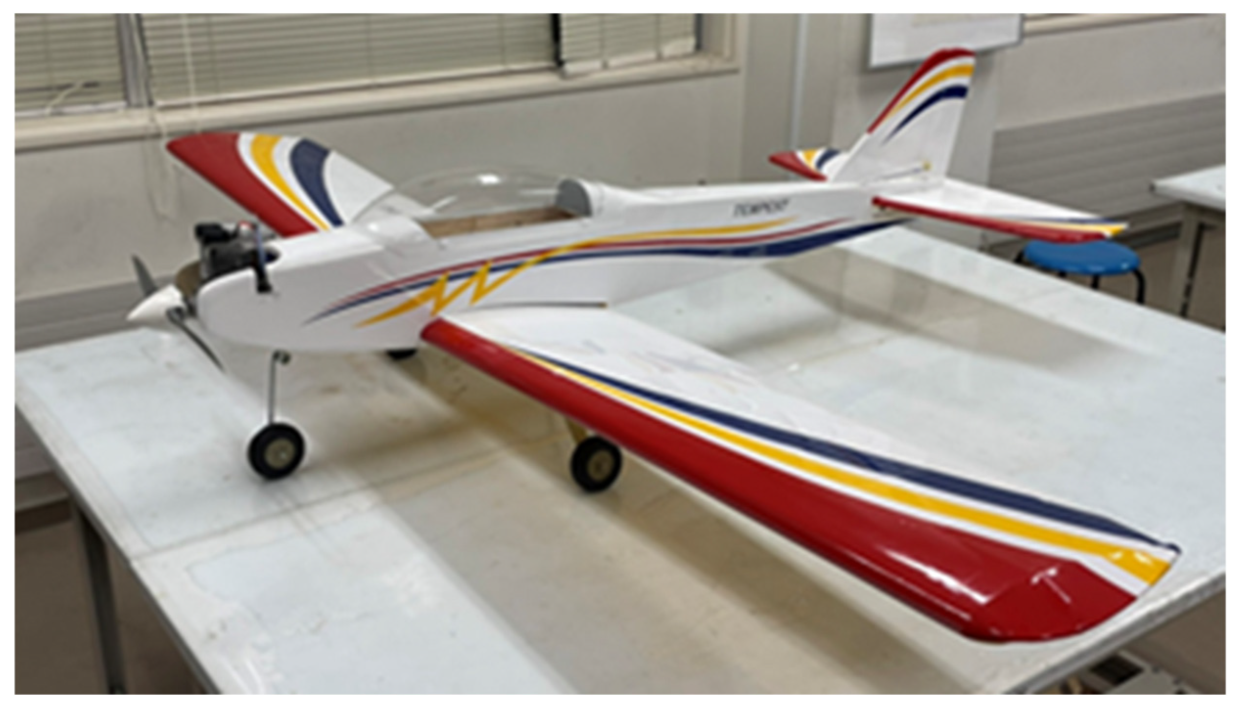
The validity of the method was confirmed using the target UAV model shown in Figure 3. This target UAV includes a propeller engine and is a low-wing, front-wheel-drive UAV equipped with a guidance control circuit and various sensors (air data sensor (ADS), inertial navigation system (INS), and pressure altitude sensor). The specifications for this UAV are summarized in

Table 1. Specifications of the target UAV.

UAV Specification	Value
m	5.7 kg
c	$0.315 \mathrm{m}$
${\mathsf{\alpha }}_{\mathrm{s}\mathrm{t}\mathrm{a}\mathrm{l}\mathrm{l}}$	10 deg.
$S$	$0.649 {\mathrm{m}}^2$
$S_{\mathrm{t}}$	$0.154 {\mathrm{m}}^2$
$e$	$0.6$
$AR$	6.54
$h_{\mathrm{c}\mathrm{g}}$	0.368
$h_{\mathrm{a}\mathrm{c}}$	0.25
$C_{\mathrm{L}\mathrm{w}}$	$3.811 1/\mathrm{r}\mathrm{a}\mathrm{d}$
$C_{\mathrm{L}\mathrm{t}}$	$3.644 1/\mathrm{r}\mathrm{a}\mathrm{d}$
${\tau }_{\mathrm{t}}$	0.5
$l_{\mathrm{t}}$	0.889
$V_{\mathrm{f}\mathrm{u}\mathrm{s}}$	0.018
$i_{\mathrm{w}\mathrm{i}\mathrm{n}\mathrm{g}}$	2.77 deg.
$h_{\mathrm{g}\mathrm{e}\mathrm{a}\mathrm{r}}$	0.2 m
${\delta e}_{\mathrm{m}\mathrm{a}\mathrm{x}}$	15.0 deg.

. Non-dimensional aerodynamic coefficients of the target UAV are required for the 6-DOF flight simulation described in the section. The non-dimensional aerodynamic coefficients were calculated using the estimation equation in [22]. The non-dimensional aerodynamic coefficients calculated using the dimensions of the target UAV shown in Table 1 are summarized in

Table 2. Aerodynamic parameters of the target UAV.

Longitudinal		Lateral
$C_{\mathrm{L}\mathsf{\alpha }}$	4.355	${C_y}_{\beta }$	−0.1623
$C_{\mathrm{L}0}$	$0.176$	${C_y}_p$	−0.03861
$C_{\mathrm{D}0}$	$0.0488$	${C_y}_{{\delta }_r}$	0.08116
$C_{\mathrm{m}0}$	−0.02411	${C_y}_r$	0.1431
${C_x}_u$	−0.08276	${C_l}_{\beta }$	−0.05330
${C_x}_{\alpha }$	0.05661	${C_l}_{{\delta }_a}$	−0.4022
${C_z}_u$	0	${C_l}_{{\delta }_r}$	0.009653
${C_z}_{\alpha }$	−4.355	${C_l}_p$	−0.7798
${C_z}_{{\delta }_e}$	−0.4324	${C_l}_r$	0.08940
${C_z}_q$	−4.881	${C_n}_{\beta }$	0.04465
${C_m}_u$	0	${C_n}_{{\delta }_a}$	0
${C_m}_{\alpha }$	−0.9096	${C_n}_{{\delta }_r}$	−0.03578
${C_m}_{{\delta }_e}$	−1.220	${C_n}_p$	−0.01062
${C_m}_q$	−13.78	${C_n}_r$	−0.1052
${C_m}_{\dot{\alpha }}$	−5.111

.

3.2. Determination of the Optimal Control Problem

The initial values of $h_0, u_0, \mathrm{a}\mathrm{n}\mathrm{d}{\dot{h}}_0$ for the optimal control problem are calculated using Equations (15)–(17) in Section 2, and the values are summarized in Table 1, including the glide slope angle ${\theta }_{\mathrm{G}\mathrm{S}}$ and the airspeed $V_0$ during the glide slope. The glide slope angle ${\theta }_{\mathrm{G}\mathrm{S}}$ is 7.0 degrees, and the airspeed $V_0$ during the glide slope is set as 25.0 m/s. The initial value of ${\theta }_0$ is calculated using Equation (19) in Section 2, and the initial value of the angle of attack ${\alpha }_0$, which is a variable in Equation (19), is calculated from the longitudinal equilibrium equation. All initial values are summarized in

Table 3. Initial values for the optimal control problem.

State and Control Variables	Value
$x_0$	0.0
$h_0$	${{\tau }_{0}V}_0\sin \left(-{\theta }_{\mathrm{G}\mathrm{S}}\right)$
$u_0$	24.8 m/s
${\dot{h}}_0$	−3.05 m/s
${\tau }_0$	free
${\theta }_0$	−9.07 deg.
$q_0$	0.0 deg./s
${\delta e}_0$	free

. The word “free” in Table 3 means “not constrained”. By solving the longitudinal equilibrium equation, the elevator angle and thrust are calculated in addition to the angle of attack, and these values are summarized in

Table 4. Solution of the equilibrium equation.

Variables	Value
${\alpha }_0$	−2.07 deg.
$T_0$	6.35 N
${\delta e}_0$	3.95 deg.

. The magnitude of thrust in the optimal control problem is assumed to be constant at 6.35 N, as per Table 4.

The terminal values for the optimal control problem are calculated based on the method in Section 3 and are shown in

Table 5. Terminal values for the optimal control problem.

State and Control Variables	Value
$x_{\mathrm{f}}$	free
$h_{\mathrm{f}}$	$0.2$
$u_{\mathrm{f}}$	free
${\dot{h}}_{\mathrm{f}}$	$-0.2/{\tau }_{\mathrm{f}}$
${\tau }_{\mathrm{f}}$	free
${\theta }_{\mathrm{f}}$	free
$q_{\mathrm{f}}$	free
${\delta e}_{\mathrm{f}}$	free

. The word “free” in Table 5 means “not constrained”.

The inequality constraints for the angle of attack $\alpha$ and the elevator angle $\delta e$ in the optimal control problem are summarized in

Table 6. Inequality constraints for the optimal control problem.

Variables	Value
$\alpha$	$-10.0\le \alpha \le 10.0 \mathrm{d}\mathrm{e}\mathrm{g}.$
$\delta e$	$-15.0\le \delta e\le 15.0 \mathrm{d}\mathrm{e}\mathrm{g}.$
$q$	$-3.8\le q\le 3.8 \mathrm{d}\mathrm{e}\mathrm{g}./\mathrm{s}$

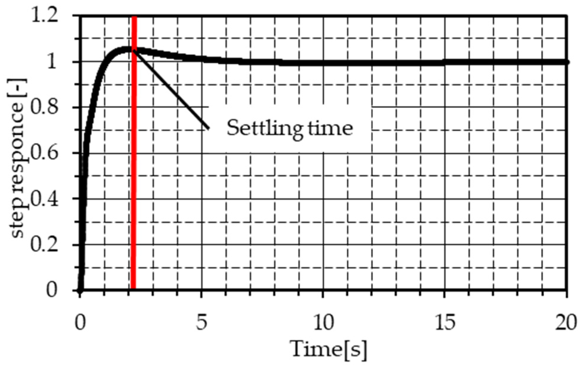
. The inequality constraints for the pitch angular velocity $q$ is calculated using Equation (21) in Section 2. $∆\theta$ is calculated as −9.07 degrees from Table 3. $∆t$ is determined by the settling time of the step response of the pitch angle control system, which is the flight control system during landing, as shown in Section 5. The step response of the pitch angle control system is shown in Figure 4, and the settling time is confirmed as 2.37 s because the settling time in this study is defined as the time it takes to converge to $\pm 5\%$ or less of the target value. As a result, the upper limit of the pitch angular velocity is determined, as summarized in Table 6.

The weight coefficients A and B in the evaluation function, and the number of nodes N when converting from the optimal control problem to the nonlinear optimization problem are summarized in

Table 7. Weighting factor and number of nodes.

Variable	Value
A	1.2
$\mathrm{B}$	0.05
$\mathrm{N}$	100

.

3.3. Results for Determination of the Flare Time Constants

The optimal control problem is converted into a nonlinear optimization problem using Hermite–Simpson collocation and is numerically solved by the sequential quadratic programming (SQP) method using the conditions summarized in Table 1, Table 2, Table 3, Table 4, Table 5, Table 6 and Table 7. When solving with the proposed method, an initial solution is required. In this study, the sequential quadratic programming method is not sensitive to initial solutions and consistently converges to nearly the same solution when moderate and reasonable initial solutions are provided. In this study, various initial solutions were set, and the nonlinear optimization problem was solved, respectively. Specifically, the initial solution of the flare time constant is constant and given within the range of 1.3 to 2.5 s. The initial solutions of altitude and descent rate are determined using Equations (14) and (18), respectively, and vary depending on the initial solution of the flare time constant. The initial solutions of horizontal distance and horizontal velocity are computed based on an airspeed of 25 m/s, the time t, and the corresponding initial solution of descent rate. The initial solution of the pitch angle is adjusted to ensure that the nose is raised while satisfying the inequality constraint on pitch angular velocity, and the initial solution of the elevator deflection angle is set to a constant negative value.

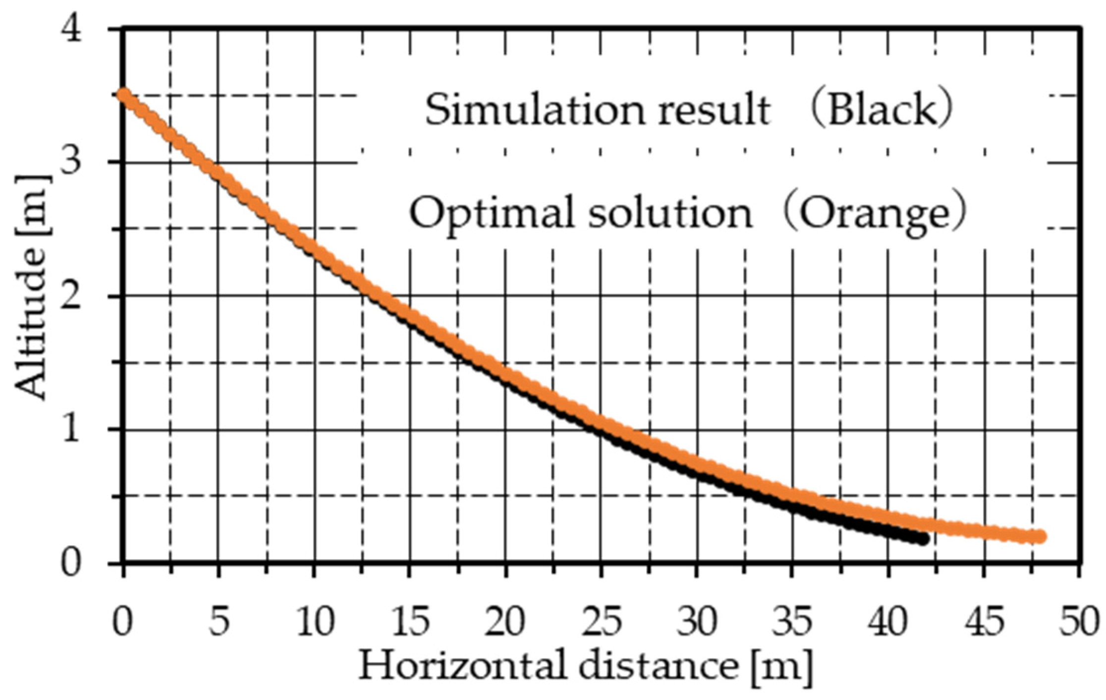
Figure 5, Figure 6, Figure 7, Figure 8, Figure 9, Figure 10 and Figure 11 below show the optimal solutions for the state and control variables. Figure 5 shows the relationship between altitude and horizontal distance, which indicates that the UAV starts to fly at an initial altitude of 3.51 m and then arrives at a terminal altitude of 0.2 m, and the total horizontal distance from the start to the terminal is confirmed as 47.9 m. As shown in Figure 5, Figure 6, Figure 7, Figure 8, Figure 9 and Figure 10, the terminal time was 1.95 s. Figure 6 shows the time histories of the pitch angle, path angle, and angle of attack. The pitch angle rose from the initial value of −9.07 degrees to −1.74 degrees, and the initial value of the path angle was −7.0 degrees since the glide slope angle was set to 7.0 degrees. The calculated terminal value of the path angle is confirmed as −0.41 deg. As shown in Figure 7, there was a slight deceleration in the horizontal direction, and the terminal value was confirmed as 24.0 m/s. 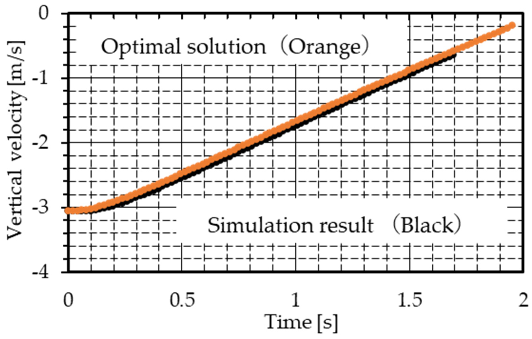As shown in Figure 8, there was a deceleration in the vertical direction, and the terminal value is confirmed as −0.17 m/s. 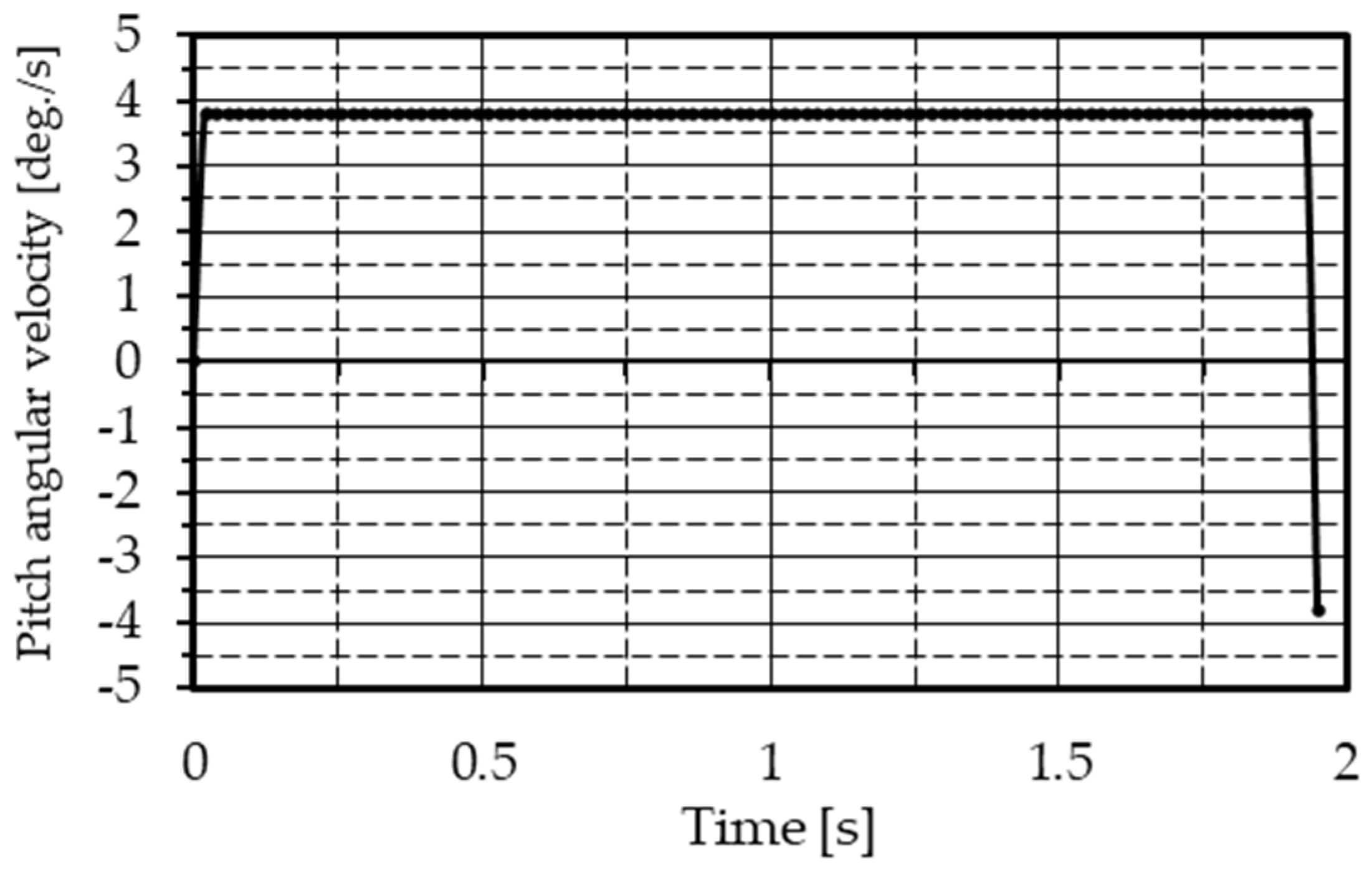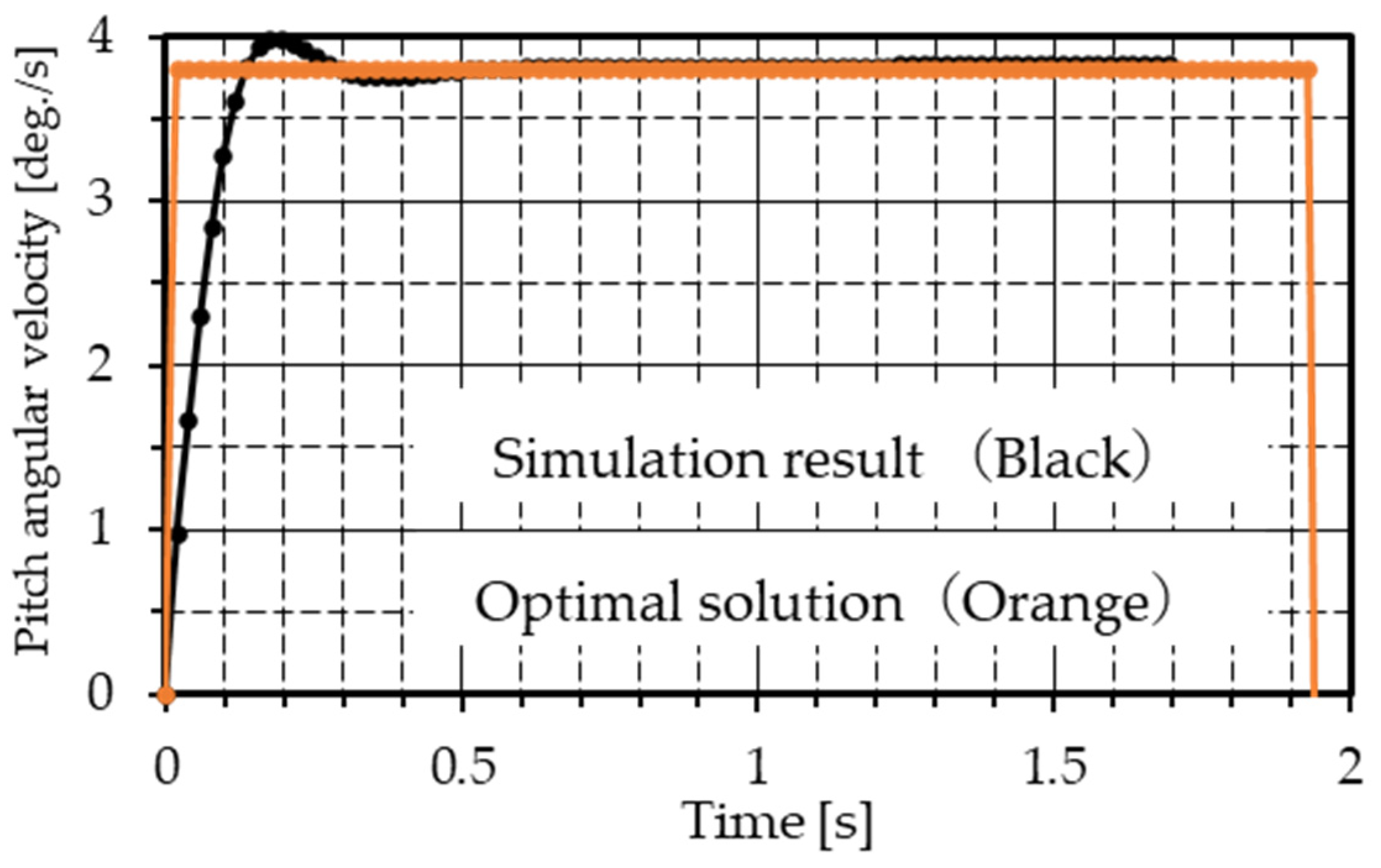As shown in Figure 9, the initial value of the pitch angular velocity is confirmed as 0.0 deg./s, the terminal value is confirmed as −3.8 deg./s, and the points other than the endpoints are confirmed as 3.8 deg./s. So, the pitch angular velocity is generated in the direction of nose-up. 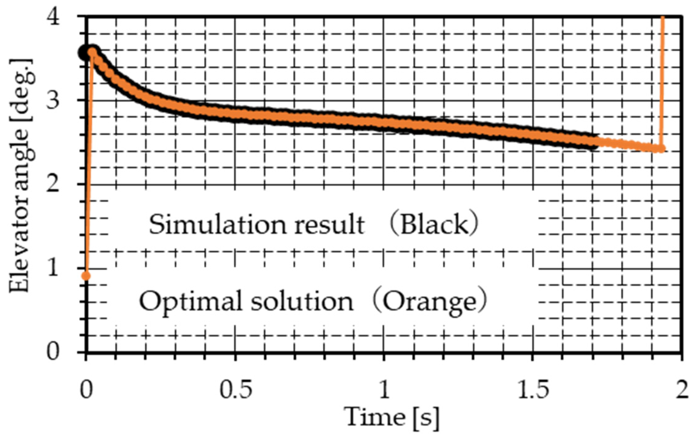As shown in Figure 10, there is divergence between the numerical solutions of the initial and terminal values of the elevator angle. The points other than the endpoints are positive values, and these gradually decrease. In Figure 11, the flare time constant is confirmed as 1.15 s and is constant. The obtained flare time constant is the value at which a path close to the ideal exponential type of path of the flare is realized while minimizing the horizontal distance during the flare phase.

Therefore, the optimized flare time constant ${\tau }_{\mathrm{o}\mathrm{p}\mathrm{t}}$ is set as 1.15 s.

Although this study evaluates the proposed method under a single flight condition, this condition represents a typical condition for the target high-speed fixed-wing UAVs. As a result, the findings provide valuable insights into practical applications. Furthermore, even if parameters such as the glide slope angle or initial speed at the start of the flare phase were changed, the overall airplane behavior is expected to remain largely unchanged. This is because the first term of the evaluation function in Equation (13) compels the airplane to follow an ideal exponential trajectory across different flight conditions. Therefore, the characteristics of the optimal solutions, including altitude, speeds, and attitude angles, are anticipated to remain consistent under varying conditions.

3.4. Confirmation Through Longitudinal Flight Simulation

In this section, both the accuracy of the optimal solution obtained in Section 3.3 and the validity of the motion model used in the nonlinear optimization problem are evaluated. For this, the optimal solution obtained in Section 3.3 is compared with the simulation results obtained by adding the time-series data for the elevator angle. The results obtained for the longitudinal flight simulation are assumed to be the true values, and the accuracy of the optimal solution can be confirmed through comparison with these values. The validity of the motion model is finally assessed based on this assessment of accuracy. The procedure for longitudinal flight simulation was developed by us using MATLAB [23] and Simulink [24] and does not include lateral motion or landing control systems.

3.4.1. Conditions for Longitudinal Flight Simulation

The time-series data for the elevator angle in Figure 10 are used as the input in the longitudinal flight simulation. However, the numerical solution for the endpoints of the elevator angle diverged, so the value of the endpoints was set to the same value as the value of the next node. The sample time for the longitudinal flight simulation was set to 0.01969 s, the same as the time interval between the nodes for the optimal solution, and the initial altitude was set at the same value as the initial value for the optimal solution. The thrust is set as 6.35 N, the same as in the conditions set for the nonlinear optimization problem. The condition for stopping the longitudinal flight simulation is an altitude of 0.2 m.

3.4.2. Results for Longitudinal Flight Simulation

The simulation results are shown in Figure 11, Figure 12, Figure 13, Figure 14, Figure 15 and Figure 16. Each figure shows the optimal solution (orange) in Section 3 and the time history (black) of the so-called true value when the elevator angle shown in Figure 10 of Section 3 is used as the input in the longitudinal flight simulation. Figure 12 shows the elevator angle, and the elevator angle input in the simulation corresponds to the optimal solution value up to 1.69 s. The results of this simulation imply that an altitude of 0.2 m is reached at 1.69 s when inputting the elevator angle of the optimal solution, and the terminal time of the optimal solution is confirmed as 0.26 s larger than the true value. Figure 13 shows the relationship between altitude and horizontal distance, and the horizontal distance of the optimal solution is confirmed to be about 6.1 m larger than the true value. Figure 14 shows the time history of the vertical velocity based on the simulation and the vertical velocity of the optimal solution. The difference between the two ranges from about 0.002 m/s to 0.07 m/s, with the latter value smaller than the former and with a longer descent time. Because of this difference, the time until touchdown according to the optimal solution becomes longer than that determined from the simulation. Figure 15 shows the pitch angle, which for the optimal solution, ranges from about 0.04 degrees to about 0.17 degrees, which is lower than the true value. Figure 16 shows the pitch angular velocity. The difference between the optimal solution and the true value is large until about 0.5 s from the zero-second point, and the maximum deviation is about 2.8 degrees/s. Since the pitch angle is the value obtained by integrating the pitch angular velocity, the result in Figure 15 shows that the pitch angle up to the point of touchdown obtained using the optimal solution is larger than that obtained from the simulation.

From the above results, the accuracy of the optimal solution is found to decrease at the initial node, at the terminal node, and around those nodes but remains sufficient at other nodes. The reason for this is that, for the Hermite–Simpson collocation method, which is a discretization method, dynamic constraints are not imposed on the endpoints, and the equations of motion of the system are not satisfied at those points. However, the error in the horizontal distance is about 6.1 m, which is less than 1% of the total landing distance and considered negligible. In addition, the transient response of the landing control system is added in the process of the optimal solution. Therefore, it is concluded that the motion model used in the nonlinear optimization problem, described in Section 2 of this paper, is appropriate.

4. Verification Using Simulation of a 6-DOF Flight

In this section, a simulation is used to confirm both the validity of the method for determining the flare time constant by solving an optimal control problem using a motion model approximated to three degrees of freedom and the feasibility of safe touchdown by controlling the airplane according to the descent rate command determined by the optimal flare time constant ${\tau }_{\mathrm{o}\mathrm{p}\mathrm{t}}$ under conditions close to the real environment. Also, the effectiveness of the proposed method in design is demonstrated by comparing the landing distances with a general flare time constant and an optimally set flare time constant. The simulation involves paths from the glide slope phase to the flare phase carried out according to a six-degrees-of-freedom flight motion, and it was internally developed by us using MATLAB [23] and Simulink [24] and incorporates the coupling between the angular velocities (p, q, r) in rotational motion, as well as the coupling between the translational velocities (u, v, w) and the angular velocities (p, q, r) in translational motion. Additionally, the aerodynamic forces and moments include the quadratic dependence on velocity, meaning that second-order terms are not neglected.

4.1. Conditions for 6-DOF Flight Simulation

The initial flight conditions for the glide slope phase of the UAV are the same as those for the level-flight phase. Hence, the longitudinal equilibrium equation is solved by setting the left side of Equations (1)–(3) to zero and substituting a path angle of zero degrees so as to calculate the pitch angle, angle of attack, and elevator angle during level flight. In solving the longitudinal equilibrium equation, it is assumed that the UAV is flying at an airspeed of 25 m/s, a roll angle of zero degrees, and a heading angle of zero degrees with a steady wind for which the parameters are summarized in

Table 8. Variables included in the steady wind model equation.

Variable	Value
$h_{\mathrm{o}}$	6.0 m
$n$	7.0
$V_{\mathrm{o}\_\mathrm{w}\mathrm{i}\mathrm{n}\mathrm{d}}$	2.7 m/s

. In addition, the initial position was also set as 0 m of the initial X position, 1.0 m of the initial Y position, and 90.0 m of the initial Z position. The glide slope angle is set as 7.0 degrees, which is the set value when determining the initial conditions for the optimal control problem in Section 3.2. The altitude $h_{\mathrm{t}\mathrm{r}}$ when transitioning from the glide slope phase to the flare phase is calculated from Equation (17). The terminal condition of the flare phase, i.e., the touchdown altitude $h_{\mathrm{t}\mathrm{o}\mathrm{u}\mathrm{c}\mathrm{h}}$, is set in the same way as Table 5. These values are summarized in

Table 9. Simulation conditions.

Variable	Value
${\theta }_{\mathrm{s}0}$	−2.0 deg.
${\varphi }_{\mathrm{s}0}$	0.0 deg.
${\psi }_{\mathrm{s}0}$	0.0 deg.
${\alpha }_{\mathrm{s}0}$	−2.0 deg.
${\delta e}_{\mathrm{s}0}$	3.86 deg.
$X_0$	0.0 m
$Y_0$	1.0 m
$Z_0$	90.0 m
${\theta }_{\mathrm{G}\mathrm{S}}$	7.0 deg.
${\tau }_{\mathrm{o}\mathrm{p}\mathrm{t}}$	1.15 s
$h_{\mathrm{t}\mathrm{r}}$	3.5 m
$h_{\mathrm{t}\mathrm{o}\mathrm{u}\mathrm{c}\mathrm{h}}$	0.2 m

.

Target UAV systems are subject to uncertain factors such as wind and sensor noise. These were reproduced in the six-degrees-of-freedom flight simulation. Sensor noise was added to the attitude angle data (pitch angle, roll angle, and yaw angle) and airspeed data. For the accuracy of the attitude angle, we referred to the catalog values for INS systems in [25], and regarding the airspeed accuracy, we referred to the values measured by a wind tunnel test facility. These values are summarized in

Table 10. Sensor accuracy reproduced in simulation.

Anticipated Sensor	Accuracy
INS (pitch, roll, yaw)	$\pm 0.5 \mathrm{d}\mathrm{e}\mathrm{g}.\left(1\sigma \right)$
ADS	$\pm 1.5\mathrm{m}/\mathrm{s}\left(1\sigma \right)$

. In simulations, the steady wind model and the continuous gust model [26] are used as wind models, where it is assumed that the steady wind blows parallel to the ground surface. The magnitude of the steady wind $V_{\mathrm{s}\mathrm{t}\mathrm{e}\mathrm{a}\mathrm{d}\mathrm{y}}$ is determined by the power law of wind velocity shown in Equation (23) and is dependent upon altitude [27]. The direction of the steady wind is set at a 30-degree azimuth. The values used in Equation (23) are summarized in Table 10. In the continuous gust model, the Dryden turbulence model is used to express the magnitude of turbulence on each axis.

$$V_{\mathrm{s}\mathrm{t}\mathrm{e}\mathrm{a}\mathrm{d}\mathrm{y}}={\left({\displaystyle \frac{h}{h_{\mathrm{o}}}}\right)}^{{\displaystyle \frac{1}{n}}}{V}_{\mathrm{o}\_\mathrm{w}\mathrm{i}\mathrm{n}\mathrm{d}}$$

(23)

Only newly introduced variables included in Equation (23) are defined here.

$h_{\mathrm{O}}$ represents the ground height of the observation point in meters. $n$ represents the parameter of the power law. $V_{\mathrm{O}\_\mathrm{w}\mathrm{i}\mathrm{n}\mathrm{d}}$ represents the windspeed at the observation point in meters per second.

4.2. Flight Control System of a UAV During Landing

The 6-DOF flight simulation is carried out for verification of the landing phase, which consists of the glide slope phase and the flare phase. A glide slope control system is used in the glide slope phase, and a flare control system is used in the flare phase. Each control system is composed of a longitudinal motion control system and a lateral motion control system. The block diagram of the longitudinal motion control system of the glide slope control system is shown in Figure 17, and the block diagram of the longitudinal motion control system of the flare control system is shown in Figure 18. The lateral motion control system, which is commonly used in glide slope and flare control systems, is shown in Figure 19. In addition, PID control laws are used in all control systems.

The longitudinal motion control system in the glide slope phase adjusts the pitch angle using the elevator to match the value designated by commands in accordance with the deviation from the target flight trajectory. In addition, it adjusts the thrust to the value designated by the commands, in accordance with the deviation from the target airspeed.

In the control system for longitudinal motion during the flare phase, the descent rate is used as a command. The descent rate command is generated using the current altitude and the optimized flare time constant. Commands for the pitch angle are generated according to the deviation from the descent rate. Similarly, as for the glide slope control system, the commands for thrust are generated according to the deviation from the target airspeed.

The lateral motion control system adjusts the roll angle to the value designated by commands using the aileron, in accordance with the deviation from the center line of the runway.

4.3. Results of the 6-DOF Flight Simulation

The simulation results from the start of the glide slope phase to touchdown are shown in Figure 19, Figure 20, Figure 21, Figure 22, Figure 23, Figure 24, Figure 25, Figure 26 and Figure 27.

4.3.1. Entire Landing Trajectory

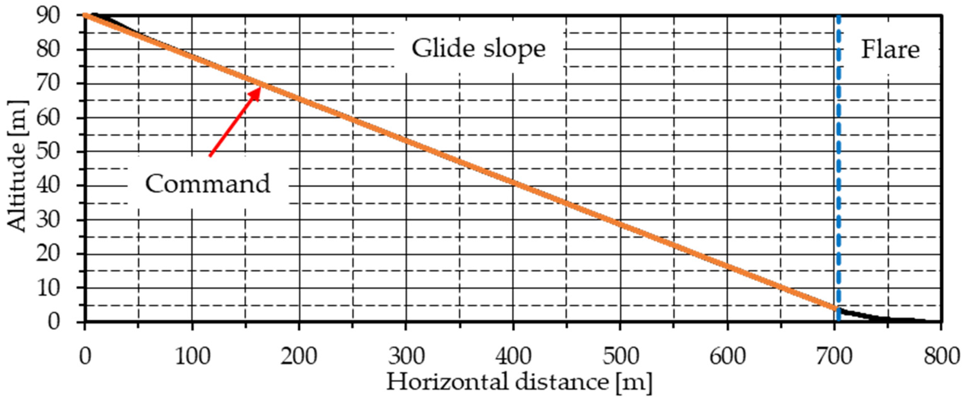
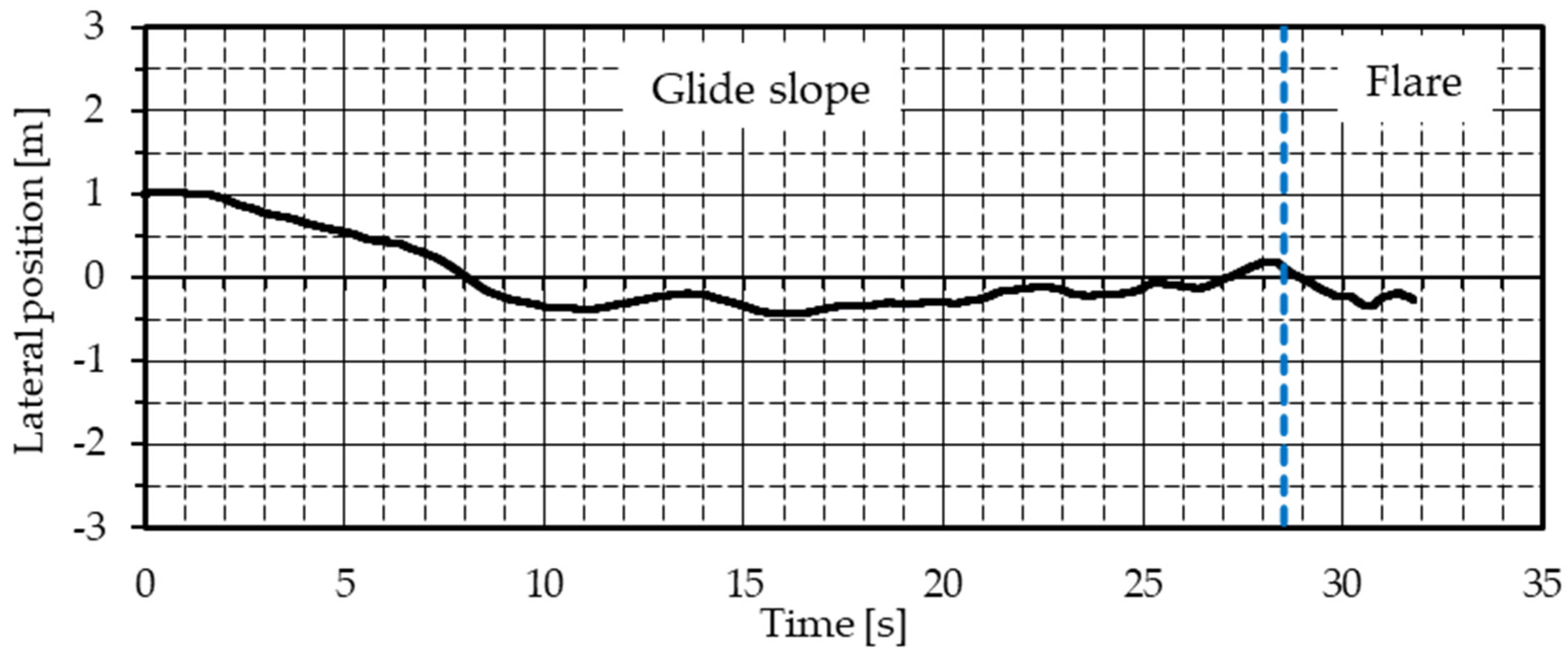
Figure 20 shows the entire landing trajectory from the start of the glide slope phase to the flare phase. During the glide slope phase, the UAV slightly exceeded the command value up to the first horizontal distance of 50 m but then adhered to the command value. Figure 21 shows the lateral position. Although there is an initial deviation of 1.0 m and wind disturbance is included, the UAV is flying along the center of the runway, and the lateral motion control system is functioning well.

4.3.2. Glide Slope Phase

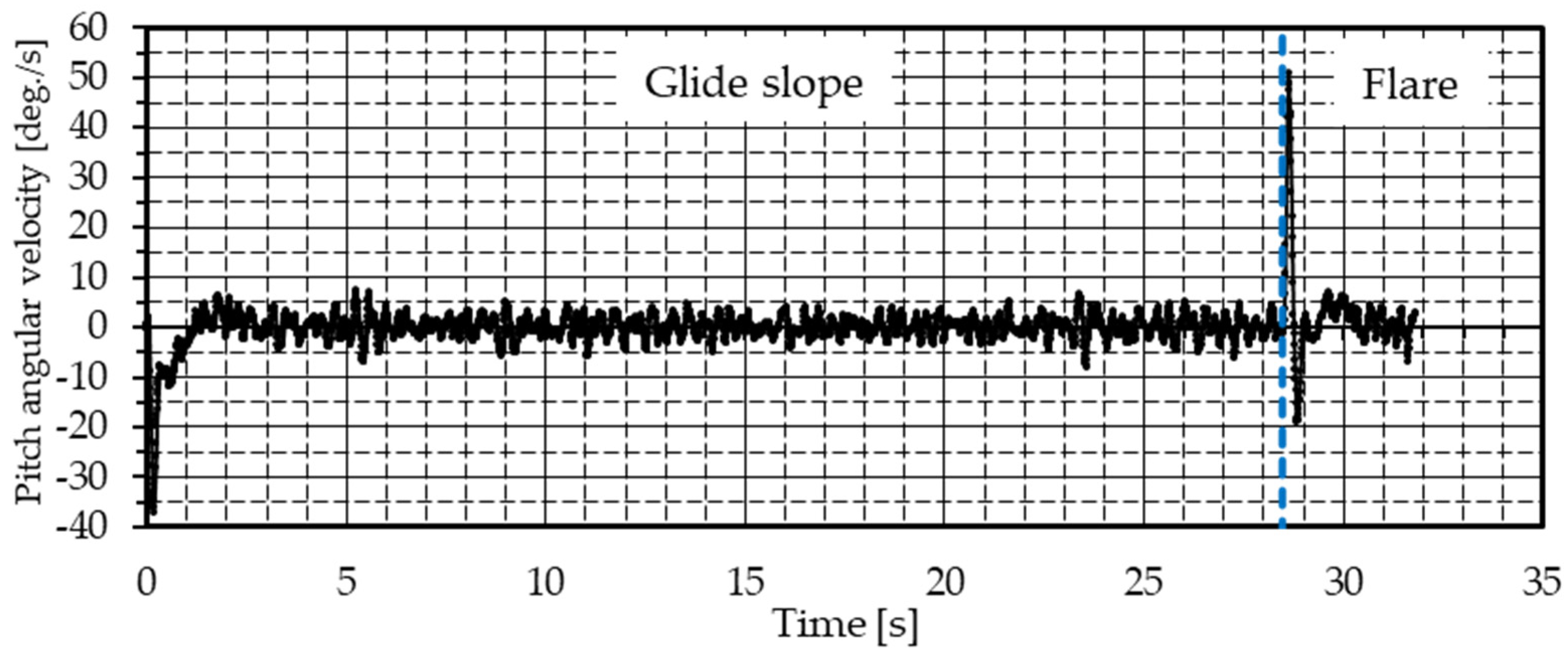
Figure 22 shows the pitch angle, and during the glide slope phase, there is a delay in response to commands until about 3 s after the start, after which it instantaneously responds to the commands. The average pitch angle between 20 and 25 s is confirmed as −10.08 deg., which is fairly consistent with the initial conditions for the pitch angle set in the nonlinear optimization problem. Figure 23 shows the pitch angular velocity, and it is balanced at around zero deg./s in the latter half of the glide slope phase. Figure 24 shows the elevator angle, and the average elevator angle between 20 and 25 s of the glide slope phase is confirmed as 3.95 deg, which is approximately the same as the elevator angle during balance shown in Table 4. Figure 25 shows the airspeed, which remained at about a 25 m/s constant during the glide slope phase. Figure 26 shows the thrust, which was constant at about 6.0 N during the glide slope phase from about 16 s to 28 s. This thrust value is approximately the same as the thrust value during balance shown in Table 4.

4.3.3. Flare Phase

Figure 22 shows the pitch angle, and the UAV follows the command. And the nose is raised up to a pitch angle of −1.63 deg. Figure 23 shows the pitch angular velocity, and when the transition from the glide slope phase to the flare phase occurs, the pitch angular velocity reaches a maximum of 50.7 deg./s. Figure 25 shows the airspeed, and the airspeed decreases slightly during the flare phase. This trend in the flare phase is consistent with the calculation results for the horizontal and vertical velocities in the nonlinear optimization problem in Section 3 (Figure 6 and Figure 7). Figure 26 shows the thrust, which increased to a maximum of 13.7 N during the flare phase. The increase in thrust during the flare phase is consistent with the decrease in airspeed, as shown in Figure 25.

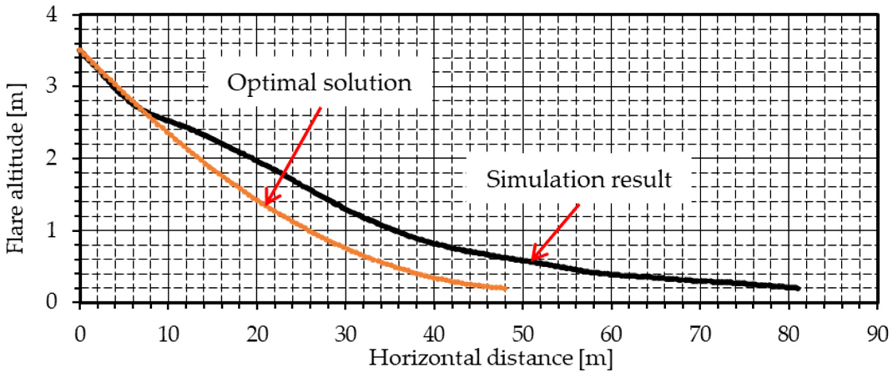
Figure 27 shows only the flare path in Figure 20 and the optimal solution for the flare path described in Section 3, and a comparison of the optimal flare path with the flare path in the 6-DOF flight simulation. After the flare starts, the UAV follows almost the same path until it reaches a horizontal distance of about 6 m, after which the simulation results show that the rate of descent decreases, and the terminal horizontal distance is 33.0 m greater than that for the optimal solution. 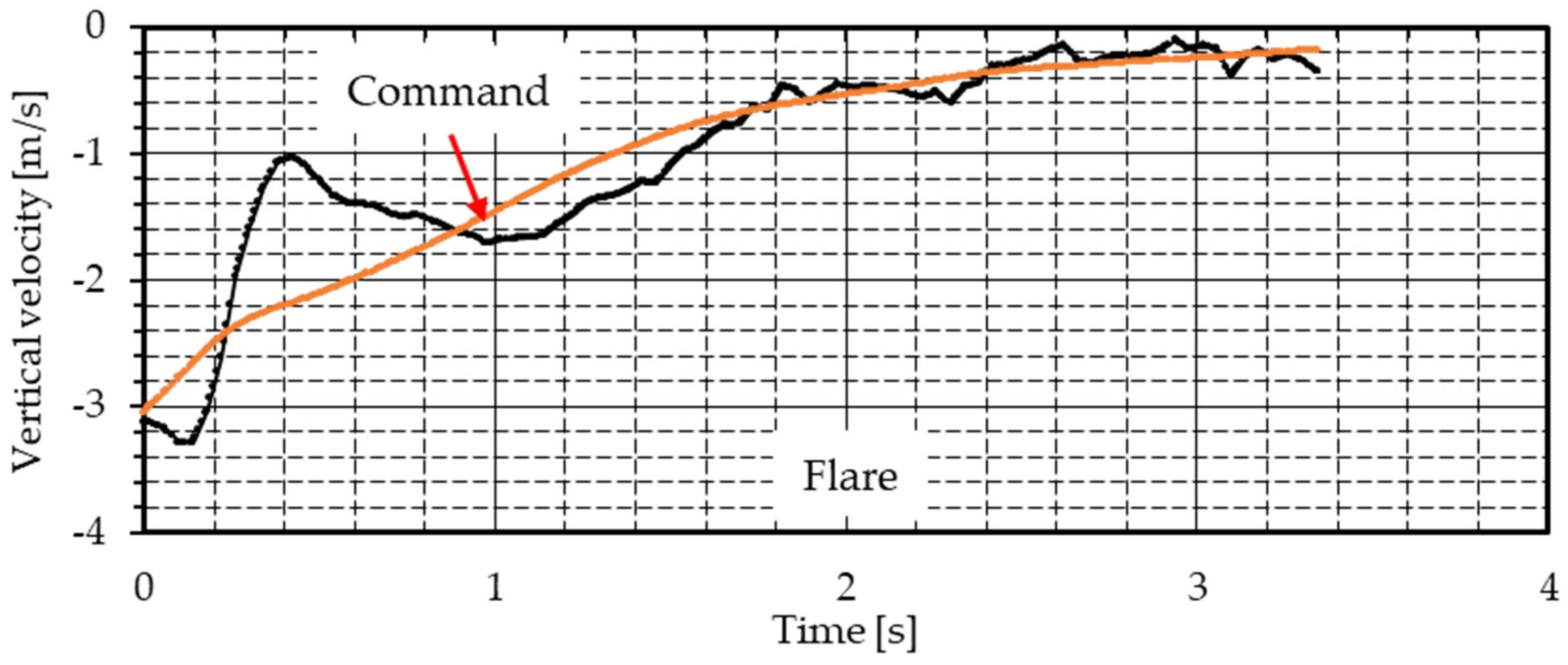Figure 28 shows the vertical velocity (descent rate). The flare phase is controlled by the descent rate command calculated using Equation (24), which includes the variables for current altitude and the flare time constant ${\tau }_{\mathrm{o}\mathrm{p}\mathrm{t}}$ determined in Section 3. Although the time history of the descent rate is a transient response until about 1.8 s, it subsequently converges to the command value. At touchdown, the vertical velocity (descent rate) was −0.34 m/s, achieving the target descent rate suppression of −1.0 m/s or more and 0.0 m/s or less.

From these results, it is concluded that the method for determining the flare time constant by solving an optimal control problem using a motion model approximated to three degrees of freedom is reasonable, and landing control can feasibly be achieved using the optimized flare time constant.

$${\dot{h}}_{\mathrm{c}\mathrm{m}\mathrm{d}}(t)=-{\displaystyle \frac{h\left(t\right)}{{\tau }_{\mathrm{o}\mathrm{p}\mathrm{t}}}}$$

(24)

4.4. Effectiveness of Applying the Optimized Flare Time Constant

This section compares the landing distances for a typical flare time constant and an optimized flare time constant and quantitatively demonstrates the effectiveness of the proposed method. The typical flare time constant is set at 2 to 5 s [5], and in this study, it is set to 3.5 s. By changing the flare time constant, the switching altitude $h_{\mathrm{t}\mathrm{r}}$ from the glide slope phase to the flare phase is determined as 7.62 m according to Equation (17). However, all other simulation conditions remain as summarized in Section 4.1.

When the flare time constant is set to 3.5 s, the landing distance is 983.9 m, as shown in Figure 29. In contrast, with the optimized flare time constant of 1.15 s, the landing distance is reduced to 785.4 m, as shown in Figure 20, resulting in a 20.2% reduction. Therefore, using the optimized flare time constant calculated by the proposed method is effective in reducing the landing distance.

5. Conclusions

A method for determining the flare time constant, which dominates the curvature of the flare path, is proposed for shortening the landing distance in the flare phase. Using this method, the feasible flare time constant is determined by solving a nonlinear optimization problem using a UAV’s equations of motion as dynamic constraints. We used the derived flare time constant together with the optimized elevator angle in a longitudinal flight simulation to confirm both the accuracy of the optimal solution and the validity of the motion model used in the nonlinear optimization problem. Finally, it was confirmed that the landing control can be feasibly achieved using the optimized flare time constant obtained from the 6-DOF flight simulation. Also, it is confirmed that the proposed method is effective in reducing the landing distance.

References

1. Zhou, Y.; Zhao, H.; Liu, Y. An evaluative review of the VTOL technologies for unmanned and manned aerial vehicles. Comput. Commun. 2020, 149, 356–369. [Google Scholar] [CrossRef]
2. Al-Haj, S.; Husni MA, L.; John, M.; Hamid, M.F.A. Prediction of Take-off and Landing Performance for A Channel-Wing UAV using Lifting-Line Theory. Proc. Aerosp. Soc. Malays. 2023, 1, 13–20. [Google Scholar]
3. Zhang, Y.; Xu, J.; Pan, R.; Li, Y.; Ma, Z.; Huang, S. Numerical investigation of short takeoff and landing exhaust system using bypass dual throat nozzle. Aerosp. Sci. Technol. 2023, 138, 108316. [Google Scholar] [CrossRef]
4. Wu, H.; Wang, Z.; Zhou, Z.; Jia, J.; Wang, R. Modeling of small UAV parachute recovery system based on Lagrangian method. In Proceedings of the 2019 IEEE International Conference on Mechatronics and Automation (ICMA), Tianjin, China, 4–7 August 2019; IEEE: Piscataway, NJ, USA, 2019; pp. 1127–1132. [Google Scholar]
5. Hyokawa, S.; Ueba, M. Design and verification of short-distance landing control system for a one-third-scale unmanned supersonic experimental UAV. Aerospace 2023, 10, 334. [Google Scholar] [CrossRef]
6. Kargın, V. Design of an Autonomous Landing Control Algorithm for a Fixed Wing UAV. Master’s Thesis, Middle East Technical University, Ankara, Türkiye, 2007. [Google Scholar]
7. Boskoski, P.; Mileva, B.; Deskoski, S. Auto landing using fuzzy logic. In Proceedings of the 6th International PhD Workshop on Systems and Control, Izola, Slovenia, 4–8 October 2005. [Google Scholar]
8. Blakelock, J.H. Automatic Control of UAV and Missiles; John Wiley & Sons: Hoboken, NJ, USA, 1991. [Google Scholar]
9. Sadraey, M. Automatic Flight Control Systems; Morgan & Claypool Publishers: San Rafael, CA, USA, 2020. [Google Scholar]
10. Kato, K. Engineering Optimal Control. In Approach to Nonlinearity; Translated from Japanese; The University of Tokyo Press: Tokyo, Japan, 1988. [Google Scholar]
11. Kelly, M. An introduction to trajectory optimization: How to do your own direct collocation. SIAM Rev. 2017, 59, 849–904. [Google Scholar] [CrossRef]
12. Rendón, S.V. Trajectory Planning Based on Collocation Methods for Multiple Aerial and Ground Autonomous Vehicles. Doctoral Dissertation, Universidad de Sevilla, Seville, Spain, 2015. [Google Scholar]
13. Katoch, S.; Chauhan, S.S.; Kumar, V. A review on genetic algorithm: Past, present, and future. Multimed. Tools Appl. 2021, 80, 8091–8126. [Google Scholar] [PubMed]
14. Wang, D.; Tan, D.; Liu, L. Particle swarm optimization algorithm: An overview. Soft Comput. 2018, 22, 387–408. [Google Scholar] [CrossRef]
15. Forsgren, A.; Gill, P.E.; Wright, M.H. Interior methods for nonlinear optimization. SIAM Rev. 2002, 44, 525–597. [Google Scholar] [CrossRef]
16. Boggs, P.T.; Tolle, J.W. Sequential quadratic programming. Acta Numer. 1995, 4, 1–51. [Google Scholar] [CrossRef]
17. Meng, S.; Xiang, J.; Luo, Z.; Ren, Y.; Zhuang, N. A novel trajectory planning strategy for aircraft emergency landing using Gauss pseudospectral method. Control Theory Technol. 2014, 12, 393–401. [Google Scholar]
18. Lee, S.G.; Yang, H.H.; Addo-Akoto, R.; Han, J.H. Transition flight trajectory optimization for a flapping-wing micro air vehicle with unsteady vortex-lattice method. Aerospace 2022, 9, 660. [Google Scholar] [CrossRef]
19. Li, X.; Qi, G.; Zhang, L. Time-varying formation dynamics modeling and constrained trajectory optimization of multi-quadrotor UAVs. Nonlinear Dyn. 2021, 106, 3265–3284. [Google Scholar] [CrossRef]
20. Oosedo, A.; Abiko, S.; Konno, A.; Uchiyama, M. Optimal transition from hovering to level-flight of a quadrotor tail-sitter UAV. Auton. Robot. 2017, 41, 1143–1159. [Google Scholar] [CrossRef]
21. SciPy. Available online: https://scipy.org/ (accessed on 28 November 2024).
22. Kanichiro KA, T.O.; Akio, O.; Kenji, K. Introduction to UAV Dynamics; Translated from Japanese; The University of Tokyo Press: Tokyo, Japan, 2012. [Google Scholar]
23. MATLAB. Available online: https://jp.mathworks.com/products/matlab.html (accessed on 28 November 2024).
24. Simulink. Available online: https://jp.mathworks.com/products/simulink.html (accessed on 28 November 2024).
25. CSM-MG200. Available online: https://www.tkk-air.co.jp/unmanned_aerial_vehicle/motion_sensor_csm-mg200.html (accessed on 28 November 2024).
26. Military Specification, Flying Qualities of Piloted UAVs, MIL-F8795C, Nov. 1980. Available online: http://everyspec.com/MIL-SPECS/MIL-SPECS-MIL-F/MIL-F-8785C_5295/ (accessed on 28 November 2024).
27. Shou, T.; Masumi, K.; Hirotada, N. On the Accuracy of the Power Low Formula for the Vertical Profile of the Wind Speed. Wind. Energy 2006, 30, 86–91. (In Japanese) [Google Scholar] [CrossRef]
Figure 1. Landing path consisting of glide slope phase and flare phase. In Figure 1: GS represents the glide slope; θ G S represents the glide slope angle in radians; h 0 represents the initial altitude at the flare phase in meters; t represents the time during the flare phase in seconds; τ represents the flare time constant in seconds; V 0 represents the initial airspeed at the flare phase in meters per second.
Aerospace 12 00318 g001
Figure 2. Forces and moments acting on a UAV. In Figure 2, L w represents the lift of the main wings in Newtons; L t represents the lift of the horizontal tail in Newtons; D represents the drag in Newtons; T represents the thrust in Newtons; g represents the gravitational acceleration in meters per second squared; m represents the mass in kilograms; α represents the angle of attack in radians; γ represents the pass angle in radians; c represents the mean aerodynamic chord in meters; h c g represents the center of gravity position from the leading edge of the main wings in a dimensionless form; h a c represents the aerodynamic center position from the leading edge of the main wings in a dimensionless form; l t represents the length between the center of gravity and the aerodynamic center of the horizontal tail in meters; and C m 0 represents the pitching moment coefficient around the leading edge in a dimensionless form.
Aerospace 12 00318 g002
Figure 3. Model of the target UAV.
Aerospace 12 00318 g003
Figure 4. Step response of the pitch angle control system.
Aerospace 12 00318 g004
Figure 5. Calculation results for altitude and horizontal distance.
Aerospace 12 00318 g005
Figure 6. Calculation results for pitch angle, path angle, and angle of attack.
Aerospace 12 00318 g006
Figure 7. Calculation results for horizontal velocity.
Aerospace 12 00318 g007
Figure 8. Calculation results for vertical velocity.
Aerospace 12 00318 g008
Figure 9. Calculation results for pitch angular velocity.
Aerospace 12 00318 g009
Figure 10. Calculation results for elevator angle.
Aerospace 12 00318 g010
Figure 11. Calculation results for flare time constants.
Aerospace 12 00318 g011
Figure 12. Simulation results and optimal solution for elevator angle.
Aerospace 12 00318 g012
Figure 13. Simulation results and optimal solution (horizontal distance vs. altitude).
Aerospace 12 00318 g013
Figure 14. Simulation results and optimal solution for vertical velocity.
Aerospace 12 00318 g014
Figure 15. Simulation results and optimal solution for pitch angle.
Aerospace 12 00318 g015
Figure 16. Simulation results and optimal solution for pitch angular velocity.
Aerospace 12 00318 g016
Figure 17. Block diagram of glide slope control.
Aerospace 12 00318 g017
Figure 18. Block diagram of flare control.
Aerospace 12 00318 g018
Figure 19. Block diagram of lateral direction control.
Aerospace 12 00318 g019
Figure 20. Simulation results for altitude and horizontal distance.
Aerospace 12 00318 g020
Figure 21. Simulation results for lateral position.
Aerospace 12 00318 g021
Figure 22. Simulation results for pitch angle.
Aerospace 12 00318 g022
Figure 23. Simulation results for pitch angular velocity.
Aerospace 12 00318 g023
Figure 24. Simulation results for elevator angle.
Aerospace 12 00318 g024
Figure 25. Simulation results for airspeed.
Aerospace 12 00318 g025
Figure 26. Simulation results for thrust.
Aerospace 12 00318 g026
Figure 27. Optimal solution and simulation results for flare path.
Aerospace 12 00318 g027
Figure 28. Simulation results for vertical velocity.
Aerospace 12 00318 g028
Figure 29. Simulation results for altitude and horizontal distance ( τ = 3.5   s ).
Aerospace 12 00318 g029