
Modal Phase Study on Lift Enhancement of a Locally Flexible Membrane Airfoil Using Dynamic Mode Decomposition


Abstract
1. Introduction
2. Methodology
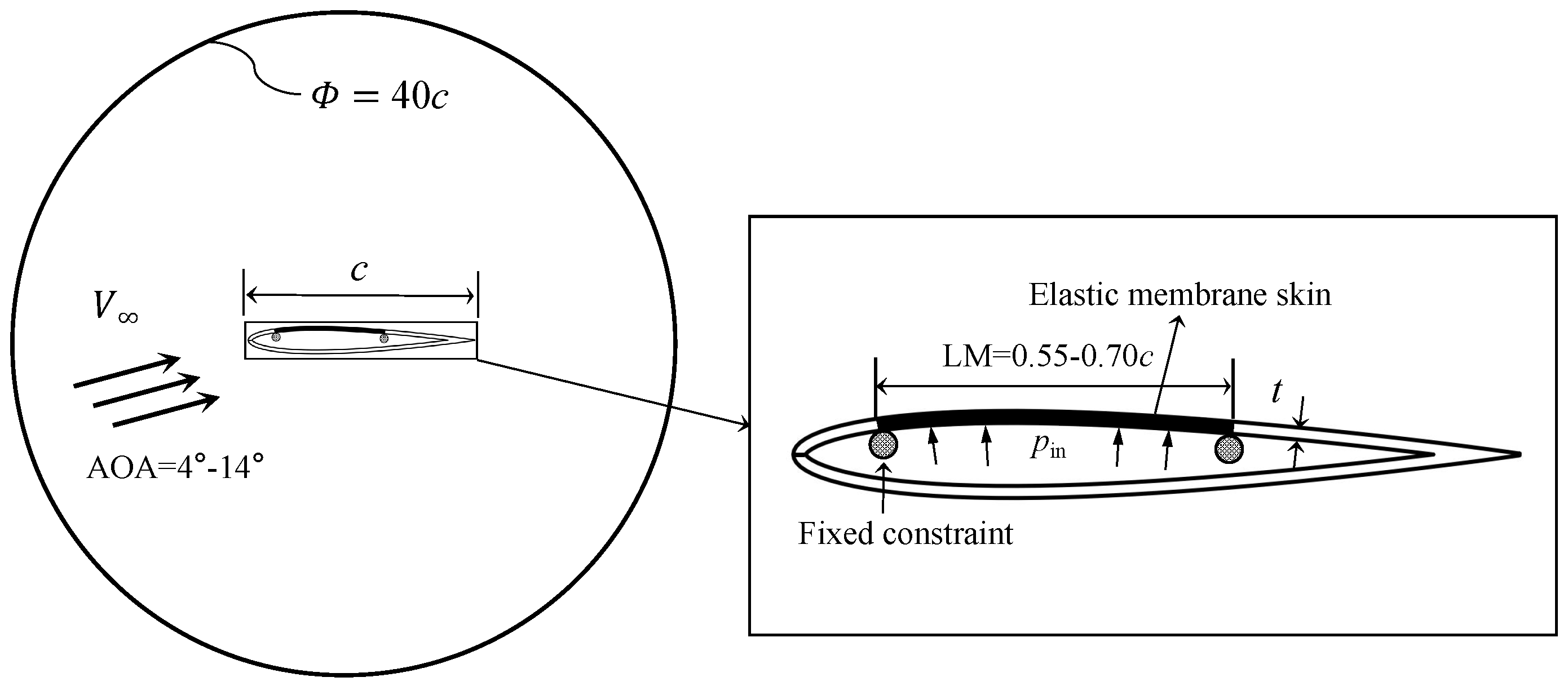
2.1. Computation Model and Setup
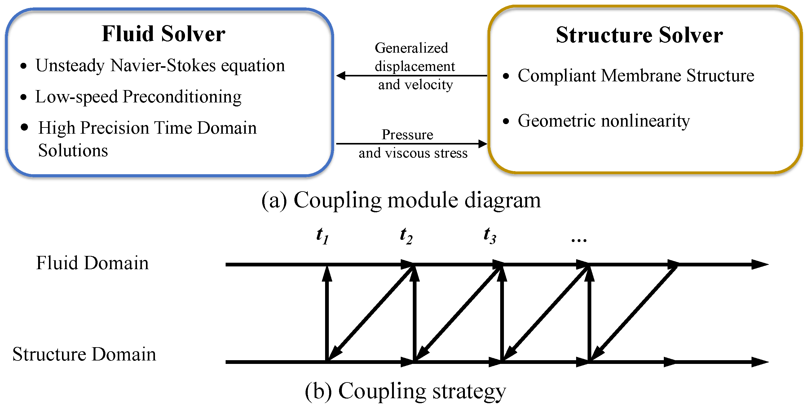
2.2. Aeroelastic Model and Solver
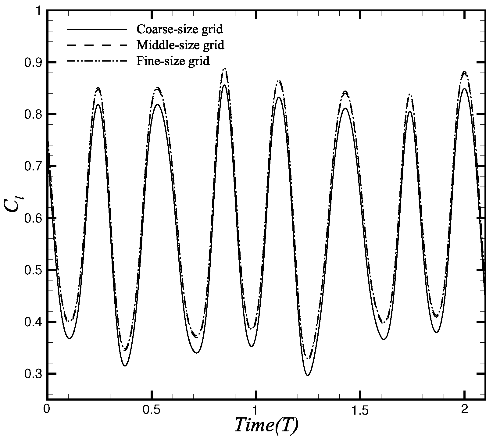
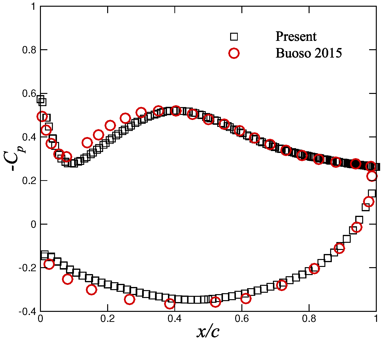
2.3. CFD/CSD Coupling Verification
2.4. Dynamic Mode Decomposition
3. Coupling Response
3.1. Aerodynamic Performance Comparison
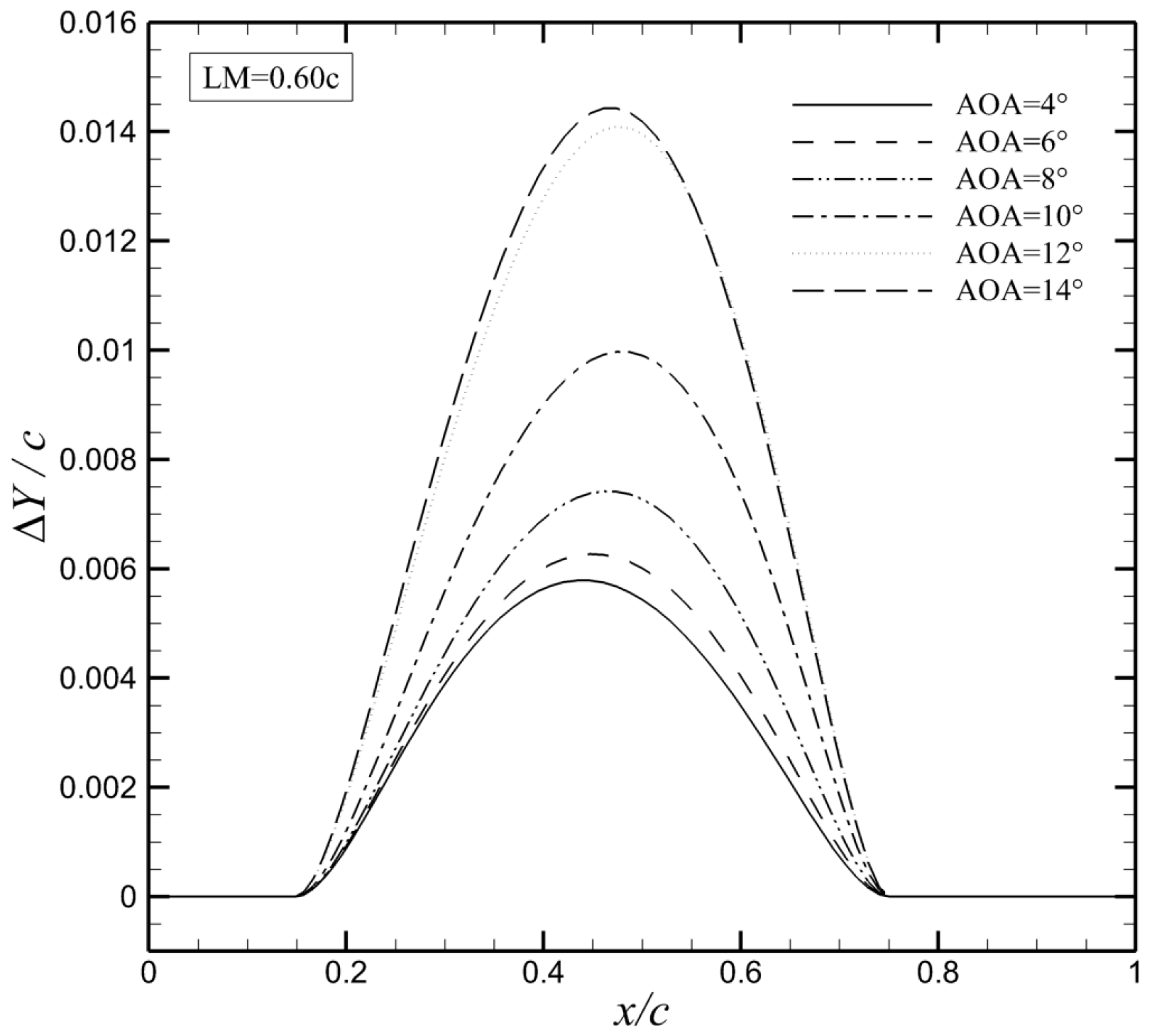
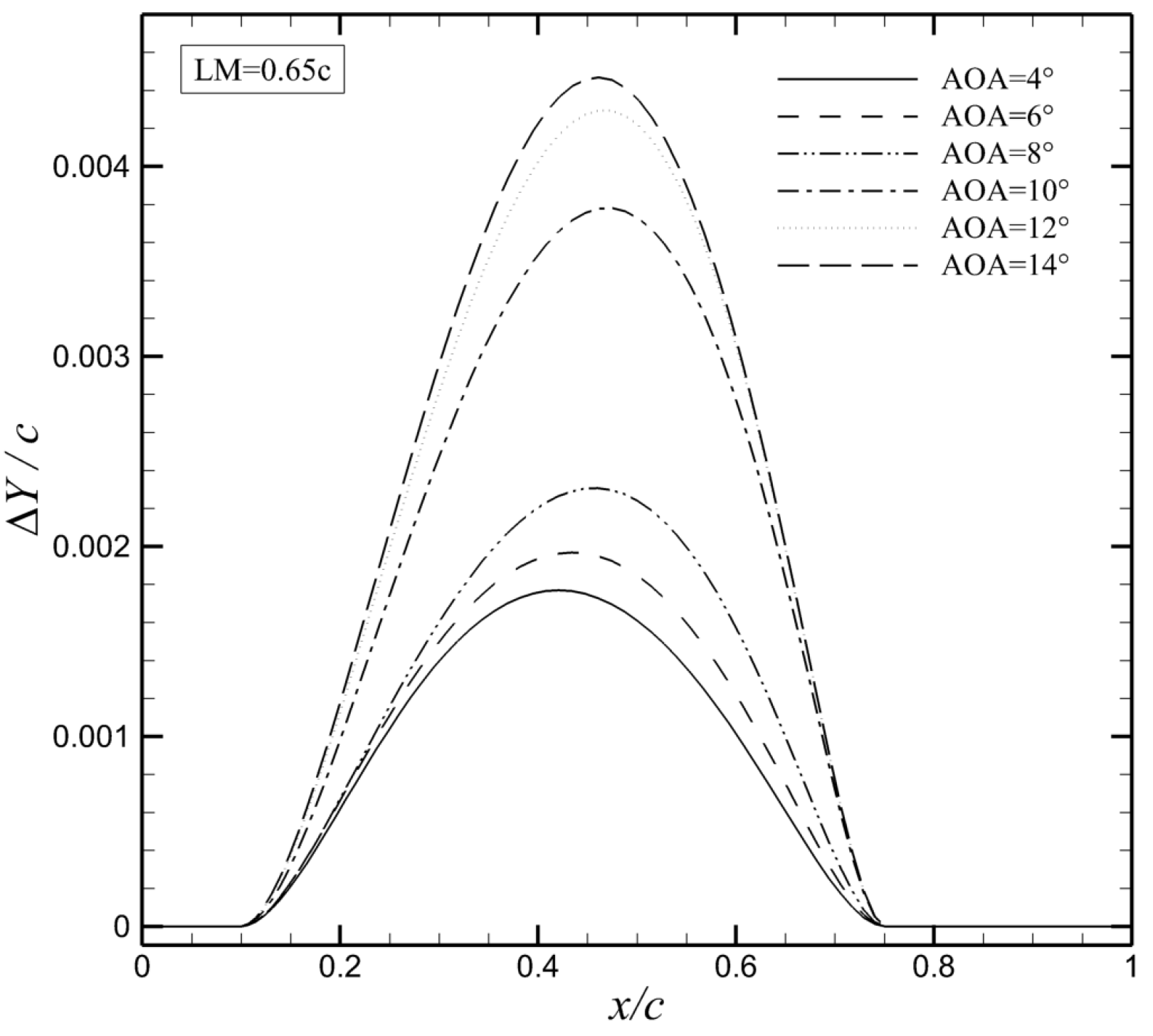
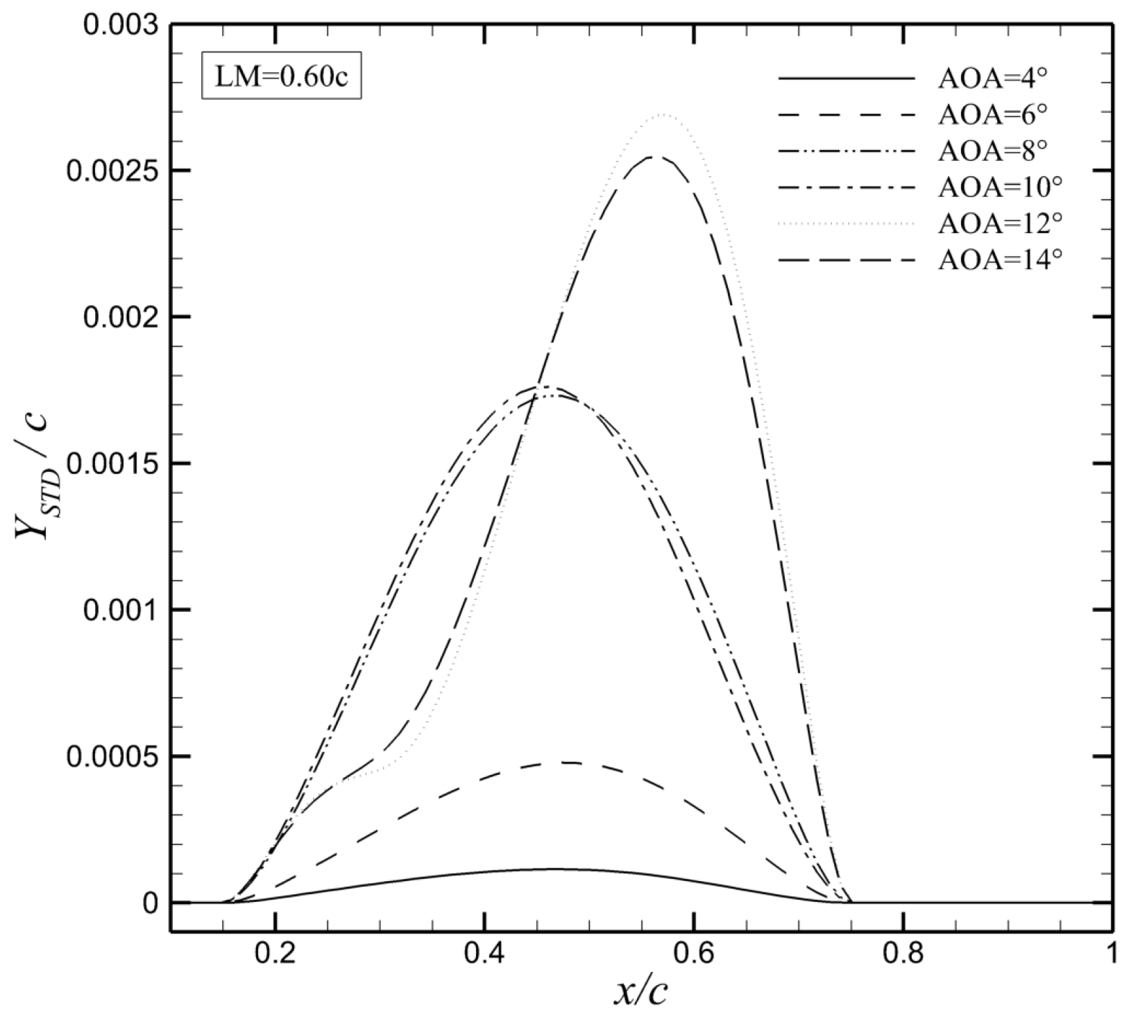
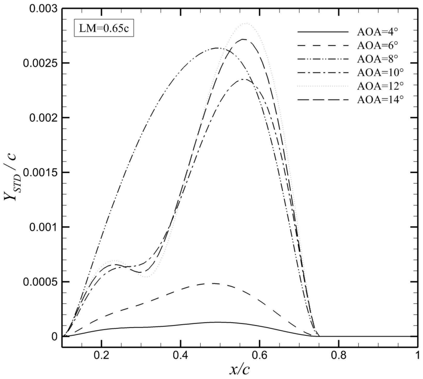
3.2. Structural Responses
4. Dynamic Mode Decomposition Results and Analysis
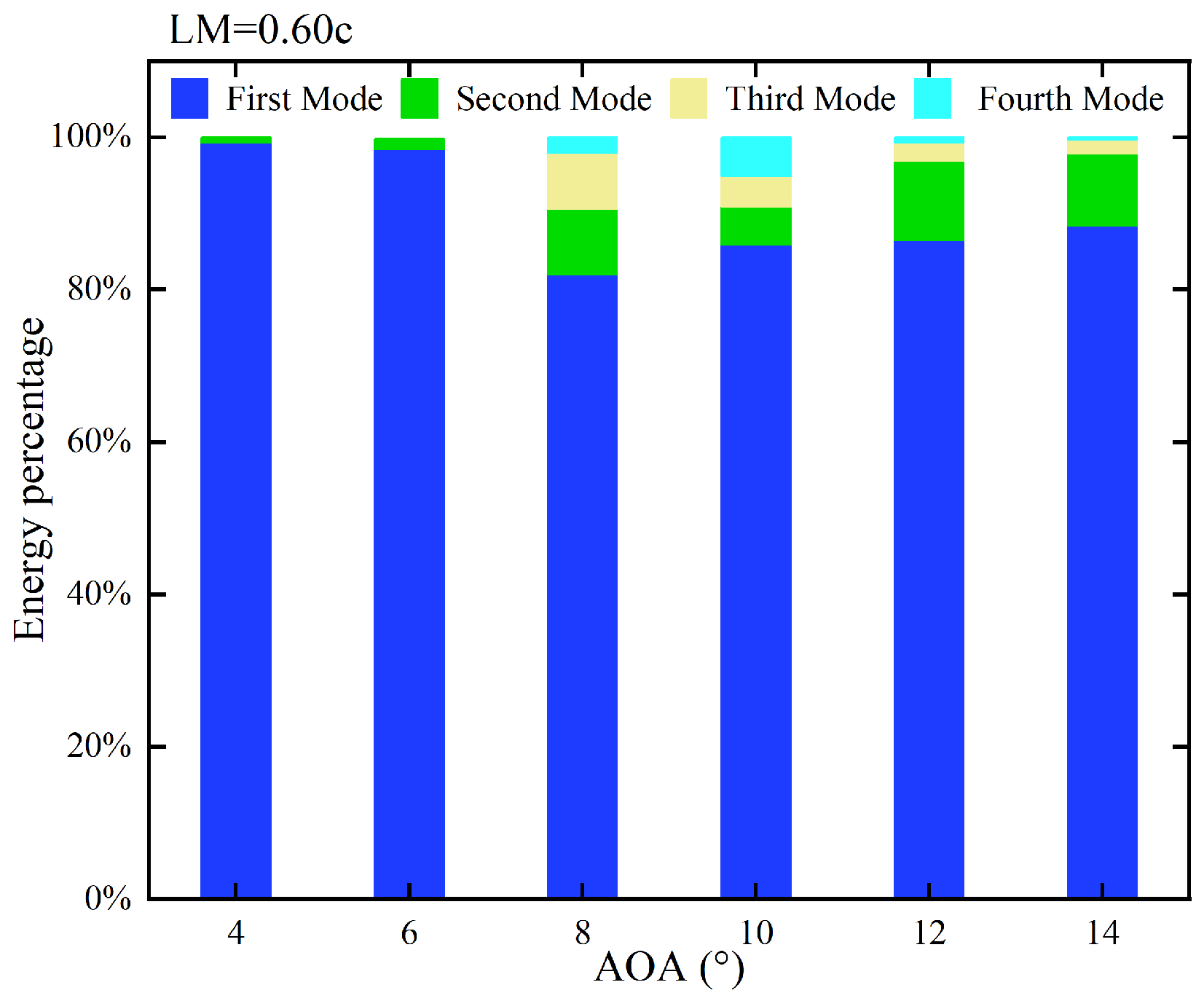
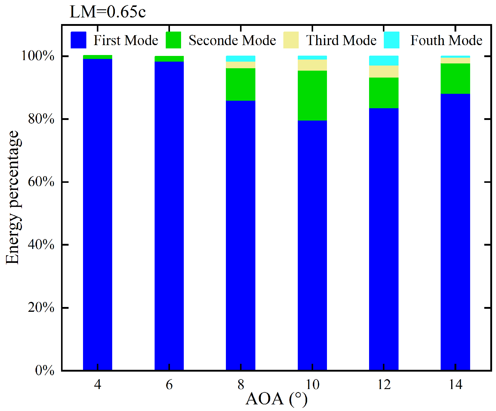
4.1. Modal Shape Results and Analysis
4.2. Modal Phase Results and Analysis
5. DMD Phase-Based Coherent Pattern Analysis
6. Conclusions
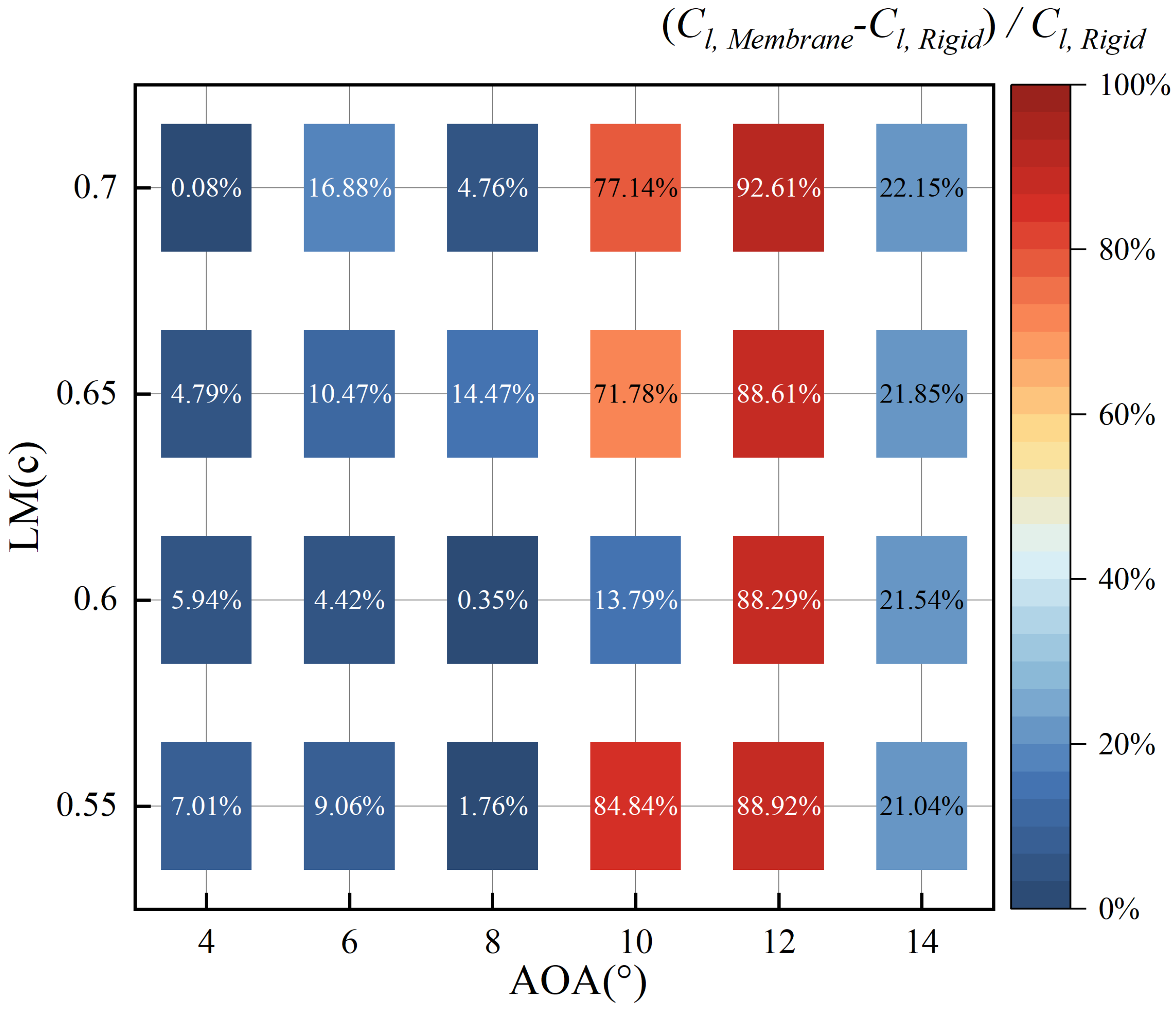
- (1)
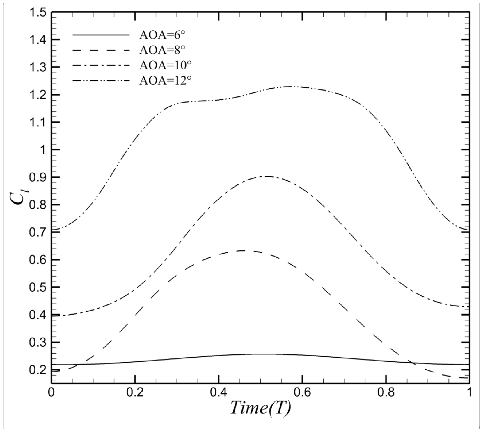
- The elastic membrane airfoil shows different lift enhancement at various AOAs and LMs. The lift coefficients of all membrane airfoils are increased compared to the rigid airfoil. The lift coefficient of the elastic membrane airfoil increases by 92.61% compared to the rigid airfoil at AOA = 12° and LM = 0.70c. Moreover, the lift enhancement exhibits considerable variation as AOA ranges from AOA =68° to 12° and LM ranges from 0.60c to 0.65c.
- (2)
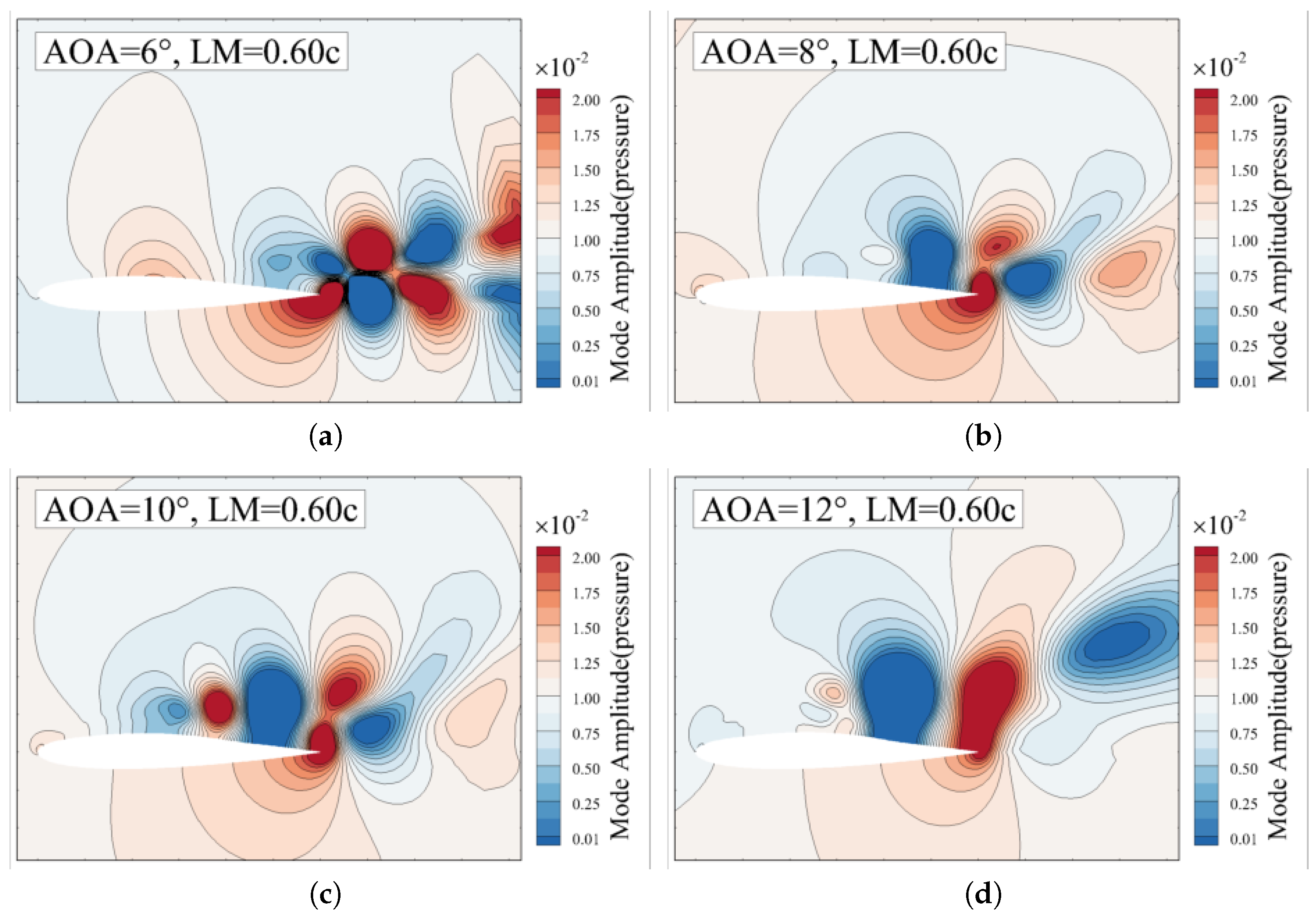
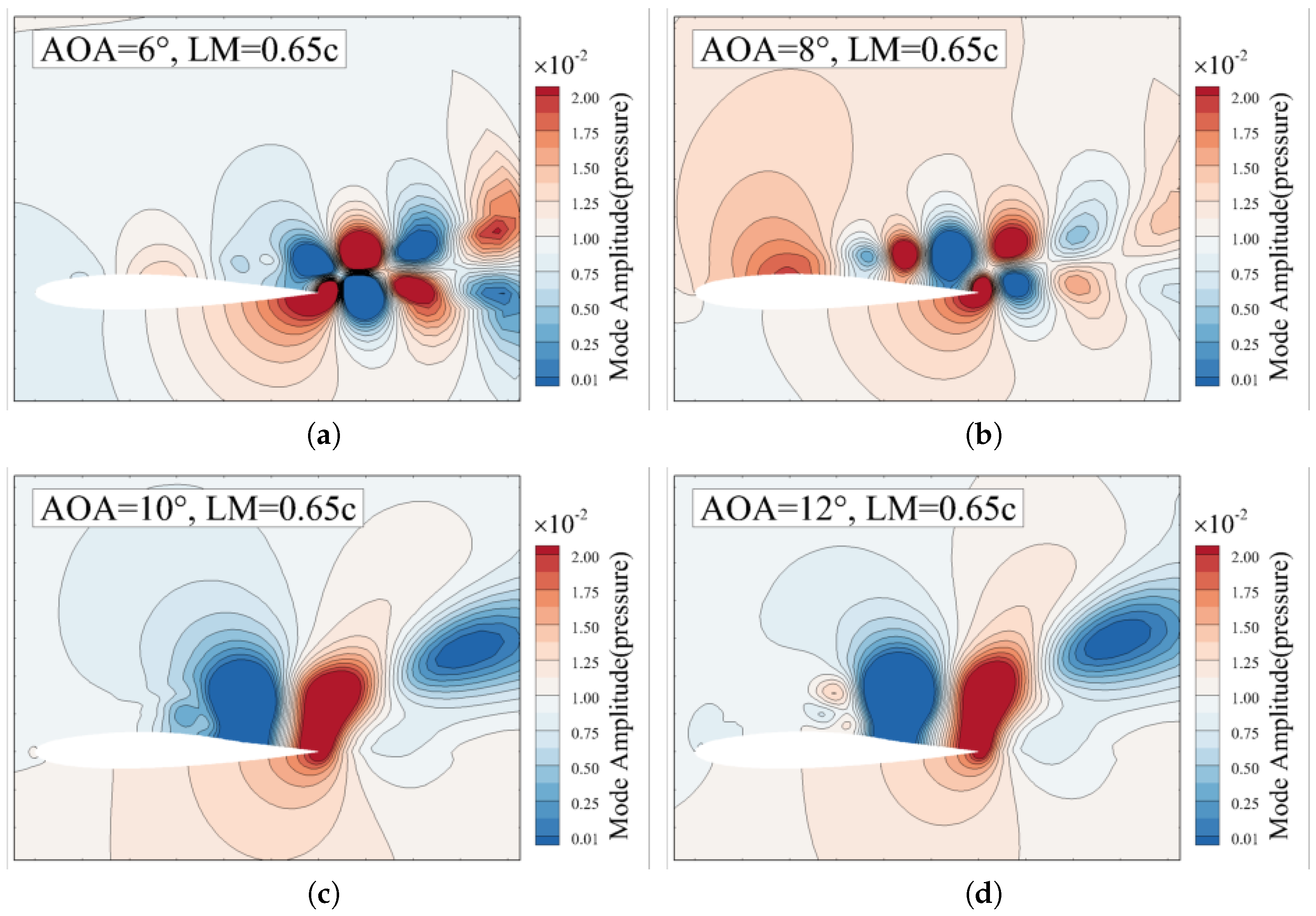
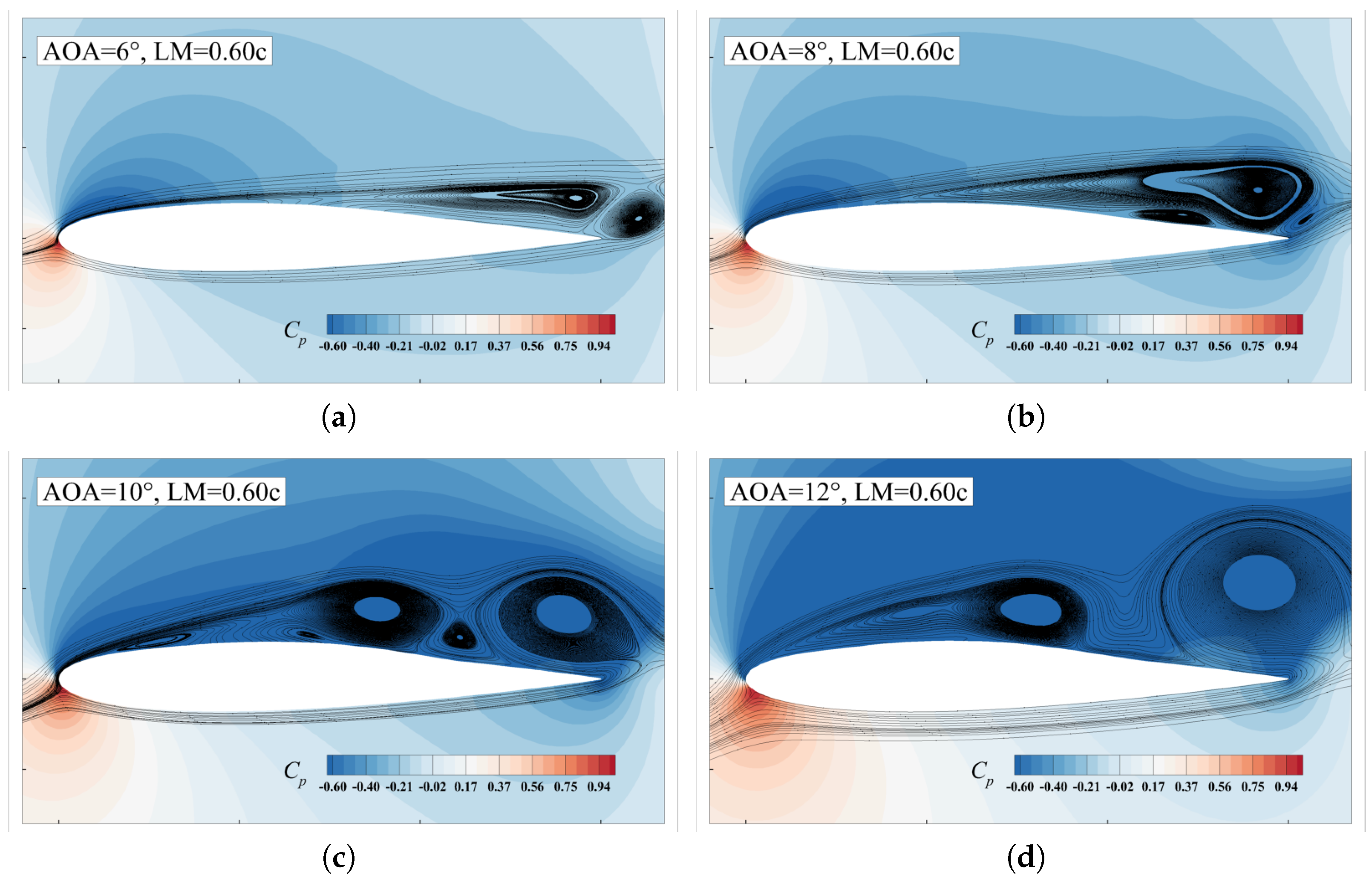
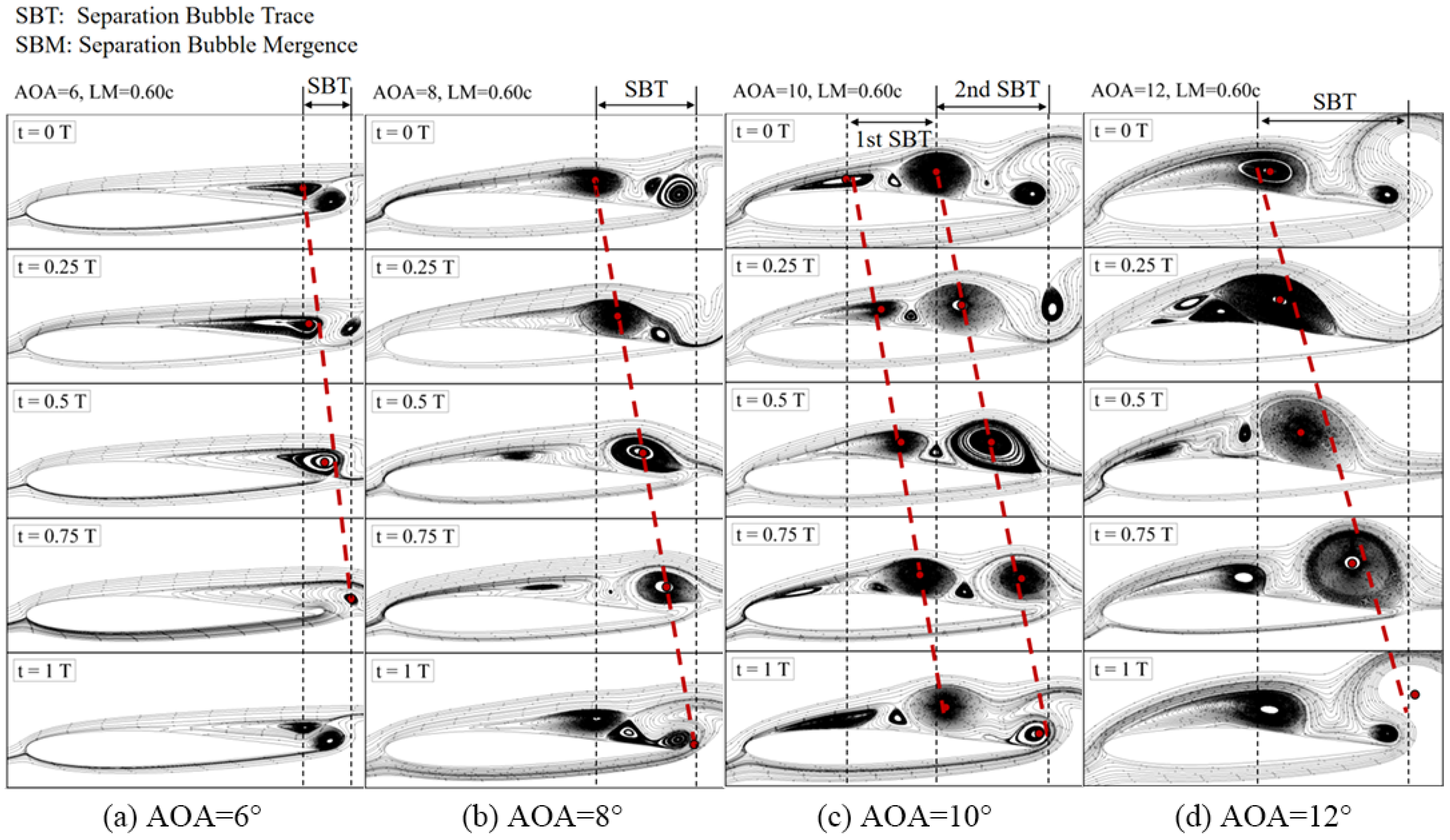
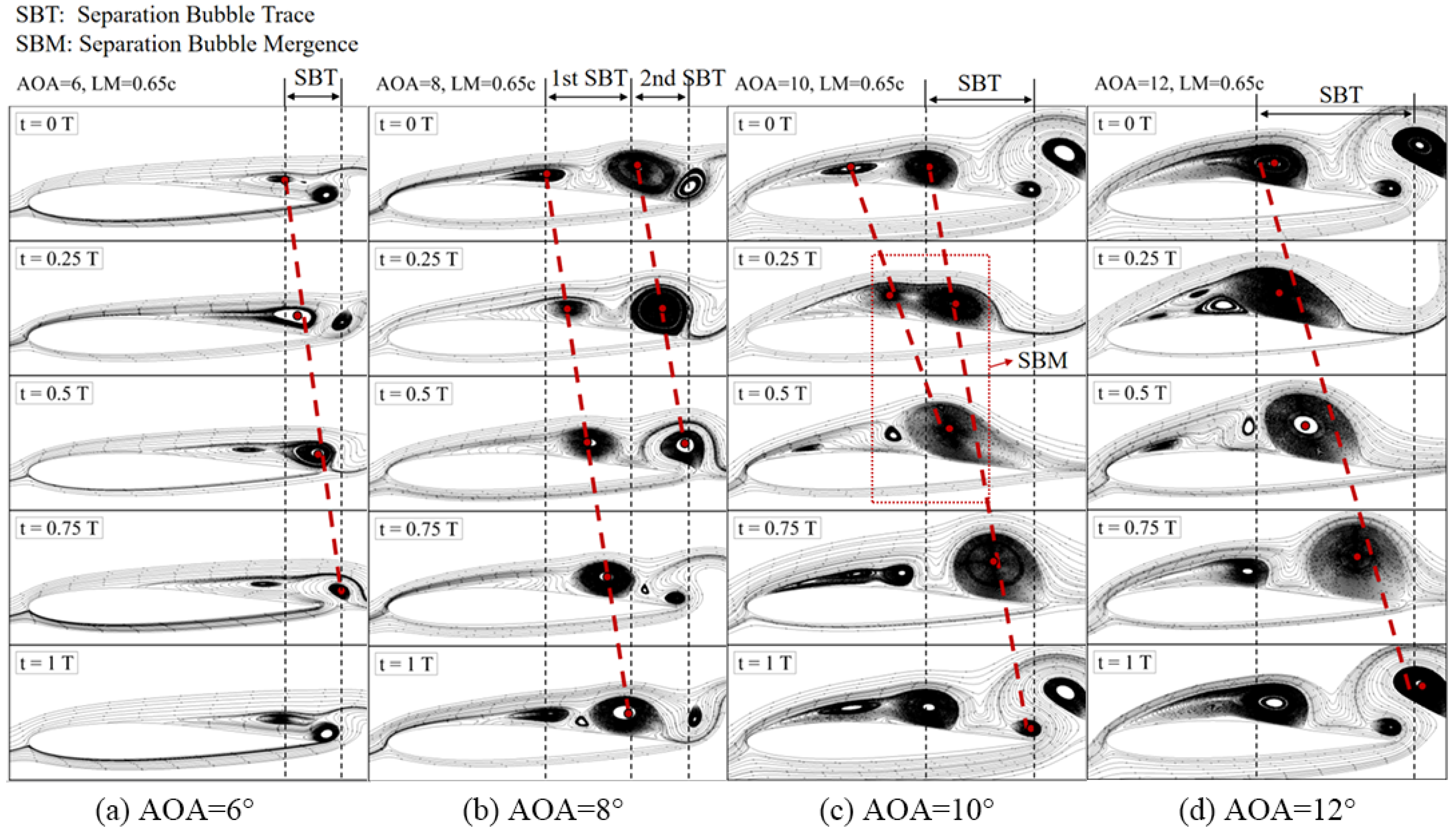
- Two spatial features of the unsteady flow are found to relate to the lift improvement. At AOA = 8°, more vortices, indicating more low-pressure regions, are observed on the upper surface of the membrane airfoil at LM = 0.65c compared to the case at LM = 0.60c. This result is consistent with the fact that the lift enhancement at LM = 0.65c (14.47%) is greater than that at LM = 0.60c(0.35%) at AOA = 8°. However, the number of vortices is not a decisive factor on the aerodynamic performance as the AOA increases to 10°. The lift enhancement at LM = 0.65c is about five times larger than that at LM = 0.60c while more vortices are observed at LM = 0.60c.
- (3)
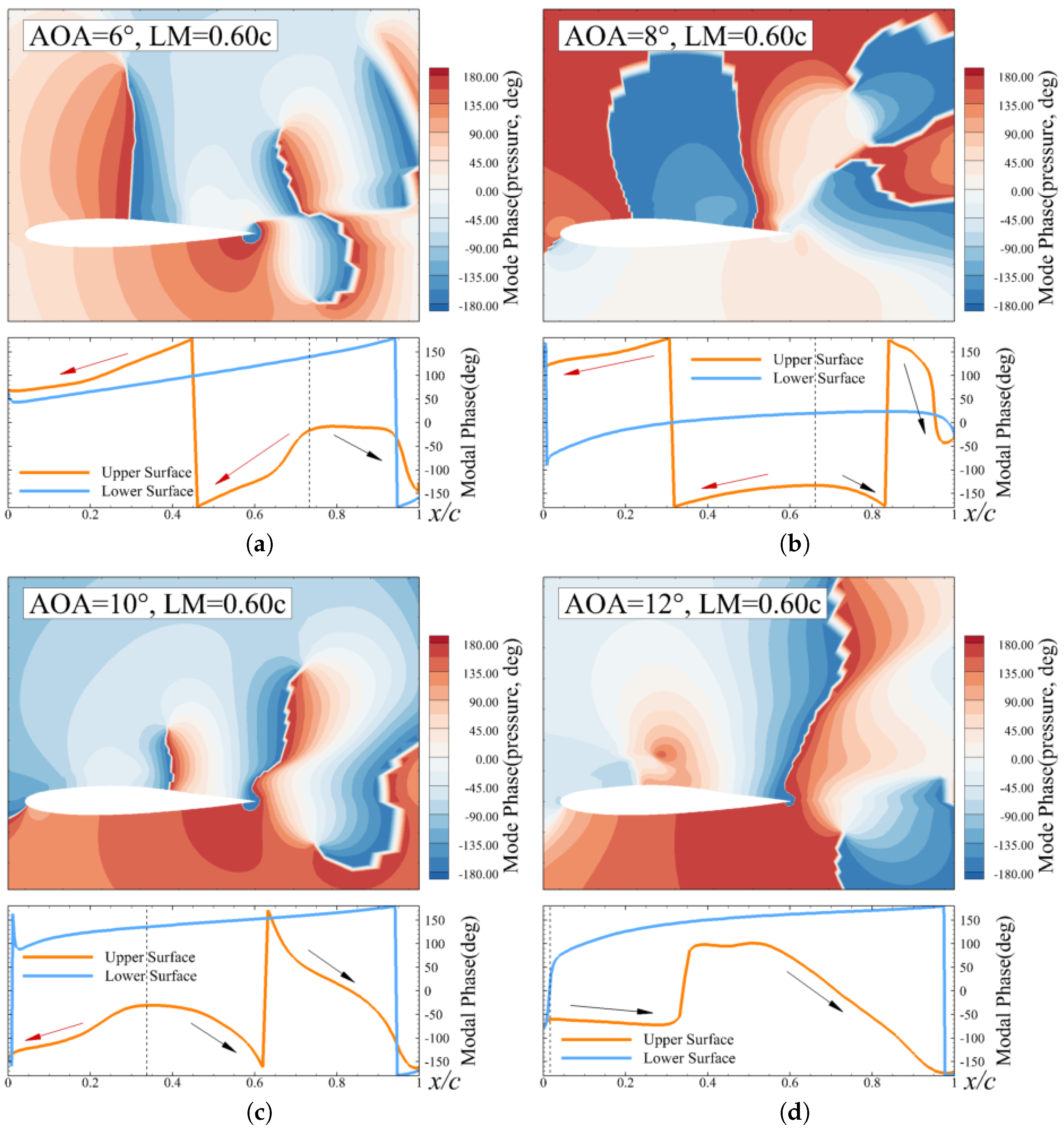
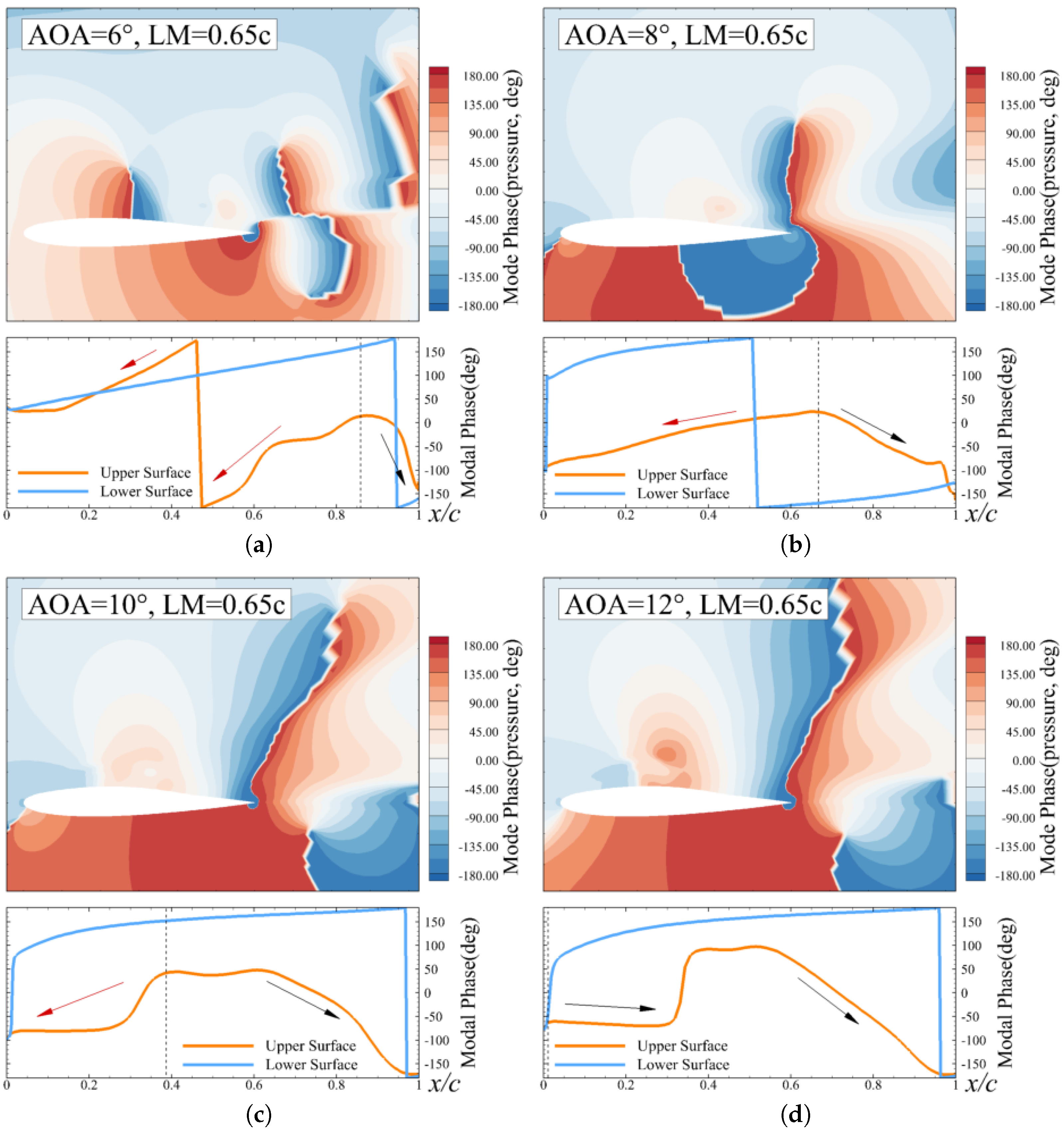
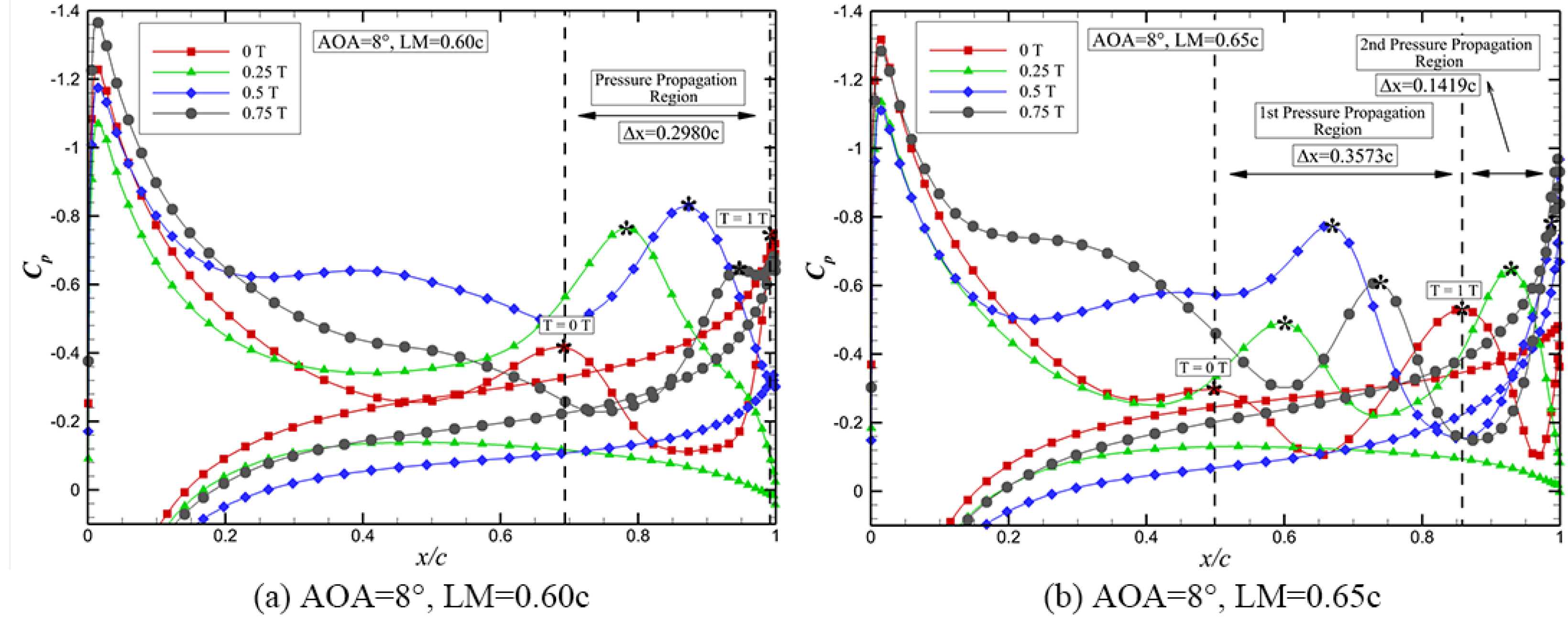
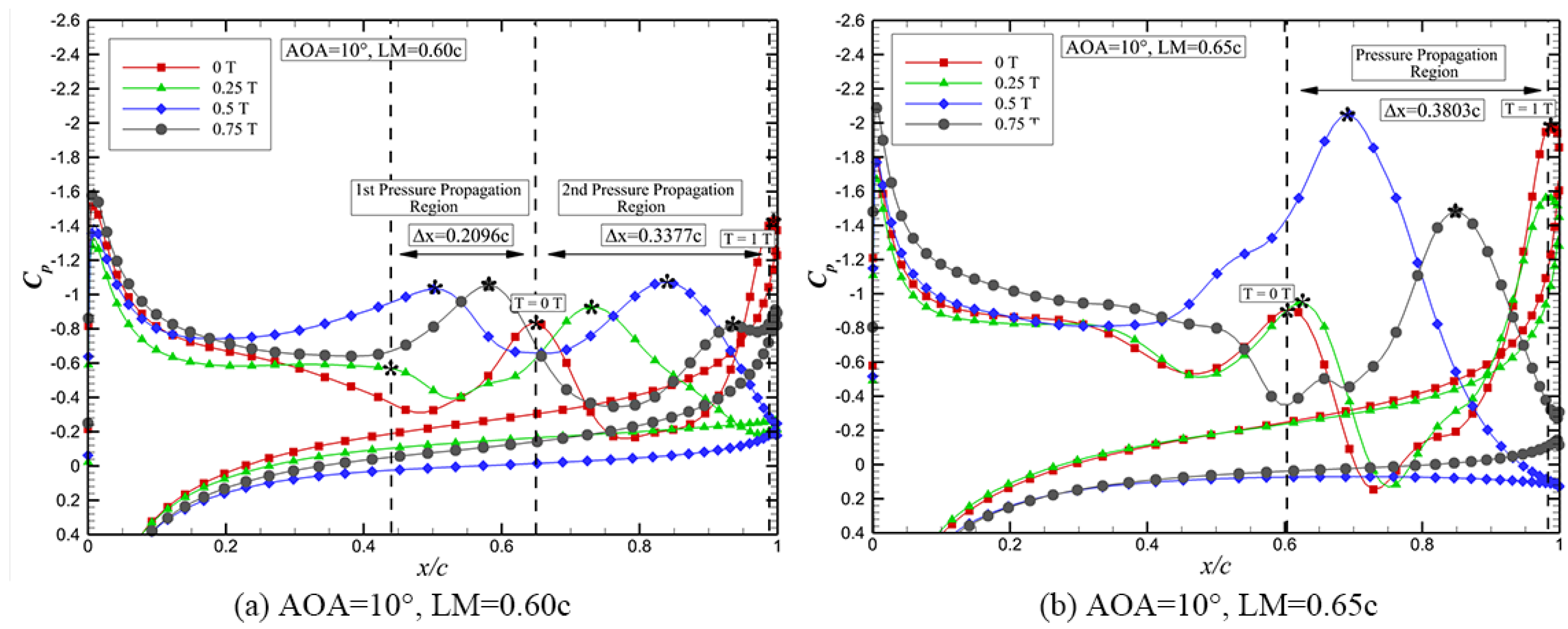
- The modal phase information based on DMD is used to identify the pressure propagation in the unsteady flow to study the coupling dynamics. Two kinds of pressure propagation region are identified on the upper surface of the membrane airfoil, i.e., the upstream pressure propagation (UPP) and the downstream pressure propagation (DPP). The boundary between the UPP and the DPP exhibits behavior similar to that of movement of the flow separation point, which suggests that the DPP region can serve as a key indicator for the physical interpretation of lift enhancement in the membrane airfoil.
- (4)
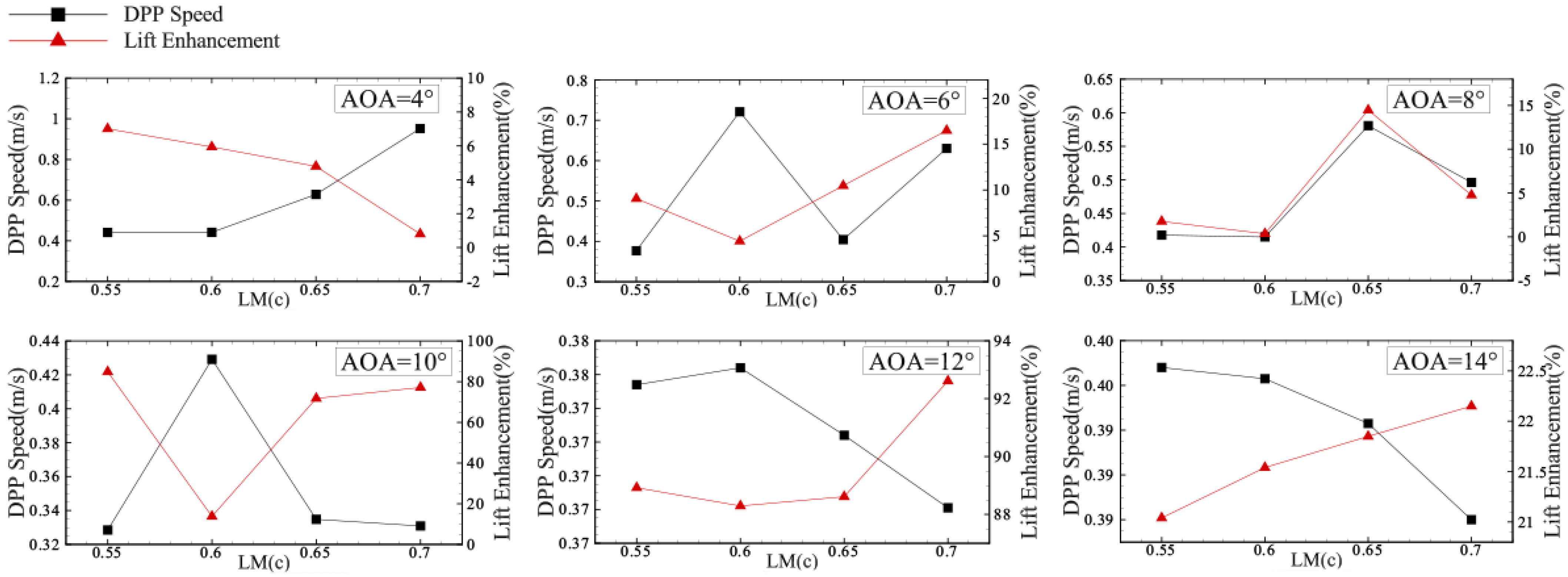
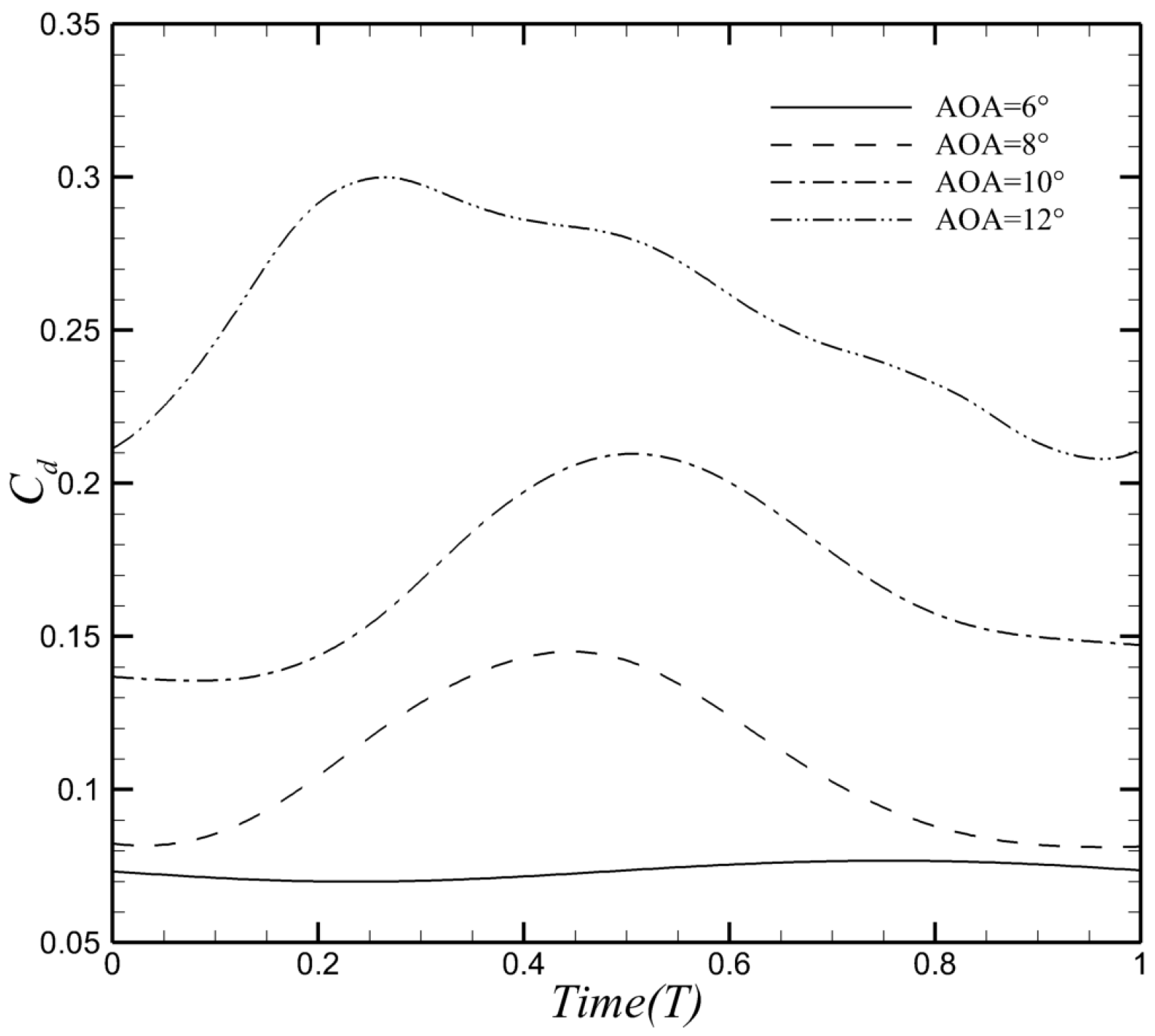
- The DPP speed is used to quantify the propagation speed of the lagged maximal pressure in the flow separation zone and unveil the relation between the evolution of the separation bubbles and the lift enhancement of the membrane airfoil. The lift, drag, lift–drag coefficients of the membrane airfoil at different AOAs and LMs are analyzed. The results show that two different mechanisms are found with opposite trend of the DPP speed with respect to the LMs. (I) The positive correlation between DPP speed and lift enhancement is found at AOA = 8°. The faster DPP induces more vortices, indicating more low-pressure regions at LM = 0.65c compared to the other cases, which lead to a higher lift enhancement. (II) An inverse relation between DPP speed and lift enhancement is found as the LM grows when the AOA exceeds 8°. In these cases, the separation bubbles are merged into a large-scale separation bubble. The lower DPP speed can maintain this large-scale separation bubble on the upper surface of the airfoil, which benefits the aerodynamic performance. The membrane airfoil investigated in this study is primarily applicable to low Reynolds number flows. In ongoing research, the flow control of locally flexible airfoil will aim for high Reynolds number flows. Furthermore, all the models in this study are two-dimensional. It will be worth exploring the three-dimensional flow structure induced by the coupling of the membrane structures.
Author Contributions
Funding
Data Availability Statement
Conflicts of Interest
References
- Tiomkin, S.; Raveh, D.E. A review of membrane-wing aeroelasticity. Prog. Aerosp. Sci. 2021, 126. [Google Scholar] [CrossRef]
- Smith, R.; Shyy, W. Computational model of flexible membrane wings in steady laminar flow. AIAA J. 1995, 33, 1769–1777. [Google Scholar] [CrossRef]
- Gordnier, R.E. High fidelity computational simulation of a membrane wing airfoil. J. Fluids Struct. 2009, 25, 897–917. [Google Scholar] [CrossRef]
- Molki, M.; Breuer, K. Oscillatory motions of a prestrained compliant membrane caused by fluid–membrane interaction. J. Fluids Struct. 2010, 26, 339–358. [Google Scholar] [CrossRef]
- Serrano-Galiano, S.; Sandham, N.D.; Sandberg, R.D. Fluid–structure coupling mechanism and its aerodynamic effect on membrane aerofoils. J. Fluid Mech. 2018, 848, 1127–1156. [Google Scholar] [CrossRef]
- Kang, W.; Zhang, J.Z.; Feng, P.H. Aerodynamic analysis of a localized flexible airfoil at low Reynolds numbers. Commun. Comput. Phys. 2012, 11, 1300–1310. [Google Scholar]
- Kang, W.; Zhang, J.Z.; Lei, P.F.; Xu, M. Computation of unsteady viscous flow around a locally flexible airfoil at low Reynolds number. J. Fluids Struct. 2014, 46, 42–58. [Google Scholar]
- Lei, P.F.; Zhang, J.Z.; Kang, W.; Ren, S.; Wang, L. Unsteady Flow Separation and High Performance of Airfoil with Local Flexible Structure at Low Reynolds Number. Commun. Comput. Phys. 2014, 16, 699–717. [Google Scholar] [CrossRef]
- Arif, I.; Lam, G.C.Y.; Wu, D.; Leung, R.C.K. Passive airfoil tonal noise reduction by localized flow-induced vibration of an elastic panel. Aerosp. Sci. Technol. 2020, 107, 106319. [Google Scholar] [CrossRef]
- Arif, I.; Lam, G.C.Y.; Leung, R.C.K. Coupled structural resonance of elastic panels for suppression of airfoil tonal noise. J. Fluids Struct. 2022, 110, 103506. [Google Scholar] [CrossRef]
- Sun, X.; Zhang, X.; Su, Z.; Huang, D. Experimental Study of Aerodynamic Characteristics of Partially Flexible NACA0012 Airfoil. AIAA J. 2022, 60, 5386–5400. [Google Scholar] [CrossRef]
- Song, A.; Tian, X.; Israeli, E.; Galvao, R.; Bishop, K.; Swartz, S.; Breuer, K. Aeromechanics of Membrane Wings with Implications for Animal Flight. AIAA J. 2008, 46, 2096–2106. [Google Scholar] [CrossRef]
- Rojratsirikul, P.; Wang, Z.; Gursul, I. Unsteady fluid–structure interactions of membrane airfoils at low Reynolds numbers. Exp. Fluids 2009, 46, 859–872. [Google Scholar] [CrossRef]
- Rojratsirikul, P.; Wang, Z.; Gursul, I. Effect of pre-strain and excess length on unsteady fluid–structure interactions of membrane airfoils. J. Fluids Struct. 2010, 26, 359–376. [Google Scholar] [CrossRef]
- Rojratsirikul, P.; Genc, M.S.; Wang, Z.; Gursul, I. Flow-induced vibrations of low aspect ratio rectangular membrane wings. J. Fluids Struct. 2011, 27, 1296–1309. [Google Scholar] [CrossRef]
- Açıkel, H.H.; Serdar Genç, M. Control of laminar separation bubble over wind turbine airfoil using partial flexibility on suction surface. Energy 2018, 165, 176–190. [Google Scholar] [CrossRef]
- Bleischwitz, R.; de Kat, R.; Ganapathisubramani, B. On the fluid-structure interaction of flexible membrane wings for MAVs in and out of ground-effect. J. Fluids Struct. 2017, 70, 214–234. [Google Scholar] [CrossRef]
- Abdolahipour, S. Review on flow separation control: Effects of excitation frequency and momentum coefficient. Front. Mech. Eng. 2024, 10, 1380675. [Google Scholar] [CrossRef]
- Shahrokhi, S.S.; Taeibi Rahni, M.; Akbari, P. Aerodynamic design of a double slotted morphed flap airfoil—A numerical study. Front. Mech. Eng. 2024, 10, 1371479. [Google Scholar] [CrossRef]
- Taleghani, A.S.; Hesabi, A.; Esfahanian, V. Numerical Study of Flow Control to Increase Vertical Tail Effectiveness of an Aircraft by Tangential Blowing. Int. J. Aeronaut. Space Sci. 2025, 26, 785–799. [Google Scholar] [CrossRef]
- Dong, Y.; Boming, Z.; Jun, L. A changeable aerofoil actuated by shape memory alloy springs. Mater. Sci. Eng. A 2008, 485, 243–250. [Google Scholar] [CrossRef]
- Bilgen, O.; Kochersberger, K.B.; Inman, D.J.; Ohanian, O.J. Novel, Bidirectional, Variable-Camber Airfoil via Macro-Fiber Composite Actuators. J. Aircr. 2010, 47, 303–314. [Google Scholar] [CrossRef]
- Hays, M.R.; Morton, J.; Oates, W.S.; Dickinson, B.T. Aerodynamic Control of Micro Air Vehicle Wings Using Electroactive Membranes. In Proceedings of the ASME 2011 Conference on Smart Materials, Adaptive Structures and Intelligent Systems, Scottsdale, AZ, USA, 18–21 September 2011; Volume 1, SMASIS2011-5076. pp. 583–591. [Google Scholar] [CrossRef]
- Gursul, I.; Cleaver, D.J.; Wang, Z. Control of low Reynolds number flows by means of fluid–structure interactions. Prog. Aerosp. Sci. 2014, 64, 17–55. [Google Scholar] [CrossRef]
- Tiomkin, S.; Raveh, D. On the stability of two-dimensional membrane wings. J. Fluids Struct. 2017, 71, 143–163. [Google Scholar] [CrossRef]
- Tiomkin, S.; Raveh, D.E. On membrane-wing stability in laminar flow. J. Fluids Struct. 2019, 91, 102694. [Google Scholar] [CrossRef]
- Li, G.; Jaiman, R.K.; Khoo, B.C. Flow-excited membrane instability at moderate Reynolds numbers. J. Fluid Mech. 2021, 929, A40. [Google Scholar] [CrossRef]
- He, X.; Wang, J.J. Fluid–structure interaction of a flexible membrane wing at a fixed angle of attack. Phys. Fluids 2020, 32, 127102. [Google Scholar] [CrossRef]
- Bohnker, J.R.; Breuer, K.S. Control of Separated Flow Using Actuated Compliant Membrane Wings. AIAA J. 2019, 57, 3801–3811. [Google Scholar] [CrossRef]
- Huang, G.; Xia, Y.; Dai, Y.; Yang, C.; Wu, Y. Fluid–structure interaction in piezoelectric energy harvesting of a membrane wing. Phys. Fluids 2021, 33, 063610. [Google Scholar] [CrossRef]
- Kang, W.; Xu, M.; Yao, W.; Zhang, J. Lock-in mechanism of flow over a low-Reynolds-number airfoil with morphing surface. Aerosp. Sci. Technol. 2020, 97, 105647. [Google Scholar] [CrossRef]
- Taira, K.; Brunton, S.L.; Dawson, S.T.M.; Rowley, C.W.; Colonius, T.; McKeon, B.J.; Schmidt, O.T.; Gordeyev, S.; Theofilis, V.; Ukeiley, L.S. Modal Analysis of Fluid Flows: An Overview. AIAA J. 2017, 55, 4013–4041. [Google Scholar] [CrossRef]
- Taira, K.; Hemati, M.S.; Brunton, S.L.; Sun, Y.; Duraisamy, K.; Bagheri, S.; Dawson, S.T.M.; Yeh, C.A. Modal Analysis of Fluid Flows: Applications and Outlook. AIAA J. 2020, 58, 998–1022. [Google Scholar] [CrossRef]
- Abdolahipour, S. Effects of low and high frequency actuation on aerodynamic performance of a supercritical airfoil. Front. Mech. Eng. 2023, 9, 1290074. [Google Scholar] [CrossRef]
- Schmid, P.J. Dynamic mode decomposition of numerical and experimental data. J. Fluid Mech. 2010, 656, 5–28. [Google Scholar] [CrossRef]
- Schmid, P.J. Dynamic Mode Decomposition and Its Variants. Annu. Rev. Fluid Mech. 2022, 54, 225–254. [Google Scholar] [CrossRef]
- Poplingher, L.; Raveh, D.E.; Dowell, E.H. Modal Analysis of Transonic Shock Buffet on 2D Airfoil. AIAA J. 2019, 57, 2851–2866. [Google Scholar] [CrossRef]
- Weiner, A.; Semaan, R. Robust Dynamic Mode Decomposition Methodology for an Airfoil Undergoing Transonic Shock Buffet. AIAA J. 2023, 61, 4456–4467. [Google Scholar] [CrossRef]
- Iyer, P.S.; Mahesh, K. A numerical study of shear layer characteristics of low-speed transverse jets. J. Fluid Mech. 2016, 790, 275–307. [Google Scholar] [CrossRef]
- Motheau, E.; Nicoud, F.; Poinsot, T. Mixed acoustic–entropy combustion instabilities in gas turbines. J. Fluid Mech. 2014, 749, 542–576. [Google Scholar] [CrossRef]
- Mohan, A.T.; Gaitonde, D.V. Analysis of Airfoil Stall Control Using Dynamic Mode Decomposition. J. Aircr. 2017, 54, 1508–1520. [Google Scholar] [CrossRef]
- Zhang, H.; Jia, L.; Fu, S.; Xiang, X.; Wang, L. Vortex shedding analysis of flows past forced-oscillation cylinder with dynamic mode decomposition. Phys. Fluids 2023, 35, 053618. [Google Scholar] [CrossRef]
- Rojratsirikul, P.; Wang, Z.; Gursul, I. Unsteady Aerodynamics of Membrane Airfoils. In Proceedings of the 46th AIAA Aerospace Sciences Meeting and Exhibit, Reno, NV, USA, 7–10 January 2008; pp. 1–20. [Google Scholar] [CrossRef]
- Kang, W.; Hu, S.; Wang, Y. Lift enhancement mechanism study of the airfoil with a dielectric elastic membrane skin. J. Fluids Struct. 2024, 125, 104083. [Google Scholar] [CrossRef]
- Sanchez, R.; Palacios, R.; Economon, T.D.; Kline, H.L.; Alonso, J.J.; Palacios, F. Towards a Fluid-Structure Interaction Solver for Problems with Large Deformations Within the Open-Source SU2 Suite. In Proceedings of the 57th AIAA/ASCE/AHS/ASC Structures, Structural Dynamics, and Materials Conference, San Diego, CA, USA, 4–8 January 2016. [Google Scholar] [CrossRef]
- Kang, W.; Chen, B.; Hu, S. Coupling Analysis between the Transonic Buffeting Flow and a Heaving Supercritical Airfoil Based on Dynamic Mode Decomposition. Aerospace 2024, 11, 722. [Google Scholar] [CrossRef]
- Buoso, S.; Palacios, R. Electro-aeromechanical modelling of actuated membrane wings. J. Fluids Struct. 2015, 58, 188–202. [Google Scholar] [CrossRef]
- Tissot, G.; Cordier, L.; Benard, N.; Noack, B.R. Model reduction using Dynamic Mode Decomposition. Comptes Rendus MéCanique 2014, 342, 410–416. [Google Scholar] [CrossRef]


| Structural Parameters | Value |
|---|---|
| Chord (c) | 300 mm |
| Length of membrane | 0.55c–0.70c |
| Thickness (t) | 0.2 mm |
| Elastic modulus (E) | 34,150 Pa |
| Structural density () | 402.3 kg/m3 |
| Pressure on the lower surface | 1 atm |
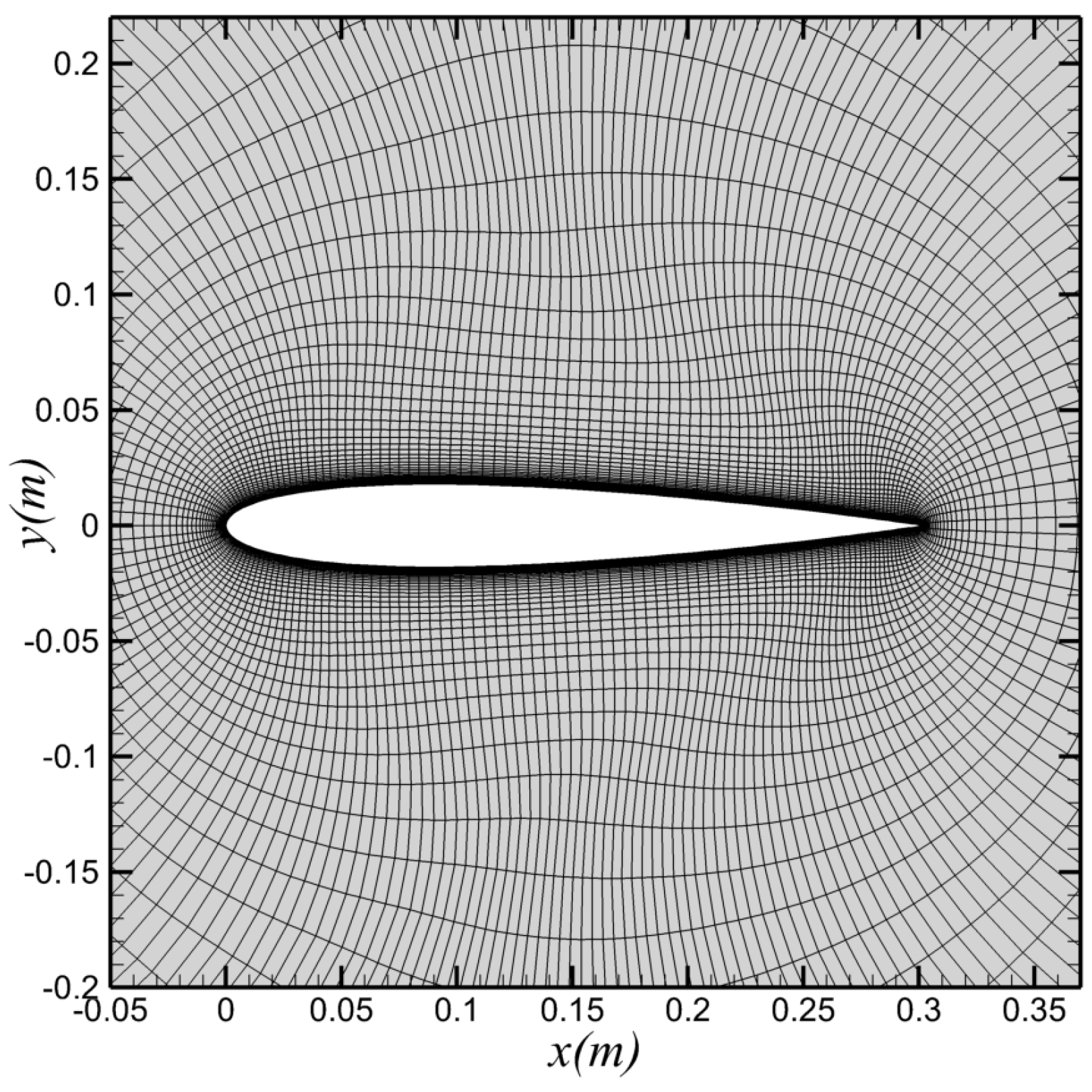
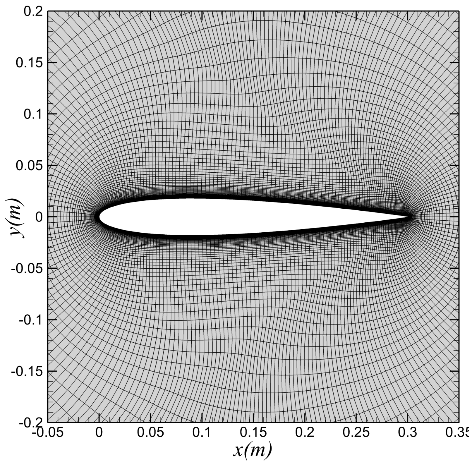
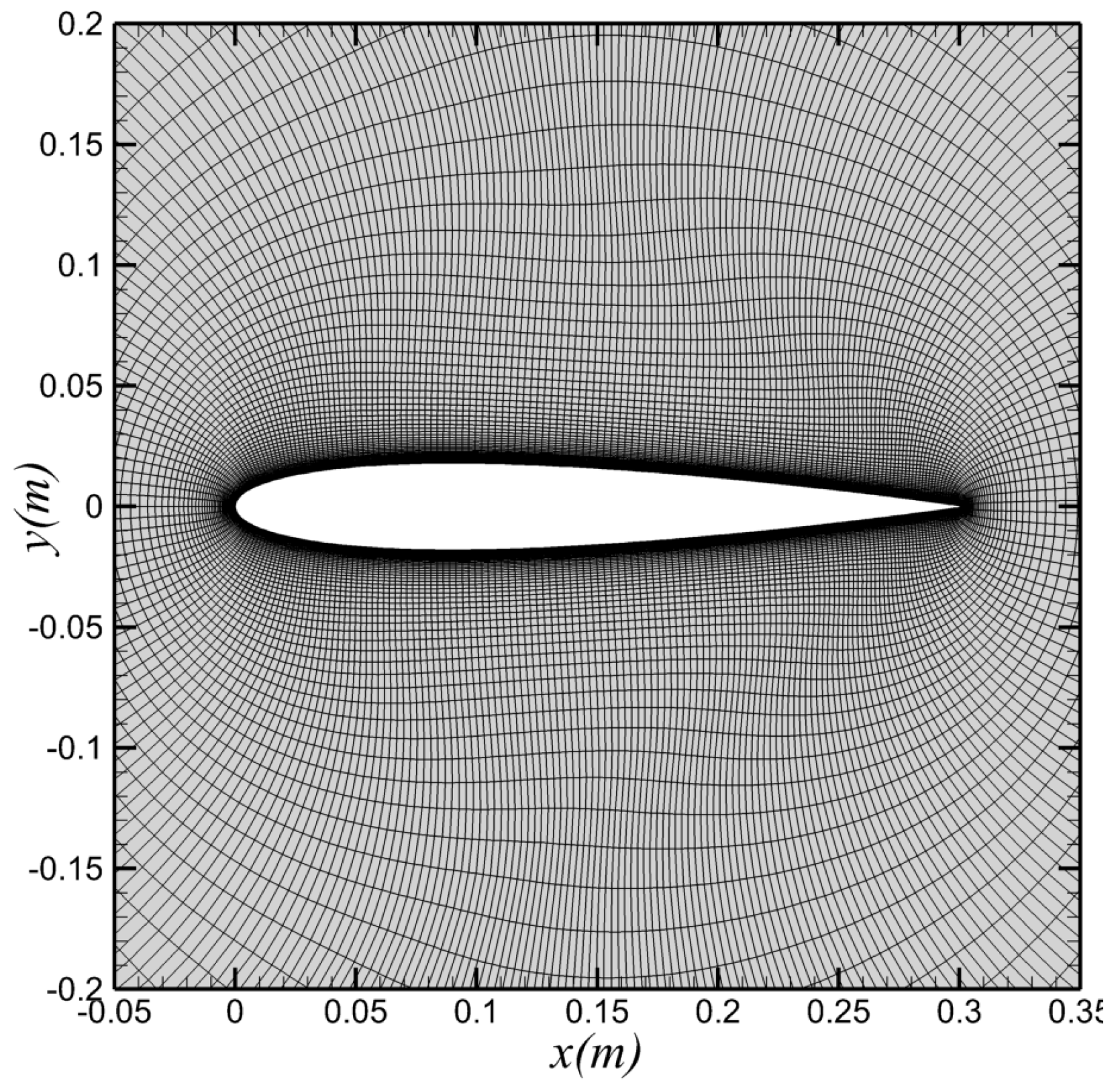
| Cases | Coarse-Size Grid | Middle-Size Grid | Fine-Size Grid |
|---|---|---|---|
| Grid size | 125 × 65 | 254 × 81 | 402 × 161 |
| Time-averaged lift coefficient | 0.5627 | 0.5919 | 0.5942 |
| 1st-order frequency of the flow | 3.50 | 3.40 | 3.40 |
| 1st-order frequency of the structure | 3.40 | 3.40 | 3.50 |
| Structural Parameters | Flow Parameters | ||
|---|---|---|---|
| Chord (c) | 136.6 mm | Freestream velocity | 1.0 m/s |
| Thickness (t) | 0.2 mm | Fluid density | 1.0 kg/m3 |
| Elastic modulus (E) | 34,150 Pa | Re | 2500 |
| Structural density () | 402.3 kg/m3 | Angle of attack | 4° |
Disclaimer/Publisher’s Note: The statements, opinions and data contained in all publications are solely those of the individual author(s) and contributor(s) and not of MDPI and/or the editor(s). MDPI and/or the editor(s) disclaim responsibility for any injury to people or property resulting from any ideas, methods, instructions or products referred to in the content. |
© 2025 by the authors. Licensee MDPI, Basel, Switzerland. This article is an open access article distributed under the terms and conditions of the Creative Commons Attribution (CC BY) license (https://creativecommons.org/licenses/by/4.0/).
Share and Cite
Kang, W.; Hu, S.; Chen, B.; Yao, W. Modal Phase Study on Lift Enhancement of a Locally Flexible Membrane Airfoil Using Dynamic Mode Decomposition. Aerospace 2025, 12, 313. https://doi.org/10.3390/aerospace12040313
Kang W, Hu S, Chen B, Yao W. Modal Phase Study on Lift Enhancement of a Locally Flexible Membrane Airfoil Using Dynamic Mode Decomposition. Aerospace. 2025; 12(4):313. https://doi.org/10.3390/aerospace12040313
Chicago/Turabian StyleKang, Wei, Shilin Hu, Bingzhou Chen, and Weigang Yao. 2025. "Modal Phase Study on Lift Enhancement of a Locally Flexible Membrane Airfoil Using Dynamic Mode Decomposition" Aerospace 12, no. 4: 313. https://doi.org/10.3390/aerospace12040313
APA StyleKang, W., Hu, S., Chen, B., & Yao, W. (2025). Modal Phase Study on Lift Enhancement of a Locally Flexible Membrane Airfoil Using Dynamic Mode Decomposition. Aerospace, 12(4), 313. https://doi.org/10.3390/aerospace12040313