Augmented Hohmann Transfer for Spacecraft with Continuous-Thrust Propulsion System

Abstract

Hohmann transfer is the classical approach used in astrodynamics to analyze the optimal bi-impulsive transfer, from the point of view of the total velocity change, between two circular, coplanar orbits of assigned radius. The Hohmann transfer is characterized by an elliptical trajectory tangent to both circular orbits at the points where the transfer begins or ends and can be used to simply model, in a Kepler problem, a possible optimal transfer of a spacecraft equipped with a high-thrust propulsion system. Recent literature has proposed a sort of extension of the Hohmann transfer to a heliocentric mission scenario, where the total velocity change is reduced compared to the classical result by employing a photonic solar sail operating along the deep-space transfer trajectory. The study of this so-called augmented Hohmann transfer, where the spacecraft uses both two tangential impulses (one at the beginning and one at the end of the flight) provided by a high-thrust propulsion system and the propulsive acceleration (during the flight) provided by a low-thrust propulsion system, is extended in this paper by considering a more general case where the spacecraft moves around a generic primary body and uses, along the transfer, a freely orientable propulsive acceleration vector with constant and assigned magnitude. This scenario is consistent, for example, with the use of a typical electric thruster instead of the photonic solar sail considered in recent literature. In particular, the paper studies the impact of the continuous-thrust propulsion system on the transfer performance between the two circular orbits, analyzing the variation of the total velocity change as a function of the propulsive acceleration magnitude. The procedure, which uses an optimal approach to performance estimation, can be used both in a heliocentric and planetocentric mission scenario and can also be employed to analyze the performance of a spacecraft equipped with a multimode propulsion system.

1. Introduction

The Hohmann transfer is probably the most famous two-impulse maneuver that allows the spacecraft transfer between two circular and coplanar orbits in an inverse-square gravitational field, as discussed by Gobetz and Doll in their classical review paper of 1969 [1]. On the other hand, the Hohmann transfer is certainly the first method described in basic astrodynamics courses as part of the multiple impulses orbital maneuvers for transferring a space vehicle equipped with a high-thrust propulsion system between two Keplerian trajectories [2,3,4,5]. This famous spacecraft transfer technique, as is well known, was proposed by the German engineer Walter Hohmann in their pioneering work published in October 1925 [6], and it is characterized by the use of an elliptical transfer orbit tangent, at the periapsis and apoapsis points, to the two circular and coplanar orbits involved in the problem.

A simplified scheme of the classical Hohmann transfer (indicated with acronym CHT in the text, and with the subscript H in the mathematical model) is shown in Figure 1, which illustrates the two possible cases of an orbit raising, i.e., the case of a final circular orbit with radius $r_f$ greater than that ($r_i$) of the starting orbit, or of an orbit lowering where $r_f<r_i$. In particular, Figure 1 also indicates the direction of the two velocity changes related to the two impulsive maneuvers that allow the spacecraft to move from the initial circular orbit to the transfer orbit ($\Delta v_{i_H}$), and from the transfer orbit to the final circular orbit ($\Delta v_{f_H}$). As is well known, these are tangential impulsive maneuvers which are indicated through two green arrows in the simplified scheme of Figure 1, i.e., directed exactly along the local velocity vector of the spacecraft.

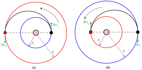
Figure 1. Sketch of the CHT between an initial circular orbit of radius $r_i$ and a final circular orbit of radius $r_f$. All orbits are traversed in a counterclockwise direction. Black line → CHT trajectory; blue line → initial circular orbit; red line → final circular orbit; black dot → first impulsive maneuver; red square → second impulsive maneuver; pink circle → primary body. (a) Case of an orbit raising with $r_f>r_i$. (b) Case of an orbit lowering with $r_f<r_i$.

The importance of the CHT lies not only in the elegance and simplicity with which this spacecraft maneuver can be studied analytically and geometrically without the aid of complex (and sometimes long) numerical simulations [7], but above all in the fact that, among all the bi-impulsive spacecraft maneuvers, it is the one that allows to minimize the total velocity change $\Delta v_H=\Delta v_{i_H}+\Delta v_{f_H}$ required to complete the transfer between the two (coplanar) circular orbits of assigned characteristics [8,9]. In this sense, the proof of the optimality of the CHT can be found in several bibliographic sources, starting from Lawden’s treatment based on calculus of variations [10], passing through Palmore’s simple and effective approach based on gradient method and ordinary calculus [11], to arrive for example at the elegant geometric model proposed by Prussing in 1992 [12] or the graphical approach discussed more recently by Pontani [13].

For a given primary body and in a given mission scenario defined by the pair of orbital radii $\{r_i,r_f\}$, the analytical results provided by Walter Hohmann—the interested reader may appreciate, in this regard, the elegant discussion reported in chapter 4 of Ref. [6]—allow to uniquely determine the total velocity change $\Delta v_H$, the flight time $\Delta t_H$, and the angle $\Delta {\theta }_H\triangleq \pi \mathrm{rad}$ traveled by the spacecraft during the transfer, as briefly summarized in Section 2. However, for a given pair $\{r_i,r_f\}$, the total velocity change can be further reduced with respect to the value $\Delta v_H$ obtainable in the CHT, while maintaining the same value of flight time and center angle swept by the spacecraft, by employing an additional, continuous-thrust, propulsion system acting during the flight phase between the two tangential impulsive maneuvers. This sort of Augmented Hohmann Transfer (indicated with the acronym AHT in the text, and with the subscript A in the mathematical model) has been recently studied by the author of [14] in the interesting case in which the continuous-thrust propulsion system installed onboard the spacecraft is a typical photonic solar sail [15,16]. The latter is a propellantless propulsion system that uses solar radiation pressure to produce continuous propulsive acceleration by exploiting a large, highly reflective surface, essentially as if it were an extremely light mirror in orbit around the primary body [17,18]. However, the physics involved in generating propulsive force by a solar sail do not allow the thrust vector to be freely directed in space, since this vector is strictly tied to the orientation of the nominal plane of the reflecting membrane with respect to the Sun–spacecraft direction [19,20].

The aim of this paper is, therefore, to analyze the performance of an AHT in the general case in which the additional propulsion system installed onboard the spacecraft is able to give, during the flight between the two tangential impulsive maneuvers, a freely steerable propulsive acceleration vector ${\mathit{a}}_p$ of constant and assigned magnitude $a_p=\parallel {\mathit{a}}_p\parallel$. This scenario is a possible approximation of the actual behavior of a typical solar electric thruster [21,22], in which the thrust level is varied during the orbital transfer as a function of the mass change due to the propellant consumption, in such a way as to obtain a constant value of $a_p$. In fact, this sort of ideal thruster which is able to give a freely steerable propulsive acceleration vector of constant magnitude has been widely used in the literature, starting from the pioneering work by Tsien [23] on the escape trajectories of a spacecraft with a radial outward thrust, or the works by Boltz [24,25] in a substantially similar mission scenario. More recently, the same propulsion system concept has been used in Ref. [26] to evaluate analytically an accurate estimation of the solution of the two-point boundary value problem in an optimization process of a typical two-dimensional orbit transfer.

In this paper, the propulsive acceleration vector given by the additional propulsion system is used to reduce the total velocity change required by the two impulsive maneuvers with respect to the value achieved in a CHT. To this end, the problem is treated from an optimization point of view, in analogy with the approach used in Ref. [14]. However, in this case, the peculiar characteristics of the thrust vector ${\mathit{a}}_p$ do not allow to adapt the results obtained in the recent literature and require a new study of the problem and a new mathematical model for the determination of the optimal performances, as detailed in Section 3. The results of the numerical simulations, illustrated and discussed in Section 4, can be considered as a sort of intermediate step towards obtaining a performance model concerning an actual solar electric propulsion system, in which also the effect of the inevitable propellant consumption in reducing the total velocity change of the two impulsive maneuvers is taken into account. In fact, the presence inside an AHT of both (two) impulsive maneuvers and of an arc with continuous-thrust leads to consider such potential transfer maneuver as potentially obtainable by a spacecraft equipped with a hybrid thruster [27,28]; for example, a chemical–electric propulsion system whose potentialities have been recently explored in the context of a mission towards Mars [29,30,31].

The numerical results shown in Section 4 are obtained using a dimensionless form of the spacecraft dynamics, so that they can be used in a wide range of mission scenarios, including both planetocentric and heliocentric transfers. In this sense, Section 5 illustrates a set of specific applications of the general results, by considering a simplified form of some important mission scenarios as the low-Earth orbit raising or the interplanetary transfer towards Venus or Mars. In these mission scenarios, the trajectory optimization results are used to evaluate the impact of the presence of a continuous-thrust propulsion system on the total velocity change due to the tangential impulsive maneuvers, thus creating the necessary database to determine the effect of real thrusters on mission performance from the point of view of the propellant consumption. The latter will be the subject of future works, as indicated in Section 6, which concludes the paper.

2. Mathematical Preliminaries Regarding the CHT

This section briefly recalls the analytical mathematical model that describes, as a function of the geometric characteristics of the two coplanar circular orbits that appear in the problem, the performances of a CHT in terms of impulsive velocity changes ($\Delta v_{i_H}$ and $\Delta v_{f_H}$) and the total flight time ($\Delta t_H$). The procedure by which these well-known analytical relations are derived can be found in the fundamental texts of spaceflight mechanics [2,3,4,5], to which the interested reader is referred for any further information and comments.

Using fairly standard astrodynamic formulas [32,33], it is possible to write in a compact form the expressions of the two velocity changes $\{\Delta v_{i_H},\Delta v_{f_H}\}$ of the CHT as a function of the orbital radii $\{r_i,r_f\}$ and of the gravitational parameter $\mu$ of the generic primary body around which the transfer occurs. The results are as follows

$$\begin{array}{cc}\hfill \Delta v_{i_H}& =\sqrt{{\displaystyle \frac{\mu }{r_i}}}\left|\sqrt{{\displaystyle \frac{2r_f}{r_i+r_f}}}-1\right|\hfill \end{array}$$

(1)

$$\begin{array}{cc}\hfill \Delta v_{f_H}& =\sqrt{{\displaystyle \frac{\mu }{r_f}}}\left|1-\sqrt{{\displaystyle \frac{2r_i}{r_i+r_f}}}\right|\hfill \end{array}$$

(2)

which give the minimum value of the total velocity change $\Delta v_H$ of the CHT as

$$\Delta v_H=\Delta v_{i_H}+\Delta v_{f_H}\equiv \sqrt{{\displaystyle \frac{\mu }{r_i}}}\left[\left|\sqrt{{\displaystyle \frac{2\rho }{1+\rho }}}-1\right|+\sqrt{{\displaystyle \frac{1}{\rho }}}\left|1-\sqrt{{\displaystyle \frac{2}{1+\rho }}}\right|\right]$$

(3)

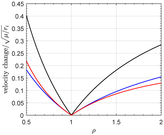
where $\rho \ne 1$ is a dimensionless (mission) design positive parameter that coincides with the ratio between the radius of the final orbit and that of the initial orbit, i.e., $\rho \triangleq r_f/r_i$. Equations (1)–(3) can be used to obtain the variation of the dimensionless form of the velocity changes $\{\Delta v_{i_H},\Delta v_{f_H},\Delta v_H\}$ as a function of $\rho$. In this case, the graphs obtained are summarized in Figure 2, which show that doubling the initial orbit radius trough a CHT requires a total velocity change of about $28\%$ of the orbital velocity magnitude along the parking circular orbit (i.e., $\sqrt{\mu /r_i}$), while halving $r_i$ requires about $40\%$ of $\sqrt{\mu /r_i}$.

Figure 2. Dimensionless form of the velocity change in a CHT as a function of the mission design parameter $\rho =r_f/r_i\ne 1$; see also Equations (1)–(3). Blue line → first impulse’s velocity change $\Delta v_{i_H}$; red line → second impulse’s velocity change $\Delta v_{f_H}$; black line → total velocity change $\Delta v_H$.

The expression of the total velocity change $\Delta v_H$ given by Equation (3) can be substituted in the rocket equation [32,33] to obtain the ratio $m_f/m_i$, where $m_i$ is the mass of the spacecraft just before the first impulsive maneuver, while $m_f$ is the spacecraft mass just after the second (and last) impulsive maneuver. In this regard, indicating with $u_h$ the exhaust velocity of the high-thrust propulsion system, that is, the thruster which is used to obtain the two impulsive maneuvers, the rocket equation [32,33] gives the following

$${\displaystyle \frac{m_{f_H}}{m_{i_H}}}\triangleq M_H=exp\left(-{\displaystyle \frac{\Delta v_H}{u_h}}\right)\equiv exp\left({\displaystyle \frac{-\left|\sqrt{\frac{2\rho }{1+\rho }}-1\right|-\sqrt{\frac{1}{\rho }}\left|1-\sqrt{\frac{2}{1+\rho }}\right|}{u_h/\sqrt{\mu /r_i}}}\right)$$

(4)

The contour plot of the function $M_H=M_H(\rho ,u_h/\sqrt{\mu /r_i})$ given by the previous equation is shown in Figure 3 for $\rho \in [0.5,2]$ and $u_h/\sqrt{\mu /r_i}\in [0.1,0.8]$.

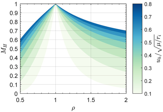
Figure 3. Dimensionless spacecraft mass ratio $M_H=m_{f_H}/m_{i_H}$ in a CHT as a function of $\rho \ne 1$; see also Equation (4).

On the other hand, the dimensionless parameter $\rho$ can also be used to express the time of flight $\Delta t_H$ of the transfer. The latter coincides with the orbital half-period of the elliptical CHT orbit (recall that the swept angle during the transfer is $\Delta \theta =\pi$ rad), which can be written as

$$\Delta t_H=\pi \sqrt{{\displaystyle \frac{r_i^3}{\mu }}}\sqrt{{\displaystyle \frac{{(1+\rho )}^3}{8}}}$$

(5)

This time of flight is drawn, in dimensionless form, in Figure 4.

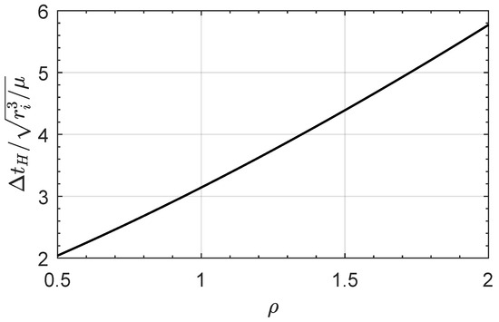
Figure 4. Transfer time $\Delta t_H$ in a CHT as a function of the dimensionless design parameter $\rho \ne 1$.

The analytical results summarized in this section will be used as a comparison to evaluate the effect of the presence of an additional continuous-thrust propulsion system acting during flight, whose mathematical modeling is described in Section 3.

3. Optimal Performance Evaluation in an Assigned AHT

This section illustrates the mathematical model used to analyze the optimal performance in an assigned AHT. More precisely, the AHT-based mission scenario is defined by the given pair $\{r_i,r_f\}$ of the circular orbits’ radii, the total flight time which coincides with that obtained in a CHT, and the total angle swept by the spacecraft during the transfer, which is again equal to the value obtained in a CHT, i.e., $\pi$ rad. In other terms, the AHT is studied by fixing the initial radial distance $r_i$, the final radial distance $r_f$, the flight time $\Delta t_H=\Delta t_H(r_i,r_f)$ given by Equation (5), and the polar angle change $\Delta {\theta }_H=\pi$ rad.

For a given value of the magnitude of the (constant) propulsive acceleration due to the continuous-thrust propulsion system, the direction of ${\mathit{a}}_p$ is then selected to minimize the sum of the velocity changes required by the first and second (tangential) impulsive maneuvers. In this context, the value of the magnitude $a_p$ must be carefully selected, since a too high value of $a_p$ results in a zero value of the two impulsive velocity changes, since in that case, the circle-to-circle two-dimensional transfer can be performed, with that value of the flight time and with that swept angle, using only the continuous-thrust propulsion system. For this reason, it is necessary to preliminarily determine the minimum value of $a_p$, indicated below with $a_p^{★}$, which allows to perform the assigned transfer without any impulsive maneuver. Once $a_p^{★}=a_p^{★}(r_i,r_f)$ has been determined, the value of $a_p$ in the generic AHT must be selected respecting the following condition

$$a_p\le a_p^{★}$$

(6)

in order to ensure the presence of the impulsive maneuvers in the transfer.

Accordingly, this section is divided into three parts. The first shows the equations of motion used to study the dynamics of the spacecraft in the two-dimensional mission scenario. In the second part, the value of $a_p^{★}$ is determined as a function of the dimensionless design parameter $\rho$ by solving a suitable optimization problem. Finally, taking into account the constraint given by Equation (6), the third part describes the analytical procedure used to set up the optimal control problem through which the connection between the minimum (impulsive) total velocity change required by the AHT and the characteristics of the additional propulsion system $a_p$ is investigated.

3.1. Spacecraft Two-Dimensional Dynamics in a Dimensionless Form

Consider the case of an AHT in which the spacecraft uses, between the two tangential impulsive maneuvers, an additional thruster capable of providing a propulsive acceleration vector ${\mathit{a}}_p$ having a constant and assigned magnitude $a_p$. In this two-dimensional mission scenario, the direction of ${\mathit{a}}_p$ is identified by the typical thrust angle $\alpha \in [-\pi ,\pi ]$ rad, which is defined as the angle between the direction of the propulsive acceleration vector and the radial line connecting the primary body and the spacecraft. In particular, $\alpha >0$ when the projection of ${\mathit{a}}_p$ along the direction of the spacecraft velocity vector is positive.

The spacecraft dynamics is analyzed in a typical polar reference frame $\mathcal{T}(O;r,\theta )$ with the origin O in the center of mass of the primary body, in which the polar angle $\theta$ is measured counterclockwise from the primary-spacecraft line at the beginning of the flight, that is, at the point in which the first impulsive maneuver occurs. In this reference frame, introduce the following dimensionless terms

$$\tilde{r}={\displaystyle \frac{r}{r_i}},{\tilde{v}}_r={\displaystyle \frac{v_r}{\sqrt{\mu /r_i}}},{\tilde{v}}_{\theta }={\displaystyle \frac{v_{\theta }}{\sqrt{\mu /r_i}}},\tilde{t}={\displaystyle \frac{t}{\sqrt{r_i^3/\mu }}},{\tilde{a}}_p={\displaystyle \frac{a_p}{\mu /r_i^2}}$$

(7)

where $v_r$ is the radial component of the spacecraft velocity vector, $v_{\theta }$ is the transverse component of the spacecraft velocity vector, and t is the time.

Accordingly, the dimensionless form of the spacecraft equations of motion are as follows

$${\tilde{r}}^{\prime }={\tilde{v}}_r,{\theta }^{\prime }={\displaystyle \frac{{\tilde{v}}_{\theta }}{\tilde{r}}},{\tilde{v}}_r^{\prime }={\displaystyle \frac{{\tilde{v}}_{\theta }^2}{\tilde{r}}}-{\displaystyle \frac{1}{{\tilde{r}}^2}}+{\tilde{a}}_{p}cos\alpha ,{\tilde{v}}_{\theta }^{\prime }=-{\displaystyle \frac{{\tilde{v}}_r{\tilde{v}}_{\theta }}{\tilde{r}}}+{\tilde{a}}_{p}sin\alpha$$

(8)

where the prime symbol indicates the derivative with respect to the dimensionless time $\tilde{t}$ defined in Equation (7). Bearing in mind that the first tangential impulsive maneuver alters only the magnitude of the spacecraft velocity, just after that impulse (dimensionless time $\tilde{t}={\tilde{t}}_0=0$), the state variables of the vehicle are given by

$$\tilde{r}\left({\tilde{t}}_0\right)=1,\theta \left({\tilde{t}}_0\right)=0,{\tilde{v}}_r\left({\tilde{t}}_0\right)=0,{\tilde{v}}_{\theta }\left({\tilde{t}}_0\right)={\tilde{v}}_{{\theta }_i}$$

(9)

where the value of ${\tilde{v}}_{{\theta }_i}$ coincides with the spacecraft velocity magnitude just after the first impulsive maneuver. Therefore, the dimensionless form of the (first) velocity change $\Delta v_{i_A}$ is given by

$${\widetilde{\Delta v}}_{i_A}\triangleq {\displaystyle \frac{\Delta v_{i_A}}{\sqrt{\mu /r_i}}}=\left|{\tilde{v}}_{{\theta }_i}-1\right|$$

(10)

in which ${\tilde{v}}_{{\theta }_i}$ represents one of the unknowns to be determined in order to minimize the total velocity change of the two impulsive maneuvers in the AHT.

Bearing in mind Equation (5), just before the second impulsive maneuver, that is, at the dimensionless time instant ${\tilde{t}}_f$ given by

$${\tilde{t}}_f={\displaystyle \frac{\Delta t_H}{\sqrt{r_i^3/\mu }}}=\pi \sqrt{{\displaystyle \frac{{(1+\rho )}^3}{8}}}$$

(11)

the spacecraft states are constrained by the following (final) conditions

$$\tilde{r}\left({\tilde{t}}_f\right)=\rho ,\theta \left({\tilde{t}}_f\right)=\Delta {\theta }_H\equiv \pi \mathrm{rad},{\tilde{v}}_r\left({\tilde{t}}_f\right)=0,{\tilde{v}}_{\theta }\left({\tilde{t}}_f\right)={\tilde{v}}_{{\theta }_f}$$

(12)

where ${\tilde{v}}_{{\theta }_f}$ is the transverse component of the spacecraft velocity vector just before the last impulsive maneuver. In fact, the (dimensionless) velocity change of this second impulse is simply given by

$${\widetilde{\Delta v}}_{f_A}\triangleq {\displaystyle \frac{\Delta v_{f_A}}{\sqrt{\mu /r_i}}}={\displaystyle \frac{|v_{{\theta }_f}-\sqrt{\mu /r_f}|}{\sqrt{\mu /r_i}}}\equiv \left|{\tilde{v}}_{{\theta }_f}-\sqrt{1/\rho }\right|$$

(13)

in which, again, ${\tilde{v}}_{{\theta }_f}$ is determined in order to minimize the total velocity change whose dimensionless form is as follows

$${\widetilde{\Delta v}}_A\triangleq {\displaystyle \frac{\Delta v_A}{\sqrt{\mu /r_i}}}={\widetilde{\Delta v}}_{i_A}+{\widetilde{\Delta v}}_{f_A}$$

(14)

Note that the dimensionless equations of motion (8) and the boundary conditions given by Equations (9) and (12) depend only on the two dimensionless parameters $\rho$ and ${\tilde{a}}_p$.

Minimization of ${\widetilde{\Delta v}}_A$ can be achieved by selecting a suitable control law of the thrust angle $\alpha$ during the transfer. However, before determining and numerically simulating the effect of such an optimal control law on the value of the total velocity change, it is necessary to determine the value of $a_p^{★}$ which places an upper limit on the value of the propulsive acceleration that can be used in the equations of motion (8), according to the constraint defined in Equation (6). This aspect of the problem is investigated in the Section 3.2.

3.2. Calculation of the Reference Value $a_p^{★}$

The minimum value of the propulsive acceleration magnitude given by the continuous-thrust propulsion system is obtained using an optimization approach in which the performance index

$$J_a\triangleq -{\tilde{a}}_p$$

(15)

is maximized for a given value of the dimensionless design parameter $\rho$. In this limit scenario, the spacecraft performs the orbital transfer without employing the two tangential impulsive maneuvers, so that the mathematical boundary conditions are substantially coincident with those given in Equations (9) and (12), with the exception of the equations involving the transverse velocity component ${\tilde{v}}_{\theta }$, which now become the following

$${\tilde{v}}_{\theta }\left({\tilde{t}}_0\right)=1,{\tilde{v}}_{\theta }\left({\tilde{t}}_f\right)={\displaystyle \frac{1}{\sqrt{\rho }}}$$

(16)

The maximization of the performance index $J_a$ is obtained using the calculus of variations [34,35,36]. In particular, bearing in mind that ${\tilde{a}}_p$ is a constant of motion, the set of dimensionless variables $\{{\lambda }_r,{\lambda }_{\theta },{\lambda }_{v_r},{\lambda }_{v_{\theta }},{\lambda }_{a_p}\}$ is introduced in order to obtain the dimensionless Hamiltonian function

$$\mathcal{H}={\lambda }_r{\tilde{v}}_r+{\displaystyle \frac{{\lambda }_{\theta }{\tilde{v}}_{\theta }}{\tilde{r}}}+{\lambda }_{v_r}\left({\displaystyle \frac{{\tilde{v}}_{\theta }^2}{\tilde{r}}}-{\displaystyle \frac{1}{{\tilde{r}}^2}}+{\tilde{a}}_{p}cos\alpha \right)+{\lambda }_{v_{\theta }}\left(-{\displaystyle \frac{{\tilde{v}}_r{\tilde{v}}_{\theta }}{\tilde{r}}}+{\tilde{a}}_{p}sin\alpha \right)$$

(17)

and the Euler–Lagrange equations

$$\begin{array}{cc}\hfill {\lambda }_r^{\prime }& =-{\displaystyle \frac{{\lambda }_{v_r}\left(2-\tilde{r}{\tilde{v}}_{\theta }^2\right)-{\lambda }_{\theta }\tilde{r}{\tilde{v}}_{\theta }+{\lambda }_{v_{\theta }}\tilde{r}{\tilde{v}}_r{\tilde{v}}_{\theta }}{{\tilde{r}}^3}}\hfill \end{array}$$

(18)

$$\begin{array}{cc}\hfill {\lambda }_{\theta }^{\prime }& =0\hfill \end{array}$$

(19)

$$\begin{array}{cc}\hfill {\lambda }_{v_r}^{\prime }& ={\displaystyle \frac{{\lambda }_{v_{\theta }}{\tilde{v}}_{\theta }}{\tilde{r}}}-{\lambda }_r\hfill \end{array}$$

(20)

$$\begin{array}{cc}\hfill {\lambda }_{v_{\theta }}^{\prime }& =-{\displaystyle \frac{{\lambda }_{\theta }-{\lambda }_{v_{\theta }}{\tilde{v}}_r+2{\lambda }_{v_r}{\tilde{v}}_{\theta }}{\tilde{r}}}\hfill \end{array}$$

(21)

$$\begin{array}{cc}\hfill {\lambda }_{a_p}^{\prime }& =-{\lambda }_{v_r}cos\alpha -{\lambda }_{v_{\theta }}sin\alpha \hfill \end{array}$$

(22)

while the transversality condition gives the constraint ${\lambda }_{a_p}\left({\tilde{t}}_f\right)=-1$, which is required to complete the boundary value problem [37]. In this case, the optimal steering law, i.e., the optimal variation of the thrust angle during the transfer is obtained through the Pontryagin’s maximum principle [38] by maximizing, with respect to $\alpha$, the Hamiltonian function at any time instant. Bearing in mind Equation (17), the result is the well-known optimal guidance law [39]

$$cos\alpha ={\displaystyle \frac{{\lambda }_{v_r}}{\sqrt{{\lambda }_{v_r}^2+{\lambda }_{v_{\theta }}^2}}},sin\alpha ={\displaystyle \frac{{\lambda }_{v_{\theta }}}{\sqrt{{\lambda }_{v_r}^2+{\lambda }_{v_{\theta }}^2}}}$$

(23)

which is valid until the thrust angle remains unconstrained during the flight.

The optimization problem has been solved about 150 times considering a dimensionless design parameter $\rho \in [0.5,2]$ and the results, in terms of the function ${\tilde{a}}_p^{★}={\tilde{a}}_p^{★}\left(\rho \right)$, are shown in Figure 5 and in Table 1 (the table contains an extract of the overall numerical results). In particular, the graph and the table indicate that the minimum value of the propulsive acceleration magnitude required to complete the circle-to-circle orbit transfer, without the aid of the two impulsive maneuvers, when $\rho =0.5$ is roughly $50\%$ of the primary body’s gravitational acceleration along the initial parking orbit (i.e., $\mu /r_i^2$), while when $\rho =2$, the required propulsive acceleration magnitude is $a_p^{★}\simeq 0.125\mu /r_i^2$; see also the first and the last row of Table 1.

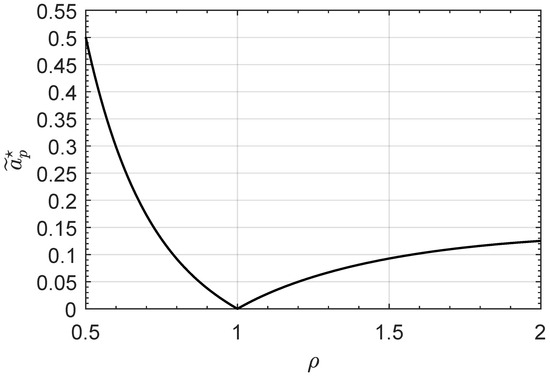
Figure 5. Reference value ${\tilde{a}}_p^{★}$ of the magnitude of dimensionless propulsive acceleration as a function of the mission parameter $\rho$.

Table 1. Value of the dimensionless reference propulsive acceleration magnitude ${\tilde{a}}_p^{★}$ and the dimensionless flight time ${\widetilde{\Delta t}}_H$ as a function of the design parameter $\rho \in [0.5,2]$, with $\rho \ne 1$.

$\mathit{\rho }$	${\tilde{\mathit{a}}}_{\mathit{p}}^{★}$	${\widetilde{\Delta \mathit{t}}}_{\mathit{H}}$
0.5000	0.5006	2.0405
0.5500	0.3867	2.1434
0.6000	0.2981	2.2479
0.6500	0.2284	2.3541
0.7000	0.1728	2.4619
0.7500	0.1282	2.5714
0.8000	0.0920	2.6823
0.8500	0.0624	2.7949
0.9000	0.0379	2.9089
0.9500	0.0174	3.0245
0.9900	0.0033	3.1181
1.0100	0.0032	3.1652
1.0500	0.0150	3.2601
1.1000	0.0280	3.3801
1.1500	0.0395	3.5016
1.2000	0.0497	3.6244
1.2500	0.0589	3.7487
1.3000	0.0671	3.8743
1.3500	0.0745	4.0014
1.4000	0.0812	4.1297
1.4500	0.0872	4.2595
1.5000	0.0927	4.3905
1.5500	0.0976	4.5229
1.6000	0.1020	4.6566
1.6500	0.1061	4.7915
1.7000	0.1097	4.9278
1.7500	0.1130	5.0653
1.8000	0.1160	5.2041
1.8500	0.1187	5.3441
1.9000	0.1211	5.4853
1.9500	0.1232	5.6278
2.0000	0.1252	5.7715

The function ${\tilde{a}}_p^{★}={\tilde{a}}_p^{★}\left(\rho \right)$, which is numerically obtained through the solution of a number of optimization problems, can be used to express the inequality constraint given by Equation (6) in a simple manner. To this end, we introduce an auxiliary dimensionless term $k_a\in [0,1]$ defined as

$$k_a={\displaystyle \frac{{\tilde{a}}_p}{{\tilde{a}}_p^{★}}}$$

(24)

so that, for an assigned mission scenario (i.e., for an assigned value of $\rho$ and, then, of ${\tilde{a}}_p^{★}$), the propulsive acceleration magnitude depends only in the auxiliary parameter $k_a$. In particular, the limit case of $k_a=0$ refers to the CHT (i.e., only the high-thrust propulsion system is installed onboard the spacecraft), while the case of $k_a=1$ refers to the scenario where the spacecraft uses only the continuous-thrust system to complete the transfer without impulsive maneuvers. In the generic scenario in which $k_a\ne \{0,1\}$, the value of the total velocity change due to the two impulsive maneuvers is calculated using the optimization approach described in the Section 3.3.

3.3. Minimization of the Total Velocity Change of Impulsive Maneuvers

Consider the scenario where both $k_a\in (0,1)$ and the dimensionless design parameter $\rho$ are assigned. Therefore, the AHT requires a total velocity change $\Delta v_A$, due to the two tangential impulsive maneuvers, different from zero in order to complete the transfer with the given flight time $\Delta t_H$ and the assigned sweep angle $\Delta {\theta }_H=\pi$ rad. In this case, the variation of the thrust angle $\alpha$ during the transfer can be selected in order to minimize the value of $\Delta v_A$. In dimensionless terms, this corresponds to maximize the performance index $J_v$ defined as

$$J_v\triangleq -{\widetilde{\Delta v}}_{i_A}^2-{\widetilde{\Delta v}}_{f_A}^2\equiv -{\left({\tilde{v}}_{{\theta }_i}-1\right)}^2-{\left({\tilde{v}}_{{\theta }_f}-\sqrt{1/\rho }\right)}^2$$

(25)

The maximization of the performance index given by the previous equation is obtained by using, again, the calculus of variations. In this context, the adjoint variables are $\{{\lambda }_r,{\lambda }_{\theta },{\lambda }_{v_r},{\lambda }_{v_{\theta }}\}$ and many of the results obtained in the previous section can be still used. In fact, also in this case, the Hamiltonian function is given by Equation (17), the Euler–Lagrange relations are given by Equations (18)–(21), and the optimal control law is still given by Equation (23). The main difference lies in the transversality condition which, in this case, provides the following two relations

$${\lambda }_{v_{\theta }}\left({\tilde{t}}_0\right)=2{\tilde{v}}_{{\theta }_i}-2,{\lambda }_{v_{\theta }}\left({\tilde{t}}_f\right)=-2{\tilde{v}}_{{\theta }_f}+{\displaystyle \frac{2}{\sqrt{\rho }}}$$

(26)

Therefore, the set of four dimensionless unknowns $\{{\lambda }_r\left({\tilde{t}}_0\right),{\lambda }_{\theta }\left({\tilde{t}}_0\right),{\lambda }_{v_r}\left({\tilde{t}}_0\right),{\tilde{v}}_{{\theta }_i}\}$ is determined so as to satisfy the four terminal constraints given by the first three relations in Equation (12) and by the last relation in Equation (26). Once the two-point boundary value problem is solved, the total velocity change ${\widetilde{\Delta v}}_A$ related to the two impulsive maneuvers in an AHT is an output of the numerical procedure. In this sense, the value of ${\widetilde{\Delta v}}_A$ is a function of two dimensionless terms, that is, the mission design parameter $\rho$ which defines the geometry of the transfer and $k_a$ which indicates the performance of the continuous-thrust propulsion system. The results of the numerical procedure are illustrated in the next Section 4.

4. Results of Numerical Simulations

The optimal control problem described in the previous section has been solved as a function of $k_a\in [0,1]$ and $\rho \in [0.5,2]$, considering an equally spaced set of 21 values for $k_a$ and 19 values for $\rho$. As a result, a total of $21\times 19=399$ optimization problems were solved to numerically obtain the functions ${\widetilde{\Delta v}}_{i_A}={\widetilde{\Delta v}}_{i_A}(k_a,\rho )$, ${\widetilde{\Delta v}}_{f_A}={\widetilde{\Delta v}}_{f_A}(k_a,\rho )$ and ${\widetilde{\Delta v}}_A={\widetilde{\Delta v}}_A(k_a,\rho )$, which, respectively, give the optimal value of the first, second, and total impulsive velocity change in an AHT.

The filled contour plots of the two functions ${\widetilde{\Delta v}}_{i_A}$ and ${\widetilde{\Delta v}}_{f_A}$ are reported in Figure 6, while Figure 7 shows the minimum value of the total (dimensionless) velocity change required by an AHT. As expected, Figure 7 clearly indicates that the use of the continuous-thrust propulsion system allows the total velocity change induced by tangential impulsive maneuvers to be reduced at will, up to zero in the limit case of $k_a\to 1$. This aspect also emerges from Figure 8, which instead shows the ratio between the total velocity change obtained in an AHT and that reached in a CHT. For example, when $\rho =0.5$ a value of $k_a\simeq 0.425$ allows the total velocity change $\Delta v_A$ to reach $50\%$ of the value obtained in a CHT.

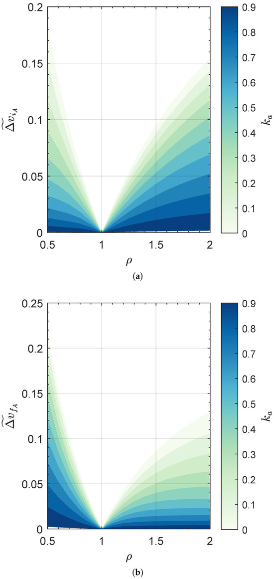
Figure 6. Optimal value of the dimensionless velocity change in the first and second tangential impulsive maneuver as a function of $k_a$ and $\rho \in [0.5,2]$, with $\rho \ne 1$. (a) First impulsive maneuver; (b) second impulsive maneuver.

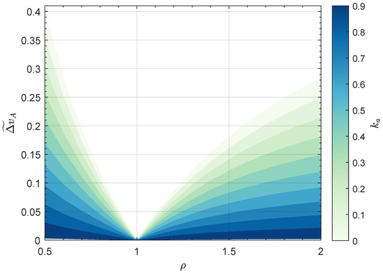
Figure 7. Minimum value of the total (dimensionless) velocity change in an AHT as a function of $k_a$ and $\rho \in [0.5,2]$, with $\rho \ne 1$.

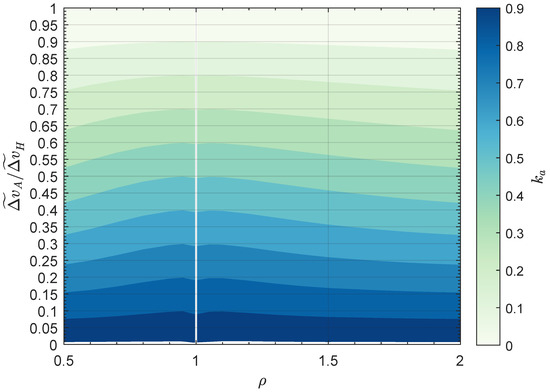
Figure 8. Ratio between the minimum value of the total velocity change ${\widetilde{\Delta v}}_A$ in an AHT and the value ${\widetilde{\Delta v}}_H$ analytically obtained in a CHT, as a function of $k_a$ and $\rho \ne 1$.

The numerical results discussed in this section and summarized in Figure 6, Figure 7 and Figure 8 are general, in the sense that they do not depend on the particular primary body around which the transfer occurs (i.e., on the value of the gravitational parameter $\mu$) or on the specific value of the radius of the initial circular orbit $r_i$, but only on the ratio $\rho$ between the two orbital radii $r_f$ and $r_i$. A specific application of the mathematical model discussed in the previous section is instead reported in the next section, which presents some typical mission scenarios.

5. Case Studies and Possible Mission Scenarios

This section shows a possible application of an AHT in: (1) a heliocentric transfer, i.e., a mission scenario in which the primary body is the Sun so that the gravitational parameter used in the numerical simulations takes the value $\mu$ = 13,271,2439,935.5 km³/s²; (2) a geocentric case in which the primary body is the Earth, whose gravitational parameter is $\mu$ = 398,600 km³/s² and the (mean) reference radius is equal to 6378 km. In particular, the heliocentric case is used to model both a simplified Earth–Venus and Earth–Mars transfer, while the geocentric case refers to a circular orbit raising of 100 km, with a parking circular orbit consistent with a typical LEO whose altitude is about 300 km.

5.1. Heliocentric Mission Scenarios

Consider the case in which the spacecraft initially covers a heliocentric circular orbit of radius $r_i=1 \text{AU}$, so that the value of the gravitational acceleration along the initial (circular) orbit is $\mu /r_i^2\simeq 5.93$ mm/s². Assume a target, coplanar, circular orbit with radius $r_f=0.723 \text{AU}$ (or $r_f=1.524 \text{AU}$), so that the dimensionless design parameter is $\rho =0.723$ (or $\rho =1.524$). Note that this scenario approximates an interplanetary transfer from Earth to Venus (or Mars) in the case in which both the orbital eccentricity and the orbital inclination over the Ecliptic of the target planet is neglected. The results in terms of the total velocity change $\Delta v_A$ of the two tangential impulsive maneuvers as a function of $a_p$ are summarized in Figure 9, while Table 2 reports some transfer parameters as the flight time and the velocity changes in a CHT. The variation with $a_p$ of the velocity changes $\Delta v_{i_A}$ and $\Delta v_{f_A}$ of the two impulsive maneuvers, in an AHT, are finally reported in Figure 10. Note that all velocity changes tend to zero as $a_p\to a_p^{★}$, as expected; see Table 2 for the value of $a_p^{★}$.

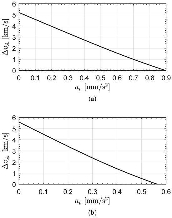
Figure 9. Total velocity change in an AHT as a function of $a_p$. (a) Case of an Earth–Venus transfer; (b) Case of an Earth–Mars transfer.

Table 2. Mission parameters in the two heliocentric transfers, Earth–Venus and Earth–Mars, in which $r_i=1\mathrm{AU}$.

Scenario	${\mathit{r}}_{\mathit{f}}$	$\Delta {\mathit{t}}_{\mathit{H}}$	$\Delta {\mathit{v}}_{{\mathit{i}}_{\mathit{H}}}$	$\Delta {\mathit{v}}_{{\mathit{f}}_{\mathit{H}}}$	$\Delta {\mathit{v}}_{\mathit{H}}$	${\mathit{a}}_{\mathit{p}}^{★}$
Earth–Venus	$0.723\mathrm{AU}$	$146\mathrm{days}$	$2.499\mathrm{km}/\mathrm{s}$	$2.711\mathrm{km}/\mathrm{s}$	$5.21\mathrm{km}/\mathrm{s}$	$0.8962\mathrm{mm}/{\mathrm{s}}^2$
Earth–Mars	$1.524\mathrm{AU}$	$258.9\mathrm{days}$	$2.946\mathrm{km}/\mathrm{s}$	$2.65\mathrm{km}/\mathrm{s}$	$5.596\mathrm{km}/\mathrm{s}$	$0.5639\mathrm{mm}/{\mathrm{s}}^2$

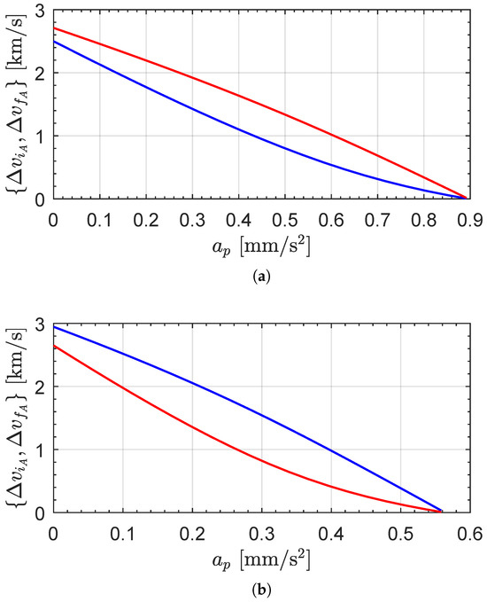
Figure 10. Velocity changes $\Delta v_{i_A}$ and $\Delta v_{f_A}$ of the two tangential impulsive maneuvers in an AHT as a function of $a_p$. Blue line → first maneuver ($\Delta v_{i_A}$); red line → second maneuver ($\Delta v_{f_A}$). (a) Case of an Earth–Venus transfer; (b) Case of an Earth–Mars transfer.

The spacecraft transfer trajectory in the two interplanetary mission scenarios considered in this section, in the case where the dimensionless ratio is $k_a=0.99$ as defined in Equation (24), is shown in Figure 11. In particular, according to Equation (24), that value of $k_a$ indicates that the magnitude $a_p$ of the propulsive acceleration vector induced by the continuous-thrust propulsion system is $99\%$ of the reference value $a_p^{★}$, which refers to a transfer achieved using only the steerable thrust vector. Using the data from Table 2, the value of $a_p$ employed to obtain the trajectories plotted in Figure 11 is, therefore, 0.558 mm/s² for the Mars case, and 0.887 mm/s² for the Venus case. In other words, the spacecraft transfer trajectories for the AHT case, which are plotted in Figure 11 with a green dashed line, are substantially consistent with a scenario where the entire circle-to-circle orbit transfer is achieved without the support of the high-thrust propulsion system providing the two impulsive (tangential) velocity changes. In that case, indeed, the value of the total velocity change $\Delta v_A$ is essentially zero, according to the plots in Figure 9. Figure 11 clearly indicates that the spacecraft transfer trajectory in this rather limit case of $a_p\simeq a_p^{★}$ is very close to the Hohmann’s semi-ellipse, indicated by a black line in the figure. This is because the optimization problem is solved by fixing both the initial position of the spacecraft and the swept angle during the transfer. Furthermore, the spacecraft transfer trajectories computed with different values of $k_a$ give lines that substantially overlap with the trajectories drawn in Figure 9.

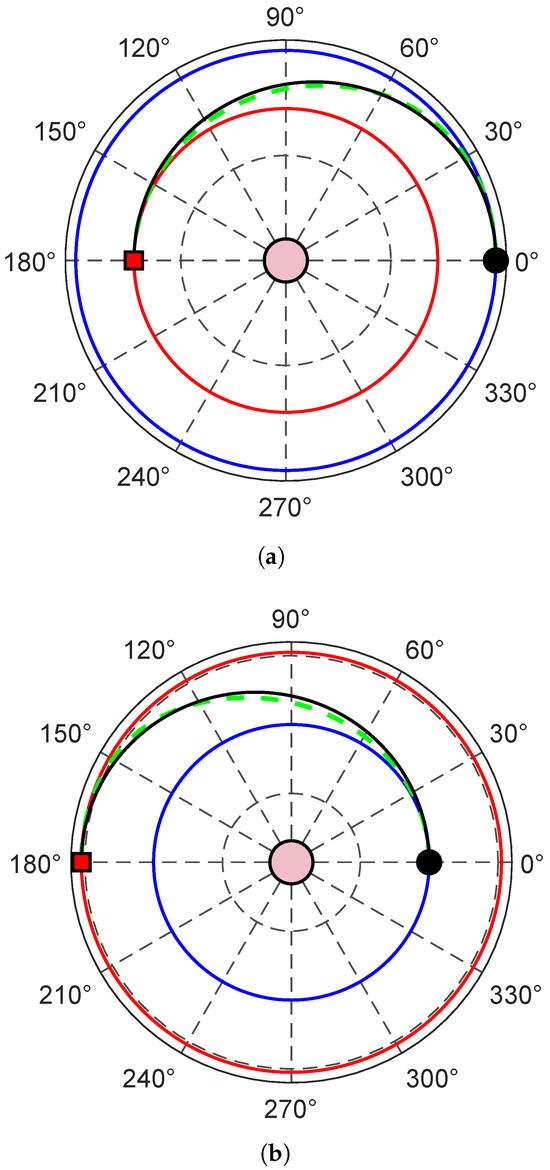
Figure 11. Spacecraft transfer trajectory when $k_a=0.99$ and the propulsive acceleration magnitude is $99\%$ of the reference value $a_p^{★}$ indicated in Table 2. Blue line → Earth’s orbit; red line → target planet orbit; black line → spacecraft trajectory in a CHT case; green dashed line → spacecraft trajectory in an AHT case; black dot → starting point; red square → arrival point; pink circle → the Sun. (a) Case of an Earth–Venus transfer; (b) Case of an Earth–Mars transfer.

The results of the numerical simulations can also be used to estimate the total velocity change of the circle-to-circle transfer, that is, the sum of the (minimum) velocity change $\Delta v_A$ due to the two tangential impulsive maneuvers and the velocity change $\Delta v_e$ related to the use of the continuous-thrust propulsion system. Bearing in mind that the continuous-thrust propulsion system is always switched on, the magnitude of the propulsive acceleration is a constant of motion, and the flight time is equal to $\Delta t_H=\Delta t_H\left(\rho \right)$, the value of $\Delta v_e$ can be simply obtained as

$$\Delta v_e=a_p\Delta t_H$$

(27)

which is, therefore, a function of $a_p$ and $\rho$. The sum of $\Delta v_A$ and $\Delta v_e$ for the two heliocentric mission scenarios is drawn, as a function of $a_p$, in Figure 12, which shows that the minimum value (as expected) is reached when the transfer is performed by using the two tangential impulsive maneuvers only. However, this result does not necessarily mean that the propellant consumption is lower in the scenario where only the high-thrust propulsion system is used, since the mass consumption value depends on the relative size of the specific impulse of the two thrusters. A study in this direction is left to the next future work.

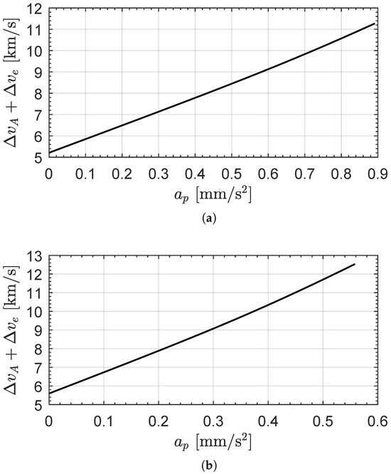
Figure 12. Sum of $\Delta v_A$ and $\Delta v_e$ as a function of $a_p$. (a) Case of an Earth–Venus transfer; (b) Case of an Earth–Mars transfer.

5.2. Geocentric Scenario

The second mission scenario is a geocentric transfer from a circular orbit of altitude equal to 300 km and a circular, coplanar, orbit of altitude 400 km. Accordingly, in this simple orbit raising the dimensionless ratio between the two orbital radii is given by $\rho =(6378\text{km}+400\text{km})/(6378\text{km}+300\text{km})=1.015$, while the Earth’s gravitational acceleration along the circular parking orbit is $\mu /r_i^2\simeq 8.94$ m/s² being $r_i=6678$ km. Table 3 summarizes some parameters of this specific orbit transfer.

Table 3. Mission parameters in the geocentric orbit raising.

${\mathit{r}}_{\mathit{i}}$	${\mathit{r}}_{\mathit{f}}$	$\Delta {\mathit{t}}_{\mathit{H}}$	$\Delta {\mathit{v}}_{{\mathit{i}}_{\mathit{H}}}$	$\Delta {\mathit{v}}_{{\mathit{f}}_{\mathit{H}}}$	$\Delta {\mathit{v}}_{\mathit{H}}$	${\mathit{a}}_{\mathit{p}}^{★}$
$6678\mathrm{km}$	$6778\mathrm{km}$	$45.76\min$	$28.65\mathrm{m}/\mathrm{s}$	$28.55\mathrm{m}/\mathrm{s}$	$57.2\mathrm{m}/\mathrm{s}$	$41.95\mathrm{mm}/{\mathrm{s}}^2$

The results of the numerical simulations, in terms of velocity changes as a function of $a_p$, are reported in Figure 13, where it can be observed that the plots of $\Delta v_{i_A}=\Delta v_{i_A}\left(a_p\right)$ and $\Delta v_{f_A}=\Delta v_{f_A}\left(a_p\right)$ are substantially overlapped due to the small value of the spacecraft altitude change during the transfer. Clearly, the one just presented is only a possible application to a geocentric case of the mathematical model proposed in this paper and of the general numerical results obtained through numerical simulations.

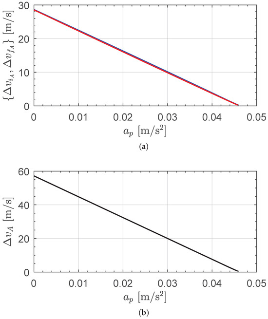
Figure 13. Velocity changes $\Delta v_{i_A}$, $\Delta v_{f_A}$, and $\Delta v_A$ as a function of $a_p$ in a geocentric orbit raising. (a) Velocity change of each impulsive maneuver: blue line → first impulsive maneuver ($\Delta v_{i_A}$); red line → second impulsive maneuver ($\Delta v_{f_A}$). (b) Total velocity change ($\Delta v_A$).

6. Conclusions

The use of an advanced propulsion system, which combines the characteristics of a chemical engine capable of generating a high thrust-to-weight ratio and the characteristics of a low-thrust engine capable of providing continuous and freely steerable propulsive acceleration vector in an orbital reference frame, is potentially capable of generating spacecraft trajectories capable of carrying out some typical space missions with very interesting performances.

In this case, one of the most interesting mission scenarios that can be analyzed in the context of a potential use of the advanced propulsion system such as the one described above, is the one concerning the transfer between two circular and coplanar orbits through a transfer trajectory that involves the use of two purely tangential impulses (performed at the initial and final instants of the transfer), and both the time-of-flight and the angular position change that recall the classic Hohmann maneuver. This sort of augmented Hohmann transfer has been studied in this paper considering, in the role of the continuous-thrust propulsion system that is employed in the time interval between the two tangential impulsive maneuvers, the general case of a spacecraft thruster able to provide a propulsive acceleration of constant magnitude during the whole flight. The use of this rather generalized type of continuous-thrust propulsion system concept allows to extend the results obtained in recent literature regarding the use of a photonic solar sail in supporting an augmented Hohmann transfer.

In this context, the paper shows to the reader the mathematical model capable of determining the optimal transfer performances in terms of the minimum value of the total velocity change required to complete the circular orbit transfer. Such optimal performances, which allows the designer to rapidly obtain the minimum value of the velocity change of the two tangential impulsive maneuvers, are calculated as a function of the propulsive acceleration magnitude of the continuous-thrust propulsion system and of the geometry of the Keplerian orbits involved in the transfer mission, that is, the ratio between the two radii of the parking and target circular orbit. In particular, as a by-product of the more general study of the transfer with combined employment of continuous-thrust and impulsive (tangential) endpoints maneuvers, this paper determines also the global minimum value of the constant propulsive acceleration which can be used during the transfer. This minimum value, which is necessary to correctly initialize the optimal control problem that allows the study of the augmented Hohmann transfer, is obtained by transferring the spacecraft with continuous-thrust to the target circular orbit, constraining both the time of flight and the final angular position to the typical values of the classical Hohmann transfer. The availability of such a minimum value of propulsive acceleration as a function of the characteristics of the two circular orbits is certainly an added value to the content of this article, since this result can also be used in the scenario in which the spacecraft is equipped exclusively with the continuous-thrust propulsion system.

The results of the numerical simulations indicated that an augmented Hohmann transfer can be performed by reducing the velocity change of the two impulsive maneuvers to zero, provided that the continuous-thrust propulsion system is capable of providing an adequate (constant) propulsive acceleration during the flight. In the case in which the velocity change related to the use of the continuous-thrust propulsion system is also considered, the mathematical model presented in this work allows for an accurate and fast estimate of the total value as a function of the geometric characteristics of the transfer. As expected, if the total velocity change is considered, the minimum value is reached when only the two impulsive maneuvers at the extremes of the transfer trajectory are used and, consequently, the limit case of zero (continuous) propulsive acceleration during the flight is assumed. However, this result could be misleading in light of the actual propellant consumption required by the transfer. In fact, typically continuous-thrust propulsion systems have a specific impulse value that is an order of magnitude higher than that typical of chemical systems that allow the impulsive maneuvers to be schematized within the transfer trajectory. In this sense, the reduction of the velocity change linked to the two impulsive maneuvers could lead to a mass saving much higher than that linked to the increase in propellant due to the operation of the continuous-thrust propulsion system. However, this aspect must be studied carefully, since it is also necessary to consider the increase in launch mass related to the presence of the additional propulsion system. Furthermore, in some mission scenarios, such as heliocentric ones, the velocity change relative to the first impulsive maneuver could be provided by the last stage of the launch system and, in this sense, its impact on the spacecraft mass distribution could be separated from the problem.

In any case, the mission scenario studied in this work can be considered as a first and simple approximation of the most common case, where the continuous-thrust propulsion system coincides with a typical solar electric thruster, in which the thrust magnitude is varied during the propellant consumption to maintain a constant value of the propulsive acceleration. The use of an effective propulsion system, and therefore, the knowledge of the real specific impulse of both the chemical engine that provides the two impulsive maneuvers and the electric engine that provides the continuous-thrust, will allow to study the augmented Hohmann maneuver also from the point of view of the total propellant mass required to achieve the circle-to-circle orbit transfer. This interesting aspect of the problem, whose foundations are exactly laid by the mathematical model presented in this paper, is currently under study and will represent the direct extension of the results discussed here.

References

- Gobetz, F.W.; Doll, J.R. A survey of impulsive trajectories. AIAA J. 1969, 7, 801–834. [Google Scholar] [CrossRef]
- Bate, R.R.; Mueller, D.D.; White, J.E. Fundamentals of Astrodynamics; Dover Publications: New York, NY, USA, 1971; Chapter 3; pp. 163–166. ISBN 0-486-60061-0. [Google Scholar]
- Prussing, J.E.; Conway, B.A. Orbital Mechanics; Oxford University Press: New York, NY, USA, 1993; Chapter 6; pp. 103–108. [Google Scholar]
- Junkins, J.L.; Schaub, H. Analytical Mechanics of Space Systems, 2nd ed.; American Institute of Aeronautics and Astronautics, Inc.: Reston, VA, USA, 2009; Chapter 13; pp. 621–626. ISBN 978-1-60086-721-7. [Google Scholar] [CrossRef]
- Curtis, H.D. Orbital Mechanics for Engineering Students; Butterworth-Heinemann: Oxford, UK, 2020; Chapter 6; pp. 289–295. ISBN 978-0-08-102133-0. [Google Scholar] [CrossRef]
- Hohmann, W. Die Erreichbarkeit der Himmelskörper; Verlag Von R. Oldenbourg: Berlin, Germany, 1925. [Google Scholar]
- Betts, J.T. Survey of Numerical Methods for Trajectory Optimization. J. Guid. Control. Dyn. 1998, 21, 193–207. [Google Scholar] [CrossRef]
- Bell, D.J. Optimal Space Trajectories—A Review of Published Work. Aeronaut. J. 1968, 72, 141–146. [Google Scholar] [CrossRef]
- Walsh, M.T.; Peck, M.A. Survey of Methods for Calculating Impulsive ΔV-Minimizing Orbit Transfer Maneuvers. In Proceedings of the AIAA Scitech 2020 Forum, Orlando, FL, USA, 6–10 January 2020. [Google Scholar] [CrossRef]
- Lawden, D.F. Optimal Trajectories for Space Navigation; Butterworths & Co.: London, UK, 1963; Chapter 6; pp. 106–110. [Google Scholar]
- Palmore, J. An Elementary Proof Of the Optimality of Hohmann Transfers. J. Guid. Control. Dyn. 1984, 7, 629–630. [Google Scholar] [CrossRef]
- Prussing, J.E. Simple proof of the global optimality of the Hohmann transfer. J. Guid. Control. Dyn. 1992, 15, 1037–1038. [Google Scholar] [CrossRef]
- Pontani, M. Simple Method to Determine Globally Optimal Orbital Transfers. J. Guid. Control. Dyn. 2009, 32, 899–914. [Google Scholar] [CrossRef]
- Quarta, A.A.; Mengali, G.; Niccolai, L.; Bianchi, C. Solar Sail Augmented Hohmann Transfer. IEEE Trans. Aerosp. Electron. Syst. 2023, 59, 2065–2071. [Google Scholar] [CrossRef]
- Fu, B.; Sperber, E.; Eke, F. Solar sail technology—A state of the art review. Prog. Aerosp. Sci. 2016, 86, 1–19. [Google Scholar] [CrossRef]
- Gong, S.; Macdonald, M. Review on solar sail technology. Astrodynamics 2019, 3, 93–125. [Google Scholar] [CrossRef]
- Spencer, D.A.; Johnson, L.; Long, A.C. Solar sailing technology challenges. Aerosp. Sci. Technol. 2019, 93, 105276. [Google Scholar] [CrossRef]
- Zhao, P.; Wu, C.; Li, Y. Design and application of solar sailing: A review on key technologies. Chin. J. Aeronaut. 2023, 36, 125–144. [Google Scholar] [CrossRef]
- McInnes, C.R. Solar radiation pressure. In Solar Sailing: Technology, Dynamics and Mission Applications; Springer-Praxis Series in Space Science and Technology; Springer: Berlin, Germany, 1999; pp. 46–54. [Google Scholar] [CrossRef]
- McInnes, C.R. Solar sail orbital dynamics. In Solar Sailing: Technology, Dynamics and Mission Applications; Springer-Praxis Series in Space Science and Technology; Springer: Berlin, Germany, 1999; pp. 119–120. [Google Scholar] [CrossRef]
- Levchenko, I.; Goebel, D.; Pedrini, D.; Albertoni, R.; Baranov, O.; Kronhaus, I.; Lev, D.; Walker, M.L.; Xu, S.; Bazaka, K. Recent innovations to advance space electric propulsion technologies. Prog. Aerosp. Sci. 2025, 152, 100900. [Google Scholar] [CrossRef]
- Casanova-Álvarez, M.; Navarro-Medina, F.; Tommasini, D. Feasibility study of a Solar Electric Propulsion mission to Mars. Acta Astronaut. 2024, 216, 129–142. [Google Scholar] [CrossRef]
- Tsien, H.S. Take-Off from Satellite Orbit. J. Am. Rocket. Soc. 1953, 23, 233–236. [Google Scholar] [CrossRef]
- Boltz, F.W. Orbital Motion Under Continuous Radial Thrust. J. Guid. Control. Dyn. 1991, 14, 667–670. [Google Scholar] [CrossRef]
- Boltz, F.W. Orbital Motion Under Continuous Tangential Thrust. J. Guid. Control. Dyn. 1992, 15, 1503–1507. [Google Scholar] [CrossRef]
- Quarta, A.A. Continuous-Thrust Circular Orbit Phasing Optimization of Deep Space CubeSats. Appl. Sci. 2024, 14, 7059. [Google Scholar] [CrossRef]
- Baig, S.; McInnes, C.R. Artificial Three-Body Equilibria for Hybrid Low-Thrust Propulsion. J. Guid. Control. Dyn. 2008, 31, 1644–1655. [Google Scholar] [CrossRef]
- Mengali, G.; Quarta, A.A. Tradeoff performance of hybrid low-thrust propulsion system. J. Spacecr. Rocket. 2007, 44, 1263–1270. [Google Scholar] [CrossRef]
- Burke, L.M.; Oleson, S.R.; Zoloty, Z.C.; Smith, D.; Havens, M. Combined 1-MW Solar Electric and Chemical Propulsion for Crewed Mars Missions. In Proceedings of the ASCEND 2023, Las Vegas, NV, USA, 23–25 October 2023. [Google Scholar] [CrossRef]
- Chai, P.; Merrill, R.G.; Qu, M.; Shen, H. Integrated Optimization of Mars Hybrid Solar-Electric/Chemical Propulsion Trajectories. In Proceedings of the 2018 AIAA SPACE and Astronautics Forum and Exposition, Orlando, FL, USA, 17–19 September 2018. [Google Scholar] [CrossRef]
- Chai, P.; Qu, M.; Saputra, B. Human Mars Mission In-Space Transportation Sensitivity for Nuclear Electric/Chemical Hybrid Propulsion. In Proceedings of the AIAA Propulsion and Energy 2021 Forum, Virtual event, 9–11 August 2021. [Google Scholar] [CrossRef]
- Chobotov, V.A. (Ed.) Orbital Maneuvers. In Orbital Mechanics; AIAA Education Series: Reston, VA, USA, 2002; Chapter 5; pp. 94–96. ISBN 978-1563471797. [Google Scholar] [CrossRef]
- Chobotov, V.A. (Ed.) Complications to Impulsive Maneuvers. In Orbital Mechanics; AIAA Education Series: Reston, VA, USA, 2002; Chapter 6; pp. 117–119. ISBN 978-1563471797. [Google Scholar] [CrossRef]
- Bryson, A.E.; Ho, Y.C. Applied Optimal Control; Hemisphere Publishing Corporation: New York, NY, USA, 1975; Chapter 2; pp. 71–89. ISBN 0-891-16228-3. [Google Scholar]
- Stengel, R.F. Optimal Control and Estimation; Dover Books on Mathematics; Dover Publications, inc.: New York, NY, USA, 1994; pp. 222–254. ISBN 978-0486682006. [Google Scholar]
- Prussing, J.E. Spacecraft Trajectory Optimization; Cambridge University Press: Cambridge, UK, 2010; Chapter 2; pp. 16–36. ISBN 978-1107653825. [Google Scholar] [CrossRef]
- Quarta, A.A. Initial costate approximation for rapid orbit raising with very low propulsive acceleration. Appl. Sci. 2024, 14, 1124. [Google Scholar] [CrossRef]
- Ross, I.M. A Primer on Pontryagin’s Principle in Optimal Control; Collegiate Publishers: San Francisco, CA, USA, 2015; Chapter 2; pp. 127–129. [Google Scholar]
- Quarta, A.A. Preliminary Trajectory Analysis of CubeSats with Electric Thrusters in Nodal Flyby Missions for Asteroid Exploration. Remote Sens. 2025, 17, 513. [Google Scholar] [CrossRef]
Disclaimer/Publisher’s Note: The statements, opinions and data contained in all publications are solely those of the individual author(s) and contributor(s) and not of MDPI and/or the editor(s). MDPI and/or the editor(s) disclaim responsibility for any injury to people or property resulting from any ideas, methods, instructions or products referred to in the content. |
© 2025 by the author. Licensee MDPI, Basel, Switzerland. This article is an open access article distributed under the terms and conditions of the Creative Commons Attribution (CC BY) license (https://creativecommons.org/licenses/by/4.0/).