Design and Analysis of a Launcher Flight Control System Based on Incremental Nonlinear Dynamic Inversion ^†

Abstract

This paper investigates the application of Incremental Nonlinear Dynamic Inversion (INDI) for launch vehicle flight control, addressing the limited exploration of nonlinear control architectures and their potential benefits in the context of the current “New Space” era. In this context, this study aims to bridge the gap between the launcher’s traditional linear control practice and nonlinear methods, focusing on INDI, which offers the potential to enhance limits of performance while reducing mission preparation (“missionisation”) efforts. INDI control commands incremental inputs by exploiting feedback acceleration estimates in a feedback-linearised plant in order to reduce model dependency, making it easier to design and resulting in a robust closed loop as compared to nonlinear dynamic inversion. The objective of this paper is therefore to demonstrate INDI’s implementation in a representative industrial launch ascent scenario, evaluate its strengths and limitations relative to industry standards, and promote its adoption within the launcher Guidance, Navigation, and Control (GNC) community. Comparative simulations with traditional scheduled PD controllers, with and without angular acceleration feedback, are highlighted together with several trade-offs. Furthermore, this paper presents a new and practical INDI stability analysis method as applied in the context of aerospace attitude control, as well as an augmentation of the design with an outer control loop for active load relief. Results indicate that while INDI exhibits increased sensitivity to sensor noise and actuator delays as compared to the linear controllers, its advantages in robustness and performance are significant. Notably, INDI’s ability to handle nonlinearities without extensive tuning and gain-scheduling surpasses the capabilities of the traditional linear control counterparts. These results highlight the potential of INDI as a more robust and efficient alternative to state-of-practice launcher control design methodologies.

1. Introduction

1.1. Background and Motivation

The space industry has undergone a significant transformation in recent years, characterised by the emergence of the “New Space” era. This era is marked by disruptive changes in business models, manufacturing technologies, and agile development practices within launch vehicle companies, all aimed at minimising production and operating costs in an increasingly competitive market. Despite this focus on innovation, the potential benefits of advancements in control theory, such as increasing performance limits and streamlining mission preparation (or “missionisation”) efforts, have received limited attention.

Moreover, government-led developments of recent launchers such as Ares I and VEGA still adhere to the same design approach of the Saturn V, i.e., linear control [1]. This approach relies on single-channel tuning and ad hoc gain-scheduling followed by extensive validation and verification (V&V) processes, all of which are time-consuming and resource-intensive.

In contrast to the approach presented above, the past few years have seen a growing interest in the application of artificial intelligence and machine learning methods for launcher GNC, but the industrial use of such data-driven/model-free methods remains limited by well-known issues related to training and certification of the algorithms on the full flight envelope of intended operation. In that sense, there is a clear gap between these strategies and the current state of practice, in which other techniques could bring relevant improvements; this is the case for nonlinear control algorithms, especially those based on Nonlinear Dynamic Inversion (NDI). On the one hand, agile practices of New Space companies provide the ideal opportunity to explore the benefits of this type of design approach. On the other hand, a successful adoption of nonlinear launcher control will likely facilitate the augmentation with and transition to data-driven methods in the future. This is therefore our motivation and aim for this paper, to start bridging the gap between these two approaches while presenting a potential alternative based on incremental nonlinear control.

1.2. Related Work

In this paper, we briefly introduce and focus on (Incremental) Nonlinear Dynamic Inversion (NDI), which is a control design method based on feedback linearisation [2,3]; it basically consists of a nonlinear (state feedback) transformation that linearises the nominal system dynamics and a linear part that imposes the desired closed-loop dynamics. NDI is a very well-known and applied (nonlinear) control technique in the aerospace field, especially in aeronautics for various flight control applications [4,5,6,7,8]. Successful implementation of NDI requires a match between the onboard model and the system model and accurate knowledge of all nonlinearities, which is often not the case in reality; this results in poor robustness properties because they rely on exact availability of the system dynamics. This highlights the need for robustness in these methodologies, as the inner loop of the control system is critical and can be compromised by model and sensor uncertainties, potentially affecting stability and performance. In this regard, alternative methods involving robustness and improvements of the method for NDI-based flight control applications were considered, among many others, in [9,10,11,12,13].

A successful technique that became popular in recent years for aerospace applications is Incremental Nonlinear Dynamics Inversion (INDI). The concept using incremental nonlinear control was first developed in the late 1990s and was initially focused on the “implicit” dynamic inversion for DI-based flight control. The works of Smith, Bacon, and others laid the foundation for these developments [6,11], for which the term “incremental” is now more commonly used to describe this methodology as it better reflects the nature of these control laws [14,15,16]. Those early studies further developed the incremental approach, and since then, it has been further elaborated theoretically and successfully applied in various high-performance systems including fault-tolerant control of aircraft subjected to sensor and actuator faults [17,18], in practice for quadrotors using adaptive control [19,20], in real flight tests of small (unmanned) and business jet (Cessna Citation II, PH-LAB) aircraft [21,22,23]; it has also been used in studies in spacecraft attitude control [24,25,26], and it is planned to be flight-tested in the upcoming “Reusability Flight Experiment (ReFEx)” by DLR [27,28,29,30]. However, its applicability to launch vehicles has not been fully investigated yet but only considered in [31,32,33,34] and more recently in [35]. These related works have demonstrated INDI’s performance and robustness against aerodynamic model uncertainties and disturbance rejection for several aerospace vehicles; hence, the potential benefits of INDI are quite relevant for reusable launchers which have much tighter dynamical couplings between online-generated trajectory and attitude control during descent flight. Moreover, due to the nonlinear nature of INDI, it has proven difficult to attain analytical proof of stability, which has been derived in [36].

With this paper, which is an extended and improved version of [37], we aim to further close this gap towards the application of INDI for launchers, with special focus on the ascent of a TVC-controlled launcher, and also to present a new, practical approach for stability analysis of such INDI control laws applied for attitude control. Furthermore, the extension from [37] in this work considers an outer loop for load relief control to handle the uncontrolled drift dynamics that arise when performing attitude control only.

1.3. Objectives and Outline

It is therefore the objective of this paper to showcase the implementation of INDI on a representative application scenario; to highlight its strengths and limitations in the face of the industrial state of practice; and to raise awareness of the INDI method among the launcher GNC community. To achieve this, this paper provides a concise description of the NDI and INDI approaches, followed by the detailed design and comparison of different control laws: linear, linear with angular acceleration feedback, and INDI-based. Furthermore, this paper also aims to address the (main) two well-known challenges associated with the practical implementation of INDI-based control:

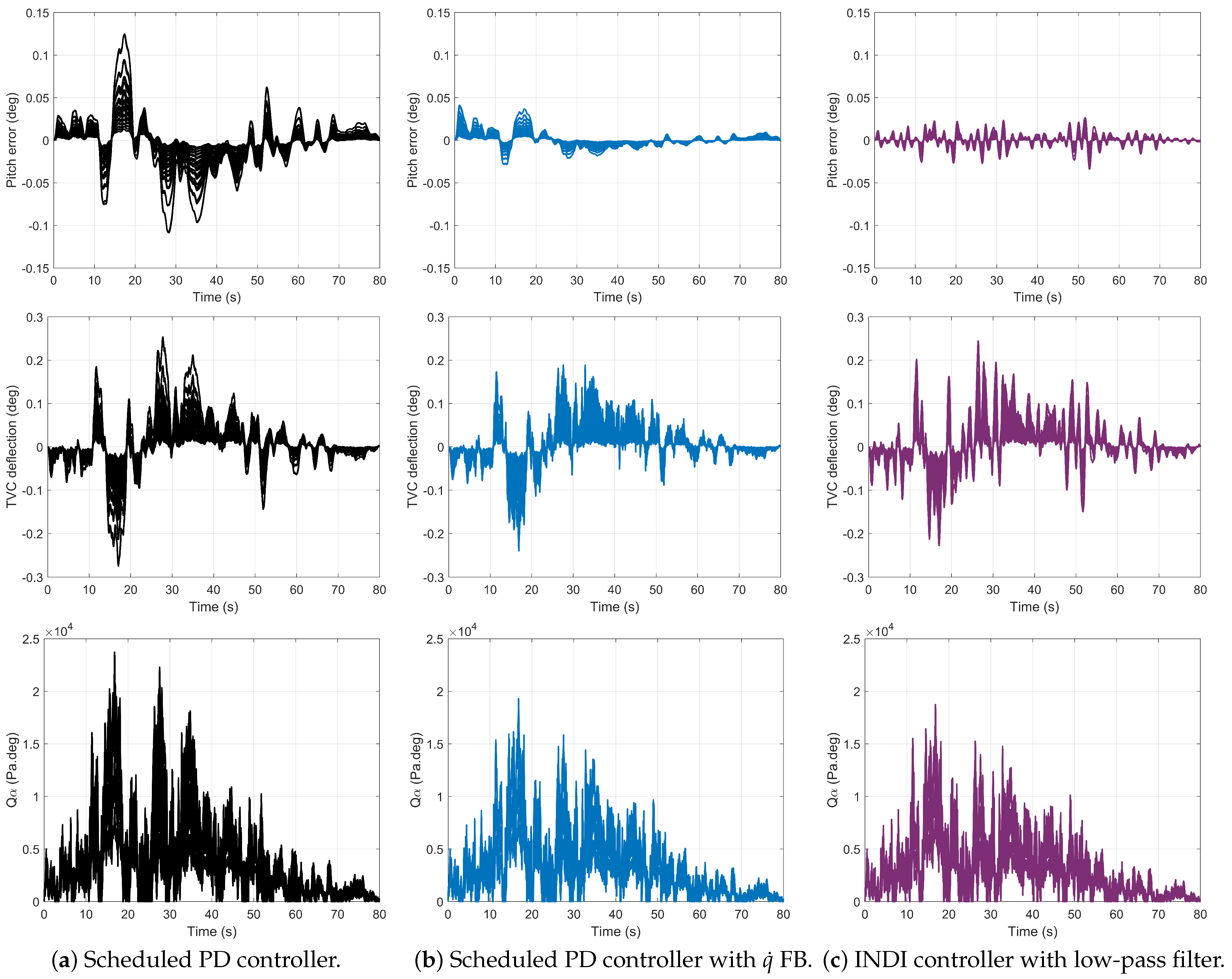
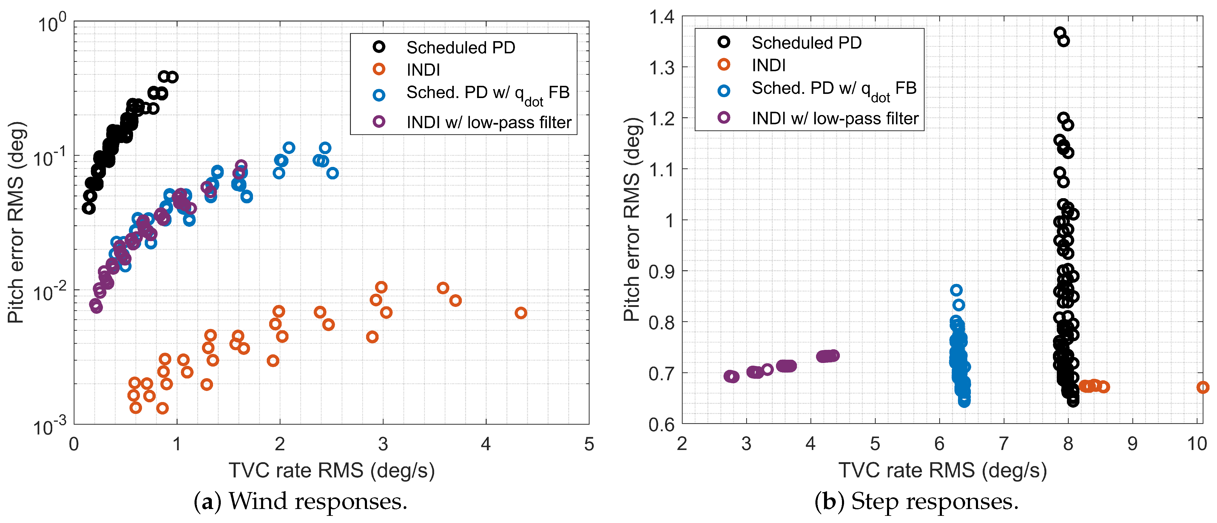
• Sensitivity to sensor noise and actuator delay. By relying on angular acceleration and control input measurements/estimates, INDI controllers are generally more sensitive to sensor noise and actuator delay than classical controllers. To assess the severity of this challenge, this paper shows a comprehensive nonlinear simulation campaign with wind disturbances and uncertainties, as well as different levels of sensor noise and actuator delay. These simulations serve as a basis to analyse the sensitivity to sensor noise and actuator delay in comparison to more classical approaches, and we showcase how to remediate or tackle these issues properly.
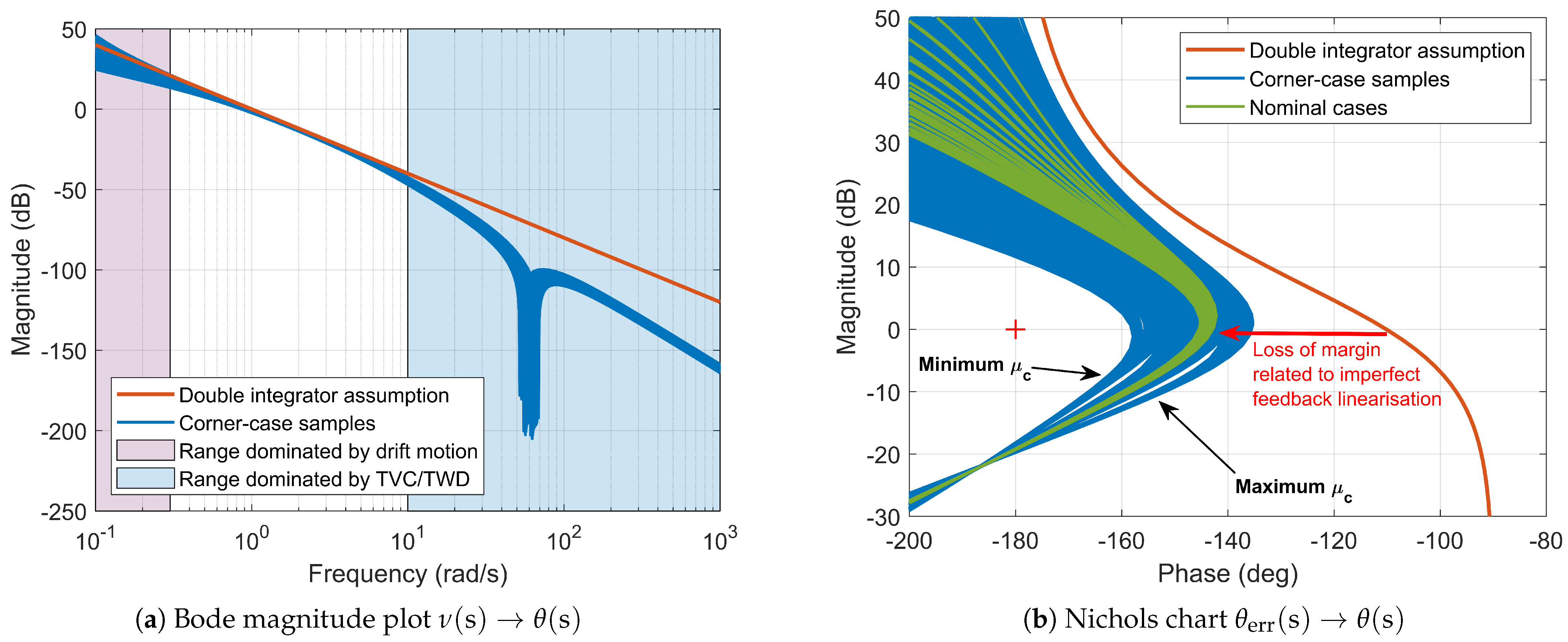
• Nonlinear stability analysis. The second challenge of INDI is that due to its nonlinear nature, attaining analytical proof of stability is not trivial [36]. For this second challenge, this paper proposes a simple yet insightful linearisation-based approach to evaluate stability degradation related to an inexact feedback linearisation and to deviations from the control tuning conditions. This method provides a new way to analyse and evaluate stability analysis of the nonlinear controller using linear control techniques; since INDI is designed from the theory of feedback linearisation, this approach is very intuitive in the sense that it provides a measure of degradation with respect to the feedback-linearised plant, and linear stability analysis can be performed.

Lastly, this paper also addresses improvements and extensions of [37] regarding load relief. This is necessary within this launch vehicle ascent context because of the “internal” dynamics that arises when performing (I)NDI for attitude control only; therefore, we address the following challenge:

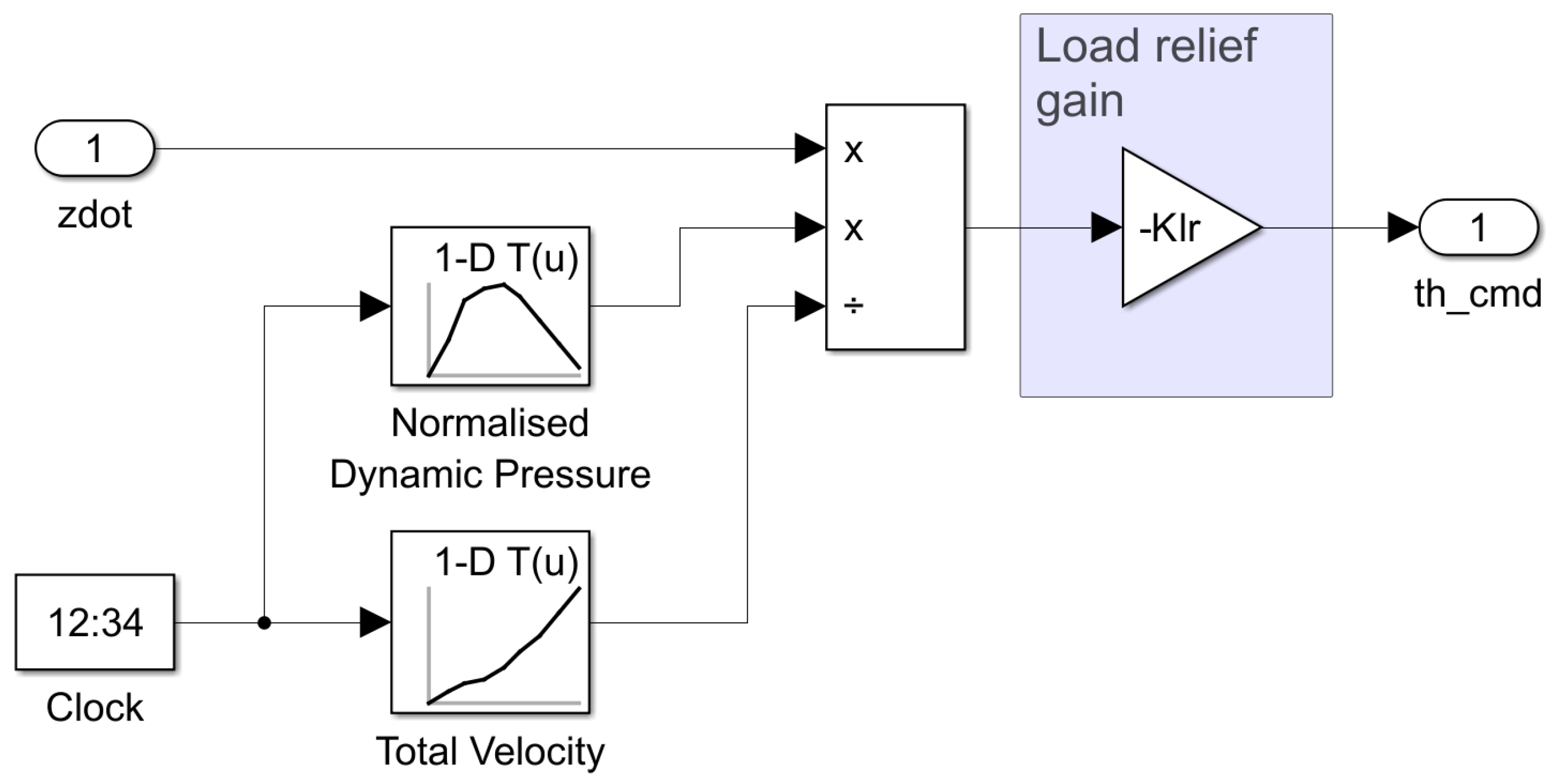
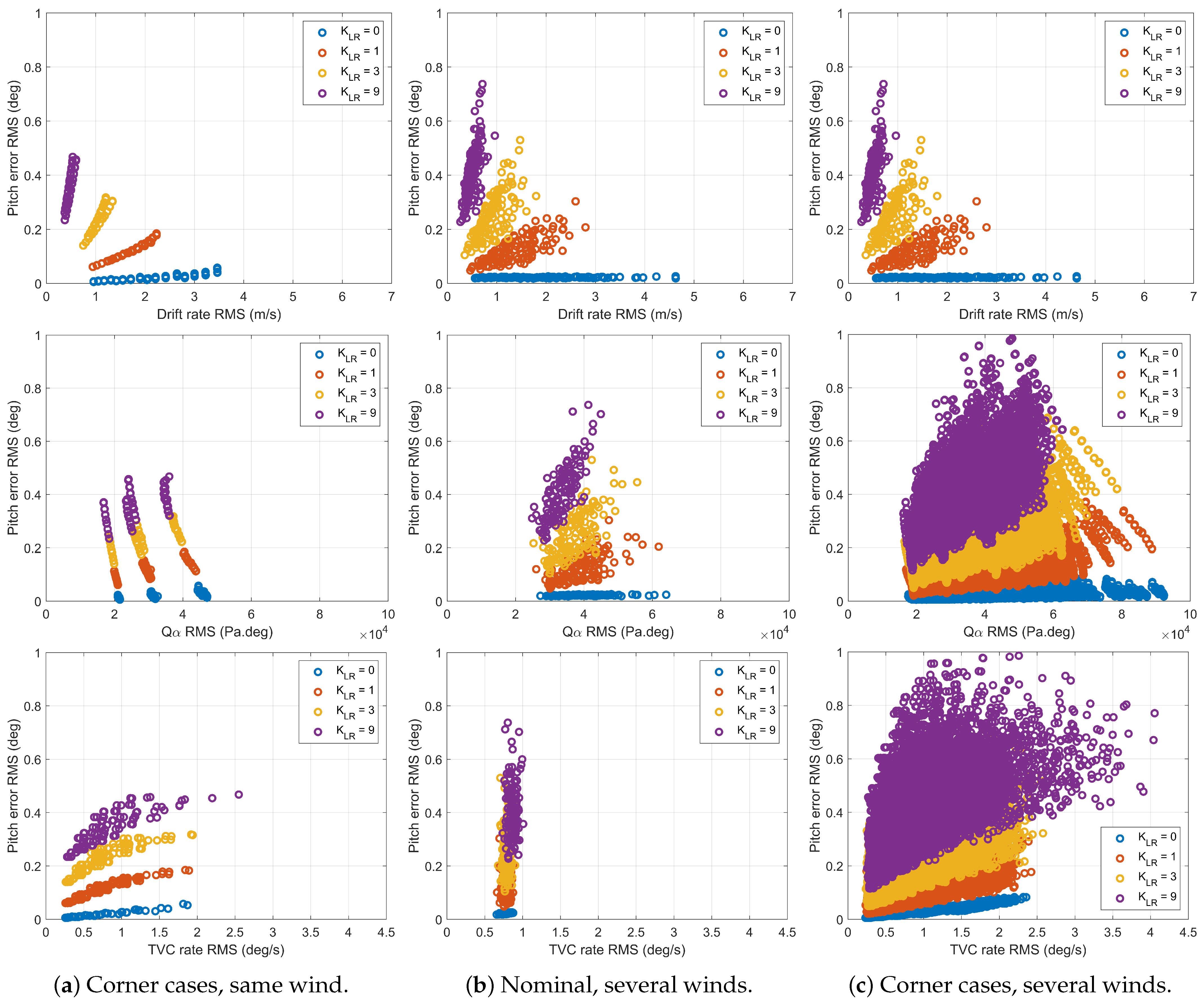
• Drift dynamics. We propose an extension to our launcher flight control system including an active load relief outer loop. Since the drift states can grow unbounded depending on the attitude control architecture, an outer loop providing the reference pitch angle for the inner-loop attitude and rate control can alleviate the drift and mitigate aerodynamic loads during ascent.

To demonstrate the benefits and challenges of the INDI approach, we showcase the method within an application scenario consisting of a launcher model during ascent flight while featuring attitude and lateral drift degrees of freedom, actuator dynamics, and moving-mass effects. All the controllers and filters are implemented at a sampling frequency that is compatible with current onboard capabilities (25 Hz).

The outline of this paper is as follows. A brief introduction to Nonlinear Dynamic Inversion (NDI) and Incremental NDI is presented in Section 2. Section 3 presents the launch flight dynamics modelling aspects and describes the simulator used for the attitude control design and testing. Launcher attitude control designs including angular acceleration feedback are presented in Section 4. Time-domain robust performance results and analysis of the obtained simulations comparing the controllers studied are presented in Section 5, while Section 6 presents the frequency-domain stability results and analysis. Section 7 presents an extension to flight control with active load relief, and finally, conclusions are presented in Section 8.

2. Basic Principles of (Incremental) Nonlinear Dynamic Inversion

2.1. Nonlinear Dynamic Inversion (NDI)

We consider a multiple-input and multiple-output (MIMO) system whose number of inputs are equal to the number of outputs without loss of generality, to avoid control allocation complexities. Let us also assume momentarily that the nonlinear system can be described affine in the inputs as

$$\dot{x}=f\left(x\right)+g\left(x\right)u$$

(1a)

$$y=h\left(x\right)$$

(1b)

where $x\in R^n$ is the state vector, $u\in R^m$ is the control input vector, and $y\in R^m$ is the system output vector, the functions $f\left(x\right)$ and $h\left(x\right)$ are assumed to be smooth vector fields on Rⁿ, and $g\left(x\right)\in R^{n\times m}$ is a matrix whose columns are also assumed as smooth vector fields $g_j$. For these systems, the vector of relative degree $\mathit{\rho }$ represents the number of differentiations of each output $y_i$, $i=1,\dots ,m$, that are needed for the input to appear [2,3]. Moreover, the vector of the relative degree of the continuous-time nonlinear system satisfies $\rho ={∥\rho ∥}_1\le n$, where $\rho$ is the total relative degree of the system. In this brief introduction to NDI, we consider y = x so that the relative degree of each output $y_i$ is one, and therefore the system is said to be full-state feedback-linearisable. Whenever the total relative degree is strictly less than the order of the system ($\rho <n$), the nonlinear system is then decomposed into an external (input–output) part and an internal (unobservable) part which is described by a new set of ($n-\rho$)-coordinates [26,36].

Nonlinear Dynamic Inversion (NDI) is a technique that aims to eliminate the nonlinearities present in a given nonlinear system, resulting in closed-loop dynamics that can be expressed in a linear form. To achieve this, the nonlinear system is inverted into a linear structure using state feedback, making it possible to apply conventional linear controllers. However, NDI has a significant disadvantage in that it relies on the fundamental assumption that the system model is known exactly, making it vulnerable to uncertainties. Additionally, NDI assumes that the system state is fully and accurately known, which can be challenging to achieve in practice. NDI involves applying the following input transformation [2,3]:

$$u_{\mathrm{cmd}}=g^{-1}\left(x\right)\left(v-f\left(x\right)\right)$$

(2)

which cancels all nonlinearities in a closed loop, and the simple linear input–output relationship or “single-integrator” form $\dot{y}=v$ between the new virtual control input v and the output y is obtained. In the case that the relative degree of each output $y_i$ is 2, the relationship would be a double integrator $\stackrel{\mathrm{..}}{y}=v$, and so on. In addition to being linear, an interesting feature of this relationship is that it is also decoupled, meaning that the input ${\nu }_i$ only affects the output $y_i$; this property makes (2) a decoupling control law. By utilising appropriate control techniques (e.g., linear, robust), the single-integrator form can be rendered exponentially stable. The single integrator can be made exponentially stable through the use of

$$\begin{array}{c}\hfill v={\dot{y}}_{\mathrm{des}}\end{array}$$

(3)

where, for instance, ${\dot{y}}_{\mathrm{des}}={\dot{y}}_{\mathrm{cmd}}+K_{P}e$ defines the desired dynamics for the output vector or control variables. Here, ${\dot{y}}_{\mathrm{cmd}}$ is a feedforward term, while $e=y_{\mathrm{cmd}}-y$ represents the error vector, and $y_{\mathrm{cmd}}$ denotes the (smooth) desired output vector which is (in this case, since the relative degree is one) at least once-differentiable. The gain matrix $K_P\in R^{m\times m}$ is used to ensure that the polynomials given by $s+K_{P_i}$ for $i=1,\dots ,m$ become Hurwitz. The diagonal elements $K_{P_i}$ of $K_P$ are then selected accordingly. As a result of using (3), the desired error dynamics ${\dot{e}}_i+K_{P_i}{e}_i=0$ become exponentially stable and decoupled, leading to $e_i\left(t\right)\to 0$ for $i=1,\dots ,m$. Here, ${\dot{y}}_{\mathrm{des}}$ can be designed in any other way as long as the closed-loop system remains stable while guaranteeing desired performance requirements.

2.2. Incremental Nonlinear Dynamic Inversion (INDI)

Incremental Nonlinear Dynamic Inversion (INDI) consists of the application of NDI to a system expressed in an incremental form [15,16,36]. To obtain a system in incremental form, first we introduce a sufficiently small time delay $\lambda$ and define the following deviation variables ${\dot{x}}_0:=\dot{x}(t-\lambda )$, $x_0:=x(t-\lambda )$, and $u_0:=u(t-\lambda )$; these are the $\lambda$-time-delayed signals of the current state derivative $\dot{x}\left(t\right)$, state $x\left(t\right)$, and control $u\left(t\right)$, respectively [25]. Moreover, we denote $\mathrm{\Delta }\dot{x}:=\dot{x}-{\stackrel{.}{x}}_0$, $\mathrm{\Delta }x:=x-x_0$, and $\mathrm{\Delta }u:=u-u_0$ as the incremental state derivative, the incremental state, and the so-called incremental control input, respectively. Subsequently, we consider a first-order Taylor series expansion of $\dot{x}$ not in the geometric sense but with respect to the newly introduced time delay $\lambda$ as [15,16,25,36]

$$\begin{array}{cc}\hfill \dot{x}=& {\dot{x}}_0+{\displaystyle \frac{\partial }{\partial x}}\left[f\left(x\right)+g\left(x\right)u\right]{|}_{\begin{array}{c}x=x_0\\ u=u_0\end{array}}\mathrm{\Delta }x+g\left(x_0\right)\mathrm{\Delta }u+H.O.T\hfill \\ & ={\dot{x}}_0+g\left(x_0\right)\mathrm{\Delta }u+N(x,\lambda )\hfill \end{array}$$

(4)

with ${\dot{x}}_0=f\left(x_0\right)+g\left(x_0\right)u_0$ and

$$\begin{array}{cc}\hfill N(x,\lambda )& ={\displaystyle \frac{\partial }{\partial x}}\left[f\left(x\right)+g\left(x\right)u\right]{|}_{\begin{array}{c}x=x_0\\ u=u_0\end{array}}\mathrm{\Delta }x+H.O.T\hfill \end{array}$$

(5)

which represents a residual containing the Jacobian linearisation of the onboard model and the higher-order terms ($H.O.T$) of the series expansion. Notice that the model-based control effectiveness $g\left(x_0\right)$ is sampled at the previous incremental time. This means an approximate linearisation about the λ—delayed signals is performed incrementally and not with respect to a particular equilibrium or operational point of interest.

Furthermore, it is assumed that during a sufficiently small time increment $\lambda$ (i.e., for a sufficiently high control frequency), the input u can change significantly faster than the state x [15,16,25,36]. This implies that there is a reasonable frequency separation between the dynamics of the vehicle and of the actuators, which is generally the case for aerospace systems. Under this assumption, the following approximation holds:

$$\mathrm{\Delta }x=x-x_0\cong 0, \mathrm{even} \mathrm{if} \mathrm{\Delta }u=u-u_0\ne 0$$

(6)

which leads to

$$\begin{array}{cc}\hfill \dot{x}\cong & {\dot{x}}_0+g\left(x_0\right)\mathrm{\Delta }u+\underset{\cong 0}{\underbrace{N(x,\lambda )}}\Rightarrow \mathrm{\Delta }\dot{x}\cong g\left(x_0\right)\mathrm{\Delta }u\hfill \end{array}$$

(7)

This assumption, corroborated by the fact that the perturbation term $N(x,\lambda )$ satisfies [36]:

$$\underset{\lambda \to 0}{\lim }{∥N(x,\lambda )∥}_2\to 0,\forall x$$

(8)

implies that the nonlinear system dynamics in its incremental form is approximated at each time-step by the model-based control effectiveness $g\left(x_0\right)$. Finally, applying NDI to the system based on the approximation (7) results in a relation between the incremental control input and the output of the system:

$$u=u_0+{u\left(x_0\right)}^{-1}(v-{\dot{x}}_0)$$

(9)

It shall be noted that the availability of ${\dot{x}}_0$ is required, and that the incremental input $u_0$ is obtained from the output of the actuators or estimated from an actuator dynamical model; recall it has been assumed that a commanded control is achieved sufficiently fast with regard to the actuator dynamics. The total control command along with the obtained linearising control $u_0=u(t-\lambda )$ can be rewritten as

$$u\left(t\right)=u(t-\lambda )+{g\left(x(t-\lambda )\right)}^{-1}[v-\dot{x}(t-\lambda )]$$

(10)

This improves the robustness of the closed-loop system as compared with conventional NDI since dependency on the accurate knowledge of the plant dynamics is reduced; more specifically, the dependency on accurate knowledge of the dynamic model in $f\left(x\right)$ is largely decreased. Therefore, the INDI control law design is more dependent on accurate measurements or accurate estimates of ${\dot{x}}_0$, the state derivatives, and $u_0$, the incremental control input, respectively. INDI control is therefore model- and sensor-based because of the model-based control effectiveness $g\left(x_0\right)$ and the necessity to measure or sense the additional quantities of $u_0$ and ${\dot{x}}_0$.

3. Launcher Flight Dynamics and Control Synthesis Models

3.1. Flight Dynamics

The present study relies on a conventional single-axis launcher model in ascent flight featuring lateral drift (z) and pitch ($\theta$) dynamics, as schematised in Figure 1. These dynamics, representing the first and second time derivatives of z as { $\dot{z}=w$, $\ddot{z}=\dot{w}$ } together with the first and second time derivatives of $\theta$ as { $\dot{\theta }=q$, $\ddot{\theta }=\dot{q}$ }, are governed by the well-known nonlinear Newton–Euler equations:

$$\begin{array}{cc}\hfill m\dot{w}& =F_{\alpha }+F_{\mathrm{c}}+F_{\mathrm{n}}-mg\sin \theta \hfill \end{array}$$

(11a)

$$\begin{array}{cc}\hfill J\dot{q}& =M_{\alpha }+M_{\mathrm{c}}+M_{\mathrm{n}}\hfill \end{array}$$

(11b)

where m, J, and g are the launcher’s mass, lateral moment of inertia, and gravity acceleration, respectively; {$F_{\alpha }$, $M_{\alpha }$} are the normal aerodynamic forces and moments, respectively; {$F_{\mathrm{c}}$, $M_{\mathrm{c}}$} are the TVC-induced forces and moments, respectively; and {$F_{\mathrm{n}}$, $M_{\mathrm{n}}$} are the engine nozzle moving-mass effects, also known as tail-wags-dog (TWD).

The aerodynamic force consists of an axial component (A in Figure 1) and a normal component ($N_{\alpha }\alpha$), which varies linearly with the angle of attack $\alpha$. Only the latter is considered in this single-axis launcher model, and the induced force and moment are computed as

$$\begin{array}{cc}\hfill F_{\alpha }& =-N_{\alpha }\alpha =-S{C}_{N_{\alpha }}Q\alpha \hfill \end{array}$$

(12a)

$$\begin{array}{cc}\hfill M_{\alpha }& =-l_{\alpha }{F}_{\alpha }=l_{\alpha }S{C}_{N_{\alpha }}Q\alpha \hfill \end{array}$$

(12b)

where S, $C_{N_{\alpha }}$, and $l_{\alpha }$ are the reference aerodynamic area, lateral force gradient, and aerodynamic arm (distance between the launcher’s centres of pressure and gravity). $Q\alpha$ is the aerodynamic load indicator, defined as the product between aerodynamic pressure and angle of attack, which are, respectively, given by

$$\begin{array}{cc}\hfill Q& ={\displaystyle \frac{1}{2}}\rho V^2\hfill \end{array}$$

(13a)

$$\begin{array}{cc}\hfill \alpha & =\theta +arctan{\displaystyle \frac{w-l_{\alpha }q-v_{\mathrm{w}}}{V}}\hfill \end{array}$$

(13b)

where $\rho$ is the air density, V is the total airspeed, and $v_{\mathrm{w}}$ is the lateral wind turbulence speed. The term $l_{\alpha }q$ is often known as aerodynamic damping. The TVC-induced force and moment are computed as

$$\begin{array}{cc}\hfill F_{\mathrm{c}}& =-T\sin \beta \hfill \end{array}$$

(14a)

$$\begin{array}{cc}\hfill M_{\mathrm{c}}& =l_{\mathrm{c}}{F}_{\mathrm{c}}=-l_{\mathrm{c}}T\sin \beta \hfill \end{array}$$

(14b)

where T is the thrust magnitude, $l_{\mathrm{c}}$ is the TVC arm (distance between the launcher’s centre of gravity and nozzle’s pivot point), and $\beta$ is the TVC deflection angle. Finally, the nozzle TWD effects (dynamics) are computed as

$$\begin{array}{cc}\hfill F_n& =-m_n{l}_n\ddot{\beta }\hfill \end{array}$$

(15a)

$$\begin{array}{cc}\hfill M_n& =l_c{F}_n-J_n\ddot{\beta }=-(m_n{l}_n{l}_c+J_n)\ddot{\beta }\hfill \end{array}$$

(15b)

where $m_{\mathrm{n}}$ is the nozzle moving mass, $l_{\mathrm{n}}$ is the moving-mass arm (distance between the nozzle’s centre of gravity and pivot point), $\ddot{\beta }$ is the TVC deflection acceleration, and $J_{\mathrm{n}}$ is the nozzle moment of inertia with respect to the pivot point (not to the centre of gravity).

Most of the model’s parameters vary along the launcher’s trajectory (this dependence was not evidenced in the previous equations for the sake of readability) and are highly uncertain. These parameters were extracted as a function of time from the simulator presented in [38] for an 80 s trajectory. The uncertainty levels adopted in this study are summarised in

Table 1. Uncertainty level per type of parameter.

Type of Parameters	Variables	Uncertainty Level
Aerodynamics	$C_{N_{\alpha }}$, $l_{\alpha }$, $\rho$, V	20%
Mass/propulsion	m, J, $l_{\mathrm{c}}$, T	10%

and are assumed to remain constant throughout the flight.

Note that while mass/propulsion parameters have an explicit dependency on time, related to the way the propellant burns, aerodynamics parameters have an implicit dependency through intermediate quantities such as altitude and Mach number.

3.2. Actuator Dynamics

In addition to the launcher model described above, the present study considers the dynamical effects of TVC actuation and wind turbulence. Both effects are modelled as time-invariant transfer functions for the sake of simplicity without loss of generality. The TVC dynamics corresponds to a reduced second-order model of the system used in [39], which is given by

$$G_{\mathrm{TVC}}\left(\mathrm{s}\right)={\displaystyle \frac{67.8^2}{{\mathrm{s}}^2+90.9 \mathrm{s}+67.8^2}}$$

(16)

where s represents the Laplace variable. The wind turbulence speed $v_{\mathrm{w}}$ is modelled by colouring a white noise signal through a first-order Dryden filter [40] given by

$$G_{\mathrm{w}}\left(\mathrm{s}\right)={\displaystyle \frac{3.54}{\mathrm{s}+0.32}}$$

(17)

The launcher, TVC, and wind models were put together in a simulator that allows us to quickly analyse and compare several control systems, which is illustrated in Figure 2. In this figure, different simulation rates are highlighted using different colours: black for the continuous-time dynamics, red for GNC computations ($f_{\mathrm{GNC}}=25$ Hz, which is well representative of current onboard capabilities), and green for wind noise generation ($f_{\mathrm{w}}=20$ Hz in this case).

3.3. Nonlinear Model

In this section, we conveniently express the dynamics in state-space form. For that, consider the following coefficients [39]; first, relative to the rotational motion,

$$\begin{array}{cc}\hfill {\overline{\mu }}_{\alpha }& ={\displaystyle \frac{l_{\alpha }Q\mathrm{s}{C}_{N_{\alpha }}}{J}}={\displaystyle \frac{l_{\alpha }{N}_{\alpha }}{J}}\hfill \end{array}$$

(18a)

$$\begin{array}{cc}\hfill {\overline{\mu }}_c& ={\displaystyle \frac{l_{c}T}{J}}\hfill \end{array}$$

(18b)

$$\begin{array}{cc}\hfill {\overline{\mu }}_n& ={\displaystyle \frac{m_n{l}_n{l}_c+J_n}{J}}\hfill \end{array}$$

(18c)

and second, relative to the translational motion,

$$\begin{array}{cc}\hfill {\overline{n}}_{\alpha }& ={\displaystyle \frac{Q\mathrm{s}{C}_{N_{\alpha }}}{m}}={\displaystyle \frac{N_{\alpha }}{m}}\hfill \end{array}$$

(19a)

$$\begin{array}{cc}\hfill {\overline{n}}_c& ={\displaystyle \frac{T}{m}}\hfill \end{array}$$

(19b)

$$\begin{array}{cc}\hfill {\overline{n}}_n& ={\displaystyle \frac{m_n{l}_n}{m}}\hfill \end{array}$$

(19c)

Then, considering the state vector $x={\left[z,\dot{z},\theta ,\dot{\theta }\right]}^{\top }={\left[z,w,\theta ,q\right]}^{\top }$, the full nonlinear system dynamics results in

$${\mathsf{\Sigma }}_{nonlin}:\left\{\begin{array}{cc}\dot{z}\hfill & =w,\hfill \\ \ddot{z}\hfill & =\dot{w}={\overline{n}}_{\alpha }\alpha -{\overline{n}}_c\sin \beta -{\overline{n}}_n\ddot{\beta }-g\sin \theta ,\hfill \\ \dot{\theta }\hfill & =q,\hfill \\ \ddot{\theta }\hfill & =\dot{q}={\overline{\mu }}_{\alpha }\alpha -{\overline{\mu }}_c\sin \beta -{\overline{\mu }}_n\ddot{\beta }\hfill \end{array}\right.$$

(20)

3.4. Synthesis and Linear Models

For control design purposes, it is convenient to express the dynamics using an approximated synthesis model that fully captures the driving dynamics of Equations (11a) and (11b). To do so, the coefficients in Equations (18) and (19) are extracted from a reference (nominal) trajectory and are now denoted without the bars. Using the small angles approximation, we can consider the following dynamics as the synthesis model:

$${\mathsf{\Sigma }}_{\mathrm{s}yn}:\left\{\begin{array}{cc}\dot{z}\hfill & =w\hfill \\ \ddot{z}\hfill & =\dot{w}=n_{\alpha }\alpha -n_c\beta -n_n\ddot{\beta }-g\sin {\theta }_0\hfill \\ \dot{\theta }\hfill & =q\hfill \\ \ddot{\theta }\hfill & =\dot{q}={\mu }_{\alpha }\alpha -{\mu }_c\beta -{\mu }_n\ddot{\beta }\hfill \end{array}\right.$$

(21)

Considering the output vector $y={\left[w, \theta \right]}^{\top }={\left[w\left(\mathrm{s}\right), \theta \left(\mathrm{s}\right)\right]}^{\top }$, we obtain the following linear system dynamics in the Laplace domain:

$${\mathsf{\Sigma }}_{lin}:\left\{\begin{array}{c}\mathrm{s}w\left(\mathrm{s}\right)-n_{\alpha }\alpha \left(\mathrm{s}\right)+g\sin {\theta }_0=-(n_n{\mathrm{s}}^2+n_c)\beta \left(\mathrm{s}\right)\hfill \\ {\mathrm{s}}^2\theta \left(\mathrm{s}\right)-{\mu }_{\alpha }\alpha \left(\mathrm{s}\right)=-({\mu }_n{\mathrm{s}}^2+{\mu }_c)\beta \left(\mathrm{s}\right)\hfill \end{array}\right.$$

(22)

and using the linearised angle of attack,

$$\alpha =\theta +{\displaystyle \frac{w-l_{\alpha }q-v_{\mathrm{w}}}{V}} \Rightarrow \alpha \left(\mathrm{s}\right)=\left(1-l_{\alpha }{\displaystyle \frac{1}{V}}\mathrm{s}\right)\theta \left(\mathrm{s}\right)+{\displaystyle \frac{1}{V}}w\left(\mathrm{s}\right)-{\displaystyle \frac{1}{V}}{v}_{\mathrm{w}}\left(\mathrm{s}\right)$$

(23)

together with the model in Equation (22), we obtain the transfer functions $\beta \left(\mathrm{s}\right)\to \theta \left(\mathrm{s}\right)$ and $\beta \left(\mathrm{s}\right)\to w\left(\mathrm{s}\right)$, which correspond to the solutions of the system (without the wind input $v_{\mathrm{w}}\left(\mathrm{s}\right)$):

$$\left[\begin{array}{cc}{\mathrm{s}}^2+l_{\alpha }{\displaystyle \frac{{\mu }_{\alpha }}{V}}\mathrm{s}-{\mu }_{\alpha }& -{\displaystyle \frac{{\mu }_{\alpha }}{V}}\\ -l_{\alpha }{\displaystyle \frac{n_{\alpha }}{V}}\mathrm{s}+n_{\alpha }+g\sin {\theta }_0& \mathrm{s}+{\displaystyle \frac{n_{\alpha }}{V}}\end{array}\right]\left[\begin{array}{c}{\displaystyle \frac{\theta \left(\mathrm{s}\right)}{\beta \left(\mathrm{s}\right)}}\\ {\displaystyle \frac{w\left(\mathrm{s}\right)}{\beta \left(\mathrm{s}\right)}}\end{array}\right]=-\left[\begin{array}{c}{\mu }_{\mathrm{n}}{\mathrm{s}}^2+{\mu }_{\mathrm{c}}\\ n_{\mathrm{n}}{\mathrm{s}}^2+n_{\mathrm{c}}\end{array}\right]$$

(24)

Furthermore, as a first approximation for attitude control design purposes, drift and TWD dynamics can be neglected, and the transfer function $\beta \left(\mathrm{s}\right)\to \theta \left(\mathrm{s}\right)$ simplifies into

$${\displaystyle \frac{\theta \left(\mathrm{s}\right)}{\beta \left(\mathrm{s}\right)}}=-{\displaystyle \frac{{\mu }_{\mathrm{c}}}{{\mathrm{s}}^2+l_{\alpha }{\displaystyle \frac{{\mu }_{\alpha }}{V}}\mathrm{s}-{\mu }_{\alpha }}}$$

(25)

4. Attitude Control Design Using Angular Acceleration Feedback

This section describes and justifies the four attitude control systems developed in this study.

4.1. Scheduled PD Controller

The baseline controller for this study is a classic proportional-derivative (PD) controller designed for the linear system approximation in Equation (25); the PD controller is therefore considered with the following structure:

$$\beta \left(\mathrm{s}\right)=k_P\left({\theta }_{\mathrm{cmd}}\left(\mathrm{s}\right)-\theta \left(\mathrm{s}\right)\right)-k_{D}q\left(\mathrm{s}\right)=k_P{\theta }_{\mathrm{cmd}}\left(\mathrm{s}\right)-\left(k_P+\mathrm{s}{k}_D\right)\theta \left(\mathrm{s}\right)$$

(26)

Despite their simplicity, PD controllers represent the industrial state of practice for the vast majority of launch vehicles [1]. The gains $k_P$ and $k_D$ can be tuned using a multitude of methods. Here, they are selected based on pole placement of the closed-loop transfer function, which is obtained by substituting Equation (26) in (25):

$${\displaystyle \frac{\theta \left(\mathrm{s}\right)}{{\theta }_{\mathrm{cmd}}\left(\mathrm{s}\right)}}=-{\displaystyle \frac{{\mu }_{\mathrm{c}}{k}_P}{{\mathrm{s}}^2+\left(l_{\alpha }{\displaystyle \frac{{\mu }_{\alpha }}{V}}-{\mu }_{\mathrm{c}}{k}_D\right)\mathrm{s}-\left({\mu }_{\alpha }+{\mu }_{\mathrm{c}}{k}_P\right)}}$$

(27)

It is clear from this equation that $k_P$ and $k_D$ can be chosen to enforce the desired natural frequency ${\omega }_{\theta }$ and damping ratio $\zeta$ (here assumed constant throughout the flight for simplicity without loss of generality). It is also clear that this approach does not allow us to specify the steady-state gain (when $\mathrm{s}\to 0$) independently of the natural frequency as they both depend on $k_P$ only.

In order to handle the wide variation of the model’s parameters during the flight, the two gains need to be scheduled throughout the trajectory. To do so, they are pre-computed for a grid of $N=9$ points (spaced every 10 seconds along the trajectory) as

$$k_P\left[i\right]=-{\displaystyle \frac{1}{{\mu }_{\mathrm{c}}\left[i\right]}}\left({\mu }_{\alpha }\left[i\right]+{\omega }_{\theta }^2\right),k_D\left[i\right]={\displaystyle \frac{1}{{\mu }_{\mathrm{c}}\left[i\right]}}\left(l_{\alpha }\left[i\right]{\displaystyle \frac{{\mu }_{\alpha }\left[i\right]}{V\left[i\right]}}-2\zeta {\omega }_{\theta }\right),i=1,\dots ,N$$

(28)

and then linearly interpolated online during the simulation. The robustness of this approach can be increased by scheduling the controller with respect to online measurements/estimates of some of the model’s parameters. This is the underlying idea of LPV control [41], which is outside the scope of this paper.

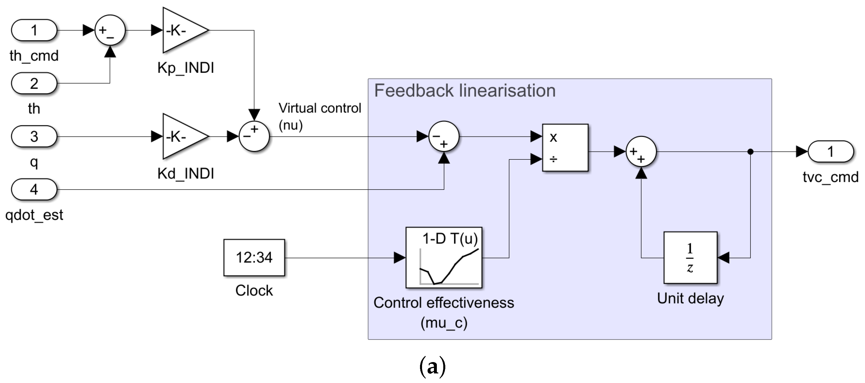
4.2. INDI Controller

In this section, an INDI-based control law is developed and applied to regulate the launcher’s attitude channel in Equation (21); therefore, we consider only the state $x_c={\left[\theta , \dot{\theta }\right]}^{\top }={\left[\theta , q\right]}^{\top }$, and ignoring the TWD effects, the dynamics are

$${\dot{x}}_c=f_c\left(x_c\right)+g_c\left(x_c\right)u=\left[\begin{array}{c}q\\ {\mu }_{\alpha }\alpha \end{array}\right]-\left[\begin{array}{c}0\\ {\mu }_c\end{array}\right]\beta$$

(29)

where $f_c\left(x_c\right)$ is the control-independent part of the model, $g_c\left(x_c\right)$ expresses the influence of the controls in the system, and $u=\beta$ is the control input, i.e., the TVC deflection. Considering the (scalar) output as $y=h\left(x\right)=\theta$, in order to apply the INDI technique, it has to be time-differentiated until an explicit dependency on the TVC deflection input appears:

$$\ddot{y}=\ddot{\theta }={\mu }_{\alpha }\alpha -{\mu }_c\beta$$

(30)

Then, while denoting $\nu$ as a virtual control input, the NDI control law for $\beta$ is obtained as

$${\beta }_{\mathrm{NDI}}=-{\displaystyle \frac{1}{{\mu }_c}}\left(\nu -{\mu }_{\alpha }\alpha \right)$$

(31)

Since ${\mu }_c$ is different from zero, the linear input–output relationship between $\ddot{\theta }$ and $\nu$ is obtained as a double integrator:

$$\nu =\dot{q}=\ddot{\theta }\Rightarrow {\displaystyle \frac{\theta \left(\mathrm{s}\right)}{\nu \left(\mathrm{s}\right)}}={\displaystyle \frac{1}{{\mathrm{s}}^2}}$$

(32)

Because of the high level of uncertainty affecting ${\mu }_{\alpha }$ and $\alpha$, it is convenient to employ the more robust INDI approach; for that, following the procedure of Section 2.2, the INDI control law results in a command signal sent to the TVC actuator given by

$$\beta ={\beta }_0-{\displaystyle \frac{1}{{\mu }_{\mathrm{c}}}}\left(\nu -{\dot{q}}_0\right)$$

(33)

where ${\beta }_0$ and ${\dot{q}}_0$ are measurements/estimates of the TVC command and angular acceleration at the current computation step, respectively. Because angular acceleration sensors are not common in launchers today, ${\dot{q}}_0$ is estimated by passing the angular rate q through a derivative filter of the form:

$$H_{\dot{q}}\left(\mathrm{s}\right)={\displaystyle \frac{\mathrm{s}{\omega }_{\dot{q}}}{\mathrm{s}+{\omega }_{\dot{q}}}}$$

(34)

where ${\omega }_{\dot{q}}$ represents the filter bandwidth.

Note that after the feedback linearisation of Equation (33), there are still some degrees of internal dynamics in the system related to the drift motion and TWD effect. However, the TWD dynamics are known to be stable, and the drift motion develops slowly and can be further handled by outer control loops (e.g., see Section 7). Denoting $e={\theta }_{\mathrm{cmd}}-\theta$, where ${\theta }_{\mathrm{cmd}}$ represents the (nonsmooth) commanded pitch angle (in this case, the only reference for the attitude motion), the double integrator can be therefore rendered exponentially stable with

$$\nu =k_D\dot{e}+k_{P}e$$

(35)

where $k_D$ and $k_P$ are constants chosen so that the polynomial ${\mathrm{s}}^2+k_D\mathrm{s}+k_P$ is Hurwitz. This results in the exponentially stable and decoupled error dynamics $\ddot{e}+k_D\dot{e}+k_{P}e=0$, which implies that $e\left(t\right)\to 0$ as $t\to \infty$. Using the virtual control and the linearised system of Equation (32), an outer PD control law is able to enforce the desired closed-loop response as follows:

$$\nu \left(\mathrm{s}\right)=k_P\left({\theta }_{\mathrm{cmd}}\left(\mathrm{s}\right)-\theta \left(\mathrm{s}\right)\right)-k_{D}q\left(\mathrm{s}\right)\Rightarrow {\displaystyle \frac{\theta \left(\mathrm{s}\right)}{{\theta }_{\mathrm{cmd}}\left(\mathrm{s}\right)}}={\displaystyle \frac{k_P}{{\mathrm{s}}^2+k_D\mathrm{s}+k_P}}$$

(36)

with the control gains:

$$k_P={\omega }_{\theta }^2,k_D=2\zeta {\omega }_{\theta }$$

(37)

Note that in contrast with the PD controller of Section 4.1, $k_P$ and $k_D$ do not need to be scheduled as they depend on ${\omega }_{\theta }$ and $\zeta$ only, but a pre-computed grid of ${\mu }_{\mathrm{c}}\left[i\right]$ is still required to perform the feedback linearisation. This is highlighted in the blue area of Figure 3a, which illustrates the implementation of the INDI controller in the simulator. Alternatively, ${\mu }_{\mathrm{c}}$ could be estimated based on online measurements. As also shown in Figure 3a, the feedback linearisation loop includes a unit delay to ensure physical causality of the signals.

4.3. Scheduled PD Controller with $\dot{q}$ Feedback

As explained in Section 2.2, the INDI controller of Equation (33) relies on $\dot{q}$ information to reduce the impact of the launcher’s model on the achievable control performance. For a fair comparison of controllers, it is then pertinent to consider a linear controller where $\dot{q}$ feedback is also employed. In this case, the control law takes the form

$$\beta \left(\mathrm{s}\right)=k_P\left({\theta }_{\mathrm{cmd}}\left(\mathrm{s}\right)-\theta \left(\mathrm{s}\right)\right)-k_{D}q\left(\mathrm{s}\right)-k_A\dot{q}\left(\mathrm{s}\right)$$

(38)

where $k_A$ is the acceleration feedback gain. Similar to Section 4.1, the three gains can be tuned via pole placement of the closed-loop transfer function, which is obtained by substituting Equation (38) in (25):

$${\displaystyle \frac{\theta \left(\mathrm{s}\right)}{{\theta }_{\mathrm{cmd}}\left(\mathrm{s}\right)}}=-{\displaystyle \frac{k_P}{1-{\mu }_{\mathrm{c}}{k}_A}}{\displaystyle \frac{{\mu }_{\mathrm{c}}}{{\mathrm{s}}^2+{\displaystyle \frac{l_{\alpha }\frac{{\mu }_{\alpha }}{V}-{\mu }_{\mathrm{c}}{k}_D}{1-{\mu }_{\mathrm{c}}{k}_A}}\mathrm{s}-{\displaystyle \frac{{\mu }_{\alpha }+{\mu }_{\mathrm{c}}{k}_P}{1-{\mu }_{\mathrm{c}}{k}_A}}}}$$

(39)

In contrast with the pure PD controller, the $\dot{q}$ feedback allows us to minimise tracking errors because the desired steady-state gain $G_0$ is specified independently of ${\omega }_{\theta }$ through the proportional gain as follows:

$$k_P\left[i\right]={\displaystyle \frac{{\mu }_{\alpha }\left[i\right]}{{\mu }_{\mathrm{c}}\left[i\right]}}{\displaystyle \frac{G_0}{1-G_0}},i=1,\cdots ,N$$

(40)

which is scheduled along a grid of $N=9$ points along the launcher’s trajectory. The other two gains are then derived as a function of ${\omega }_{\theta }$ and $\zeta$ as

$$k_A\left[i\right]={\displaystyle \frac{1}{{\mu }_{\mathrm{c}}\left[i\right]}}\left(1+{\displaystyle \frac{{\mu }_{\alpha }\left[i\right]+{\mu }_{\mathrm{c}}\left[i\right]k_P\left[i\right]}{{\omega }_{\theta }^2}}\right),k_D\left[i\right]={\displaystyle \frac{1}{{\mu }_{\mathrm{c}}\left[i\right]}}\left(l_{\alpha }\left[i\right]{\displaystyle \frac{{\mu }_{\alpha }\left[i\right]}{V\left[i\right]}}-2\zeta {\omega }_{\theta }\left(1-{\mu }_{\mathrm{c}}\left[i\right]k_A\left[i\right]\right)\right)$$

(41)

For the estimation of $\dot{q}$ in Equation (38), the same approach of Section 4.2, i.e., passing the angular rate q through the first-order derivative filter of Equation (34), was followed. In practice, it was verified that the performance of this controller is fairly sensitive to the filter bandwidth ${\omega }_{\dot{q}}$. This impact is illustrated in Figure 4, which shows root-mean-square (RMS) values of pitch error (${\theta }_{\mathrm{err}}={\theta }_{\mathrm{cmd}}-\theta$) vs. TVC rate ($\dot{\beta }$) for a step command in ${\theta }_{\mathrm{cmd}}$ using different controllers and nominal conditions.

The blue line in Figure 4 shows results using the scheduled PD controller with $\dot{q}$ feedback (FB) and varying values of the derivative filter bandwidth ${\omega }_{\dot{q}}$. Based on the results, the selection of ${\omega }_{\dot{q}}$ provides a key (and intuitive) tuning trade-off: increasing the bandwidth leads to smaller errors at the expense of more demanding TVC actuation, and vice versa. A more favourable trade-off would likely be achieved by using a higher-order-derivative filter, which is outside the scope of this paper.

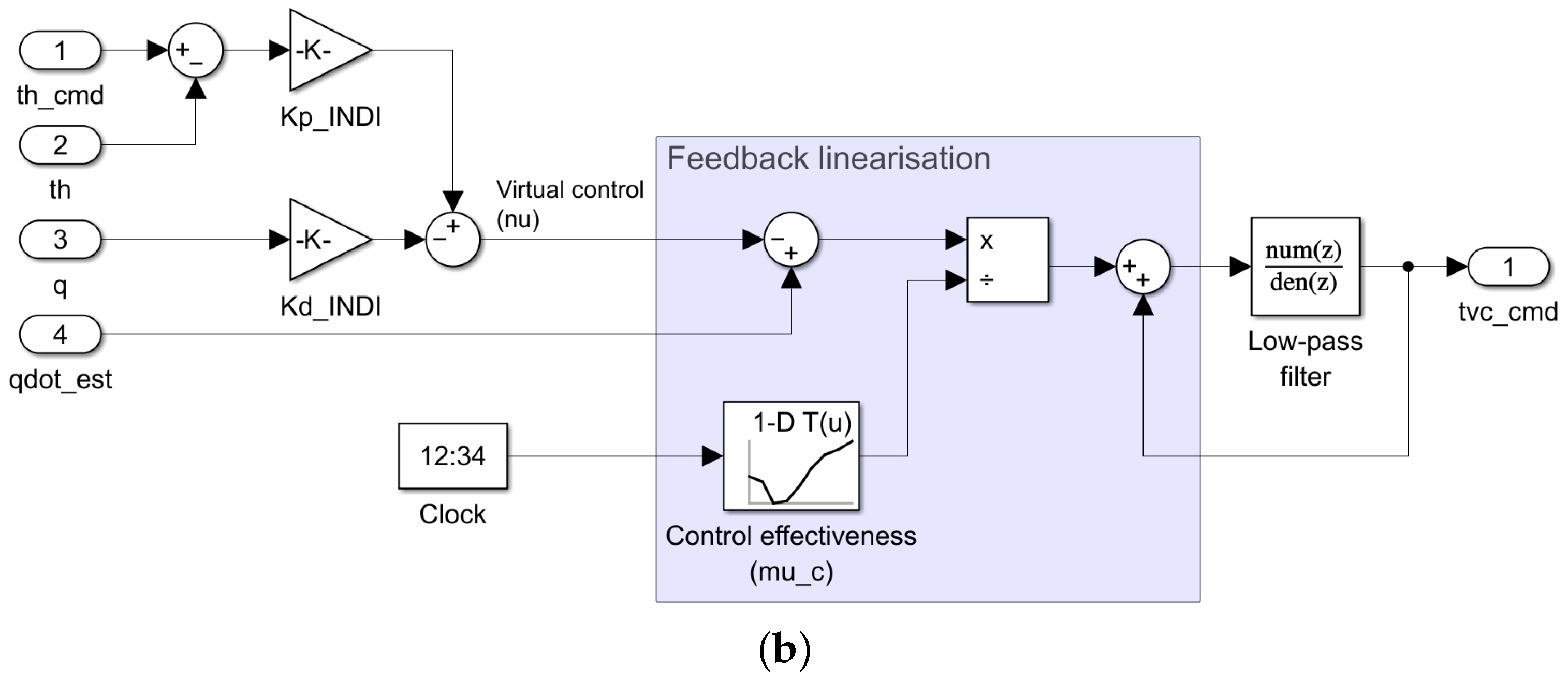
4.4. INDI Controller with Low-Pass Filter

When applied to the pure INDI controller developed in Section 4.2, the same tuning trade-off analysis showed a much smaller sensitivity to ${\omega }_{\dot{q}}$ but unacceptably high TVC rates. To address this issue, the INDI controller was augmented with a low-pass filter, as depicted in the right-hand side of Figure 3b. In this case, by taking the ${\beta }_0$ signal after the low-pass filter for the feedback linearisation, the unit delay used in Figure 3a is no longer necessary.

The outer linear gains and $\dot{q}$ estimation filter remain unchanged. The low-pass filter has bandwidth ${\omega }_{\beta }$ and a first-order structure as follows:

$$H_{\beta }\left(\mathrm{s}\right)={\displaystyle \frac{{\omega }_{\beta }}{\mathrm{s}+{\omega }_{\beta }}}$$

(42)

The purple line in Figure 4 shows the tuning trade-off using the INDI controller with low-pass filter and varying values of its bandwidth ${\omega }_{\beta }$. Compared with the PD controller with $\dot{q}$ feedback (blue line), the two controllers show a similar trend (i.e., smaller errors and larger TVC rates for higher bandwidths), yet the INDI controller leads to smaller TVC rates for the same level of error. As before, a more favourable trade-off would likely be achieved by using a higher-order low-pass filter, but this is outside the scope of this paper.

4.5. Control Design Summary

The four controllers in Section 4.1, Section 4.2, Section 4.3 and Section 4.4 were designed to enforce the same closed-loop properties throughout the flight. These are the characteristics:

• Natural frequency ${\omega }_{\theta }=2.5$ rad/s;
• Damping ratio $\zeta =0.8$;
• Steady-state error of 5%, i.e., $G_0=1.05$, only applicable to Section 4.3.

Furthermore, the bandwidth of the filters in Section 4.3 and Section 4.4, ${\omega }_{\dot{q}}$ and ${\omega }_{\beta }$, was tuned to provide the same pitch error in nominal conditions, as highlighted in Figure 4. The robust performance of these controllers is analysed in Section 5.

Table 2. Dependencies per control design method.

Control Design Method	Dependency on Model Parameters	Dependency on Measurements/Estimates
Scheduled PD	$J,l_{\mathrm{c}},T,C_{N_{\alpha }},l_{\alpha },\rho ,V$	$\theta ,q$
Scheduled PD with $\dot{q}$ feedback	$J,l_{\mathrm{c}},T,C_{N_{\alpha }},l_{\alpha },\rho ,V$	$\theta ,q,\dot{q}$
INDI with or without low-pass filter	$J,l_{\mathrm{c}},T$	$\theta ,q,\dot{q},\beta$

provides an overview of each controller’s dependency on the model parameters and sensor measurements/estimates. As anticipated, from the scheduled PD controller to the INDI controller, there is a progressive reduction in model dependency and an increased use of sensor information. More specifically, the INDI controller relies on measurements/estimates of $\dot{q}$ and $\beta$ to fully circumvent the knowledge of the aerodynamics model.

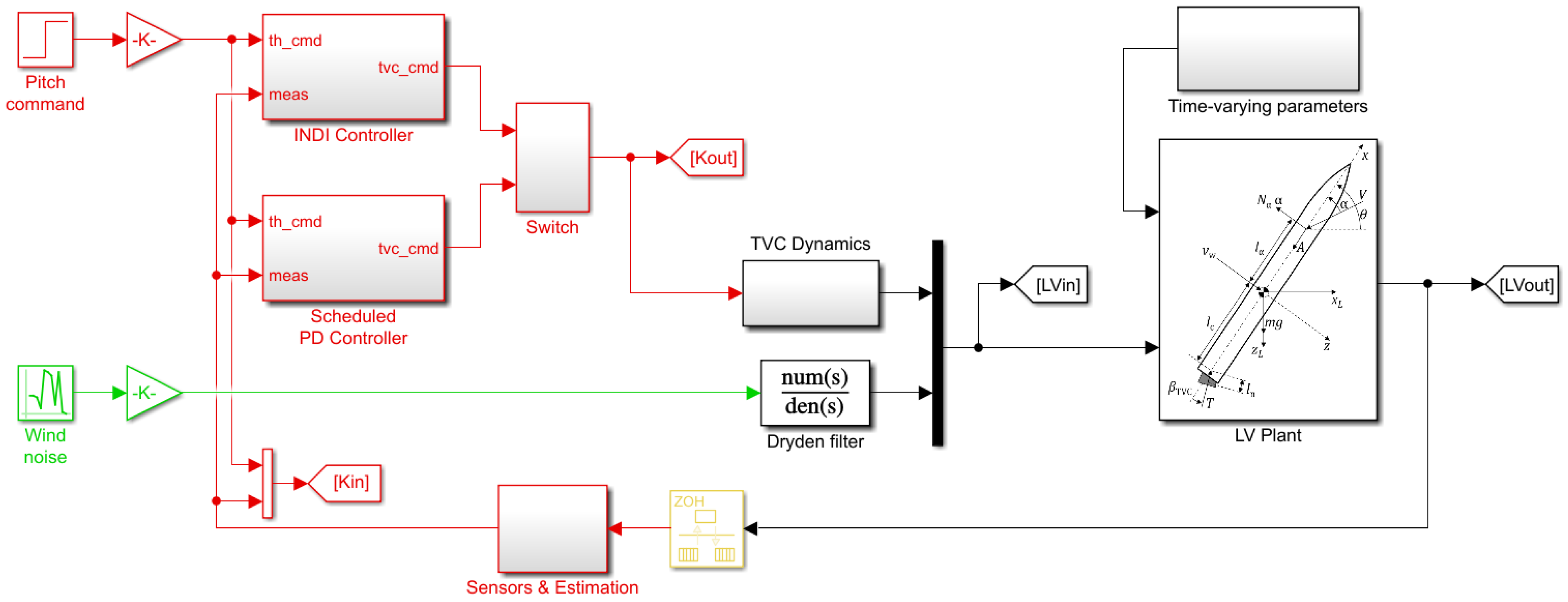
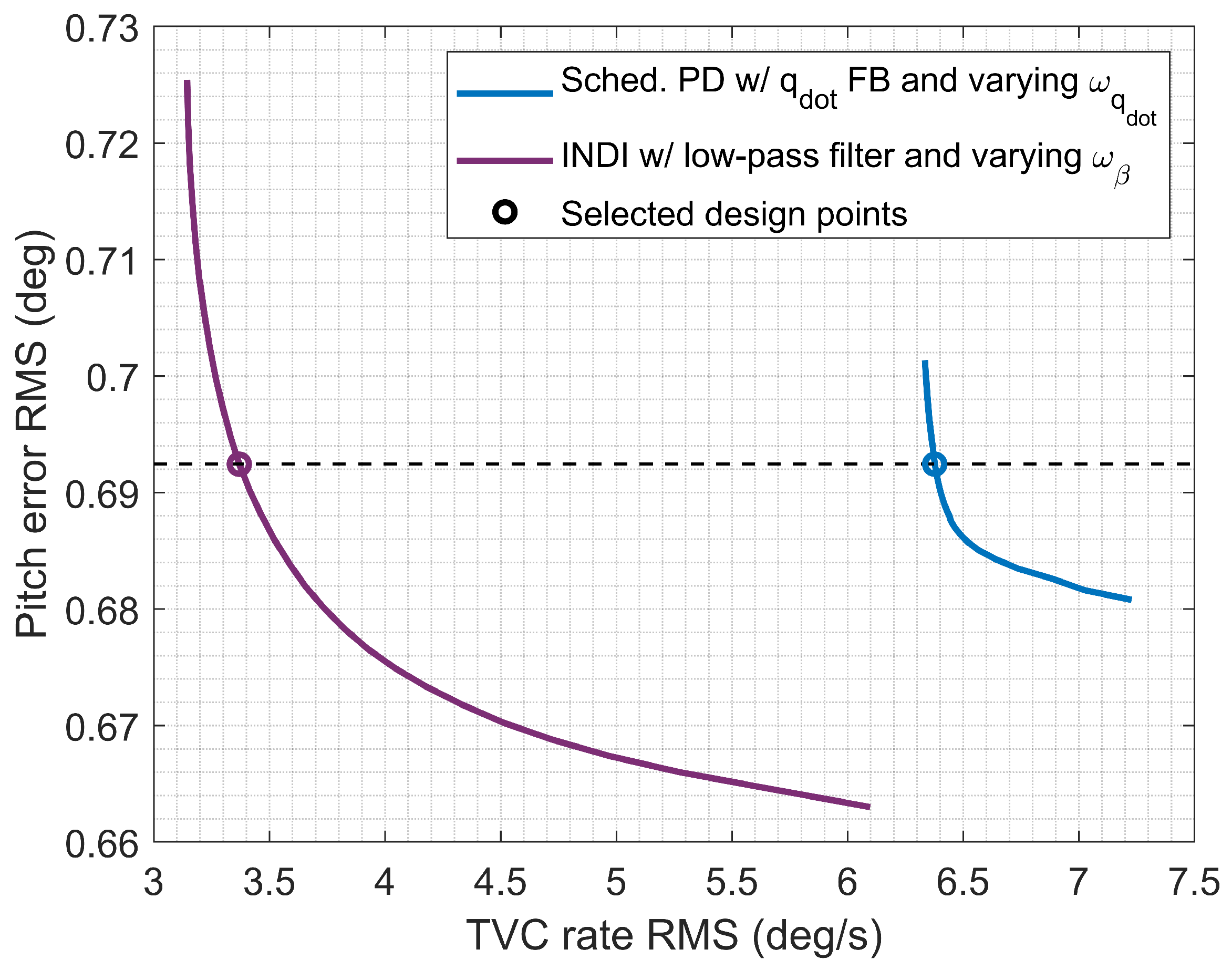
5. Time-Domain Robust Performance Analysis

This section analyses and compares the nonlinear time-domain performance the controllers developed in Section 4. Figure 5 shows dispersed responses of the $2^8=256$ corner cases within the uncertainty level of Table 1 when subjected to the same wind turbulence input $v_{\mathrm{w}}$, modelled as described in Section 3. From the top to the bottom rows, the figure depicts the obtained pitch error ${\theta }_{\mathrm{err}}$, TVC deflection $\beta$, and aerodynamic load indicator $Q\alpha$ along the trajectory. From left to right, the figure depicts results using the scheduled PD controller (Figure 5a, in black), scheduled PD controller with $\dot{q}$ feedback (Figure 5b, in blue), and INDI controller with low-pass filter (Figure 5c, in purple). The pure INDI controller (without low-pass filter) is not shown as it leads to unacceptably high TVC rates.

From Figure 5a,b, a reduction in the dispersion of all the indicators can be observed. This joint reduction clearly demonstrates the benefit of including $\dot{q}$ feedback in the control design. The pitch error (and partially the $Q\alpha$) is further reduced when using the INDI controller with low-pass filter, as depicted in Figure 5c, at the expense of higher TVC deflections (although still comparable to the pure PD controller). Note that $Q\alpha$ minimisation was not a specific control design objective in this case but comes as a direct consequence of smaller pitch and drift errors, as indicated in Equation (13b).

In order to visualise these trends more clearly, Figure 6a shows the wind response results using the same RMS ${\theta }_{\mathrm{err}}$ vs. $\dot{\beta }$ plot of Figure 4. Each point in Figure 6a corresponds to a single simulation from Figure 5. As anticipated, the pure PD controller (in black) provides the largest errors but the smallest TVC rates, while on the other hand, the pure INDI controller (in red) provides the smallest errors but the largest TVC rates. The PD controller with $\dot{q}$ feedback (in blue) and the INDI controller with low-pass filter (in purple) lie in between the two extremes, with the latter controller performing better than the former (i.e., with slightly smaller errors and TVC rates) but only marginally.

In order to complement the analysis, Figure 6b shows the same type of results for a step command in ${\theta }_{\mathrm{cmd}}$. As before, the pure PD controller (in black) leads by far to the largest errors and the pure INDI controller (in red) to the largest TVC rates. Performance in terms of error and TVC rate improves using either the PD controller with $\dot{q}$ feedback or the INDI controller with low-pass filter, and the difference between these two controllers is now more evident than for the wind responses.

In nominal conditions, it is known from Figure 4 that for the same error, the INDI controller with low-pass filter (in purple) provides a smaller TVC rate than the PD controller with $\dot{q}$ feedback (in blue). Nonetheless, Figure 6a shows that the former controller performs better also in terms of error, having a range of dispersion that is approximately four times smaller. The smaller error dispersion of the INDI controller with low-pass filter comes at the expense of a larger TVC rate dispersion, but its maximum value remains significantly lower than that of the PD controller with $\dot{q}$ feedback.

INDI-based controllers, by relying on angular acceleration and control input measurements/estimates, are known to be more sensitive to sensor noise and actuator delays than classical linear controllers. In order to assess this sensitivity, Figure 7 extends Figure 6a using the INDI controller with low-pass filter, showing wind simulation results with different combinations of the following:

• Gaussian noise on the angular rate signal, with $3\sigma =\left\{0,0.05,0.1\right\}$ deg/s, which affects the estimates of both q and $\dot{q}$ through Equation (34). Note that the $3\sigma$ value of 0.1 deg/s is considered to be very pessimistic [42].
• Time delay of $\left\{0,40,80\right\}$ ms on the signal commanded to the TVC actuator, corresponding to a delay of $\left\{0,1,2\right\}$ control samples.

From Figure 7, it can be observed that for the ranges considered, delays on the TVC signal have very little impact on the controller’s performance. Noise on the angular rate signal, on the other hand, leads to a more noticeable degradation, with the resulting TVC rates increasing approximately linearly with the noise variance.

This type of understanding is critical when designing and sizing INDI-based GNC software and hardware. The authors consider the scenario shown in the middle of Figure 7 (noise $3\sigma =0.05$ deg/s, TVC rate below 10 deg/s) to be very representative of a potential real-world application. The impact of angular rate noise would be minimised by using a higher-order-derivative filter $H_{\dot{q}}\left(\mathrm{s}\right)$ or by including an angular acceleration sensor in the GNC system.

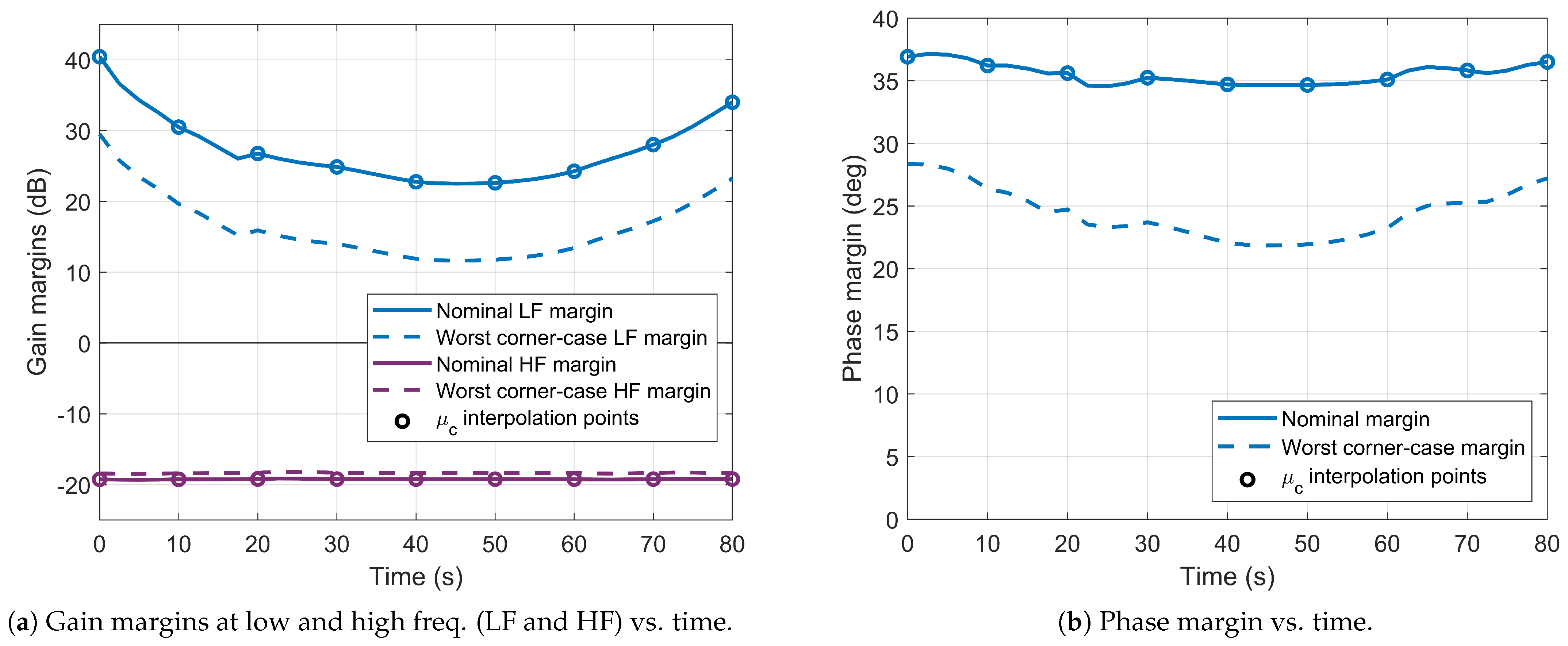
6. Frequency-Domain Robust Stability Analysis

Because of the nonlinear nature of INDI, attaining analytical proof of stability of INDI-based controllers [36] is much less trivial than for classical linear controllers. In order to mitigate this shortcoming, this section introduces a simple yet insightful frequency-domain approach to quantify stability degradation related to an imperfect feedback linearisation and to deviations from the control tuning conditions. This section is therefore focused on the controller developed in Section 4.4, not on a full comparison of controllers.

The proposed approach is based on linearised models of the nonlinear launcher simulator with the INDI control law in the loop at different flight conditions and on the fact that for a perfect feedback linearisation, the channel $\nu \left(\mathrm{s}\right)\to \theta \left(\mathrm{s}\right)$ behaves as a double integrator (recall Equation (32)). The INDI controller design was carried out under this assumption.

This approach was first presented in [37], but there was an error in the computation of the linearised models in that reference, which led to invalid stability analysis results. This section serves, therefore, as a correction of the results presented in [37].

Linearised models of $\nu \left(\mathrm{s}\right)\to \theta \left(\mathrm{s}\right)$ can be computed thanks to the following MATLAB^® (R2024b) routine

linearize(mdl, findop(mdl, t), …)

where mdl is the Simulink^® file instantiated with a certain configuration and t is the flight time instant. The analysis in this section considers the $2^8=256$ corner cases (within the uncertainty level of Table 1) and 33 instants (spaced every 2.5 s along the trajectory).

Figure 8a shows the frequency response of the aforementioned linearised models (in blue) together with the “perfect” double-integrator assumption (in red). This figure shows two important features:

• A dispersion of the linearised models, which is caused by deviations from the control tuning conditions due to the uncertain and time-varying nature of the model’s parameters;
• A mismatch between the linearised models and the double-integrator assumption, which grows in frequency ranges dominated by dynamical effects that are neglected in the feedback linearisation, i.e., drift motion at low frequencies (purple area) and TVC/TWD dynamics and $H_{\dot{q}}\left(\mathrm{s}\right)$ filter at high frequencies (blue area).

These models can be employed to assess the system’s stability margins when the loop is closed using Equation (36). To do so, it is convenient to plot the responses in a Nichols chart, which is depicted in Figure 8b for the nominal and corner-case samples. For a detailed explanation of the application of Nichols charts to launcher stability assessment, the reader is referred to [39].

The impact of the imperfect feedback linearisation on the system’s stability becomes evident in Figure 8b: the phase margin is reduced approximately by half and the system can be gain-destabilised, which is not the case under the double-integrator assumption. Nonetheless, all phase and gain margins remain substantial. When this is not the case, the linearised models of $\nu \left(\mathrm{s}\right)\to \theta \left(\mathrm{s}\right)$ can be employed instead of Equation (32) to re-tune the INDI outer control law. The stability margins are naturally driven by the value of ${\mu }_{\mathrm{c}}$, which is the main dependency of the INDI controller (recall Table 2). Accordingly, the margins become smaller for smaller values of ${\mu }_{\mathrm{c}}$ as the system’s control effectiveness decreases, and vice versa.

In order to assess the degradation caused by uncertainties and time variations, the gain and phase margins are plotted as a function of time in Figure 9a and b, respectively. Figure 9a contains the margins related to a reduction in gain (which impacts lower-frequency dynamics, often referred to as LF margin) in blue and to an increase in gain (which impacts higher-frequency dynamics, referred to as HF margin) in purple. The figures show the nominal margins in a continuous line, and the worst (minimum) corner-case margins (assuming the uncertainty level of Table 1) in a dashed line. The $N=9$ control tuning points, i.e., the interpolation nodes of ${\mu }_{\mathrm{c}}$, are indicated in the figures using circular marks. The main results are then summarised in

Table 3. Stability margin budget (gain margins are indicated in absolute value).

Case	LF Gain Margin (dB)	Phase Margin (deg)	HF Gain Margin (dB)
Double-integrator assumption	∞	69.84	∞
Nominal	22.62	34.66	19.21
Nominal with deviation from ${\mu }_{\mathrm{c}}$ interp. points	22.50	34.55	19.13
Worst-case	11.76	21.94	18.32
Worst-case with deviation from ${\mu }_{\mathrm{c}}$ interp. points	11.64	21.86	18.18

.

From Figure 9, it can be seen that the stability margins—especially the LF gain margin—show a noticeable variation over the flight, which follows the evolution of the launcher’s dynamic pressure. This variation is caused by the impact of drift motion at low frequencies (recall Figure 8a), which is neglected in the feedback linearisation and which is directly proportional to the dynamic pressure. The HF gain margin is significantly less sensitive to variations, as already anticipated from Figure 8b.

Between control tuning points, there is also a variation in margins due to mismatches between actual and interpolated values of ${\mu }_{\mathrm{c}}$. Nonetheless, this variation is extremely limited and leads to a degradation of around 0.1 deg and 0.1 dB, as can been seen from Table 3.

Stability degradation due to uncertainties is about two orders of magnitude higher, leading to margin losses (i.e., differences between nominal and worst-case values from Table 3) of 12.7 deg and 10.9 dB (at LF). In practice, the resulting stability margins must provide enough room to accommodate the impact of dynamical effects that were not considered in this study, such as flexible modes and noncollocated sensing. Nonetheless, the worst-case margins are plentiful, which suggests the feasibility of INDI-based launcher attitude control.

7. Extension to Launcher Control with Active Load Relief

The controllers analysed in Section 5 and Section 6 control only the attitude of the launcher, meaning that the lateral drift dynamics (Equation (11a)) can develop in an unbounded manner. One of the simplest approaches to control the drift motion is to augment the current design with an outer loop employing drift rate ($\dot{z}$) feedback. This section aims to showcase how such an approach can be effectively applied in conjunction with the INDI controller of Section 4.4.

The idea behind the proposed control law is to adjust the commanded pitch angle in the presence of drift motion so that when $\theta \to {\theta }_{\mathrm{cmd}}$ (which is ensured by the faster inner attitude controller), the induced angle of attack ${\alpha }_0$ is neutralised, i.e., ${\alpha }_0\to 0$. This leads then to an active minimisation of the induced aerodynamic load, quantified by $Q\alpha$.

The induced angle of attack is given by Equation (13b) without $v_{\mathrm{w}}$ since the wind speed is typically unknown (unless a wind estimator is included in the design [40]) and without the aerodynamic damping term due to the very high uncertainty in $l_{\alpha }/V$. This corresponds to

$${\alpha }_0=\theta +arctan{\displaystyle \frac{w}{V}}\approx \theta +{\displaystyle \frac{w}{V}}$$

(43)

where $w=\dot{z}$ is the drift rate. The pitch command is then scaled by a “load relief” gain $k_{LR}$ and by the normalised dynamic pressure $Q_{\mathrm{norm}}=Q/\max \left(Q\right)$, yielding the control law

$${\theta }_{\mathrm{cmd}}\left(\mathrm{s}\right)=-k_{LR}{\displaystyle \frac{Q_{\mathrm{norm}}}{V}}\dot{z}\left(\mathrm{s}\right)$$

(44)

This pitch command is then passed to the inner loop of Equation (36). The scaling by $Q_{\mathrm{norm}}$ guarantees that the load relief is tighter when the dynamic pressure is higher ($Q_{\mathrm{norm}}\to 1$) and more relaxed otherwise, allowing a tighter attitude tracking when the dynamic pressure is lower ($Q_{\mathrm{norm}}\to 0$ during the initial and final phases of the flight). Note that when $Q_{\mathrm{norm}}$ or $k_{LR}$ are zero, ${\theta }_{\mathrm{cmd}}\left(\mathrm{s}\right)=0$ and the outer loop is opened.

The implementation of Equation (44) is illustrated in Figure 10. A pre-computed grid of $Q_{\mathrm{norm}}\left[i\right]$ and $V\left[i\right]$ is employed to handle the variation of the model’s parameters throughout the flight (though $Q_{\mathrm{norm}}$ and V could alternatively be estimated from online measurements, similar to ${\mu }_{\mathrm{c}}$ in Figure 3).

A stepwise performance analysis of the proposed controller is provided in Figure 11. Each individual plot shows RMS values of different indicators (each point corresponding to a single simulation, similar to Figure 6) when using a different load relief gain $k_{LR}$, which is represented using different colours.

Figure 11a depicts dispersed results of $2^7=128$ corner cases per gain when subjected to the same wind input signal (these are the same conditions used in Section 5 except that the launcher’s mass is not dispersed now as its impact on the simulations is practically negligible). In Figure 11b, the launcher’s parameters are kept to their nominal values, but 128 scattered wind signals are tested per gain (this is important as wind disturbances have a major impact on the induced load). Then, Figure 11c shows the results using both uncertain parameters and scattered winds (amounting to $128\times 128=\mathrm{16,384}$ simulations per gain). From top to bottom, the rows of Figure 11 depict, respectively, ${\theta }_{\mathrm{err}}$ vs. $\dot{z}$, ${\theta }_{\mathrm{err}}$ vs. $Q\alpha$, and ${\theta }_{\mathrm{err}}$ vs. $\dot{\beta }$.

Starting with the first plot of Figure 11a, as $k_{LR}$ increases (from blue to purple), there is a significant reduction in drift rate at the expense of much higher pitch errors (due to the modified pitch command). The reduction in drift rate is then accompanied by a reduction in $Q\alpha$ (second plot), which is indeed the main aim of the designed outer-loop controller. The bottom plot shows that the impact of the load relief gain on the induced TVC rate is very little for smaller values of $k_{LR}$, but a few outliers are observed with $k_{LR}=9$, which indicates robustness issues for gains around this value. It should be noted that the higher pitch errors obtained in this case (maximum around 0.5 deg) remain comparable with what would be achieved using a traditional PD controller even without any load relief (maximum around 0.4 deg, from Figure 6a).

Figure 11b shows the same trade-off pitch error versus drift rate and $Q\alpha$, and it confirms that wind disturbances have a major impact: the plots depict much larger variations under dispersed winds than under uncertain parameters (Figure 11a). The only exception is the TVC rate, which shows very little sensitivity to the wind (bottom plot of Figure 11b).

Finally, Figure 11c illustrates the full dispersions caused by the combination of uncertain parameters and scattered winds. As can be seen, the conclusion concerning the trade-off pitch error versus drift rate and $Q\alpha$ through $k_{LR}$ remains valid. Specifically in terms of aerodynamic load (second plot), increasing $k_{LR}$ from 0 to 3 (from blue to yellow) has negligible impact on the minimum value of $Q\alpha$, but allows to reduce its worst-case value by 14.8% (from 92.3 to 78.6 kPa·deg), which proves the effectiveness of the proposed load relief approach. For $k_{LR}=9$, although the worst-case $Q\alpha$ is even lower, the robustness issues anticipated in the bottom plot of Figure 11a become too severe under wind dispersions, as observed in Figure 11c. Hence, the optimal choice of $k_{LR}$ shall be supported by a formal robustness analysis, which is similar to the one carried out for the inner attitude loop in Section 6 and therefore omitted for the sake of conciseness.

8. Conclusions

The results obtained in this study confirm that the Incremental Nonlinear Dynamic Inversion (INDI) technique provides a fast and robust launcher control design approach, which enables a stepwise transition from model-based to data-driven control design in the future. In particular, the results of a comprehensive nonlinear simulation campaign considering wind disturbances and parameter uncertainties indicate that the challenges associated with INDI-based control (e.g., sensitivity to sensor noise and actuator delay, difficulty of obtaining analytical proof of stability) are outweighed by the aforementioned benefits. Moreover, while being less disruptive than INDI, the linear control approach using angular acceleration feedback showed relevant performance improvements, and therefore, it also deserves consideration for a potential industrial application.

The outlook of this work is as follows: (1) furthering the suitability analysis of the INDI-based launcher control, (2) fine-tuning the components of the INDI architecture, and (3) fully exploiting the potential of this approach. For the first point, a thorough assessment of the impact of noncollocated sensing and flexible and sloshing modes needs to be carried out. The second point concerns the design of a better performing (higher-order) derivative filter and the combined tuning of the INDI gains and low-pass filter. As for the third point, the full exploitation of INDI will extend the current single-axis, single-TVC application to the multivariable case of controlling multiple axes (i.e., roll, pitch, and yaw) using multiple TVC actuators (potentially involving multiple engines).

References

1. Marcos, A.; Navarro-Tapia, D.; Simplício, P.; Bennani, S. Robust Control for Launchers: VEGA study case. J. Soc. Instrum. Control Eng. 2020, 3, 192–202. [Google Scholar]
2. Slotine, J.J.; Li, W. Applied Nonlinear Control; Prentice Hall Inc.: Hoboken, NJ, USA, 1990. [Google Scholar]
3. Khalil, H.K. Nonlinear Systems, 3rd ed.; Prentice Hall: Hoboken, NJ, USA, 2002. [Google Scholar]
4. Enns, D.; Bugajski, D.; Hendrick, R.; Stein, G. Dynamic inversion: An evolving methodology for flight control design. Int. J. Control 1994, 59, 71–91. [Google Scholar]
5. Reiner, J.; Balas, G.J.; Garrard, W.L. Flight Control Design Using Robust Dynamic Inversion and Time-scale Separation. Automatica 1996, 32, 1493–1504. [Google Scholar] [CrossRef]
6. Smith, P.R. A Simplified Approach to Nonlinear Dynamic Inversion Based Flight Control. In Proceedings of the AIAA Atmospheric Flight Mechanics Conference, Boston, MA, USA, 10–12 August 1998. [Google Scholar]
7. Looye, G. Design of Robust Autopilot Control Laws with Nonlinear Dynamic Inversion. at–Automatisierungstechnik 2001, 49, 523–531. [Google Scholar]
8. Lombaerts, T.J.; Huisman, H.O.; Chu, Q.P.; Mulder, J.A.; Joosten, D.A. Flight Control Reconfiguration based on Online Physical Model Identification and Nonlinear Dynamic Inversion. In Proceedings of the AIAA Guidance, Navigation, and Control Conference and Exhibit, Honolulu, HI, USA, 18–21 August 2008. [Google Scholar]
9. Bennani, S.; Looye, G. Flight Control Law Design for a Civil Aircraft using Robust Dynamic Inversion. In Proceedings of the IEEE/SMC CESA’98, Hammamet, Tunisia, 8–12 April 1998. [Google Scholar]
10. Smith, P.R.; Berry, A. Flight Test Experience of a Nonlinear Dynamic Inversion Control Law on the VAAC Harrier. In Proceedings of the AIAA Atmospheric Flight Mechanics Conference, Toronto, ON, Canada, 2–5 August 2000. [Google Scholar]
11. Bacon, B.J.; Ostroff, A.J. Reconfigurable Flight Control using Nonlinear Dynamic Inversion with a Special Accelerometer Implementation. In Proceedings of the AIAA Guidance, Navigation, and Control Conference and Exhibit, Providence, RI, USA, 16–19 August 2000. [Google Scholar]
12. Bacon, B.J.; Ostroff, A.J.; Joshi, S.M. Nonlinear Dynamic Inversion Reconfigurable Controller Utilizing a Fault-Tolerant Accelerometer Approach; Technical Report; NASA Langley Research Center: Hampton, VA, USA, 2000. [Google Scholar]
13. Bacon, B.J.; Ostroff, A.J.; Joshi, S.M. Reconfigurable NDI Controller using Inertial Sensor Failure Detection & Isolation. IEEE Trans. Aerosp. Electron. Syst. 2001, 37, 1373–1383. [Google Scholar]
14. Chen, H.B.; Zhang, S.G. Robust Dynamic Inversion Flight Control Law Design. In Proceedings of the ISSCAA 2008, 2nd International Symposium on Systems and Control in Aerospace and Astronautics, Shenzhen, China, 10–12 December 2008. [Google Scholar]
15. Sieberling, S.; Chu, Q.P.; Mulder, J.A. Robust Flight Control Using Incremental Nonlinear Dynamic Inversion and Angular Acceleration Prediction. J. Guid. Control Dyn. 2010, 33, 1732–1742. [Google Scholar] [CrossRef]
16. Simplício, P.; Pavel, M.; van Kampen, E.; Chu, Q.P. An Acceleration Measurements-based Approach for Helicopter Nonlinear Flight Control using Incremental Nonlinear Dynamic Inversion. Control Eng. Pract. 2013, 21, 1065–1077. [Google Scholar] [CrossRef]
17. Lu, P.; van Kampen, E.; Chu, Q.P. Robustness and Tuning of Incremental Backstepping Approach. In Proceedings of the AIAA Guidance, Navigation and Control Conference, Kissimmee, FL, USA, 5–9 January 2015. [Google Scholar]
18. Lu, P.; van Kampen, E. Active Fault-Tolerant Control System using Incremental Backstepping Approach. In Proceedings of the AIAA Guidance, Navigation and Control Conference, Kissimmee, FL, USA, 5–9 January 2015. [Google Scholar]
19. Smeur, E.J.; Chu, Q.P.; de Croon, G.C. Adaptive Incremental Nonlinear Dynamic Inversion for Attitude Control of Micro Air Vehicles. J. Guid. Control Dyn. 2016, 39, 450–461. [Google Scholar]
20. Smeur, E.J.; de Croon, G.C.; Chu, Q.P. Gust Disturbance Alleviation with Incremental Nonlinear Dynamic Inversion. In Proceedings of the IEEE/RSJ International Conference on Intelligent Robots and Systems (IROS), Daejeon, Republic of Korea, 9–14 October 2016. [Google Scholar]
21. Vlaar, C. Incremental Nonlinear Dynamic Inversion Flight Control. Master’s Thesis, Delft University of Technology, Faculty of Aerospace Engineering, Delft, The Netherlands, 2014. [Google Scholar]
22. Grondman, F.; Looye, G.; Kuchar, R.O.; Chu, Q.P.; van Kampen, E. Design and Flight Testing of Incremental Nonlinear Dynamic Inversion-based Control Laws for a Passenger Aircraft. In Proceedings of the AIAA Guidance, Navigation and Control Conference, Kissimmee, FL, USA, 8–12 January 2018. [Google Scholar]
23. Keijzer, T.; Looye, G.; Chu, Q.P.; van Kampen, E. Design and Flight Testing of Incremental Backstepping based Control Laws with Angular Accelerometer Feedback. In Proceedings of the AIAA SciTech Forum, San Diego, CA, USA, 7–11 January 2019. [Google Scholar]
24. Acquatella, B.P.; Falkena, W.; van Kampen, E.J.; Chu, Q.P. Robust Nonlinear Spacecraft Attitude Control Using Incremental Nonlinear Dynamic Inversion. In Proceedings of the AIAA Guidance, Navigation, and Control Conference, Minneapolis, MN, USA, 13–16 August 2012. [Google Scholar]
25. Acquatella B., P.; Chu, Q.P. Agile Spacecraft Attitude Control: An Incremental Nonlinear Dynamic Inversion Approach. IFAC-PapersOnLine 2020, 53, 5709–5716. [Google Scholar]
26. Acquatella B., P.; van Kampen, E.; Chu, Q.P. A Sampled-data Form of Incremental Nonlinear Dynamic Inversion for Spacecraft Attitude Control. In Proceedings of the AIAA SciTech Forum, San Diego, CA, USA, 3–7 January 2022. [Google Scholar]
27. Rickmers, P.; Bauer, W.; Stappert, S.; Sippel, M.; Redondo, Gutierrez, J.L.; Seelbinder, D.; Bernal, Polo, P.; Razgus, B.; Theil, S.; Acquatella, B.P.; et al. The Reusability Flight Experiment–ReFEx: From Design to Flight–Hardware. In Proceedings of the International Astronautical Congress (IAC), Dubai, United Arab Emirates, 25–29 October 2021. [Google Scholar]
28. Rickmers, P.; Kottmar, S.; Wibbels, G.; Bauer, W. ReFEx: Reusability Flight Experiment–A Demonstration Experiment for Technologies for Aerodynamically Controlled RLV Stages. In Proceedings of the Aerospace Europe Conference 2023–10th EUCASS–9th CEAS, Lausanne, Switzerland, 9–13 July 2023. [Google Scholar]
29. Redondo Gutierrez, J.L.; Seelbinder, D.; Theil, S.; Bernal Polo, P.; Gäßler, B.; Robens, J.; Acquatella, B.P. ReFEx: Reusability Flight Experiment–Architecture and Algorithmic Design of the GNC Subsystem. In Proceedings of the Aerospace Europe Conference 2023–10th EUCASS–9th CEAS, Lausanne, Switzerland, 9–13 July 2023. [Google Scholar]
30. Gäßler, B.; Robens, J. Incremental Nonlinear Dynamic Inversion Flight Control for the DLR Reusability Flight Experiment ReFEx. In Proceedings of the AIAA SciTech Forum, Kissimmee, FL, USA, 6–10 January 2025. [Google Scholar]
31. Mooij, E. Robust Control of a Conventional Aeroelastic Launch Vehicle. In Proceedings of the AIAA SciTech Forum, Orlando, FL, USA, 6–10 January 2020. [Google Scholar]
32. Mooij, E. Slosh Observer Design for Aeroelastic Launch Vehicles. In Proceedings of the AIAA SciTech 2020 Forum, Orlando, FL, USA, 6–10 January 2020. [Google Scholar] [CrossRef]
33. Mooij, E.; Wang, X. Incremental Sliding Mode Control for Aeroelastic Launch Vehicles with Propellant Slosh. In Proceedings of the AIAA SciTech 2021 Forum, Virtual, 11–15, 19–21 January 2021. [Google Scholar] [CrossRef]
34. Mooij, E. Dynamic Inversion Heat-Flux Tracking for Hypersonic Entry. In Proceedings of the AIAA SciTech Forum, National Harbor, MD, USA, 23–27 January 2023. [Google Scholar]
35. Mooij, E.; Wang, X. Nonlinear Robust Control and Observation for Aeroelastic Launch Vehicles with Propellant Slosh in a Turbulent Atmosphere. In Proceedings of the AIAA SciTech Forum, National Harbor, MD, USA, 23–27 January 2023. [Google Scholar] [CrossRef]
36. Wang, X.; van Kampen, E.; Chu, Q.P.; Lu, P. Stability Analysis for Incremental Nonlinear Dynamic Inversion Control. J. Guid. Control. Dyn. 2019, 42, 1116–1129. [Google Scholar] [CrossRef]
37. Simplício, P.; Acquatella, P.; Bennani, S. Launcher Attitude Control based on Incremental Nonlinear Dynamic Inversion: A Feasibility Study towards Fast and Robust Design Approaches. In Proceedings of the 12th International ESA Conference on Guidance, Navigation and Control Systems, Sopot, Poland, 12–16 June 2023. [Google Scholar]
38. Simplício, P.; Marcos, A.; Bennani, S. Reusable Launchers: Development of a Coupled Flight Mechanics, Guidance and Control Benchmark. J. Spacecr. Rocket. 2020, 57, 74–89. [Google Scholar] [CrossRef]
39. Simplício, P.; Bennani, S.; Marcos, A.; Roux, C.; Lefort, X. Structured Singular-Value Analysis of the Vega Launcher in Atmospheric Flight. J. Guid. Control. Dyn. 2016, 39, 1342–1355. [Google Scholar] [CrossRef]
40. Simplício, P.; Marcos, A.; Bennani, S. Launcher Flight Control Design using Robust Wind Disturbance Observation. Acta Astronaut. 2021, 186, 303–318. [Google Scholar] [CrossRef]
41. Navarro-Tapia, D.; Marcos, A.; Bennani, S.; Roux, C. Structured H-infinity and Linear Parameter Varying control design for the VEGA Launch Vehicle. In Proceedings of the the 7th European Conference for Aeronautics and Space Sciences, Milan, Italy, 3–6 July 2017. [Google Scholar]
42. Vandersteen, J.; Bennani, S.; Roux, C. Robust Rocket Navigation with Sensor Uncertainties: Vega Launcher Application. J. Spacecr. Rocket. 2018, 55, 153–166. [Google Scholar] [CrossRef]
Figure 1. Launcher model diagram.
Aerospace 12 00296 g001
Figure 2. Launcher simulator diagram.
Aerospace 12 00296 g002
Figure 3. INDI controllers’ implementation diagrams. (a) Pure INDI (from Section 4.2). (b) INDI with low-pass filter (from Section 4.4).
Aerospace 12 00296 g003aAerospace 12 00296 g003b
Figure 4. Tuning trade-off of angular acceleration feedback approaches.
Aerospace 12 00296 g004
Figure 5. Comparison of Monte Carlo wind responses using different controllers.
Aerospace 12 00296 g005
Figure 6. Overview of Monte Carlo results using different controllers.
Aerospace 12 00296 g006
Figure 7. Impact of sensor noise and actuator delays on INDI controller (with low-pass filter).
Aerospace 12 00296 g007
Figure 8. Frequency responses of linearised INDI-controlled plants for stability analysis.
Aerospace 12 00296 g008
Figure 9. Nominal and worst-case margins of INDI controller (with low-pass filter).
Aerospace 12 00296 g009
Figure 10. Outer-loop controller implementation diagram.
Aerospace 12 00296 g010
Figure 11. Time-domain performance analysis using varying load relief gains.
Aerospace 12 00296 g011