
Modeling Probabilistic Safety Margins in Convective Weather Avoidance Within European Airspace


Abstract
1. Introduction
2. Background
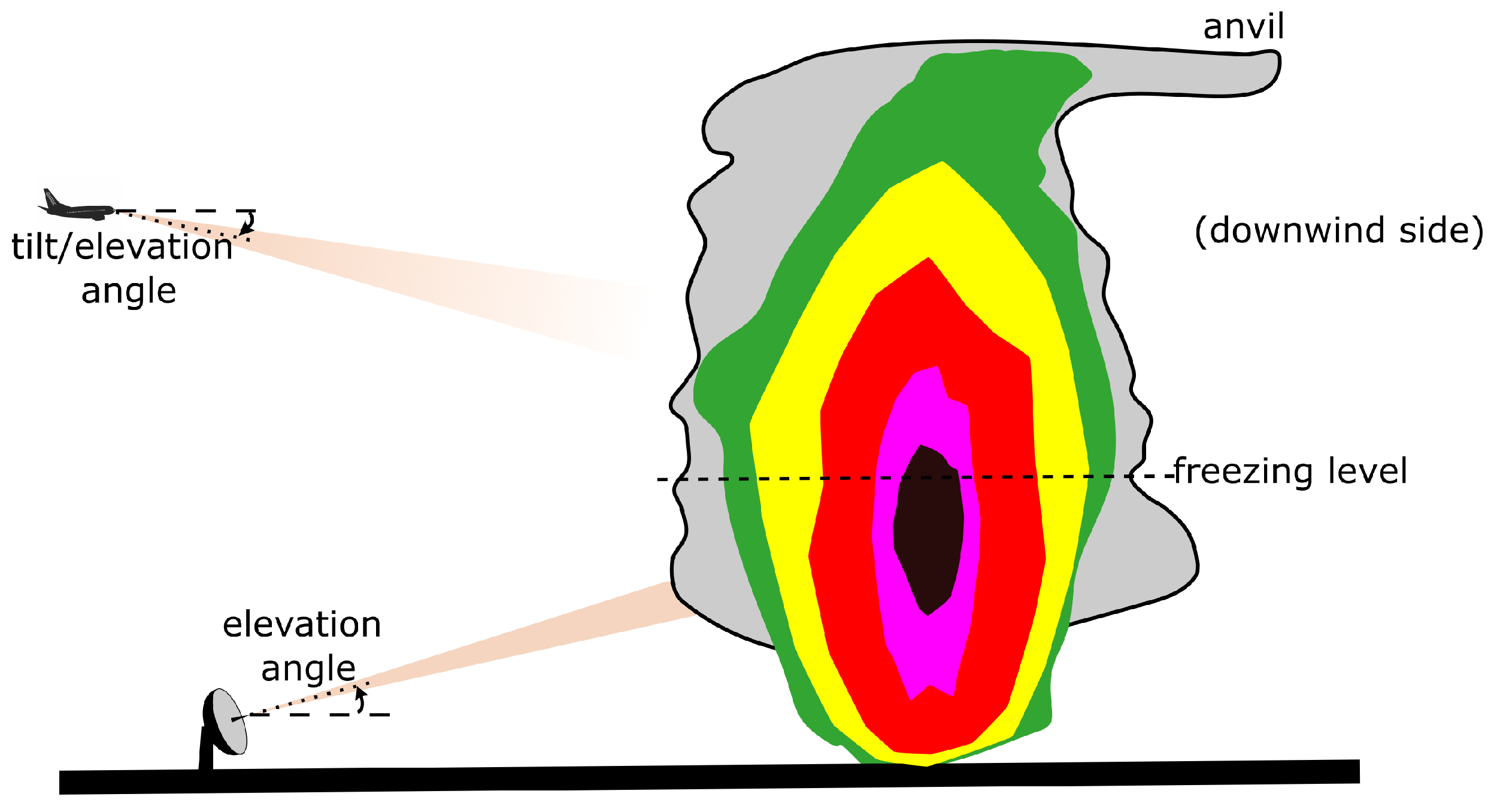
2.1. Basic Weather Radar Principles and General Characteristics
2.2. Related Works on Characterizing Lateral Deviations due to Convective Weather
3. Methodology
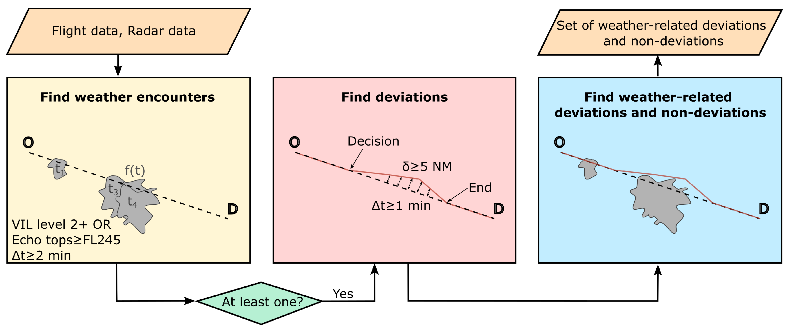
3.1. Detection of Weather-Related Deviations
- For each time interval with a meteorological picture, extract the polygons of the weather areas, label them, and trim the flight trajectories for the interval.
- Compute the intersections between the trimmed trajectories and labeled polygons, determining entry and exit points and times.
- Repeat the process for every time interval of interest.
- Organize the results so that the sequence of encounters for each flight can be analyzed.
- For each flight, merge consecutive periods within a polygon, which correspond to weather updates.
- Check whether closely spaced encounters for each flight can be merged, using a threshold of one minute.
- Discard weather encounters lasting less than two minutes.
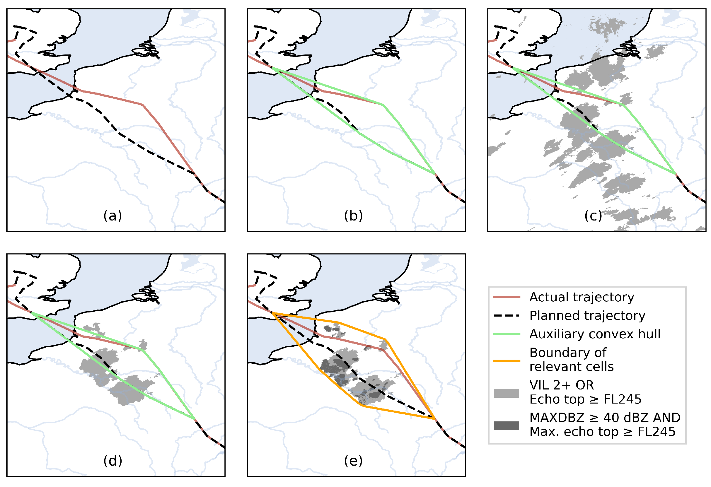
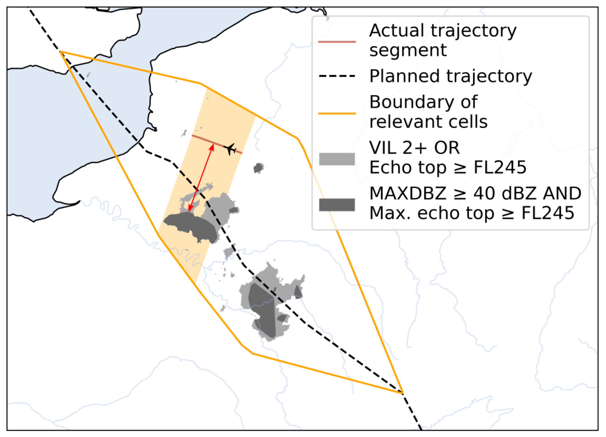
3.2. Calculation of Lateral Margins
- Compute the convex hull that encompasses all points in both the actual and planned trajectory from the decision point to the end point.
- Determine the maximum time interval for the weather data, defined by the period from the earliest decision point (either actual or planned) to the latest end point (either actual or planned).
- Identify all weather areas during the period determined in Step 2, and intersect with the convex polygon determined in Step 1.
- Compute a new convex hull that encompasses both the initial convex polygon and all the weather areas identified in Step 3.
3.3. Determination of Safety Margins. The Proposed Model
3.4. Assessment of the Probabilistic Safety Margins
4. Case Study
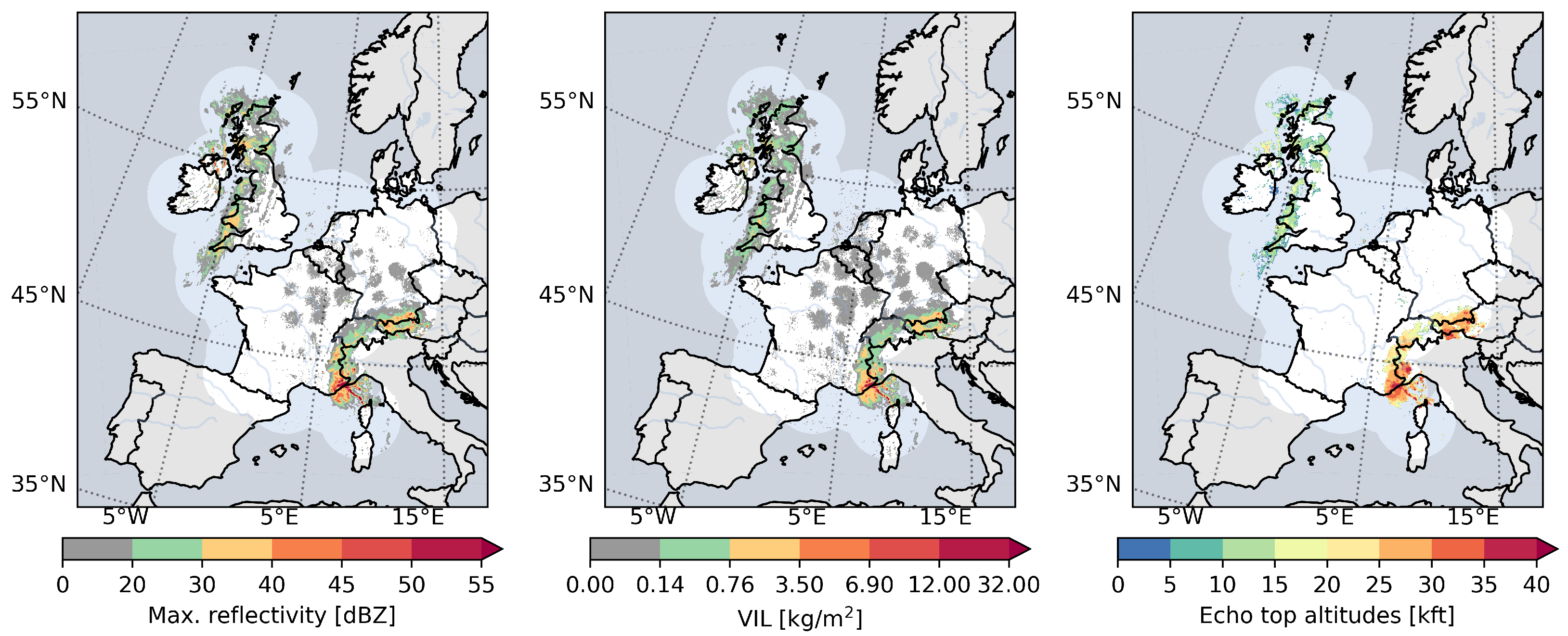
4.1. Weather Radar Data
4.2. Traffic Data
- Point removal: eliminated records affected by on-ground status, NaN values, duplicate entries, or spatiotemporal outliers.
- Unpaired flight legs: detected and removed flight legs that could not be matched with planned trajectories.
- Weather radar coverage: discarded points located outside the radar coverage area.
- Gap identification: identified gaps where the distance between consecutive waypoints exceeded 30 km. Trajectories with such gaps were split, treating each piece of trajectory independently.
- Flight filtering: removed flights or trajectory pieces that did not meet a minimum duration of 15 min or contained at least 30 waypoints.
- Trajectory association: matched each resulting piece of actual trajectory with the closest piece of the corresponding planned trajectory.
5. Results
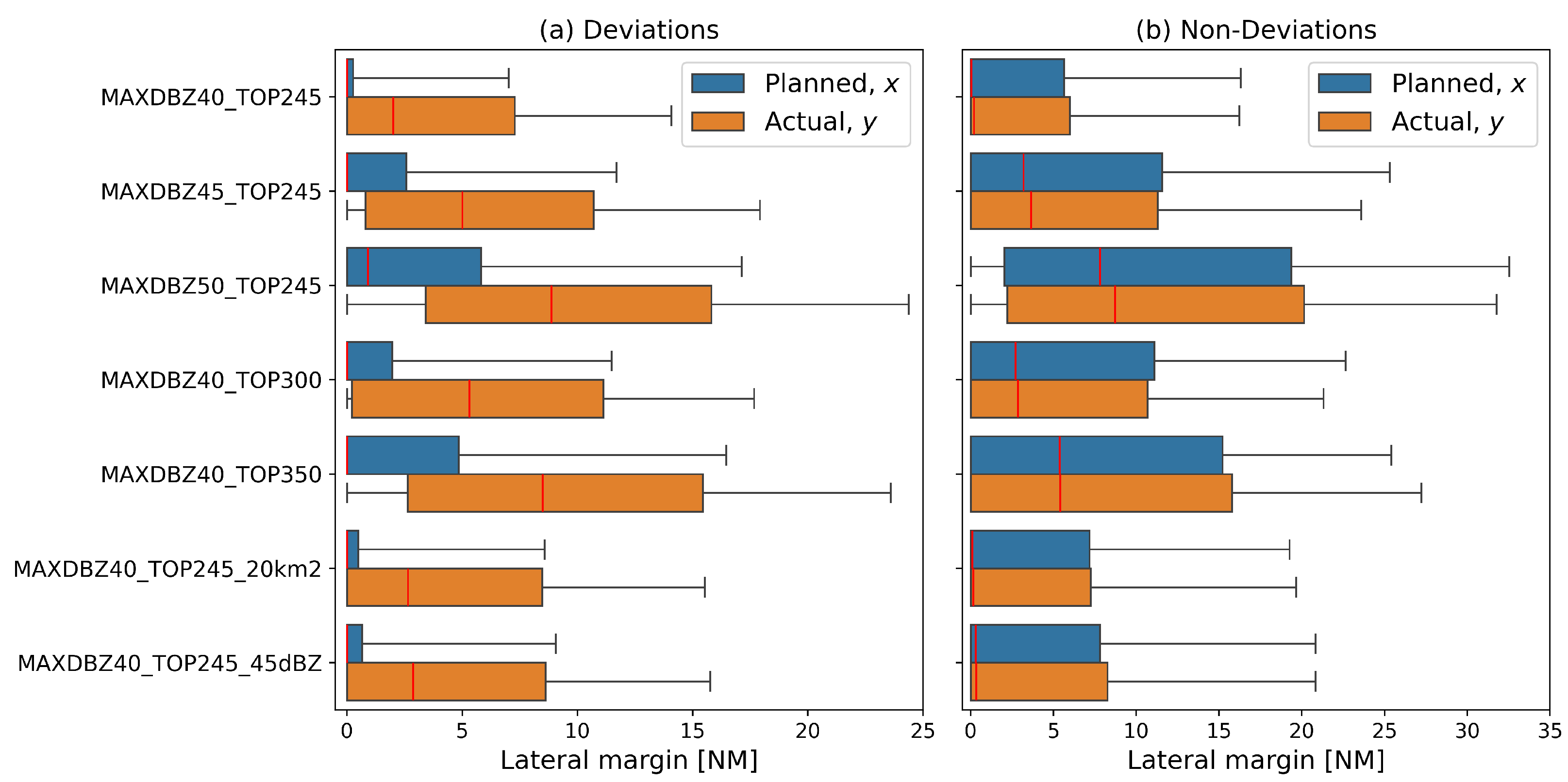
5.1. Analysis of Historical Lateral Margins
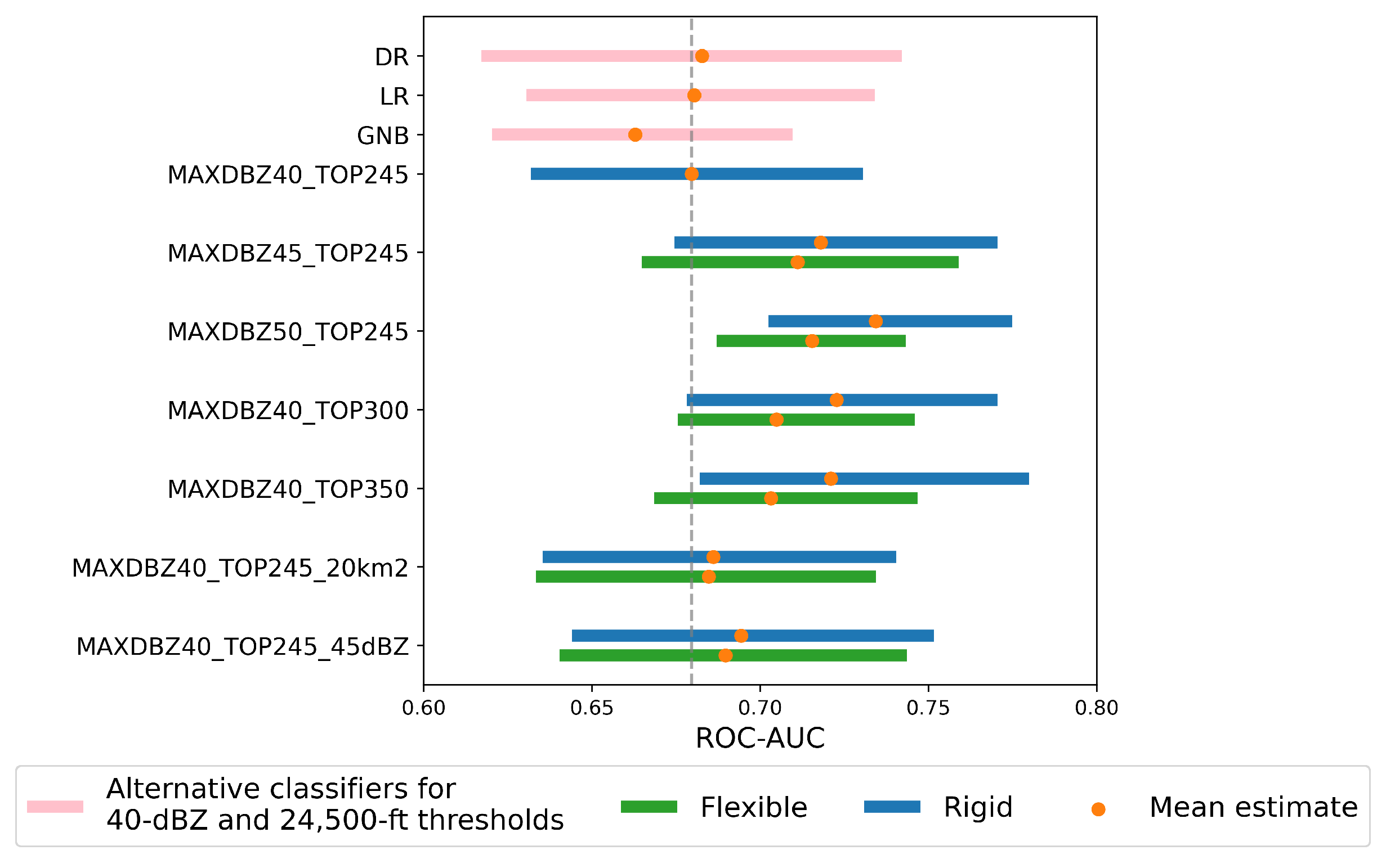
5.2. Assessment of Decision-Making Predictions
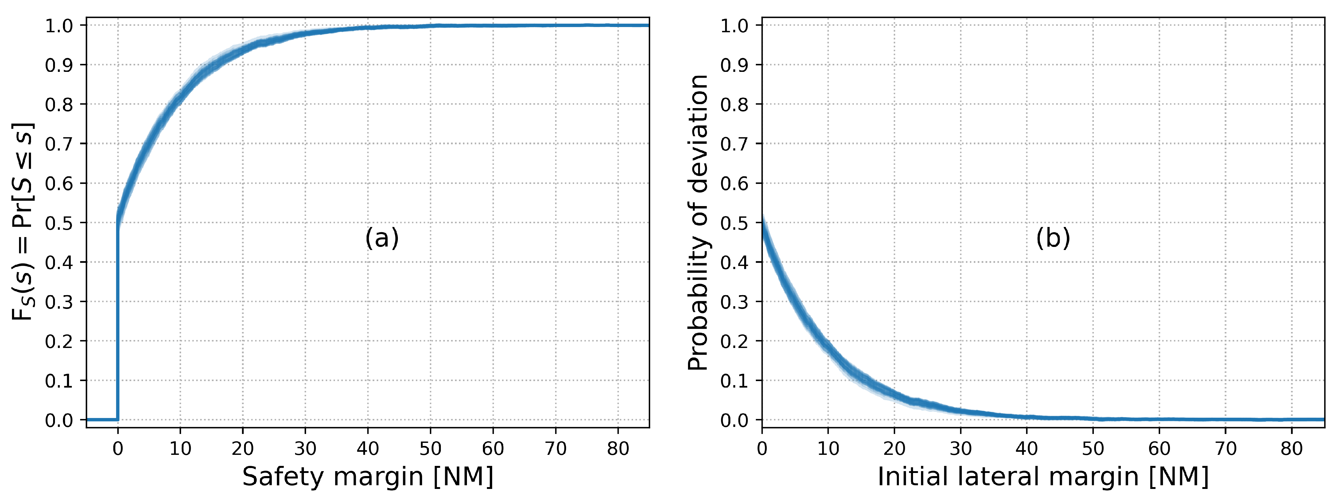
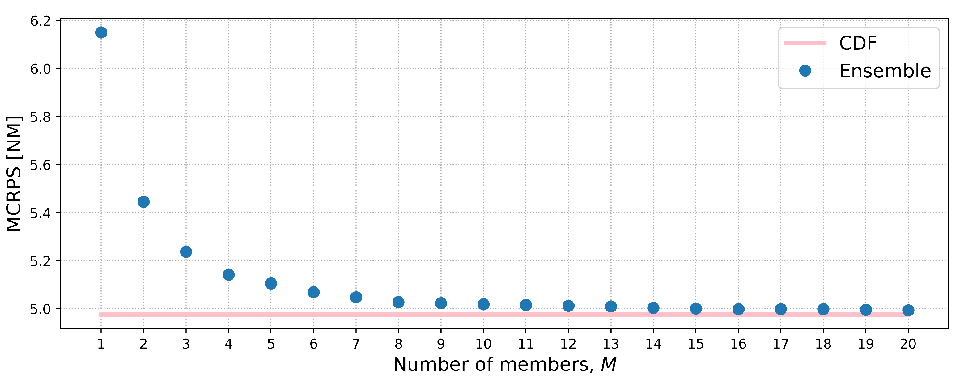
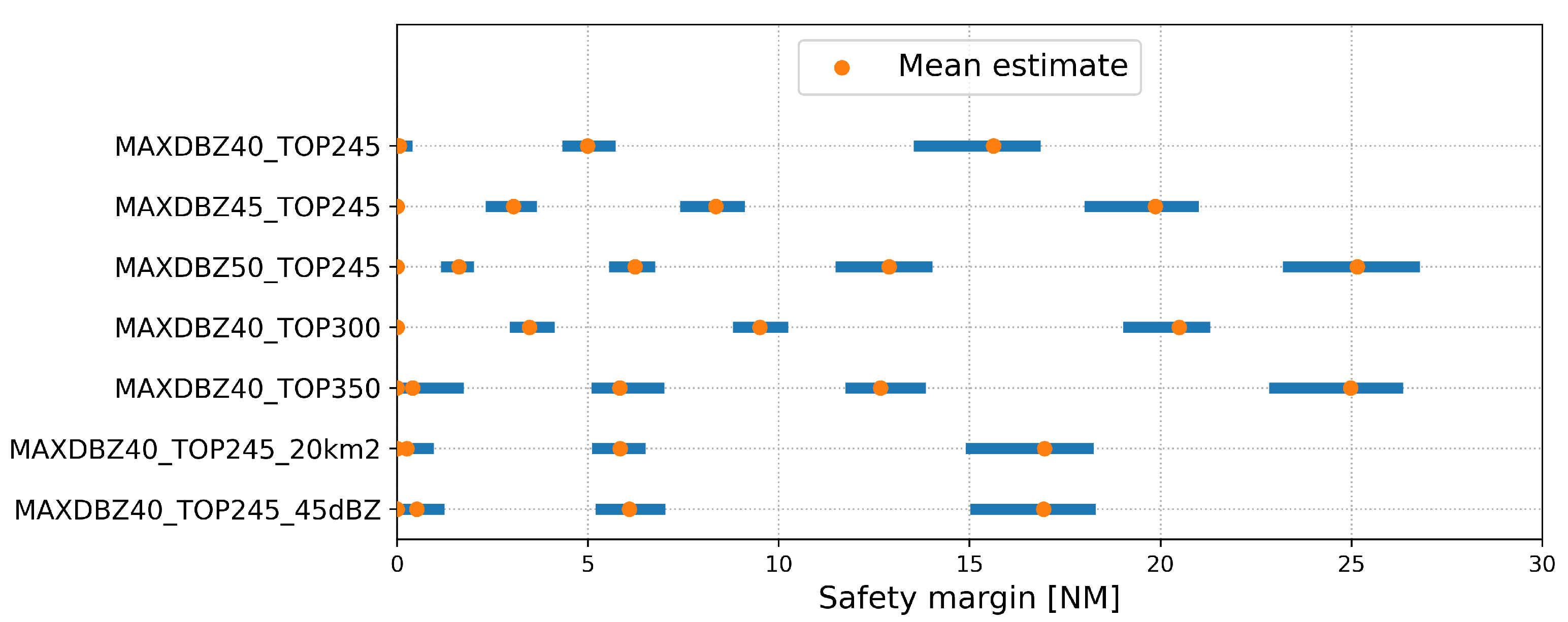
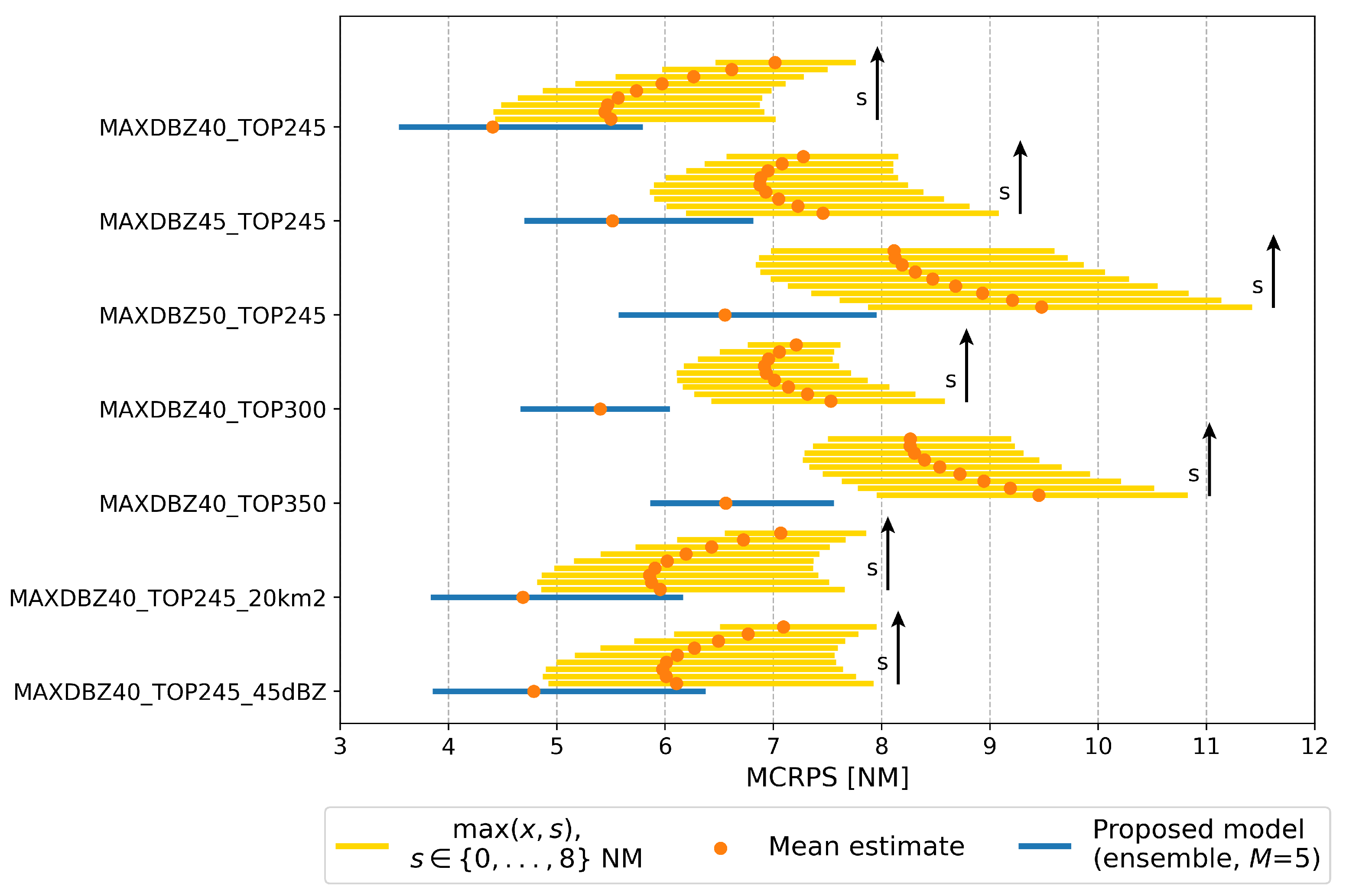
5.3. Assessment of Probabilistic Safety Margins
6. Conclusions
Author Contributions
Funding
Data Availability Statement
Acknowledgments
Conflicts of Interest
Abbreviations
| ATFM | Air traffic flow management |
| CDF | Cumulative distribution function |
| CRPS, MCRPS | Continuous ranked probability score, Mean CRPS |
| DR | Decision rule |
| GNB | Gaussian naïve Bayes |
| LR | Logistic regression |
| ROC-AUC | Area under the receiver Operating Characteristic curve |
| VIL | Vertically integrated liquid |
| VIP | Video integrator and processor |
| Nomenclature | |
| Cumulative distribution function | |
| M | Number of ensemble members |
| Dataset sizes for training and validation, respectively | |
| Probability | |
| Stochastic and deterministic safety margin, respectively | |
| Random variable representing the initial lateral margin | |
| and its realization, respectively | |
| Random variable representing the final lateral margin, its realization, | |
| and its estimation, respectively | |
| Subscripts | |
| i | scenario i |
| k | summation index |
| Superscripts | |
| j | ensemble member j |
Appendix A
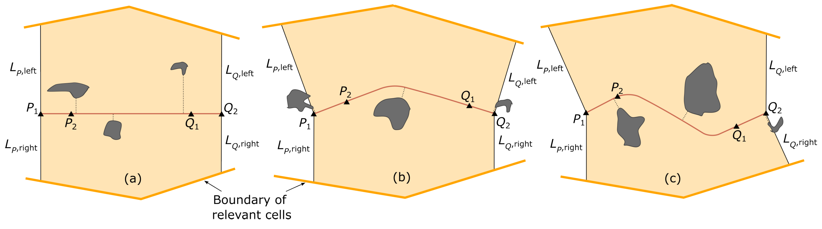
- Let and denote the first and second waypoints, respectively, of the trajectory segment within the time interval and and denote the second-to-last and last waypoints, respectively. Compute the course directions , , and of the segments , , and , respectively.
- Calculate the rhumb line . If , originates at and extends with a constant course of 90° until it intersects the boundary of the relevant cells. Conversely, if , the rhumb line originates at and extends with a constant course of 90° until it intersects the boundary of the relevant cells.
- Calculate the rhumb line . If , originates at and extends with a constant course of 90° until it intersects the boundary of the relevant cells. Conversely, if , the rhumb line originates at and extends with a constant course of 90° until it intersects the boundary of the relevant cells.
- Calculate the rhumb line . If , originates at and extends with a constant course of 90° until it intersects the boundary of the relevant cells. Conversely, if , the rhumb line originates at and extends with a constant course of 90° until it intersects the boundary of the relevant cells.
- Calculate the rhumb line . If , originates at and extends with a constant course of 90° until it intersects the boundary of the relevant cells. Conversely, if , the rhumb line originates at and extends with a constant course of 90° until it intersects the boundary of the relevant cells.
- Define the stripe as the area delimited by rhumb lines , , , , and the boundary of relevant cells.
References
- FAA; US Department of Transportation. Thunderstorms. In Aviation Weather Handbook; Academics, A.S., Ed.; Aviation Supplies & Academics, Inc.: Newcastle, WA, USA, 2022; Chapter 22; pp. 21–22. Available online: https://www.faa.gov/documentLibrary/media/Order/FAA-H-8083-28_Order_8083.28.pdf (accessed on 15 October 2023).
- EASA. The launch edition. In Conversation Aviation; EASA: Cologne, Germany, 2023; p. 37. Available online: https://www.easa.europa.eu/community/system/files/2023-03/Conversation%20Aviation%20-%2001%202023.pdf (accessed on 15 October 2023).
- FAA. Safety of Flight. In Aeronautical Information Manual; Aviation Supplies & Academics, Inc.: Newcastle, WA, USA, 2024; Chapter 7; p. 7-1-26. Available online: https://www.faa.gov/air_traffic/publications/atpubs/aim_html/chap7_section_1.html (accessed on 15 October 2023).
- FAA. Thunderstorms—Don’t flirt...skirt ’em. In FAA Safety Team; Flight Safety Foundation: Alexandria, VA, USA, 2008; p. 2. Available online: https://www.faasafety.gov/files/gslac/library/documents/2011/Aug/56397/FAA%20P-8740-12%20Thunderstorms[hi-res]%20branded.pdf (accessed on 15 October 2023).
- Air Accident Investigation Branch (UK). Airbus A321-231, G-MIDJ; Technical Report; U.K. Department for Transport: Farnborough, UK, 2004; p. 16. [Google Scholar]
- National Air Traffic Services (UK). The Effect of Thunderstorms and Associated Turbulence on Aircraft Operations; Civil Aviation Authority: Hounslow, UK, 2010; pp. 4, 8. [Google Scholar]
- Willett, J.; Merceret, F.; Krider, P.; O’Brien, P.; Dye, J.; Walterscheid, R.; Stolzenburg, M.; Cummins, K.; Christian, H.; Madura, J. Rationales for the lightning launch commit criteria; Technical Report; NASA: Washington, DC, USA, 2016; pp. 30, 36–70. [Google Scholar]
- Marconnet, D.; Norden, C.; Vidal, L. Optimum Use of Weather Radar. In Safety First; Airbus S.A.S: Washington, DC, USA, 2016; pp. 7–12, 20. Available online: https://mms-safetyfirst.s3.eu-west-3.amazonaws.com/pdf/safety+first/optimum-use-of-weather-radar.pdf (accessed on 27 October 2023).
- ECA. Pilots’ Vision on Weather; SESAR JU: Brussels, Belgium, 2014. Available online: https://www.eurocockpit.eu/sites/default/files/2017-04/Pilots%27%20Vision%20on%20Weather%202014_0.pdf (accessed on 18 April 2024).
- ECA. Weather Information to Pilots Strategy Paper; EASA: Cologne, Germany, 2018. Available online: https://www.easa.europa.eu/sites/default/files/dfu/EASA-Weather-Information-to-Pilot-Strategy-Paper.pdf (accessed on 11 April 2024).
- EASA. European Plan for Aviation Safety (EPAS) Volume II—EPAS Actions; Technical Report; EASA: Cologne, Germany, 2024; pp. 19–20. [Google Scholar]
- EASA. Aviation Authorities’ Research Agenda; Technical Report; EASA: Cologne, Germany, 2024; pp. 25–26. [Google Scholar]
- Barber, K.; Mullendore, G. The Importance of Convective Stage on Out-of-Cloud Convectively Induced Turbulence from High-Resolutions Simulations. Mon. Wea. Rev. 2020, 148, 4587–4605. [Google Scholar] [CrossRef]
- Honeywell. Honeywell RDR-7000 Weather Radar: A ’No Brainer’ for Global XRS Pilot Honeywell International, Inc.: Phoenix, AZ, USA. 2020. Available online: https://www.honeywell.com/content/dam/honeywellbt/en/documents/downloads/hon-corp-honeywell-rdr-7000-weather-radar-a-no-brainer-for-global-xrs-pilot.pdf (accessed on 7 June 2024).
- Collins Aerospace. WXR-2100 MultiScan ThreatTrack™ Weather Radar. 2022. Available online: https://www.collinsaerospace.com/what-we-do/industries/commercial-aviation/flight-deck/surveillance/weather-radar/wxr-2100-multiscan-threat-track-weather-radar (accessed on 7 June 2024).
- Rubnich, M.; DeLaura, R. An Algorithm to Identify Robust Convective Weather Avoidance Polygons in En Route Airspace. In Proceedings of the 10th AIAA Technology, Integration, and Operations Conference, Forth Worth, TX, USA, 13–15 September 2010. [Google Scholar]
- Ison, D. Navigating Weather: A Pilot’s Guide to Airborne and Datalink Weather Radar; Aviation Supplies & Academics: Newcastle, WA, USA, 2021; Chapter 2, 3; ISBN 978-1644251249. [Google Scholar]
- García-Heras, J.; Soler, M.; González-Arribas, D.; Eschbacher, K.; Rokitansky, C.; Sacher, D.; Gelhardt, U.; Lang, J.; Hauf, T.; Simarro, J.; et al. Robust flight planning impact assessment considering convective phenomena. Transp. Res. Part C Emerg. 2021, 123, 102968. [Google Scholar] [CrossRef]
- Andrés, E.; García-Heras, J.; González, D.; Soler, M.; Radišić, T.; Andraši, P.; Valenzuela, A.; Franco, A.; Nunez-Portillo, J.; Rivas, D. Probabilistic Analysis of Air Traffic in Adverse Weather Scenarios. In Proceedings of the 10th International Conference on Research in Air Transportation (ICRAT), Tampa, FL, USA, 19–23 June 2022. [Google Scholar]
- Krozel, J.; Mitchell, J.; Polishchuk, V.; Prete, J. Capacity Estimation for Airspaces with Convective Weather Constraints. In Proceedings of the AIAA Guidance, Navigation and Control Conference and Exhibit, Hilton Head, SC, USA, 20–23 August 2007. [Google Scholar] [CrossRef]
- FAA-ATO; Eurocontrol; European Commission. Comparison of Air Traffic Management Related Operational and Economic Performance; Technical Report; FAA-ATO System Operations Services and EUROCONTROL AIU: Blagnac, France, 2024. [Google Scholar]
- Enea, G.; Reynolds, T.; Venuti, J.; Polishchuk, T.; Polishchuk, V.; Lemetti, A.; Lau, A.; Solzer, J.; Bölle, T. Comparing Convective Weather Impacts on Air Traffic Management Operations in United States, Canada & Europe. In Proceedings of the 34th Congress of the International Council of the Aeronautical Sciences, Florence, Italy, 9–13 September 2024. [Google Scholar]
- Taszarek, M.; Allen, J.; Púčik, T.; Hoogewind, K.A.; Brooks, H.E. Severe Convective Storms across Europe and the United States. Part II: ERA5 Environments Associated with Lightning, Large Hail, Severe Wind, and Tornadoes. J. Clim. 2020, 33, 10263–10286. [Google Scholar] [CrossRef]
- Rigo, T.; Farnell, C. Evaluation of the Radar Echo Tops in Catalonia: Relationships with Severe Weather. Remote. Sens. 2022, 14, 6265. [Google Scholar] [CrossRef]
- Eurocontrol. Climate Change Risks for European Aviation 2021. Annex 2: Impact of Changes in Storm Patterns and Intensity on Flight Operations; Technical Report; EUROCONTROL: Brussels, Belgium, 2021; pp. 33–43, 54–55. [Google Scholar]
- Eurocontrol. Forecast Update 2024–2030—Spring 2024; Technical Report; EUROCONTROL: Brussels, Belgium, 2024. [Google Scholar]
- Airbus. Severe Weather Hazards: The Best Is to Anticipate and Avoid. 2024. Available online: https://www.airbus.com/en/newsroom/stories/2024-07-severe-weather-hazards-the-best-is-to-anticipate-and-avoid (accessed on 9 July 2024).
- Saltikoff, E.; Haase, G.; Delobbe, L.; Gaussiat, N.; Martet, M.; Idziorek, D.; Leijnse, H.; Novák, P.; Lukach, M.; Stephan, K. OPERA the Radar Project. Atmosphere 2019, 10, 320. [Google Scholar] [CrossRef]
- Huber, M.; Trapp, J. A Review of NEXRAD Level II: Data, Distribution, and Applications. J. Terr. Obs. 2009, 1, 4. Available online: https://docs.lib.purdue.edu/cgi/viewcontent.cgi?article=1042&context=jto (accessed on 24 October 2024).
- National Transportation Safety Board. Actual Age of NEXRAD Data Can Differ Significantly From Age Indicated on Display. 2015. Available online: https://www.ntsb.gov/Advocacy/safety-alerts/Documents/SA-017.pdf (accessed on 24 October 2024).
- Berberi, L. Maltempo a Milano, la grandine buca il muso dell’aereo diretto a New York: Volo dirottato a Roma. 2023. Available online: https://www.corriere.it/economia/consumi/23_luglio_24/maltempo-milano-grandine-buca-muso-dell-aereo-diretto-new-york-volo-dirottato-roma-8495fe2c-2a32-11ee-84ae-fdab1efa7b6b.shtml (accessed on 24 July 2024).
- Chang, S.; Deng, Y.; Zhang, Y.; Zhao, Q.; Wang, R.; Zhang, K. An Advanced Scheme for Range Ambiguity Suppression of Spaceborne SAR Based on Blind Source Separation. IEEE Trans. Geosci. Remote. Sens. 2022, 60, 5230112. [Google Scholar] [CrossRef]
- Greene, D.; Clark, R. Vertically Integrated Liquid Water – A New Analysis Tool. Mon. Wea. Rev. 1972, 100, 548–552. [Google Scholar] [CrossRef]
- Robinson, M.; Evans, J.; Crowe, B. En Route Weather Depiction Benefits of the NEXRAD Vertically Integrated Liquid Water Product utilized by the Corridor Integrated Weather System. In Proceedings of the 10th Conference on Aviation Range and Aerospace Meteorology, Portland, OR, USA, 12 May 2002; pp. 120–123. [Google Scholar]
- Crowe, B.; Miller, D. The Benefits of Using NEXRAD Vertically Integrated Liquid Water as an Aviation Weather Product. In Proceedings of the 8th Conference on Aviation Range and Aerospace Meteorology, Dallas, TX, USA, 10–15 January 1999. [Google Scholar]
- ICAO. Doc 8896—Manual of Aeronautical Meteorological Practice; ICAO: Montreal, QC, Canada, 2021; p. A8-7. [Google Scholar]
- Hallowell, R.; Wolfson, M.; Forman, B.; Moore, M.; Rotz, T.; Miller, D.; Carty, C.; McGettigan, S. The Terminal Convective Weather Forecast Demonstration at the DFW International Airport. In Proceedings of the 8th Conference on Aviation Range and Aerospace Meteorology, Dallas, TX, USA, 10–15 January 1999. [Google Scholar]
- Temme, M.; Tienes, C. Factors for Pilot’s Decision Making Process to Avoid Severe Weather during Enroute and Approach. In Proceedings of the 2018 IEEE/AIAA 37th Digital Avionics Systems Conference (DASC), London, UK, 23–27 September 2018; pp. 1–10. [Google Scholar]
- Lewis, T.; Burke, K.; Underwood, M.; Wing, D. Weather Design Considerations for the TASAR Traffic Aware Planner. In Proceedings of the AIAA Aviation 2019 Forum, Dallas, TX, USA, 17–21 June 2019. [Google Scholar]
- Benson, L. Severe Weather Survey Report: Pilot Feedback Regarding Weather Deviation Planning; Technical Report; The MITRE Corporation: Bedford, MA, USA, 2003. [Google Scholar]
- DeLaura, R.; Evans, J. An Exploratory Study of Modeling Enroute Pilot Convective Storm Flight deviation behavior. In Proceedings of the 12th Conference on Aviation Range and Aerospace Meteorology, Atlanta, GA, USA, 28 January 2006. [Google Scholar]
- Kuhn, K. Analysis of Thunderstorm Effects on Aggregated Aircraft Trajectories. J. Aerosp. Inf. Syst. 2008, 5, 108–119. [Google Scholar]
- Hauf, T.; Sakiew, L.; Sauer, M. Adverse weather diversion model DIVMET. J. Aerosp. Oper. 2013, 2, 115–133. [Google Scholar] [CrossRef]
- Troxel, S.; Engholm, C. Vertical Reflectivity Profiles: Averaged Storm Structures and Applications to Fan-Beam Radar Weather Detection in the U.S. In Proceedings of the 16th Conference on Severe Local Storms/Conference on Atmospheric Electricity, Kananaskis Provincial Park, AB, Canada, October 1990; pp. 213–218. [Google Scholar]
- Whiton, R.; Smith, P.; Bigler, S.; Wilk, K.; Harbuck, A. History of Operational Use of Weather Radar by U.S. Weather Services. Part I: The Pre-NEXRAD Era. Wea. Forecast. 1998, 13, 219–243. [Google Scholar] [CrossRef]
- Lemon, L.; Quoetone, E.; Milian, N. The U.S. national weather radar testbed (phased array): Potential impact on aviation. In Proceedings of the 31st International Conference on Radar Meteorology, Seattle, WA, USA, 6 August 2003. [Google Scholar]
- Rhoda, D.; Boorman, B.; Bouchard, E.; Isaminger, M.; Pawlak, M. Commercial Aircraft Encounters with Thunderstorms in the Memphis Terminal Airspace. In Proceedings of the 9th Conference on Aviation, Range, and Aerospace Meteorology, Orlando, FL, USA, 12 September 2000. [Google Scholar]
- Bojinski, S.; Blaauboer, D.; Calbet, X.; de Conning, E.; Debie, F.; Montmerle, T.; Nietosvaara, V.; Norman, K.; Bañón, L.; Schmid, F.; et al. Towards nowcasting in Europe in 2030. Meteorol. Appl. 2023, 30, e2124. [Google Scholar] [CrossRef]
- Kober, K.; Tafferner, A. Tracking and nowcasting of convective cells using remote sensing data from radar and satellite. Meteorol. Z. 2009, 1, 75–84. [Google Scholar] [CrossRef]
- Tafferner, A.; Foster, C.; Sénési, S.; Guillou, Y.; Tabary, P.; Laroche, P.; Delannoy, A.; Lunnon, B.; Turp, D.; Hauf, T.; et al. Nowcasting Thunderstorm Hazards for Flight Operations: The CB WIMS Approach in FLYSAFE. In Proceedings of the 26th International Congress of the Aeronautical Sciences, Anchorage, AK, USA, 14–19 September 2008. [Google Scholar]
- FAA. US Department of Transportation. Forecasts. In Aviation Weather Handbook; Academics, A.S., Ed.; U.S. Department of Transportation, Federal Aviation Administration: Washington, DC, USA, 2022; Chapter 27; pp. 27–68. Available online: https://www.faa.gov/documentLibrary/media/Order/FAA-H-8083-28_Order_8083.28.pdf (accessed on 15 October 2023).
- Pascual, R.; Callado, A.; Berenguer, M. Convective storm initiation in central Catalonia. In Proceedings of the 3rd European Conference on Radar in Meteorology and Hydrology, Visby, Sweden, 6–10 September 2004. [Google Scholar]
- Kirk, D.; Bolczak, R. Initial Evaluation of URET Enhancements to Support TFM Flow Initiatives, Severe Weather Avoidance and CPDLC; Technical Report; The MITRE Corporation: Bedford, MA, USA, 2003; p. 5. [Google Scholar]
- Dixon, M.; Wiener, G. TITAN: Thunderstorm Identification, Tracking, Analysis, and Nowcasting–A Radar-based Methodology. JTECH 1993, 10, 785–797. [Google Scholar] [CrossRef]
- Martín, F. Identificación objetiva de estructuras convectivas a partir de los datos radar del PPI/CAPPI bajo McIDAS. In Proceedings of the V Simposio Nacional de Predicción, Madrid, Spain, 20–23 November 2001. [Google Scholar]
- Matthews, M.; DeLaura, R. Evaluation of Enroute Convective Weather Avoidance Models Based on Planned and Observed Flight. In Proceedings of the 14th Conference on Aviation, Range, and Aerospace Meteorology, Atlanta, GA, USA, 16–21 January 2010. [Google Scholar]
- Olive, X.; Basora, L. Detection and identification of significant events in historical aircraft trajectory data. Transp. Res. Part C Emerg 2020, 119, 102737. [Google Scholar] [CrossRef]
- Dalmau, R.; Gawinowski, G. Learning With Confidence the Likelihood of Flight Diversion Due to Adverse Weather at Destination. IEEE Trans. Intell. Transp. Syst. 2023, 24, 5615–5624. [Google Scholar] [CrossRef]
- Dalmau, R.; Gawinowski, G. The effectiveness of supervised clustering for characterising flight diversions due to weather. Expert Syst. Appl. 2024, 237, 121652. [Google Scholar] [CrossRef]
- Gilles, S. The Shapely User Manual. 2024. Available online: https://shapely.readthedocs.io/en/stable/manual.html#the-shapely-user-manual (accessed on 6 May 2024).
- Poelman, D.; Delobbe, L. OD19 Daily Convective Precipitation Maps; Technical Report; EUMETNET: Brussels, Belgium, 2018. [Google Scholar]
- Géron, A. Classification. In Hands-on Machine Learning with Scikit-Learn, Keras, and TensorFlow; O’Reilly Media, Inc.: Sebastopol, CA, USA, 2019; Chapter 3; pp. 99–102. ISBN 978-1-4920-3264-9. [Google Scholar]
- Zamo, M.; Naveau, P. Estimation of the Continuous Ranked Probability Score with Limited Information and Applications to Ensemble Weather Forecasts. Math Geosci. 2018, 50, 209–234. [Google Scholar] [CrossRef]
- Maleki, F.; Muthukrishnan, N.; Ovens, K.; Reinhold, C.; Forghani, R. Machine Learning Algorithm Validation: From Essentials to Advanced Applications and Implications for Regulatory Certification and Deployment. Neuroimaging Clin. North Am. 2020, 30, 437–439. [Google Scholar] [CrossRef]
- Scovell, R.; Al-Sakka, H.; Gaussiat, N.; Tabary, P. A Prototype High Resolution 3D Radar Reflectivity Mosaic for SESAR. In Proceedings of the 8th European Conference on Radar in Meteorology and Hydrology (ERAD), Garmisch-Partenkirchen, Germany, 1–5 September 2014. [Google Scholar]
- Hersbach, H.E.A. The ERA5 global reanalysis. Quart. J. Roy. Meteor. Soc. 2020, 145, 1999–2049. [Google Scholar] [CrossRef]
- Schäfer, M.; Strohmeir, M.; Lenders, V.; Martinovic, I.; Wilhelm, M. Brinding up Opensky: A large-scale ADS-B sensor network for research. In Proceedings of the 13th IEEE/ACM IPSN, Berlin, Germany, 15–17 April 2014; pp. 83–94. [Google Scholar] [CrossRef]
- Olive, X. traffic, a toolbox for processing and analysing air traffic data. J. Open Source Softw. 2019, 4, 1518. [Google Scholar] [CrossRef]
- EASA. Assignment Of Aircraft Types To RECAT-EU Wake Turbulence Categorie. 2021. Available online: https://www.easa.europa.eu/en/downloads/117238/en (accessed on 13 July 2024).
- Pérez-Granja, U.; Pérez-Sánchez, J.; Pérez-Rodríguez, J. Assessing economic performance and aviation accidents using zero-inflated and over-dispersed panel data models. J. Air Transp. Manag. 2024, 118, 102599. [Google Scholar] [CrossRef]
- Wilcoxon, F. Individual Comparisons by Ranking Methods. Biom. Bull. 1945, 1, 80–83. [Google Scholar] [CrossRef]
- Hesterberg, T.; Moore, D.; Monaghan, S.; Clipson, A.; Epstein, R.; McCabe, G. Bootstrap Methods and Permutation Tests. In Introduction to the Practice of Statistics; McCabe, W.H., Ed.; Freeman & Co.: New York, NY, USA, 2005; Chapter 14; pp. 14.47–14.57. [Google Scholar]
- Bonferroni, C. Teoria statistica delle classi e calcolo delle probabilità. Pubbl. R Ist. Super. Sci. Econ. Commer. Firenze 1936, 8, 3–62. [Google Scholar]


| VIP Level | Reflectivity/VIL Conversion [37] | Reflectivity (Recommended) [dBZ] [36] | |
|---|---|---|---|
|
Reflectivity
(Outdated) [dBZ] | VIL [kg/] | ||
| 1 | 18 ≤ - < 30 | 0.14 ≤ - < 0.76 | ≤30 |
| 2 | 30 ≤ - < 41 | 0.76 ≤ - < 3.5 | 30 ≤ - < 40 |
| 3 | 41 ≤ - < 46 | 3.5 ≤ - < 6.9 | 40 ≤ - < 45 |
| 4 | 46 ≤ - < 50 | 6.9 ≤ - < 12.0 | 45 ≤ - < 50 |
| 5 | 50 ≤ - < 57 | 12.0 ≤ - < 32.0 | 50 ≤ - < 55 |
| 6 | ≥57 | ≥32.0 | ≥55 |
| Date | Deviations | Non-Deviations |
|---|---|---|
| 5 June 2022 | 2180 | 464 |
| 21 June 2022 | 1099 | 179 |
| 28 June 2022 | 1297 | 333 |
| 30 June 2022 | 2595 | 517 |
| 5 September 2022 | 1007 | 157 |
| 6 September 2022 | 1646 | 269 |
| 7 September 2022 | 1847 | 322 |
| 14 September 2022 | 1862 | 517 |
| Overall | 13,533 | 2758 |
| Cell Definition | Safety Margin [NM] |
|---|---|
| MAXDBZ40_TOP245 | 1.2 |
| MAXDBZ45_TOP245 | 4.4 |
| MAXDBZ50_TOP245 | 7.7 |
| MAXDBZ40_TOP300 | 4.8 |
| MAXDBZ40_TOP350 | 7.5 |
| MAXDBZ40_TOP245_20km2 | 1.7 |
| MAXDBZ40_TOP245_45dBZ | 2.0 |
| Standoff-Distance Reference | Members [NM] | ||||
|---|---|---|---|---|---|
| 1st | 2nd | 3rd | 4th | 5th | |
| 40 dBZ and 30,000 ft | 0 | 0 | 3.5 | 9.5 | 20.5 |
Disclaimer/Publisher’s Note: The statements, opinions and data contained in all publications are solely those of the individual author(s) and contributor(s) and not of MDPI and/or the editor(s). MDPI and/or the editor(s) disclaim responsibility for any injury to people or property resulting from any ideas, methods, instructions or products referred to in the content. |
© 2025 by the authors. Licensee MDPI, Basel, Switzerland. This article is an open access article distributed under the terms and conditions of the Creative Commons Attribution (CC BY) license (https://creativecommons.org/licenses/by/4.0/).
Share and Cite
Nunez-Portillo, J.; Franco, A.; Valenzuela, A. Modeling Probabilistic Safety Margins in Convective Weather Avoidance Within European Airspace. Aerospace 2025, 12, 267. https://doi.org/10.3390/aerospace12040267
Nunez-Portillo J, Franco A, Valenzuela A. Modeling Probabilistic Safety Margins in Convective Weather Avoidance Within European Airspace. Aerospace. 2025; 12(4):267. https://doi.org/10.3390/aerospace12040267
Chicago/Turabian StyleNunez-Portillo, Juan, Antonio Franco, and Alfonso Valenzuela. 2025. "Modeling Probabilistic Safety Margins in Convective Weather Avoidance Within European Airspace" Aerospace 12, no. 4: 267. https://doi.org/10.3390/aerospace12040267
APA StyleNunez-Portillo, J., Franco, A., & Valenzuela, A. (2025). Modeling Probabilistic Safety Margins in Convective Weather Avoidance Within European Airspace. Aerospace, 12(4), 267. https://doi.org/10.3390/aerospace12040267