Formation Flight of Fixed-Wing UAVs: Dynamic Modeling, Guidance Design, and Testing in Realistic Scenarios

Abstract

Autonomous unmanned flight based on fixed-wing aircraft constitutes a practical and economical solution for transport missions to remote destinations or disadvantaged communities, for which their payload and range represent interesting figures of merit. In such contexts, the use of UAV swarms presents an attractive approach to leveraging payload capabilities. Additionally, within the military domain, deploying swarms of smaller aircraft could enhance logistic modularity, reducing the risk of losing the entire mission cargo or supply of weaponry when traversing hostile territories. The literature on swarms of fixed-wing aircraft is mostly related to control design aspects, often demonstrated via simplistic modeling in virtual environment, or to performance analyses carried out on experimental setups, which typically try to cope with the complexity of real-time management, integration within a multi-agent scenario, and the tactical issues arising when facing an actual flight. This paper fits in the gap between these approaches. It introduces an accurate 6-DOF flight dynamics model of a fixed-wing UAV, which was employed for the synthesis and testing of the stabilization and guidance laws for a swarm within a high-fidelity simulation environment. Furthermore, in the same environment, a scheme for intra-swarm coordination was designed and demonstrated, accounting for optimal aerodynamic performance. The performance of coupled swarm guidance and formation control algorithms was analyzed and tested in the case of realistic missions, also demonstrating the ability of the proposed overall control scheme to operate in the presence of disturbances.

1. Introduction

Unmanned Aerial Vehicles (UAVs) have revolutionized military and civilian operations by offering unprecedented flexibility, especially concerning their deployment and recovery, cost-effectiveness, and reduced risk to human personnel.

In recent years, the emergence of fixed-wing UAV swarms has captured the attention of defense and aerospace industries worldwide. These swarms, composed of numerous small, low-cost, and coordinated autonomous aircraft, hold the potential to disrupt conventional warfare paradigms and redefine the landscape of modern air operations. Additionally, their potential applications extend beyond military domains, including search and rescue, surveillance, agriculture, and environmental monitoring. The swarm concept dates back to the early 2000s, with initial research conducted primarily in the defense sector [1]. In the early stages, these swarms demonstrated simple formations and limited autonomy, but with the advancement of computing power and artificial intelligence, researchers began developing more sophisticated coordination algorithms. These improvements enabled them to perform complex tasks, adapt to changing conditions, and collaborate efficiently [2]. A key milestone was the improvement of communication protocols, allowing for reliable and rapid data exchange among individual UAVs. This decentralization of operations made the swarms more resilient, flexible, and scalable [3].

Recent research efforts have further enriched mission capabilities, incorporating advanced planning algorithms [4,5] and swarm behavior simulations to improve coordination and decision-making processes [6]. Inspired by collective behaviors observed in nature, researchers have also explored the use of swarm intelligence, leading to the development of adaptive and self-organizing behaviors [7,8].

Despite significant progress, challenges remain. The new frontier in this field of application is certainly represented by rotary-wing UAVs [9], which are a rather flexible alternative, especially because of their hovering capability and lighter-than-air platforms [10]. However, fixed-wing aircraft still represent arguably the best solution in terms of their mission range, fuel consumption, and payload [11], while also intrinsically reducing acceptability issues often encountered, especially by rotary-wing platforms, due to the noise footprint on the ground [12] (although advances in electronics may allow for the insertion of a closed loop with automatic controller noise mitigation algorithms, which up to now have been studied only for application by a human pilot [13,14]).

While, on the one hand, the literature contains extensive documentation on the dynamics and control of fixed-wing UAVs, based on both classical and modern control techniques for stabilization and guidance [15,16,17,18,19,20,21,22], the same cannot be said for the characterization and control of a cooperating formation.

The problem of UAV swarm synthesis is often approached in the literature from the perspective of mission management, with a focus on swarm coordination and communication logic more than on rigorous dynamic modeling and on the accurate physical description of the problem [23,24,25,26]. Actually, aircraft dynamics are typically modeled in two dimensions (2D) by associating each element in the swarm with three states (two displacements and one rotation within the longitudinal plane), sometimes neglecting state and control input constraints, mainly related to the aircraft’s minimum airspeed for sustained flight (stall) and, more generally, to aerodynamic effects. Moreover, a significant portion of the literature on this subject is rooted in multi-agent interacting systems, which have long been explored in the field of robotics [27]. As scalability stands as the primary performance metric that research in this domain focuses on, the evident complexity of the scenario necessitates heightened attention toward devising control strategies for the synthesis and management of the entire system, often simplifying the dynamics of individual agents.

Trying to fill the gap between an analysis centered on algorithms for single-agent and intra-swarm formation control, typical of the realm of control engineering, and one investigating the behavior of the system as a whole when facing a flight mission in the field, this paper introduces a sound simulation and testing tool in a virtual environment. The aircraft dynamics were modeled according to a mid-fidelity approach, accurately accounting for six degrees of freedom. Unlike simplistic models reliant on point masses or concentrated parameters akin to flight performance analyses, our approach prioritizes fidelity through meticulous adherence to first principles, notably Newtonian mechanics (described in Section 2). This also entails the consideration of the aerodynamic interactions contingent upon formation positioning (described in Section 3).

Furthermore, in addition to the setup of a multi-purpose simulation environment, and in order to fully exploit the modeling abilities it introduces, we carried out a comprehensive analysis of the control laws governing each phase of the mission. In particular, two layers of swarm control were implemented. In the first (called the Guidance Mode), a waypoint navigation system in three dimensions was introduced (Section 4.1.1 and Section 4.1.2) to deal, for instance, with cruising in transfer legs in the flight plan, even in the presence of disturbances like wind. Secondly, circular-trajectory fixed-point flight was introduced to manage the rendezvous and swarm assembly phases (Section 4.1.3 and Section 4.1.4). In the second layer (called the Formation Control Mode), each aircraft takes a position in a formation (for example) to guarantee optimal aerodynamic performance, hence requiring accurate coordination within the swarm (Section 4.2). The differences and interplay between these layers, helpful in better appreciating the philosophy proposed for formation flight, are highlighted in Section 4.3.

Finally, integral to our exploration was the deployment of realistic simulation tests (Section 5), encompassing the entirety of the sequential phases of a mission rather than isolating discrete segments. Even so, simulation results dedicated to specific flight conditions or focused on single agents (instead of the entire swarm) will be presented for control strategy validation. This holistic approach affords an exhaustive examination of swarm behavior across diverse conditions, including with the imposition of environmental disturbances such as wind effects and simulated failures.

The present research effort, in this sense, aimed to demonstrate the practicality and versatility of a simulation tool designed for the planning, management, and analysis of real mission scenarios involving a multi-agent system of fixed-wing UAVs. The tool was designed to ensure mid-fidelity, nonlinear aircraft dynamics, flexible system scalability, and customizable aerodynamic, inertial, and propulsion properties. Furthermore, its architecture allows for the customization of control strategies simulating both nominal and perturbed conditions, providing a comprehensive framework for mission planning and optimization based on diverse operational requirements.

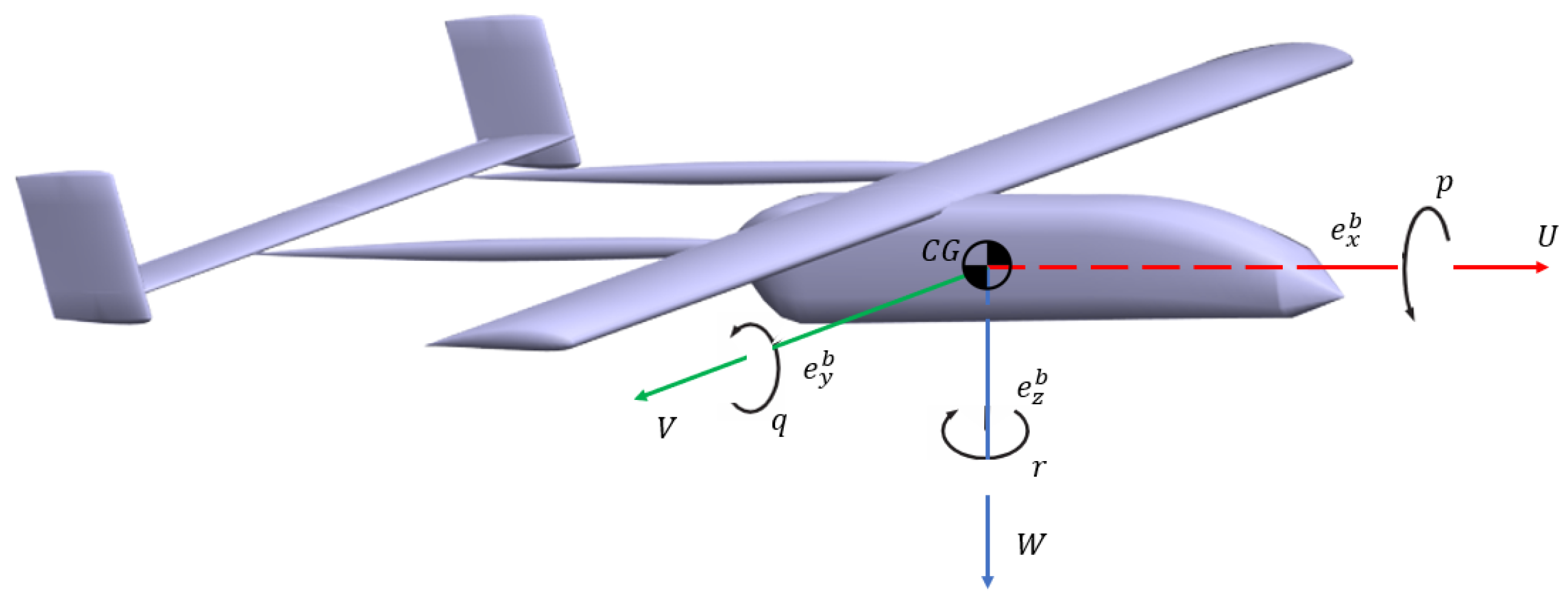
2. Flight Dynamics Model

The dynamics equations that will be briefly discussed in this section represent the dynamic equilibrium of translation and rotation around the aircraft’s center of gravity, with respect to the inertial frame ${\mathcal{F}}^{\mathcal{I}}$. Such an approach will lead to us attaining the dynamics of the aircraft by means of two vector equations (six scalar equations) [28,29].

We assume the kinematic quantities required to describe the rigid body motion of an aircraft, namely ${\mathit{v}}_{CG}$ describing the center of gravity ($CG$) position rate of change in ${\mathcal{F}}^{\mathcal{I}}$ and ${\mathit{\omega }}_{\mathcal{B}/\mathcal{I}}$ as the angular velocity of the body triad also referred to as ${\mathcal{F}}^{\mathcal{I}}$, collecting them within a single vector, yielding

$${\mathit{w}}_{CG}={\{{\mathit{v}}_{CG},{\mathit{\omega }}_{\mathcal{B}/\mathcal{I}}\}}^T.$$

(1)

The dynamic equilibrium can be expressed by means of the generalized balance equation:

(2)

where, in Equation (2), ${\mathit{M}}_{CG}$ represents the generalized inertia matrix encompassing the static moment tensor ${\mathit{S}}_{CG}$ and the inertia tensor ${\mathit{J}}_{CG}$ with respect to point $CG$, thus yielding

$${\mathit{M}}_{CG}=\left[\begin{array}{cc}m\mathbf{I}& {\mathit{S}}_{CG}^T\\ {\mathit{S}}_{CG}& {\mathit{J}}_{CG}\end{array}\right].$$

(3)

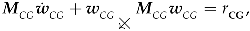
The term represents the generalized velocity vector with the southwest cross product operator applied. This operator rearranges the sub-vectors ${\mathit{v}}_{CG}$ and ${\mathit{\omega }}_{\mathcal{B}/\mathcal{I}}$ in a six-by-six matrix, filling it with their skew-symmetric forms, i.e., ${\mathit{v}}_{{CG}_{\times }}$ and ${\mathit{\omega }}_{{\mathcal{B}/\mathcal{I}}_{\times }}$, as the three-by-three antisymmetric matrices composed of their respective sub-vector components. More explicitly,

(4)

Newton’s principle, as expressed in Equation (2), representing an inertial reaction, can be represented in the scalar components in the body reference ${\mathcal{F}}^{\mathcal{B}}$. Considering the left-hand side of the equation, in particular ${\mathit{v}}_{CG}^{\mathcal{B}}={\left\{U,V,W\right\}}^T$ and ${\mathit{\omega }}_{\mathcal{B}/\mathcal{I}}^{\mathcal{B}}={\left\{p,q,r\right\}}^T$ as shown in Figure 1, according to the most common nomenclature adopted for aircraft dynamics [28,29], superscript ${\left(·\right)}^{\mathcal{B}}$ is employed to indicate the representation in the body reference ${\mathcal{F}}^{\mathcal{B}}$.

The right-hand side term ${\mathit{r}}_{\mathbf{CG}}$ in Equation (2) represents the generalized force term collecting together the aerodynamic, propulsive, and gravitational forces and moments, formally

$${\mathit{s}}_{CG}={\mathit{s}}_{CG}^a+{\mathit{s}}_{CG}^p+{\mathit{s}}_{CG}^g.$$

(5)

Each term in Equation (5) takes the form ${\mathit{s}}_{CG}^{\left(·\right)}={\left\{{\mathit{f}}^{\left(·\right)},{\mathit{m}}_{CG}^{\left(·\right)}\right\}}^T$, wherein ${\mathit{f}}^{\left(·\right)}$ is the force and ${\mathit{m}}_{CG}^{\left(·\right)}$ the moment with respect to the $CG$ position.

The management of the propulsive force term ${\mathit{s}}_{CG}^p$ has been meticulously devised to accurately represent propulsion-related forces and moments at designated measurement points. It includes factors such as the thruster number, responsiveness relative to the flight speed and air density, and spatial configuration. The expression for thruster forces and moments, made explicit by the components in the body reference ${\mathcal{F}}^{\mathcal{B}}$, is provided as follows:

$${\mathit{s}}_{CG}^{p^{\mathcal{B}}}={\mathit{s}}_{CG}^{p^{\mathcal{B}}}({\delta }_t,{\sigma }_i,{\gamma }_i,{\mathbf{r}}_{T_P}^{\mathcal{B}})=\sum _{i=1}^{N_t}{T}_i\left\{\begin{array}{cc}& \left\{\begin{array}{c}cos{\sigma }_{i}cos{\gamma }_i\\ sin{\sigma }_i\\ cos{\sigma }_{i}sin{\gamma }_i\end{array}\right\}\\ {\mathbf{r}}_{T_P}^{\mathcal{B}}\times & \left\{\begin{array}{c}cos{\sigma }_{i}cos{\gamma }_i\\ sin{\sigma }_i\\ cos{\sigma }_{i}sin{\gamma }_i\end{array}\right\}\end{array}\right\}.$$

(6)

Here, ${\mathbf{r}}_{T_P}$ represents the positional vector originating from the center of gravity $CG$ and extending towards the point of application of the thrust force $T_i$ exerted by the ith thruster. The angle ${\sigma }_i$ gauges the misalignment between the vertical plane of symmetry of the aircraft and the thrust line of the ith thruster. Similarly, ${\gamma }_i$ defines the angle between the projection of the ith thruster’s thrust line onto the vertical plane of symmetry and the $x^b$-axis. The thrust intensity $T_i$ is determined by the throttle setting ${\delta }_{t_i}$ as follows:

$$T_i=\widetilde{T_i}K\left({\delta }_{t_i}\right){\delta }_{t_i},$$

(7)

modulating the nominal thrust intensity $\widetilde{T_i}$ with a shaping function, $K\left({\delta }_{t_i}\right)$, to account for efficiency variations and nonlinear characteristics. The range of ${\delta }_{t_i}$ values can vary based on the thruster technology, allowing for features like reversal thrust forces in electric motors.

The gravity force term ${\mathit{s}}_{CG}^g$ is simply defined as a function of the mass m and aircraft attitude angles ${\mathit{e}}_{321}^{\mathcal{B}}={\{\phi ,\vartheta ,\psi \}}^T$, ordered according to a Tait–Bryan sequence [28,29]. The effect is described as a force acting in a downward direction at the center of gravity, yielding the corresponding analytic representation in the body reference ${\mathcal{F}}^{\mathcal{B}}$:

$${\mathit{s}}_{CG}^{g^{\mathcal{B}}}={\mathit{s}}_{CG}^{g^{\mathcal{B}}}(m,\phi ,\vartheta ,\psi )={\mathcal{R}}_{\mathcal{I}}^{{\mathcal{B}}^T}(\phi ,\vartheta ,\psi )\left\{\begin{array}{c}0\\ 0\\ mg\end{array}\right\}.$$

(8)

In Equation (8), the term ${\mathcal{R}}_{\mathcal{I}}^{\mathcal{B}}(\phi ,\vartheta ,\psi )$ represents the rotation from an inertial north–east–down reference [28,29] to a body reference as depicted in Figure 1, where g is the gravitational acceleration.

Finally, the aerodynamic force term ${\mathit{s}}_{CG}^a$ in Equation (5) is obtained through linear decomposition for the generalized state vector ${\mathit{w}}_{CG}^{\mathcal{B}}$ and the aerodynamic control vector ${\mathit{u}}^a$, which collects the elevator, aileron, and rudder deflection inputs together as

$${\mathit{u}}^a=\left\{\begin{array}{c}{\delta }_e\\ {\delta }_a\\ {\delta }_r\end{array}\right\}.$$

(9)

Thus, the general structure of this force term is made explicit in the body components by means of the matrices ${\mathcal{S}}_{CG}^{a^{\mathcal{B}}}$ and ${\mathcal{C}}_{CG}^{a^{\mathcal{B}}}$, namely the stability derivative and control sensitivity matrices, respectively, such that the current states and controls are proportionally weighted with their respective stability and control derivatives:

$$s_{CG}^{a^{\mathcal{B}}}=\left\{\begin{array}{c}X\\ Y\\ Z\\ \mathcal{L}\\ \mathcal{M}\\ \mathcal{N}\end{array}\right\}={\mathcal{S}}_{CG}^{a^{\mathcal{B}}}{\mathit{w}}_{CG}^{\mathcal{B}}+{\mathcal{C}}_{CG}^{a^{\mathcal{B}}}{\mathit{u}}^a.$$

(10)

In Equation (10), X, Y, and Z represent the usual components of the aerodynamic force in a body reference, and similarly $\mathcal{L}$, $\mathcal{M}$, and $\mathcal{N}$ are the components of the aerodynamic moment measured from the $CG$ position, expressed in the same body reference [28,29]. Complementing the dynamic model, a set of three nonlinear equations governs the attitude kinematics by expressing the rate of change of Euler’s angles as a function of the body angular rates [28]:

$${\dot{\mathit{e}}}_{321}={\mathbf{S}}_{321}^{{\mathcal{B}}^{-1}}{\mathit{\omega }}_{\mathcal{B}/\mathcal{I}}^{\mathcal{B}},$$

(11)

wherein ${\dot{\mathit{e}}}_{321}={\left\{\dot{\phi },\dot{\vartheta },\dot{\psi }\right\}}^T$.

To facilitate a dynamic simulation with the control logic proposed in the following, it is beneficial to present schematically a series of nonlinear first-order differential equations derived from the model just introduced:

(12)

The system of nine scalar differential equations in Equation (12) concisely describes the change in the aircraft state ${\mathit{x}}^{AC}={\left\{{\mathit{w}}_{CG}^{{\mathcal{B}}^T},{\mathit{e}}_{321}^T\right\}}^T$ over time, as a function of the current state and of the input array $\mathit{u}={\left\{{\mathit{u}}^{a^T},{\delta }_{T_i}\right\}}^T$, $i=1,\dots N_t$, where $N_t$ is the number of thrusters on board. Conceptually, Equation (12) stands for the aircraft dynamics block, which will be affected by the inputs computed using the control logic introduced in the following sections.

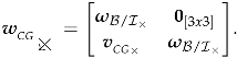
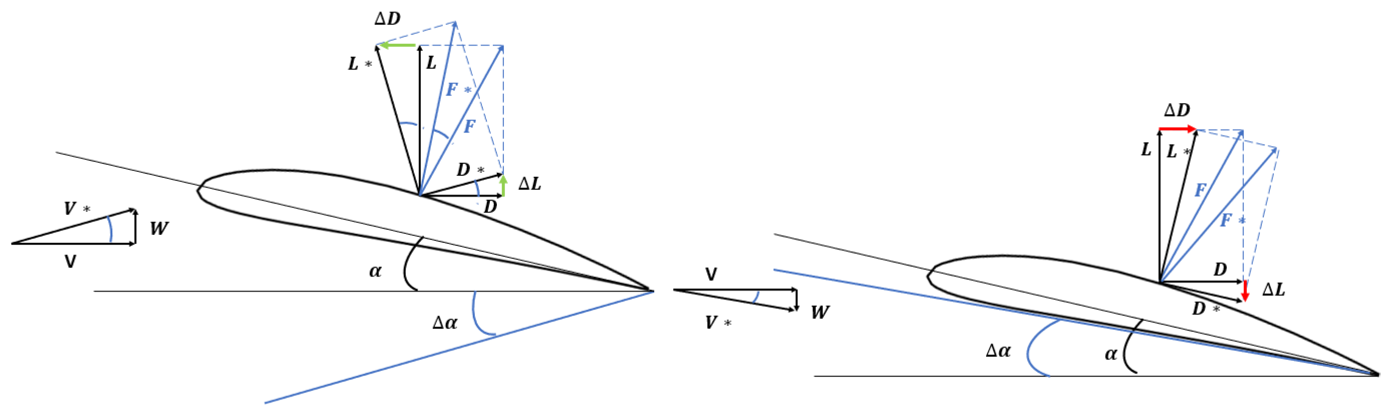
3. Aerodynamic Modeling

In the previous section, an effective dynamic modeling approach was addressed to accurately capture the nonlinear dynamics of the aircraft. At this level of complexity, the proposed aerodynamic modeling represents a commendable balance between computational resources and model fidelity. However, for our purposes, it is crucial to consider that the system to be simulated is not an isolated entity but a multi-agent system composed of units operating in coordination and in close proximity. Therefore, it was imperative to develop a model that accounts for the aerodynamic interactions among individual aircraft, capturing the effects of these interactions and the resulting modifications in the aerodynamic field for trailing aircraft. This field features an upwind region in the outer portion of the wake and a downwind region in the inner portion (see Figure 2). The induced velocity effect results in either a positive or negative change in the angle of attack of the trailing aircraft, depending on its sideward displacement relative to the leading one.

As shown in Figure 3, in the upwind region, the increase in the induced angle of attack causes the resultant aerodynamic forces to tilt forward. Consequently, the aircraft experiences an increase in lift, accompanied by a reduction in drag. Conversely, in the downwind region, the opposite effect occurs. The decreased angle of attack leads to a reduction in lift and an increase in drag, which results in generally higher fuel consumption and degraded flight performance [31,32].

An investigation in this regard was not only valuable for improving the accuracy of the dynamic model but also justified the selection of a specific formation geometry. The intent was to allow each aircraft to fly in what is commonly referred to as the “sweet spot”, which is the outer region near the wingtip of the leading aircraft [30]. This region enables the trailing aircraft to take advantage of the upwash region, resulting in reduced induced drag and, consequently, lower fuel consumption.

To investigate the wake effects, a mid-fidelity approach based on the vortex lattice method (VLM) was employed [33], with leading and trailing lifting surfaces. Although the VLM provides a simplified representation of flow physics, it is widely accepted and adopted for studying and analyzing aircraft aerodynamics in formation flight, featuring a favorable balance of accuracy and the computational cost for the task.

Formally, assuming a concentrated-parameter aerodynamic model [34], the wake contribution is counted as an additive $\Delta C$ component, which changes the aerodynamic behavior of the isolated aircraft as a function of the relative intra-swarm separation vector $\Delta \mathit{s}$ encompassing its three longitudinal ($\Delta x$), lateral ($\Delta y$), and vertical ($\Delta z$) components relative to the preceding aircraft forming the wake, such that $\Delta \mathit{s}={\left\{\Delta x,\Delta y,\Delta z\right\}}^T$. Correspondingly, the analytic description of the generic aerodynamic coefficient for a follower aircraft can be given as

$$C_i\left(\dots ,\Delta \mathit{s}\right)=C_{i_0}+C_{i_{\alpha }}\alpha +C_{i_{\widehat{\dot{\alpha }}}}\widehat{\dot{\alpha }}+C_{i_{\widehat{q}}}\widehat{q}+C_{i_{{\delta }_e}}{\delta }_e+\Delta C_i(\Delta \mathit{s})$$

(13)

for longitudinal aerodynamics and

$$C_j\left(\dots ,\Delta \mathit{s}\right)=C_{j_0}+C_{j_{\beta }}\beta +C_{j_{\widehat{\dot{\beta }}}}\widehat{\dot{\beta }}+C_{j_{\widehat{p}}}\widehat{p}+C_{j_{\widehat{r}}}\widehat{r}+C_{j_{{\delta }_a}}{\delta }_a+C_{j_{{\delta }_r}}{\delta }_r+\Delta C_j(\Delta \mathit{s})$$

(14)

for lateral–directional aerodynamics. In Equation (13), $\alpha$, $\widehat{\dot{\alpha }}$, and $\widehat{q}$ represent, respectively, the angle of attack of the aircraft, its non-dimensional rate, and the non-dimensional component of the angular rate around the pitch axis. In Equation (14), $\beta$, $\widehat{\dot{\beta }}$, $\widehat{p}$, and $\widehat{r}$ represent, respectively, the sideslip angle, its non-dimensional rate, and the two non-dimensional components of the angular rate around the roll and yaw axes.

4. Formation Guidance and Coordination in Different Mission Phases

A swarm of fixed-wing aircraft is a formation composed of several units. According to the formation governance paradigm assumed herein, each unit within the formation is designed to be equipped with an Autonomous Flight Control System (AFCS), removing the need for ground station control. Within the AFCS, two aircraft management modes coexist: the guidance mode (GM) and the Formation Control Mode (FCM). The GM will be dealt with in detail in Section 4.1, whereas the FCM will be presented in Section 4.2. The management of and interconnection between these two modes will be addressed in Section 4.3 and extensively through the results in Section 5. For now, it can be observed that the GM logic can be employed by each unit, depending on the mission phase and on the role of that unit in such a mission phase, which may be either a leader or follower.

4.1. Guidance Mode (GM)

Specifically, three guidance algorithms are investigated here, implemented in the GM of the AFCS to be employed in different legs of the flight:

• Beam tracking navigation. Employed during the cruise phase or linear ground reconnaissance. Described in Section 4.1.1 and Section 4.1.2.
• Circular trajectory tracking. Availed of during loitering or orbital reconnaissance around a fixed target. Described in Section 4.1.3.
• Rendezvous guidance. Implementing a specific control to reduce the space and time required for in-flight formation assembly. Described in Section 4.1.4.

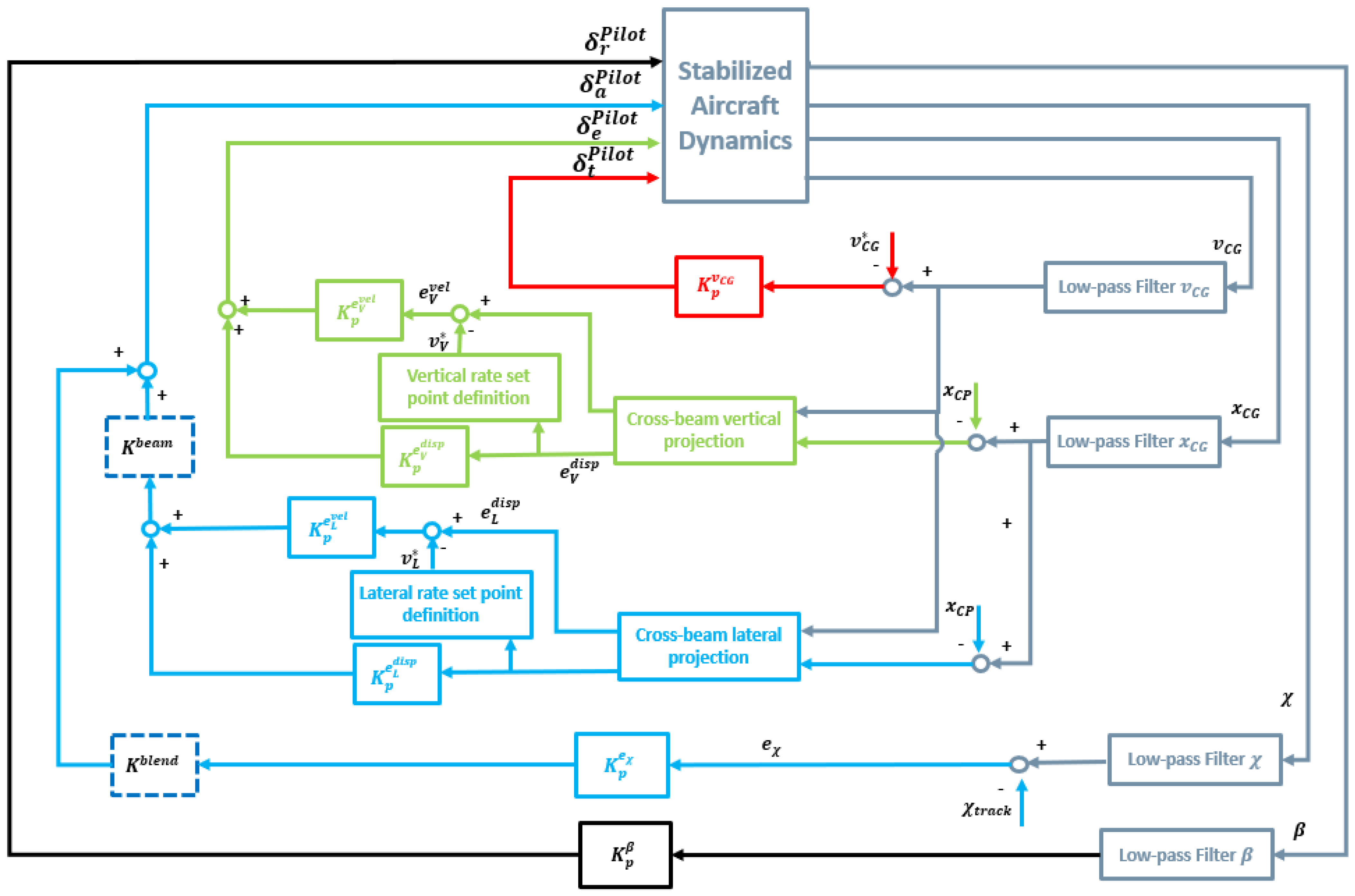
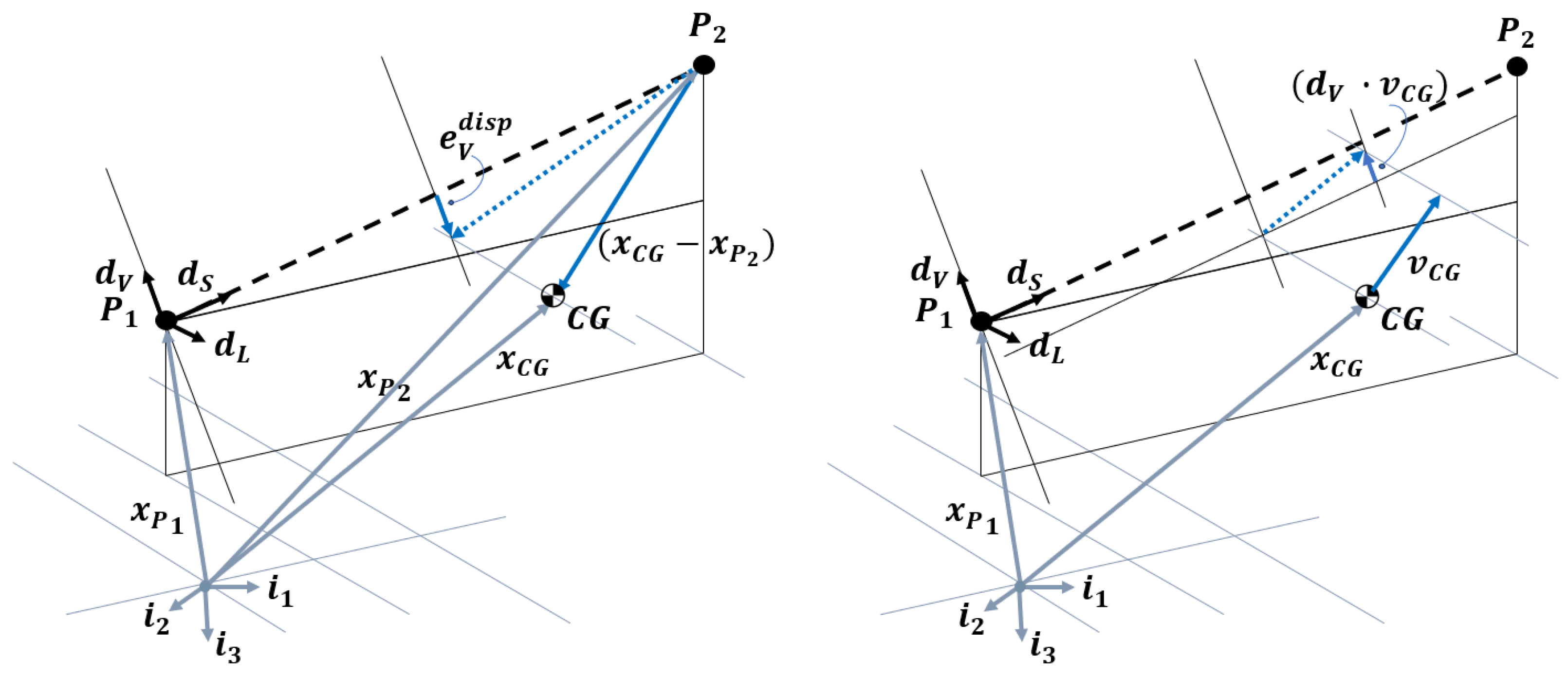
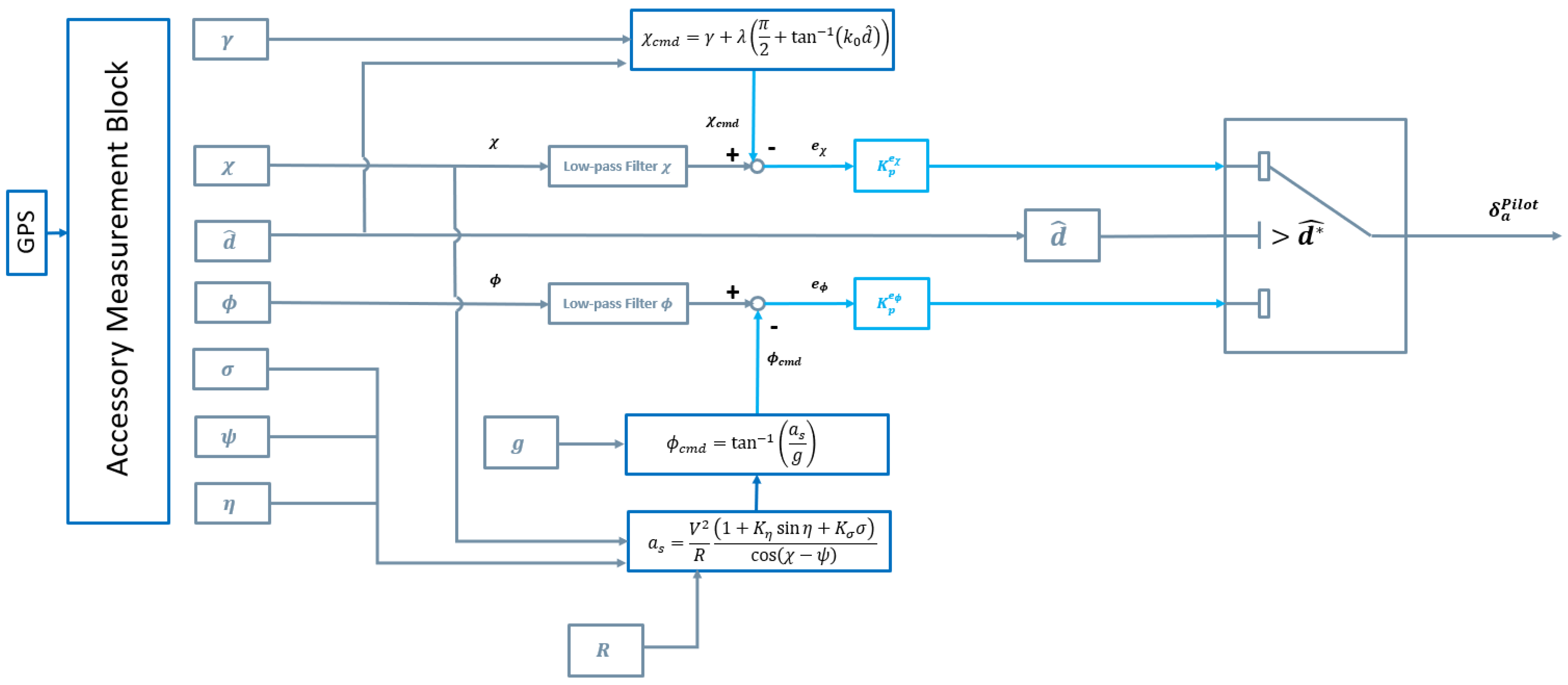
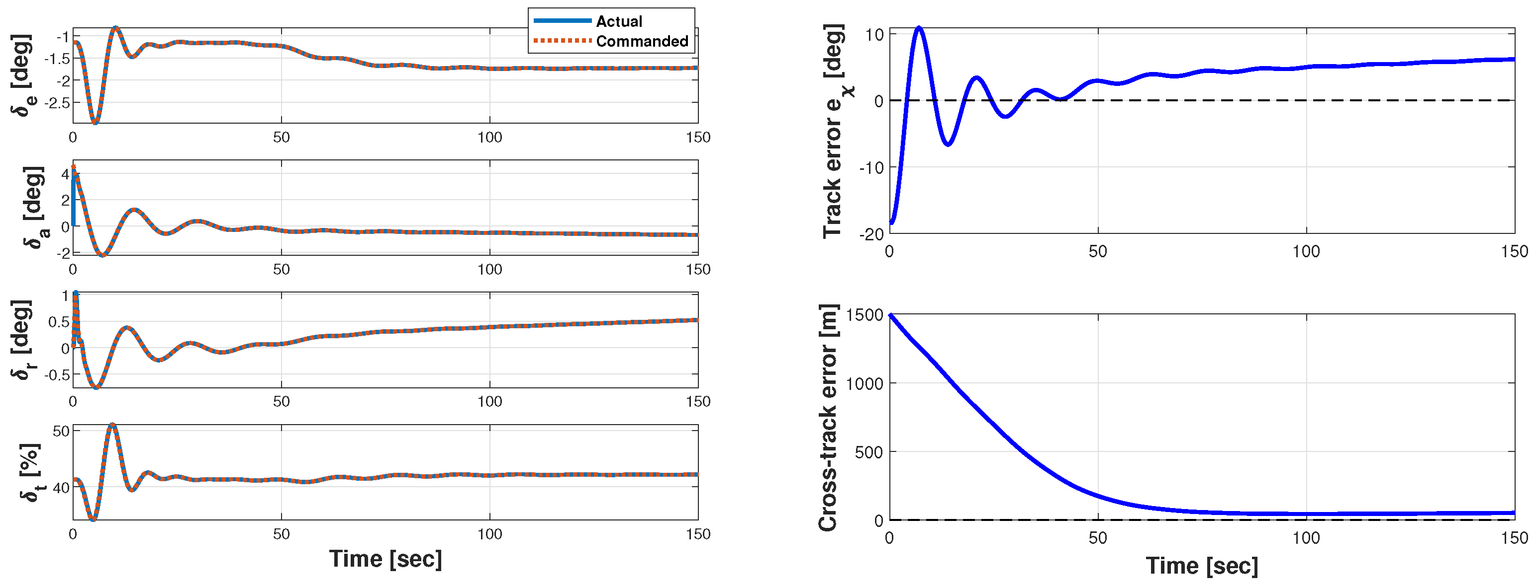
4.1.1. Beam Tracking

Following a pre-assigned set of checkpoints in three-dimensional (3D) space, connected by straight legs, is the problem at hand, which is essentially a means to achieve waypoint navigation. The purposeful guidance algorithm was inspired by prior original work carried out on airship guidance [35,36], in turn worked out from more standard control algorithms introduced for aircraft [37,38]. It essentially relies upon beam-tracking logic for both longitudinal and lateral–directional guidance, similar to that used for VOR navigation or ILS systems. This approach encompasses self-contained motion control along longitudinal and horizontal beam planes, defined contingent upon the orientation. A comprehensive scheme of the proposed beam-tracking control logic is reported in Figure 4. This will also be detailed in the next paragraph (Section 4.1.2), dealing with beam tracking and trajectory blending.

This is achieved by introducing a coordinate system fixed on the beam, composed of mutually orthogonal unit vectors centered at the departure checkpoint. The coordinate system is defined such that the unit vector ${\mathit{d}}_{\mathit{S}}$ aligns with the beam and is directed towards the destination checkpoint, the unit vector ${\mathit{d}}_{\mathit{V}}$ is orthogonal to ${\mathit{d}}_{\mathit{S}}$ pointing positively upwards, and ${\mathit{d}}_{\mathit{L}}$ completes the triad, indicating the rightward direction from above.

A formal definition of the beam-fixed triad with respect to the inertial frame ${\mathcal{F}}^{\mathcal{I}}$ is provided herein:

$$\begin{array}{cc}\hfill {\mathit{d}}_{\mathit{S}}& ={\displaystyle \frac{{\mathit{x}}_{P_2}-{\mathit{x}}_{P_1}}{\parallel {\mathit{x}}_{P_2}-{\mathit{x}}_{P_1}\parallel }},\hfill \\ \hfill {\mathit{d}}_{\mathit{H}}& ={\mathit{d}}_{\mathit{S}}·cos{\theta }_B,\hfill \\ \hfill {\mathit{d}}_{\mathit{L}}& ={\mathit{i}}_{\mathbf{3}}\times {\mathit{d}}_{\mathit{H}},\hfill \\ \hfill {\mathit{d}}_{\mathit{V}}& ={\mathit{d}}_{\mathit{L}}\times {\mathit{d}}_{\mathit{S}},\hfill \end{array}$$

(15)

where ${\mathit{x}}_{P_1}$ and ${\mathit{x}}_{P_2}$ represent the departure and destination checkpoints’ coordinates, respectively, from the origin of ${\mathcal{F}}^{\mathcal{I}}$, and ${\mathit{d}}_{\mathit{H}}$ is the projection of ${\mathit{d}}_{\mathit{S}}$ on the ${\mathcal{F}}^{\mathcal{I}}$ horizontal plane through the cosine of the beam elevation angle ${\theta }_B$.

The core strategy, based on the available GPS measurements, is a proportional control logic that aims to minimize the differences between the actual and desired ground speeds as well as address vertical and lateral positioning errors with respect to the intended path. Due to the aforementioned distinction between longitudinal and horizontal aircraft motion control, the two control laws will be presented individually, one at a time.

Longitudinal beam tracking. Longitudinal guidance is provided through the simultaneous employment of the throttle and elevator. A primary loop is closed on the aircraft’s ground speed magnitude $|{\mathit{v}}_{\mathit{CG}}|$ by adjusting the thrust setting through a proportional control law which aims to reduce the offset from a predefined set point, ${\mathit{v}}_{\mathit{CG}}^{\ast }$. Introducing the error $e_S=\left|{\mathit{v}}_{\mathit{CG}}\right|-{\mathit{v}}_{\mathit{CG}}^{\ast }$, the autothrottle control law is written as

$${\delta }_t^{Pilot}=k_p^{e_s}{e}_s,$$

(16)

where $k_p^{e_s}<0$ is selected to amplify the thrust setting when the aircraft ground speed falls below the desired set point ($e_s<0$) and, conversely, to reduce it when exceeding the target velocity ($e_s>0$).

Elevator control is employed for precise longitudinal position tracking by relying on two feedback variables: the vertical displacement error $e_V^{disp}$ and vertical velocity error $e_V^{vel}$. Indeed, as suggested by [37], it would be impractical to solely rely on position error control. Such an approach would result in a highly reactive control action as the aircraft would lack information on the direction of motion, leading to significant control inputs even for small position errors. Therefore, the distance between the aircraft’s $CG$ and the beam is computed in the vertical plane that contains the beam.

Geometrically, this can be expressed using the unit vector ${\mathit{d}}_{\mathit{V}}$ as shown in Figure 5. The unit vector ${\mathit{d}}_{\mathit{V}}$, as mentioned before, is defined as being normal to the straight line extending from $P_1$ to $P_2$ and lies within the vertical plane where the target beam is located. The formal expression for $e_V^{disp}$ is therefore

$$e_V^{disp}={\mathit{d}}_{\mathit{V}}·\left({\mathit{x}}_{CG}-{\mathit{x}}_{P_2}\right).$$

(17)

The vertical velocity error $e_V^{vel}$ is then computed as the difference between the measured projection of the aircraft inertial velocity vector ${\mathit{v}}_{\mathit{CG}}$ on ${\mathit{d}}_{\mathit{V}}$ and a target cross-beam vertical speed, $v_V^{\ast }$, obtained as a bounded linear function of the cross-beam displacement error $e_V^{disp}$ previously defined, written as

$$v_V^{\ast }\left(e_V^{disp}\right)=\left\{\begin{array}{cc}{v}_V^{\ast ,top},\hfill & \mathrm{if}{e}_V^{disp}<e_V^{disp,bot}\hfill \\ {\displaystyle \frac{e_V^{disp}}{e_V^{disp,bot}}}·v_V^{\ast ,top},\hfill & \mathrm{if}{e}_V^{disp,bot}\le e_V^{disp}\le 0\hfill \\ {\displaystyle \frac{e_V^{disp}}{e_V^{disp,top}}}·v_V^{\ast ,bot},\hfill & \mathrm{if}0\le e_V^{disp}\le e_V^{disp,top}\hfill \\ v_V^{\ast ,bot},\hfill & \mathrm{if}{e}_V^{disp}\ge e_V^{disp,top}\hfill \end{array}\right.$$

(18)

The boundary parameters involved in defining the cross-beam speed can be adjusted as control gains. Specifically, a positive velocity, $v_V^{\ast ,top}$, aligned with the ${\mathit{d}}_{\mathit{V}}$ direction, is commanded by the algorithm when reaching the maximum lower deviation limit of the beam, namely $e_V^{disp,bot}$. Conversely, a negative velocity, $v_V^{\ast ,bot}$, is commanded upon reaching the upper deviation limit $e_V^{disp,top}$. Finally, a percentage of $v_V^{\ast ,top}$ and $v_V^{\ast ,bot}$ is assigned proportionally to the deviation in cases where the positional error falls within the specified limits. At this juncture, the error $e_V^{vel}$ can be formally defined as

$$e_V^{vel}={\mathit{d}}_{\mathit{V}}·{\mathit{v}}_{\mathit{CG}}-v_V^{\ast }\left(e_V^{disp}\right).$$

(19)

In order to intuitively capture the measurement of the ${\mathit{d}}_{\mathit{V}}·{\mathit{v}}_{\mathit{CG}}$ term, a geometric sketch is provided in the right plot of Figure 5.

Building upon these feedback errors, the longitudinal beam-tracking control law for the elevator is assigned as

$${\delta }_e^{Pilot}=k_p^{e_v^{disp}}{e}_v^{disp}+k_p^{e_v^{vel}}{e}_v^{vel},$$

(20)

with $k_p^{e_v^{disp}}$ and $k_p^{e_v^{vel}}$ to be tuned such that the controller is configured to issue a negative ${\delta }_e^{Pilot}$ input inducing an upward trajectory curvature when the aircraft is positioned below the beam. Conversely, when the aircraft is positioned above it, the control input is set to a positive ${\delta }_e^{Pilot}$, determining a trajectory that steers the aircraft down towards the beam. The control action is modulated with the fine adjustment of the cross-beam speed in order to approach the correct positioning avoiding abrupt pull-up and push-over maneuvers.

Lateral–directional beam tracking. Horizontal guidance is achieved through two cooperative control loops: the first is dedicated to turn coordination, while the second is responsible for actual beam tracking.

Regarding turn coordination, a proportional control law is implemented to generate a rudder deflection that aims to minimize the sideslip angle and bring it closer to zero. Expressed analytically, the corresponding control law is

$${\delta }_r^{Pilot}=k_p^{\beta }\beta .$$

(21)

Conceptually, lateral beam tracking is executed in a manner similar to longitudinal beam tracking. In this case as well, the control action, assigned to the ailerons, is built upon a displacement error, defined as

$$e_L^{disp}={\mathit{d}}_{\mathit{L}}·\left({\mathit{x}}_{CG}-{\mathit{x}}_{P_2}\right),$$

(22)

which represents the projection of the distance of $CG$ from the destination checkpoint $P_2$, in the direction encoded by the unit vector ${\mathit{d}}_{\mathit{L}}$. The lateral cross-beam speed error is then measured as the difference between the projection of the $CG$ velocity on ${\mathit{d}}_{\mathit{L}}$ and a lateral rate set point, $v_L^{\ast }$, defined as a bounded linear function of $e_L^{disp}$:

$$v_L^{\ast }\left(e_L^{disp}\right)=\left\{\begin{array}{cc}{v}_L^{\ast ,top},\hfill & \mathrm{if}{e}_L^{disp}<e_L^{disp,bot}\hfill \\ {\displaystyle \frac{e_L^{disp}}{e_L^{disp,bot}}}·v_L^{\ast ,top},\hfill & \mathrm{if}{e}_L^{disp,bot}\le e_L^{disp}\le 0\hfill \\ {\displaystyle \frac{e_L^{disp}}{e_L^{disp,top}}}·v_L^{\ast ,bot},\hfill & \mathrm{if}0\le e_L^{disp}\le e_L^{disp,top}\hfill \\ v_L^{\ast ,bot},\hfill & \mathrm{if}{e}_L^{disp}\ge e_L^{disp,top}\hfill \end{array}\right.$$

(23)

with the tunable design parameters $v_L^{\ast ,top},v_L^{\ast ,bot},e_L^{disp,top}$, and $e_L^{disp,bot}$, such that a positive $e_L^{disp}$ arises from flying to the right side of the beam, thus prompting a negative $v_L^{\ast }$ adjustment when the maximum deviation $e_L^{disp,top}$ is exceeded, steering the aircraft toward the intended trajectory. Conversely, for a negative $e_L^{disp}$, the opposite scenario unfolds. A schematic of the beam-tracking measurements for lateral guidance is provided in Figure 6.

The analytic expression for $e_L^{vel}$ is then

$$e_L^{vel}={\mathit{d}}_{\mathit{L}}·{\mathit{v}}_{\mathit{CG}}-v_L^{\ast }\left(e_L^{disp}\right).$$

(24)

The control law for lateral beam tracking is finally derived by merging the two aforementioned feedback errors, resulting in the expression

$${\delta }_a^{Pilot}=k_p^{e_L^{disp}}{e}_L^{disp}+k_p^{e_L^{vel}}{e}_L^{vel}.$$

(25)

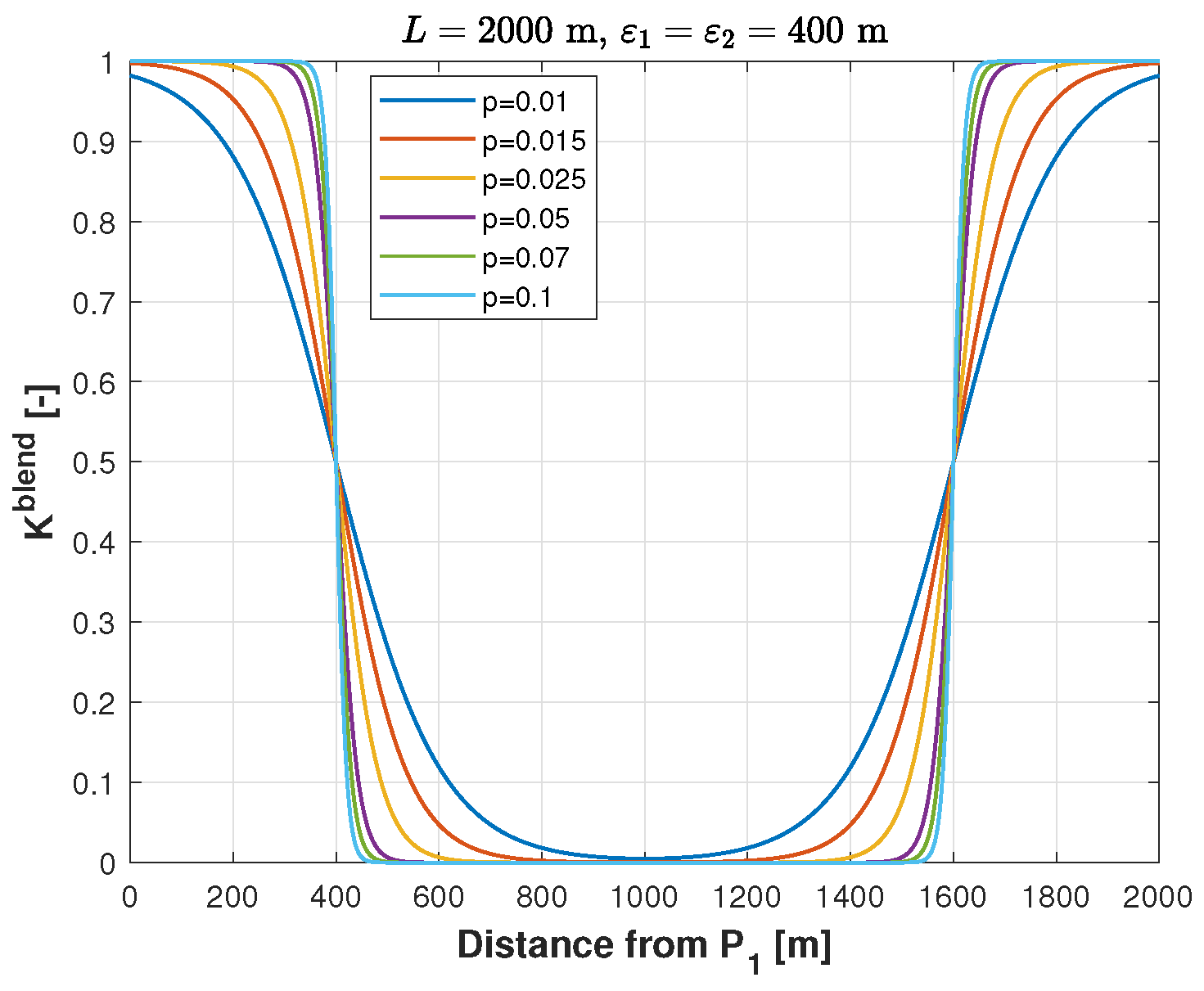
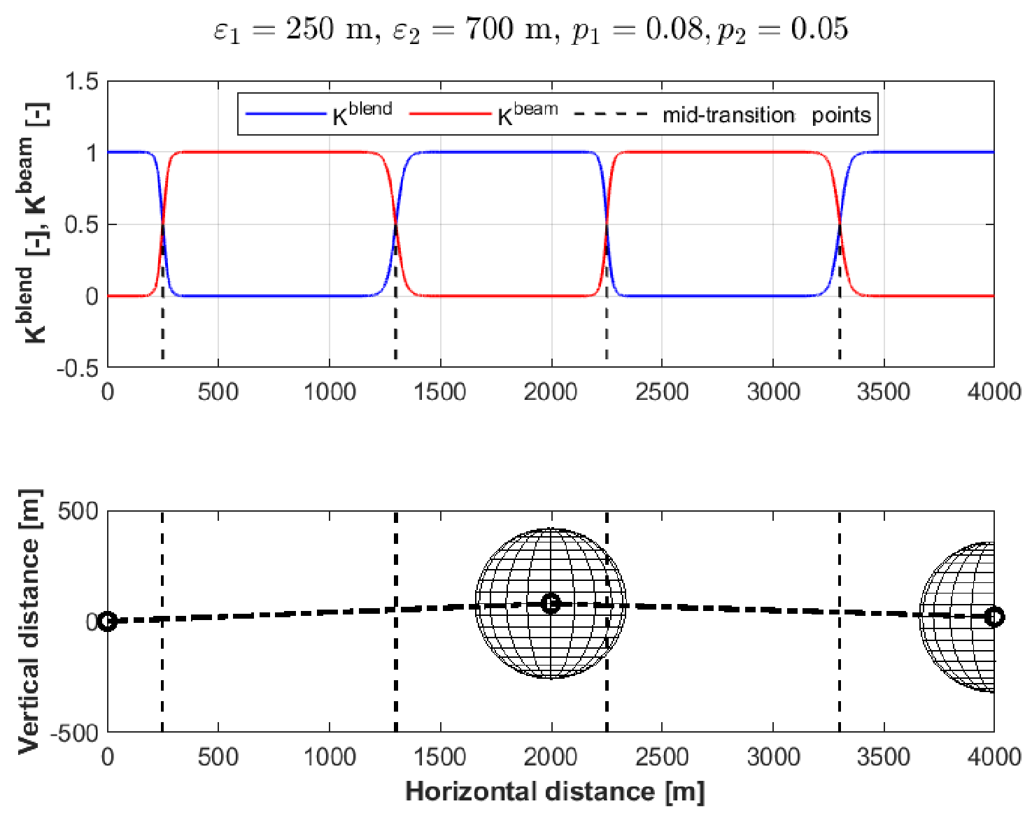
4.1.2. Trajectory Blending

During navigation, the aircraft might be assigned a route involving multiple changes in direction, which in turn require sharp course alterations between successive legs. Engaging the realignment maneuver only after crossing the current waypoint would certainly result in a trajectory overshoot that, at cruising speed, would take the aircraft significantly (i.e., potentially several hundred meters) out of position. To address this issue, an additional variable is incorporated into the controller design, namely, the radius $R_p$ of a proximity sphere centered at the waypoint. When the aircraft reaches a position within the spatial confines delineated by the proximity sphere, determined through GPS coordinate comparison, the control system triggers the realignment maneuver, guiding the aircraft toward the subsequent waypoint.

The method presented thus far for position control within the context of lateral beam tracking, however, loses effectiveness during abrupt course changes, dictated by the corresponding angolosity in the prescribed navigation path. This is due to the fact that in this case, as soon as the aircraft entered the proximity sphere, the control system would instantaneously register a significant lateral position error. Additionally, it would set the maximum lateral rate value to point the aircraft toward the new leg. The combination of these two errors would result in a sharp alteration of the control input, which could lead to unintended oscillations around the target leg or even cause the control input to become saturated.

One potential approach for mitigating this effect could involve reducing the gains $k_p^{e_L^{disp}}$ and $k_p^{e_L^{vel}}$ within the control law in Equation (25). However, this solution might lead to a decrease in the effectiveness of the control system in minimizing lateral position and velocity errors with respect to designated set points. In response, an exploration was conducted to integrate an additional control branch, specifically designed to facilitate trajectory blending.

Conceptually, this involves integrating a course error, such that the control system, by means of a specific proportional gain, $k_p^{e_{\chi }}$, aims to minimize the offset between the actual track angle ${\chi }^{A/C}$ (which corresponds to the horizontal azimuth heading $\psi$ in still air) and the designated ground course ${\chi }^{track}$. The analytic definition of such an error is correspondingly

$$e_{\chi }={\chi }^{A/C}-{\chi }^{track}.$$

(26)

The exclusive use of this error as the only feedback variable for lateral guidance (i.e., at the level of Equation (25)), however, proves ineffective. This is because, in order to ensure precise path tracking and a rapid response to any disturbances, it is necessary to maintain a fairly high value for $k_p^{e_{\chi }}$, especially compared to $k_p^{e_L^{disp}}$ and $k_p^{e_L^{vel}}$ (higher by several orders of magnitude). This approach leads to a situation where, during a change of course along the route, the aircraft quickly aligns itself with the designated course, yet retains a residual position offset, with respect to the target leg, that remains uncompensated.

To harness both control logic strategies, a concept was conceived to combine them using two variable gains, namely $K^{blend}$ and $K^{beam}$ (one being the reciprocal of the other), as a function of the distance traveled from the departure checkpoint. Indeed, it is crucial to underline that every leg is handled as a separate course. Consequently, the destination checkpoint of the current leg transitions into the departure checkpoint for the succeeding leg as soon as the aircraft enters the proximity sphere. This strategy entrusts lateral guidance solely to the course error during maneuvering phases and realignment with the subsequent leg. Meanwhile, once alignment is attained, the control system operates based solely on the position and velocity errors, facilitating precise beam tracking and swift disturbance rejection.

A candidate function suitable for this purpose could be a sigmoid function, which guarantees a smooth transition of the gain $K^{blend}$ from 0 to 1 as the aircraft approaches the destination checkpoint shortly before initiating the realignment maneuver. Subsequently, it transitions from 1 to 0 at the outset of the next leg to provide seamless maneuver continuity prior to the activation of the beam-tracking control. The analytic expression for the sigmoid function is

$$K^{blend}\left({\tilde{d}}_{P_1}\right)={\displaystyle \frac{1}{\left(1+e^{-p_2\left({\tilde{d}}_{P_1}-L+{\epsilon }_2\right)}\right)}}+\left(1-{\displaystyle \frac{1}{\left(1+e^{-p_1\left({\tilde{d}}_{P_1}-{\epsilon }_1\right)}\right)}}\right),$$

(27)

where ${\tilde{d}}_{P_1}=\parallel {\mathit{x}}_{CG}-{\mathit{x}}_{P_1}\parallel$ represents the distance covered from the departure checkpoint, L denotes the length of the current leg, and the parameters $p_1$ and $p_2$ are used to regulate the gain transition rate from 1 to 0 (at the onset of the subsequent leg) and from 0 to 1 (shortly before the realignment maneuver initiation), respectively; ${\epsilon }_1$ and ${\epsilon }_2$ signify the distances from the starting checkpoint and the destination checkpoint, respectively, at which the transition is intended to achieve a value of 0.5 (mid-transition).

In Figure 7, the behavior of $K^{blend}$ is depicted for different values of parameter $p=p_1=p_2$, along with fixed values for the parameter ${\epsilon }_1={\epsilon }_2=$ 400 m. The leg length is $L=$ 2000 m in this example.

Consequently, the expression for $K^{beam}$ is written as

$$k^{beam}\left({\tilde{d}}_{P_1}\right)=\left(1-K^{blend}\left({\tilde{d}}_{P_1}\right)\right).$$

(28)

The lateral guidance control law in Equation (25) can be restated by including the supplementary control branch for trajectory blending:

$${\delta }_a^{Pilot}=K^{beam}\left({\tilde{d}}_{P_1}\right)\left(k_p^{e_L^{disp}}{e}_L^{disp}+k_p^{e_L^{vel}}{e}_L^{vel}\right)+K^{blend}\left({\tilde{d}}_{P_1}\right)k_p^{e_{\chi }}{e}_{\chi }.$$

(29)

The guidance system in Figure 4 is applied to the stabilized aircraft dynamics, on account of the fact that a Stability Augmentation System (SAS) can be applied to condition the free dynamics of the aircraft, specified by the model in Equation (12) [28,29]. The need for this additional inner layer is generally dictated by the intrinsic constructive features of the machine at hand. As is known, except for with extreme aerodynamic configurations or mass distributions on board, this type of control (when at all featured) is generally not aggressive, thus leaving a significant authority margin for further control layers to act. A brief discussion of a possible implementation of this controller will be featured in Section 5, with application to a specific testbed.

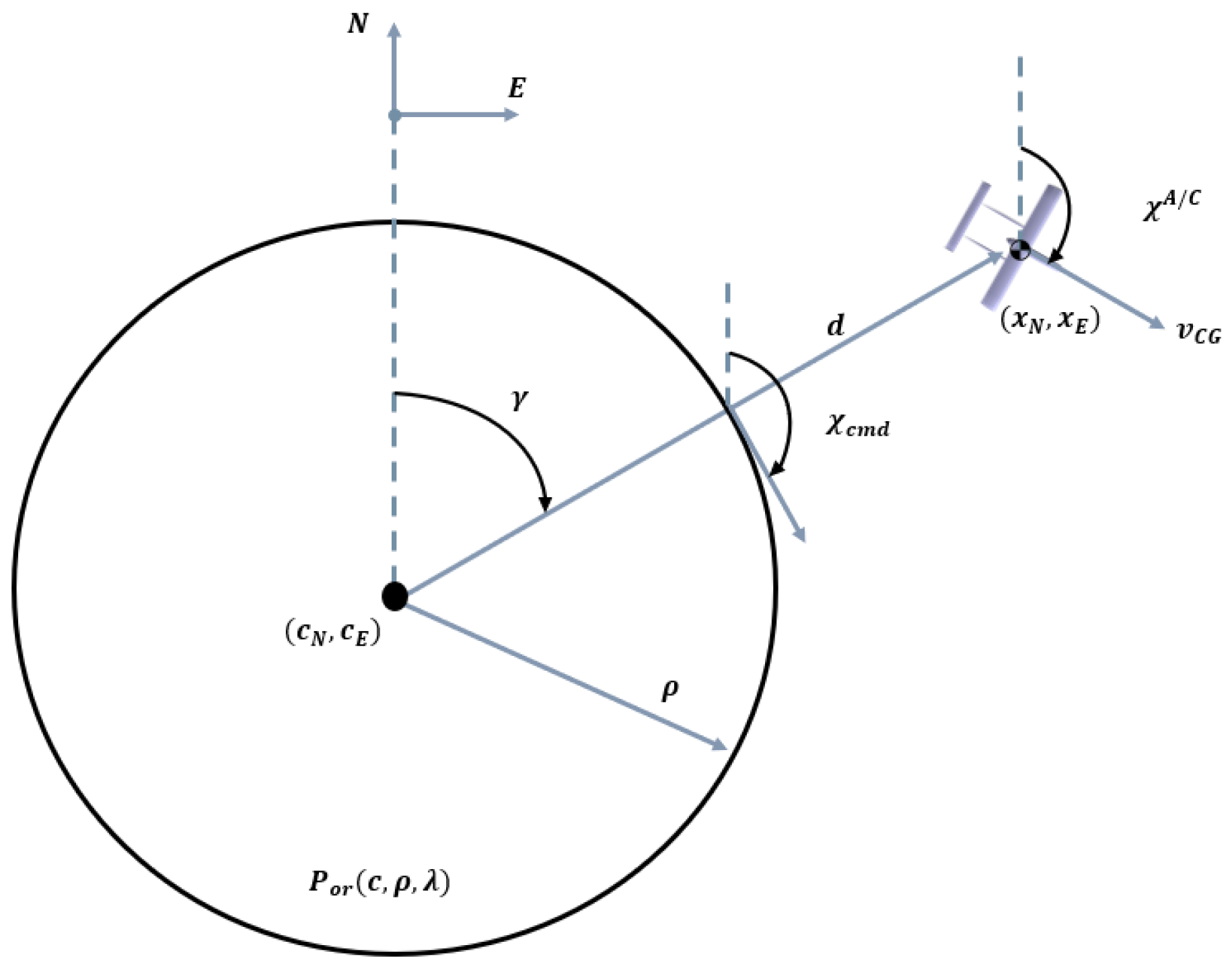
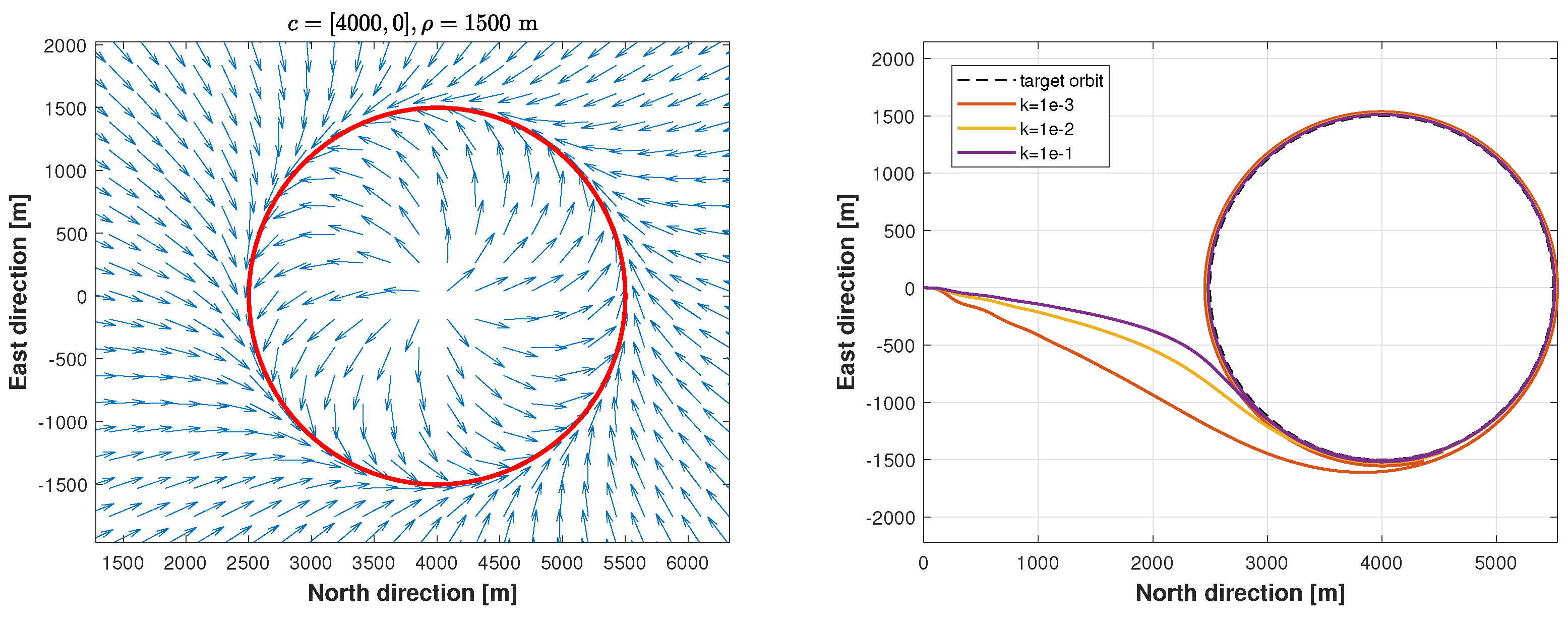
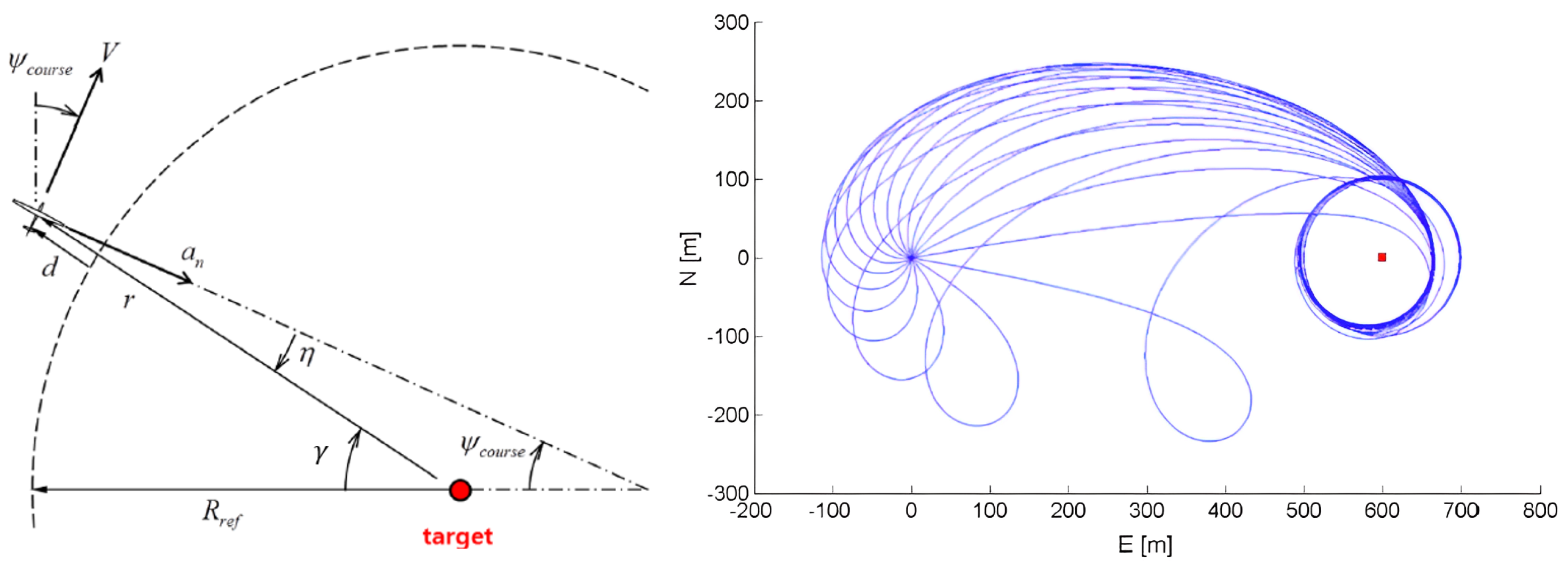
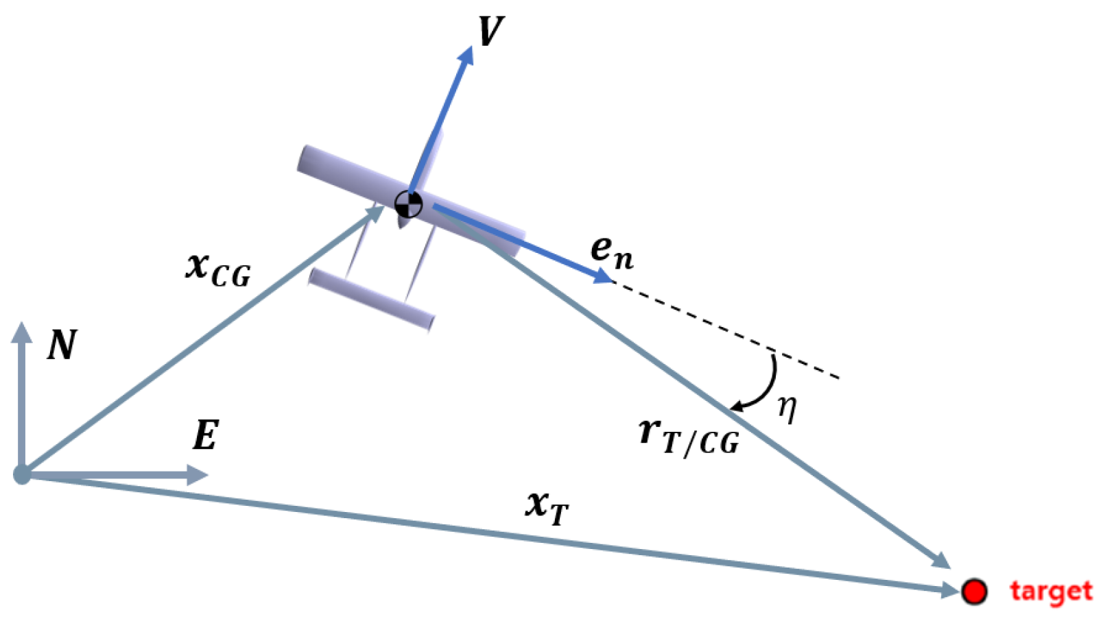
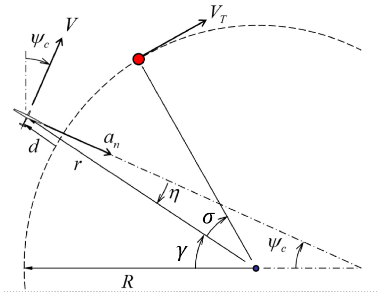
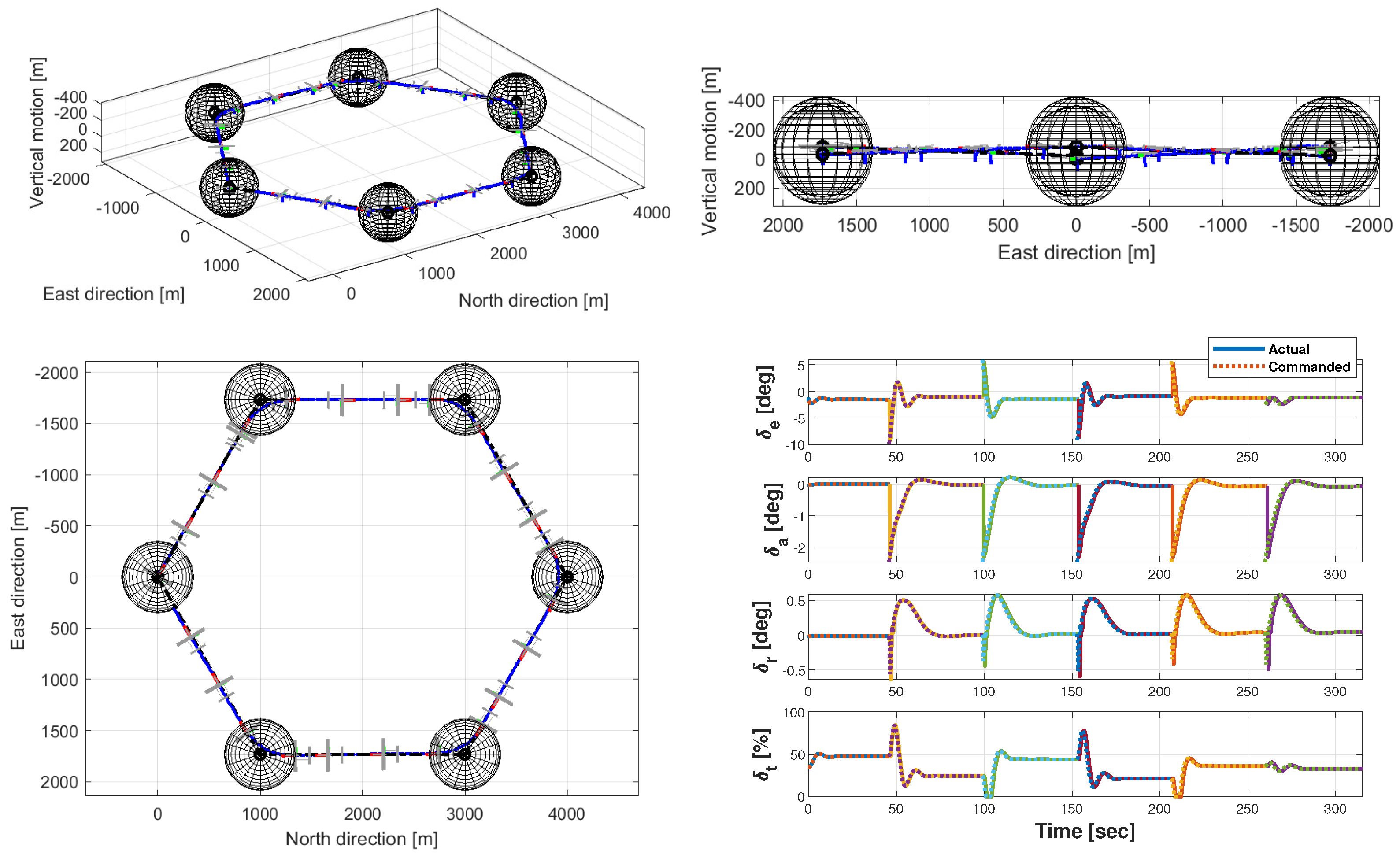
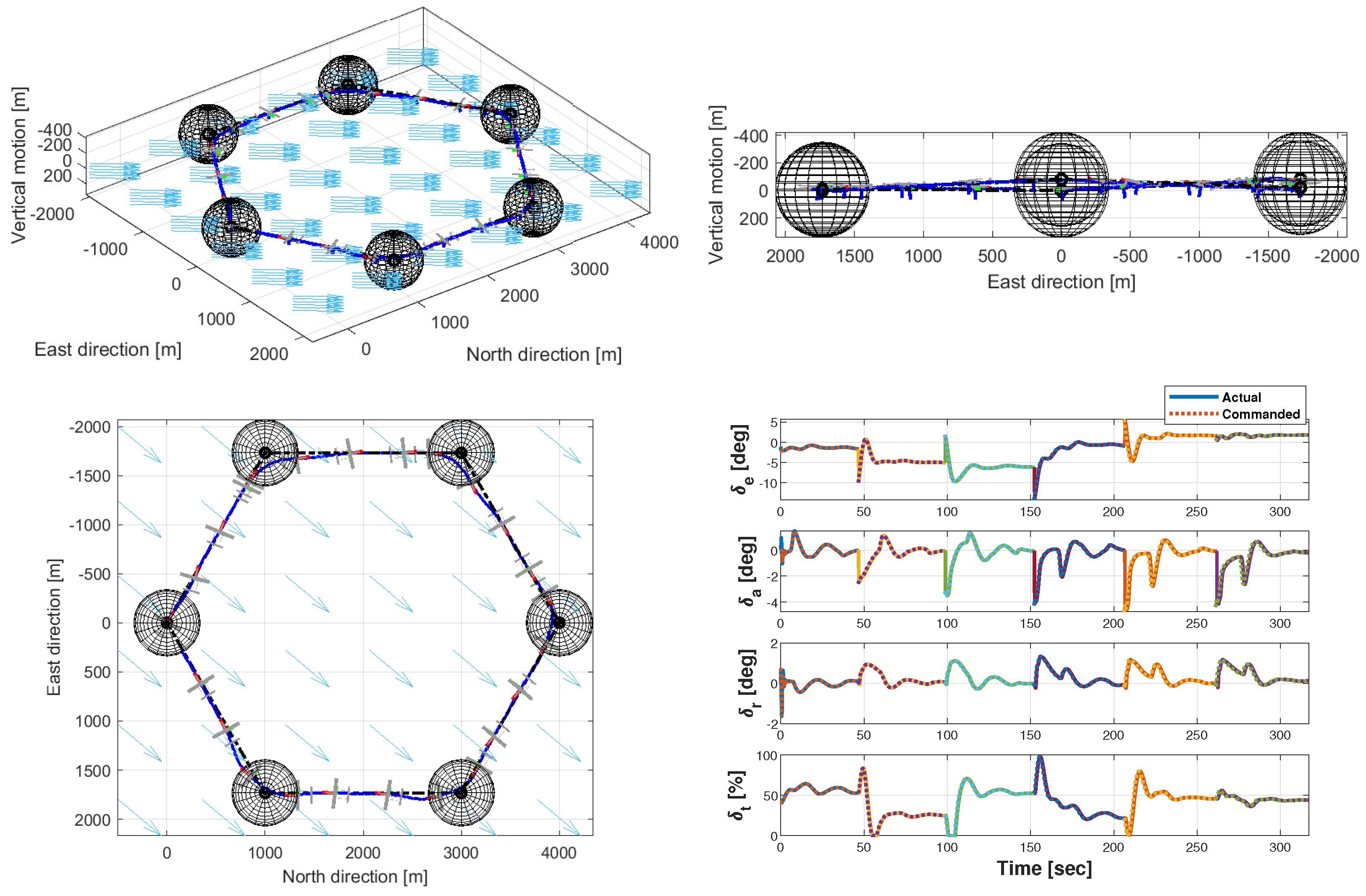
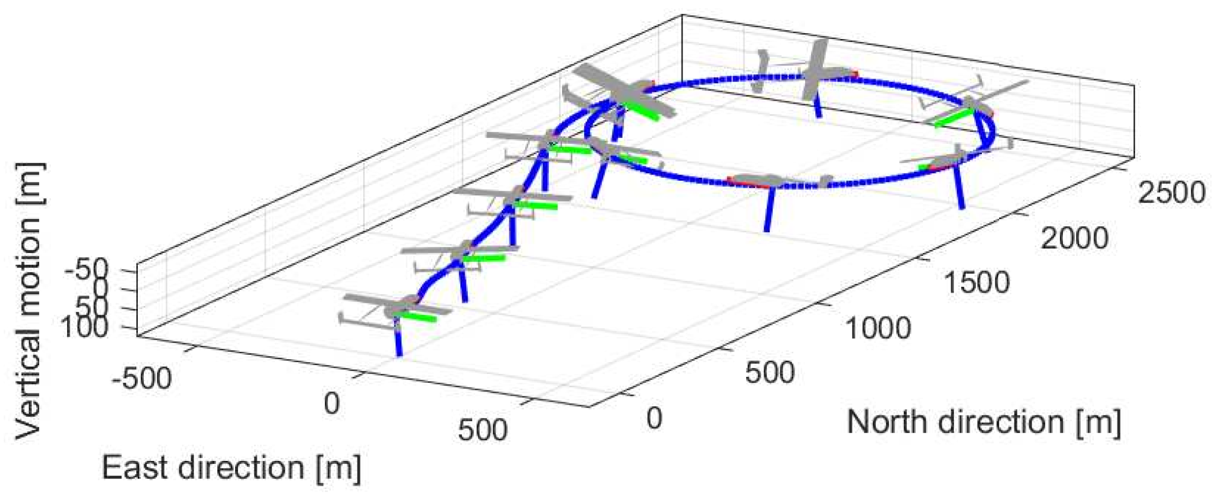
4.1.3. Circular Trajectory Tracking

For the execution of circular trajectories, inspiration was drawn from several previous works centered around the employment of a vector field-based guidance method [15,39]. In contrast to the earlier situation (see Section 4.1.1) wherein altitude alterations were attainable via beam tracking, the focus here lies on pursuing a circular trajectory entirely confined within the horizontal plane of the inertial frame, thus maintaining a constant altitude. Furthermore, it is possible to simplify the set of coordinates describing the inertial position of the aircraft, namely ${\mathit{x}}_{CG}={\left\{x_N,x_E\right\}}^T$, as the north and east position coordinates, respectively.

Essentially, the proposed approach aims to asymptotically bring the cross-track error to zero by means of the course error $e_{\chi }$ as the only feedback variable for lateral guidance. Consequently, regardless of the relative position of the UAV with respect to the required path, the commanded course angle ${\chi }_{cmd}$ must prompt the UAV to move toward the path itself. The ensemble of commanded course angles constitutes what is termed a vector field. This designation is apt as it represents an array of vectors comprising unit course vectors that indicate the desired travel direction.

Orbit path definition. Consider a generic orbit described by the following equation:

$${\mathbf{P}}_{or}(\mathbf{c},\rho ,\lambda )=\{\mathbf{r}\in {\mathbb{R}}^2:\mathbf{r}=\mathbf{c}+\lambda \rho {\left\{cos\gamma ,sin\gamma \right\}}^T,\gamma \in [0,2\pi )\},$$

(30)

where vector $\mathbf{c}$ represents the orbit center, whereas scalars $\rho$ and $\gamma$ stand for the radius and phase angle, respectively. An additional integer parameter, $\lambda \in [-1,+1]$, is introduced to define a counterclockwise or clockwise travel direction, respectively.

Upon designating the radius of the orbit and center coordinates (in the inertial reference frame) as $\mathbf{c}={\left\{c_N,c_E\right\}}^T$, it becomes feasible to ascertain the polar coordinate position of the aircraft relative to the orbit. Specifically, $d=\parallel {\mathit{x}}_{CG}-\mathbf{c}\parallel$ is the distance of the aircraft from the orbit center, and the phase angle is computed as

$$\gamma =arctan\left({\displaystyle \frac{x_E-c_E}{x_N-c_N}}\right).$$

(31)

Vector field generation. Let us define the cross-track error as the distance between the aircraft and the circumference of the orbit, which, in turn, is

$$\widehat{d}=d-\rho .$$

(32)

Now, it is beneficial to create a suitable function to determine the vector field of the unit course vectors based on the cross-track error. This function should operate in such a way that when the cross-track error $\widehat{d}$ is large, it guides the aircraft toward the center of the orbit. Conversely, when the aircraft approaches the perimeter of the orbit, the function should curve the trajectory by ${\displaystyle \frac{\pi }{2}}$ with respect to the current phase angle (Figure 8). This curvature will force the aircraft to follow the tangential direction to the orbit perimeter, according to the orbit travel direction ($\lambda$).

Therefore, it is possible to express the commanded course angle as

$${\chi }_{cmd}=\gamma +\lambda \left({\displaystyle \frac{\pi }{2}}+{tan}^{-1}\left(k_0\widehat{d}\right)\right),$$

(33)

with $k_0$ as a tunable parameter that regulates the transition rate to the orbit path.

The control structure remains basically consistent with that used for beam tracking (see Figure 4). Similarly, the existing control loops for airspeed tracking and turn coordination can be adopted in the same fashion. The control loop originally employed for longitudinal beam tracking can be adapted for altitude holding, by choosing checkpoints at the same altitude level. Lateral guidance is achieved by applying aileron deflections proportionate to the course error $e_{\chi }={\chi }^{A/C}-{\chi }_{cmd}$, by means of the same gain, $k_p^{e_{\chi }}$, used for trajectory blending:

$${{\delta }_a}^{Pilot}=k_p^{e_{\chi }}{e}_{\chi }.$$

(34)

An example of a vector field plot for circular trajectory tracking and the effect of the $k_0$ parameter on orbit transition rate adjustment are depicted, respectively, in the left and right plots in Figure 9. Specifically, a counterclockwise travel direction has been considered in this example.

4.1.4. Rendezvous Guidance

The rendezvous problem is now addressed to encompass the scenario of a real-world mission, considering the potential for swarm assembly during flight. This scenario contemplates an initial condition where multiple aircraft approach the rendezvous point from different directions.

There are two main possible techniques for achieving an in-flight rendezvous, which will be discussed shortly herein.

• Linear rendezvous. In the linear rendezvous technique, multiple aircraft converge on a common point along a straight line. This approach is characterized by its simplicity and is suitable for scenarios where vehicles need to assemble quickly. Among the basic advantages of this technique are its simplicity in planning and execution, as well as the ability to cater for an arbitrary number of components in the formation. Furthermore, this trajectory minimizes the travel distance. On the cons side, a straight trajectory is predictable and hence easy to intercept, and wind may hinder the rendezvous maneuver.
• Circular rendezvous. This technique involves aircraft converging on a central point along the circumference of a circle. The major advantages of this maneuver rest in the ease of constant communication with multiple neighbors and the chance to complete the assembly phase of the swarm within a relatively compact space, thus reducing the chance of encroaching into hostile territory or collisions due to orographic constraints. Conversely, on the cons side is the potentially longer time for completing the rendezvous maneuver compared to a straight-trajectory maneuver.

For a typical small-scale, low-powered UAV, optimized for range or endurance, the installed power limitations usually restrict the attainable range of velocities within the established flight envelope. This constraint may present challenges when contemplating a linear rendezvous scenario, particularly when the aircraft are approaching from considerable distances. Consequently, a preference emerges for the adoption of a circular rendezvous procedure. In this approach, a leader positions itself on a stable circular trajectory and awaits the incoming followers. The followers can perform simple coordination maneuvers to enter the circular path and chase the leader. Additionally, phasing techniques can be employed to expedite the process: these involve tightening the circular trajectory to reduce the phase angle separating the leader from the followers.

The procedure proposed herein is a fusion of two distinct guidance techniques: the first is based on circular trajectory tracking using the vector field approach discussed in Section 4.1.3. Incoming aircraft from various directions converge onto a stable circular trajectory. Subsequently, the phasing procedure introduced by [40] for leader chasing comes into play.

Circling over a fixed target. The proposed approach is an extension of that in [41], in which the gradual convergence of the aircraft around a fixed point, the center of the circular path, is ensured, regardless of the initial point and direction. This accomplishment is achieved by imposing an additional component of lateral acceleration beyond that needed for flying steadily on the circumference, proportional to the side-bearing angle $\eta$ (left plot in Figure 10), effectively steering the UAV along the intended circular trajectory.

This acceleration component can be written as

$$a_n={\displaystyle \frac{V^2}{R_{ref}}}(1+K_{\eta }sin\eta ).$$

(35)

A procedure for side-bearing angle computation using the GPS position and velocity is outlined here, referring to Figure 11.

We define the relative position ${\mathit{r}}_{\mathit{T}/\mathit{CG}}$ as the vector pointing from the aircraft’s $CG$ toward the orbit center (target): ${\mathit{r}}_{\mathit{T}/\mathit{CG}}={\mathit{x}}_{\mathit{T}}-{\mathit{x}}_{\mathit{CG}}={\{{r_{T/CG}}^N,{r_{T/CG}}^E\}}^T$. By labeling the inertial velocity components as ${\{V_N,V_E\}}^T$, the unit vector normal to the velocity direction is given by

$${\mathit{e}}_{\mathit{n}}={\displaystyle \frac{1}{V}}\left[\begin{array}{cc}0& -1\\ 1& 0\end{array}\right]\left\{\begin{array}{c}{V}_N\\ V_E\end{array}\right\},$$

(36)

where $V=\sqrt{V_N^2+V_E^2}$. Subsequently, applying the cross product property for the sine of the included angle between ${\mathit{e}}_{\mathit{n}}$ and ${\mathit{r}}_{\mathit{T}/\mathit{CG}}$ results in

$${\mathit{e}}_{\mathit{n}}\times {\mathit{r}}_{\mathit{T}/\mathit{CG}}=|{\mathit{e}}_{\mathit{n}}\left|\right|{\mathit{r}}_{\mathit{T}/\mathit{CG}}|sin\eta {\mathit{e}}_{\mathit{d}}=\left|{\mathit{r}}_{\mathit{T}/\mathit{CG}}\right|sin\eta {\mathit{e}}_{\mathit{d}}.$$

(37)

The equation is then solved for $sin\eta$:

$$sin\eta ={\displaystyle \frac{e_n^N·r_{\mathrm{T}/\mathrm{CG}}^E-e_n^E·r_{\mathrm{T}/\mathrm{CG}}^N}{\sqrt{{\left(r_{\mathrm{T}/\mathrm{CG}}^N\right)}^2+{\left(r_{\mathrm{T}/\mathrm{CG}}^E\right)}^2}}},$$

(38)

where in Equation (38), ${\left(·\right)}^N$ and ${\left(·\right)}^E$ represent the components in a northern or eastern direction, respectively. This guidance procedure, on its own, serves as an alternative to the previously discussed technique for circular trajectory tracking using the vector field method. However, the latter is favored because it ensures the circular path will be reached more swiftly, relying on a more direct and accessible measure over longer distances, which is the course angle $\chi$.

Once the leader has positioned itself within the rendezvous orbit, the followers, as they approach the perimeter, are guided by the phasing procedure specifically designed for leader chasing. At this stage, it is advantageous to rely on lateral acceleration as the control driver to generate small trajectory adjustments that lead the followers to assemble in the formation along the circular path.

Leader chasing. Motivated by the guidance law in Equation (35), a modification is made for the purpose of a rendezvous with a reference point (i.e., the designated leader) that moves along the circular path. Figure 12 shows the geometric scheme that will help to carry out the proposed guidance law. It is assumed that the follower’s airspeed is set to be equal to the leader’s airspeed, or analytically that $V=V_T$, where $V_T$ is the velocity of the leader.

The control system then applies normal acceleration, which is determined by the following expression:

$$a_n={\displaystyle \frac{V^2}{R_{ref}}}(1+K_{\eta }sin\eta +K_{\sigma }\sigma ),$$

(39)

where $\sigma ={\gamma }_L-{\gamma }_F$ is the phase difference between the leader and follower, and $K_{\eta }$ and $K_{\sigma }$ are the design parameters of the control law. Hence, in cases where the UAV falls behind the reference point, this modification enables the vehicle to adopt a tighter circular trajectory, facilitating it to catch up with the moving target. It is important to design the radius R to be significantly larger than the maneuvering limit of the UAV. This ensures that the control system retains some regulatory control authority in addition to the consistent centripetal acceleration ${\displaystyle \frac{V^2}{R}}$. Furthermore, this design choice accounts for potential windy conditions where higher acceleration might be necessary, particularly when circling under tail-wind conditions.

After defining the normal acceleration $a_n$ to be imposed (Equation (39)), this must be converted into the sideward acceleration $a_s$, accounting for wind correction:

$$a_s={\displaystyle \frac{a_n}{cos(\chi -\psi )}}.$$

(40)

The two accelerations align in still air. Finally, a roll angle is correspondingly commanded using the coordinated turn kinematics as follows:

$${\phi }_{cmd}={tan}^{-1}{\displaystyle \frac{a_s}{g}},$$

(41)

wherein ${\varphi }_{cmd}$ is, in turn, the set point targeted by aileron deflection, or explicitly,

$${\delta }_a^{Pilot}=k_p^{e_{\varphi }}{e}_{\phi }.$$

(42)

Equation (42) represents an alternative feedback control branch for lateral guidance, specifically tailored for the rendezvous procedure.

In addition, for faster convergence, it is possible to command an airspeed set point that accounts for the phase shift $\sigma$ by generating an adequate thrust settling through the airspeed tracking control loop. Such a velocity set point, $V_{cmd}$, for the follower aircraft can be written as

$$V_{cmd}=V_T(1+k_{\sigma }^v\sigma ).$$

(43)

The interaction with the overall guidance control system is ruled by a switching block. Depending on the cross-track error $\widehat{d}$ from the orbit perimeter, as defined by Equation (32), the switch regulates which feedback branch takes priority. If the aircraft is farther away, the guidance priority lies with course angle tracking (vector field-based guidance) and holding the airspeed that will bring the aircraft close to the rendezvous orbit. Conversely, if the cross-track error is below a defined threshold, the priority shifts to the roll angle and $V^{\ast }$ tracking (lateral acceleration guidance), which align the follower phase angle with the leader. A block diagram representing the switch logic between the control laws producing an aileron deflection, ${\delta }_a^{Pilot}$, commanded by the autopilot is shown in Figure 13. The condition that must be satisfied for the lateral acceleration guidance (lower branch) to take priority is $\widehat{d}\le {\widehat{d}}^{\ast }$, where ${\widehat{d}}^{\ast }$ is defined as the cross-track error threshold.

For what remains, the control loops outlined for beam tracking (Figure 4) still serve their purpose, comprising the altitude-hold loop and turn coordination loop.

4.2. Formation Control Mode (FCM)

This section delves into the modeling and control aspects of formation flight coordination. The modeling segment primarily involves investigating the effects of wake interaction between adjacent aircraft. The sideward and vertical stagger between two aircraft in the formation significantly influences the aerodynamic forces at play, and in turn, the dynamic behavior of the aircraft. This highlights the importance of developing a comprehensive database that captures the variations in the aerodynamic coefficients of the trailing aircraft relative to the leading one. Such a database, informed by aerodynamic wake effect formulation, discussed in Section 3, can be employed to enhance the fidelity of the simulation environment through interpolation techniques. A brief insight into the construction of a database for wake effects will be presented in the next section (Section 5).

From the perspective of swarm coordination, a distributed control strategy is proposed, entailing several advantages:

• Enhanced resilience and fault tolerance. Each aircraft can continue operating autonomously, even if other aircraft in the formation become unavailable. This ensures a higher level of resilience and fault tolerance.
• Reduced computational complexity. Each aircraft processes only local information and interacts with neighboring aircraft, reducing the computational complexity compared to a centralized approach.
• Increased scalability. Aircraft can be added to or removed from the formation without the need to reconfigure the entire control system.

It is recalled again here that each aircraft within the formation is equipped with an AFCS capable of managing both a guidance mode (GM) for tracking a predefined path and a Formation Control Mode (FCM). The latter is responsible for formation keeping and coordination and will be the object of discussion herein.

As previously stated, the present work aims at achieving the mutual independence of the units in a swarm, to the extent required to avoid the loss of control of the swarm in the case of a disturbance or the loss of a leading unit. This feature is especially interesting for those mission phases where precision with respect to the track is of primary relevance, typically when flying over a target (for a photographic or cargo-dropping run). However, classical formation flight, implementing a basic leader–follower philosophy, remains of interest for those parts of the mission where mutual separation in a compact formation is needed, keeping each unit in an aerodynamically advantageous position, i.e., typically in the cruise mode or prior to approaching the over-target phase of the mission.

To achieve formation flight, the relationship between a leader and a follower aircraft was considered and studied. In that scenario, the control logic of the follower aircraft is rather straightforward, and it involves maintaining a fixed relative position with respect to the leader, determined in terms of the leader’s body components based on its center of gravity position. The primary objective of the controller is to minimize the distance between the follower and the specified target position by defining three position errors that correspond to the projections of this distance in a reference frame aligned with the leader’s body frame and with the origin located at the target position. An explanatory sketch of these three position errors, namely ${\mathit{e}}_{\mathit{P}\mathbf{1}},{\mathit{e}}_{\mathit{P}\mathbf{2}}$, and ${\mathit{e}}_{\mathit{P}\mathbf{3}}$, is depicted in Figure 14. Mathematically, the definition of position errors for the follower can be expressed as the rotation of the inertial coordinates of the distance vector between the target position and the follower’s center of gravity ($CG$) into the leader’s body frame. This transformation is accomplished using a rotation matrix defined with respect to the leader’s attitude angles, namely ${\mathcal{R}}_{\mathcal{I}}^{{\mathcal{B}}_L}({\phi }^L,{\vartheta }^L,{\psi }^L)$.

$$\begin{array}{cc}\hfill \left\{\begin{array}{c}{\mathit{e}}_{\mathit{P}\mathbf{1}}\\ {\mathit{e}}_{\mathit{P}\mathbf{2}}\\ {\mathit{e}}_{\mathit{P}\mathbf{3}}\end{array}\right\}& ={\mathcal{R}}_{\mathcal{I}}^{{\mathcal{B}}_L^T}({\phi }^L,{\vartheta }^L,{\psi }^L)\left({\mathit{x}}_{\mathit{CG}}^{{\mathit{Target}}^{\mathcal{I}}}-{\mathit{x}}_{\mathit{CG}}^{{\mathit{Follower}}^{\mathcal{I}}}\right)\hfill \\ & ={\mathcal{R}}_{\mathcal{I}}^{{\mathcal{B}}_L^T}({\phi }^L,{\vartheta }^L,{\psi }^L)\left\{\begin{array}{c}{x}_N^T-x_N^F\\ x_E^T-x_E^F\\ x_D^T-x_D^F\end{array}\right\}.\hfill \end{array}$$

(44)

Superscript ${\left(·\right)}^L$ stands for the leader’s measured states, and ${\left(·\right)}^F$ stands for the follower’s ones. Additionally, superscript ${\left(·\right)}^{\mathcal{I}}$ implies that the components are written in the inertial reference frame.

In this autonomous flight mode, coordination control is carried out using feedback variables made available through the onboard GPS system. The relative positions are elaborated by the follower, knowing the global coordinates of its own position and the target position. However, it would be impractical to execute the leader–follower coordination using only position errors as the control variables. Therefore, the control system is provided with information about the direction of motion and evolution of attitude of the leader, so that a corresponding control action adjusting the control inputs of the follower both in the longitudinal and lateral–directional body planes is enabled. Altogether, in the proposed control design, the control inputs for the follower are generated by combining three factors:

• A position error, as previously described;
• A path error, measured with respect to the course angle $\chi$ and climb angle $\gamma$ of the leader;
• An attitude error, measured with respect to the roll angle $\phi$ and pitch angle $\vartheta$ of the leader.

Path and attitude feedback errors provide stability and stiffness to the formation during maneuvering phases, as if the followers, to some extent, anticipate the upcoming maneuver rather than waiting to correct only their position error.

In addition, by combining them, the follower’s control system can achieve the accurate and stable tracking of the target position, maintaining a good sensitivity to the unfolding of the leader’s dynamics. This approach enables the precise and smooth control action of the ailerons and elevator, in turn ensuring accurate mutual aircraft positioning. The longitudinal position control is primarily handled by the throttle, which operates through a control law based on position and velocity errors along the leader’s longitudinal (i.e., $e_x^b$) body axis. A proportional control law is employed to mitigate the sideslip angle through rudder deflection, ensuring turn coordination. The set of control inputs provided by the FCM is listed below:

$$\begin{array}{cc}\hfill {\delta }_e^{Pilot}& =k_p^{e_{P3}}·e_{P3}+k_p^{e_{\gamma }}·e_{\gamma }+k_p^{e_{\theta }}·e_{\theta },\hfill \end{array}$$

(45a)

$$\begin{array}{cc}\hfill {\delta }_a^{Pilot}& =k_p^{e_{P2}}·e_{P2}+k_p^{e_{\chi }}·e_{\chi }+k_p^{e_{\varphi }}·e_{\varphi },\hfill \end{array}$$

(45b)

$$\begin{array}{cc}\hfill {\delta }_r^{Pilot}& =k_p^{\beta }·\beta ,\hfill \end{array}$$

(45c)

$$\begin{array}{cc}\hfill {\delta }_t^{Pilot}& =k_p^{e_{P1}}·e_{P1}+k_p^{e_{P1}^{Vel}}·e_{P1}^{Vel}.\hfill \end{array}$$

(45d)

A detailed diagram illustrating the control logic for formation control in the cruise mode is shown in Figure 15.

4.3. Flying over Target: Guidance Mode (GM) vs. Formation Control Mode (FCM)

The AFCS has been designed to manage both formation control using leader–follower logic and autonomous guidance, submitting to the control logic described in the paragraphs of Section 4. As has been said, this dual functionality of the autopilot has been devised to serve the various purposes of a typical reconnaissance mission. During the navigation phase, the main objective is to maintain a tight formation around the leader, leveraging the relative positioning of the swarm elements to exploit an aerodynamically advantageous position, the so-called “sweet spot” (see Section 3). During the on-target phase, the primary goal is instead to accurately survey/overfly the area below, while mitigating potential disturbances such as wind or signal loss from the leading unit (in particular, due to hits in a hostile scenario). In this situation, each unit within the formation is capable of fulfilling the mission task by adhering to a designated path, according to the guidance mode. Accordingly, the two autopilot modes are blended by two respective gains ($K_{GM}$ and $K_{FCM}$), modulated via a supervisory multiplier ranging from 0 to 1, which can be adjusted based on a certain error parameter, e.g., the leader’s cross-track error. As the leader’s cross-track error increases, for instance, due to wind disturbance, the weighting of the navigation (i.e., on-target) mode is increased compared to that of the formation control (i.e., cruise) mode.

5. Application Results

In this section, some example case studies will be presented to assess the capabilities of the proposed guidance and swarm coordination control logic. The testbed considered as a constituting unit within the swarm was selected to be a well-proven small reconnaissance drone, the AAI RQ-2 Pioneer (see Figure 16), featuring a compact size, largely predictable dynamic behavior, and a conventional configuration, with its aerodynamic characteristics being easy to capture with good accuracy without deploying highly sophisticated aerodynamic models.

A virtual model of the aircraft was implemented for the present research employing the SILCROAD (Simulation Library for Craft Object Advanced Dynamics), a novel object-oriented library developed in  Matlab^® R2019b in the Department of Aerospace Science and Technology (DAER), Politecnico di Milano, to accurately simulate or co-simulate (in the case of interacting objects in the same scenario) the nonlinear response of several machine types, generically named craft, subject to aerodynamic, gravity, buoyancy (specific to dynamic airship simulation), and thrust force terms (additionally, the software allowed us to model the ground contact and tether forces, useful for analyzing terminal maneuvers). The basic aircraft data taken as a reference for simulation purposes were obtained from reference [42].

This specific type of aircraft, thanks to its modular design and autonomous flight capabilities, accommodated the implementation of modern and experimental control techniques. The single agent was intended to be provided with a dual-loop control system: an inner loop dedicated to stabilization and an outer loop responsible for navigation (leader) or formation keeping (followers). The inner loop implemented a full-state feedback Stability Augmentation System (SAS), designed using the Linear Quadratic Regulator (LQR) method [21]. To achieve this, a dedicated linearized dynamic model was developed specifically for stability control (and implemented in a built-in SILCROAD method). To ensure effective performance even in nonlinear flight regimes, a gain scheduling approach was adopted and implemented through look-up tables populated with offline precomputed gains for several specific trim conditions within the operational envelope of the aircraft. A general amelioration of the free response of the system was achieved, guaranteeing adequacy Level I for the phugoid mode [28] for all airspeeds in the cruise flight regime.

Once the dynamic stability of the individual aircraft had been enhanced, thus improving the ability to effectively reject disturbances without generating abnormal oscillatory responses within the formation, we proceeded to examine the results related to the singe-aircraft guidance algorithms.

5.1. Single-Aircraft Guidance Testing

The presented guidance methods were tested by assembling a set of simulations that accurately represented the behavior of the control system in realistic scenarios. The simulation results were the outcome of the complex interplay between several design parameters. Therefore, no predefined procedure was employed for gain tuning. The control parameter selection was the result of an iterative process aimed at ensuring satisfactory performance without claiming optimality. A careful analysis of the aircraft states’ time evolution served to eliminate combinations of values that resulted in response divergence, high-frequency oscillations, and undesired couplings while keeping the control inputs away from the saturation limits and retaining the aircraft states within the operational limits.

5.1.1. Beam Tracking Testing

Ascending Track. As a case study for beam-tracking parameter configuration, an ascending track was defined with a required altitude change of 200 m on a 2000 m long climb path, featuring a 5.7 deg elevation angle. To assess the effectiveness of both longitudinal and lateral–directional tracking, an initial misalignment of $\Delta \psi =40$ deg was introduced. The starting trim condition was an altitude of 0 m and a 36 m/s ground speed.

The resulting trajectory is shown in Figure 17. For enhanced visualization, a representation of the aircraft was included in the plot by sampling its inertial position and attitude every 30 time steps with a 60× scaling factor.

At the starting point, the abrupt altitude change request triggered the longitudinal control, immediately deflecting the elevator to bring the aircraft onto the climb path. Due to the corresponding loss of speed, the airspeed-hold loop engaged, commanding a significant increase in the thrust setting until the set point was restored (see the bottom-right plot in Figure 17 for the control time histories). Moreover, the initial misalignment caused the aircraft to deviate more than 100 m off course in just a few seconds. The controller took action by promptly initiating a left turn through coordinated adjustments of the ailerons and rudder, steering the aircraft back to the designated course.

A more comprehensive evaluation of the performance of the controller is provided by examining the error profiles shown in Figure 18. This analysis also sheds light on how the gains employed by the control laws for ${\delta }_e^{Pilot}$, ${\delta }_a^{Pilot}$, and ${\delta }_t^{Pilot}$ impacted the system.

By employing higher gains for longitudinal tracking, a swift compensation for the vertical velocity and position errors was observed (left plot, Figure 18), effectively realigning the aircraft with the desired climb path. However, a residual static error persisted, attributed to the interplay between the longitudinal dynamic states and the gain settings for ${\delta }_e^{Pilot}$ and ${\delta }_t^{Pilot}$. The stronger weighting of the airspeed-hold loop resulted in high-level aircraft responsiveness to maintain the prescribed airspeed set point. This, in turn, hindered the effort to establish the proper pitching attitude required for a complete recovery of the vertical position. Nevertheless, this condition resulted in a static vertical position error of less than 2 m, a value deemed acceptable in practice.

In order to avoid the onset of oscillations during lateral tracking (right plot, Figure 18), a higher gain was assigned to the lateral velocity error than the position error. Consequently, the controller responded more swiftly to deviations in the lateral rate set point than in the actual lateral positioning. This led to an initial sharp turn followed by gradual realignment, which occurred only after $e_L^{vel}$ had been canceled.

Ascending–Descending Hexagonal Path. A hexagonal target pattern with multiple staggered checkpoints at different altitudes was assigned here. The mission profile involved five altitude changes between 80 m and 20 m above ground level and six 60 deg heading changes at each checkpoint location. This approach allowed us to test the effect of the additional control branch for trajectory blending. A schematic representation of the $K^{blend}$ and $K^{beam}$ transition is shown in Figure 19 over the actual distance covered from the starting checkpoint (i.e., not the inertial coordinates of north/east). For this representation, two consecutive legs arranged on the same vertical plane were considered (no heading changes required). Given the regularity of the assigned path, the transition between the two gains repeated in the same way for each pair of consecutive legs.

As shown in Figure 20, the trajectory-blending control assumed authority well in advance of the start of the turning maneuver, and it handed over control to beam tracking shortly after passing the checkpoint. This allowed the aircraft to minimize alignment errors as much as possible before the next heading change.

The control system ensured excellent path tracking without trajectory overshooting at the turning point. The specific choice of lateral guidance gains allowed for a smooth transition between turns and subsequent realignment with the next beam, avoiding oscillations. This smooth handling is prominently illustrated in Figure 20 (bottom right). Since the aircraft executed turns with ample lead time before reaching the checkpoint, these were achieved with only a minimal aileron deflection (less than 3 deg) and maintained a roll angle below 20 deg. The rudder control was used solely for stabilization and turn coordination.

In this maneuver, the controller effectively compensated for the cross-track error, rapidly bringing the aircraft toward a new trimmed condition on each path segment. This behavior proved to be particularly effective in facilitating the coordination of a swarm following a leader based solely on local measurements, without an awareness of the planned path and without the ability to implement proactive correction maneuvers.

Ascending–Descending Hexagonal Path with Constant Wind. Extensive testing was conducted considering windy conditions that were easily incorporated into the SILCROAD environment, which supports both stochastic and deterministic wind modeling. The sample results under the influence of a constant 5 m/s, 30 deg heading wind are presented herein (Figure 21).

The presence of a constant moderate-intensity wind did not significantly impact the effectiveness of the guidance system, which kept the aircraft on the designated path quite satisfactorily. However, there was noticeably increased fluctuation in the control inputs (see Figure 21, bottom right) with respect to the previous case, especially in the lateral–directional controls, which must coordinate and manage both the reduction in the wind-induced sideslip angle and the lateral beam tracking.

5.1.2. Circular-Trajectory-Tracking Testing

For the guidance method under examination, an orbit with a radius of $R=$ 2000 m and center coordinates at $\mathit{c}=$ [4000, 0] m was assigned. The orbit was set at a constant altitude, to be traveled along at a 130 km/h ground speed. The resulting trajectory and control behavior from the simulation are shown in Figure 22.

The trajectory parameters are presented in the bottom-left plot, showing the sequence of the course angles $\chi$ set by the vector field and the phase angles $\gamma$ as they evolved while progressing along the orbit in a clockwise direction. The origin of the orbit, corresponding to $\gamma =0$ deg, was defined at the point where the trajectory crossed the northern coordinate [6000, 0] m (this reference established a phase quadrature between the two trajectory parameters).

With reference to the bottom-right plot in Figure 22, at the initial instant, the elevator and throttle promptly adapted to the new required airspeed and altitude conditions. The aileron and rudder exhibited initial oscillatory behavior due to the instantaneous demand to align the aircraft with the route established by the vector field. Given the wide radius of the orbit, the controller enacted minimal aileron and rudder deflections that were coordinated to initiate an initial left turn to reach the orbit and subsequently carry out an almost-flat continuous right turn to keep the aircraft on the orbit.

In Figure 23, the errors for lateral tracking, including the course error and cross-track error, as well as vertical tracking errors, are depicted. It was observed that despite a slight divergence in the course error (the issue might find a solution by introducing a specifically customized course-hold control loop with an adaptive modification, as elucidated in [15]), it remained below 5 deg throughout the orbital travel, ensuring an effective reduction in the cross-track error to zero. As an indicator for vertical tracking, the same errors as in the vertical beam-tracking case were used since the same control loop was involved.

When reducing the orbit radius, oscillations in the trajectory became apparent, necessitating a revision of the guidance gains. A brief insight is presented in Figure 24 with the assignment of an orbit with a radius of $R=$ 300 m. Lowering the gains resulted in a slight performance degradation with a static deviation of approximately 5 deg in the course error and 40 m in the cross-track error (Figure 25).

Nevertheless, it was possible in this way to ensure stable trajectory-tracking avoiding prominent oscillations, which is an essential condition for the safe handling of formation flight. This was achieved despite a cross-track position offset that could be resolved through the implementation of an integral contribution in the feedback loop or through the adaptive modification mentioned earlier.

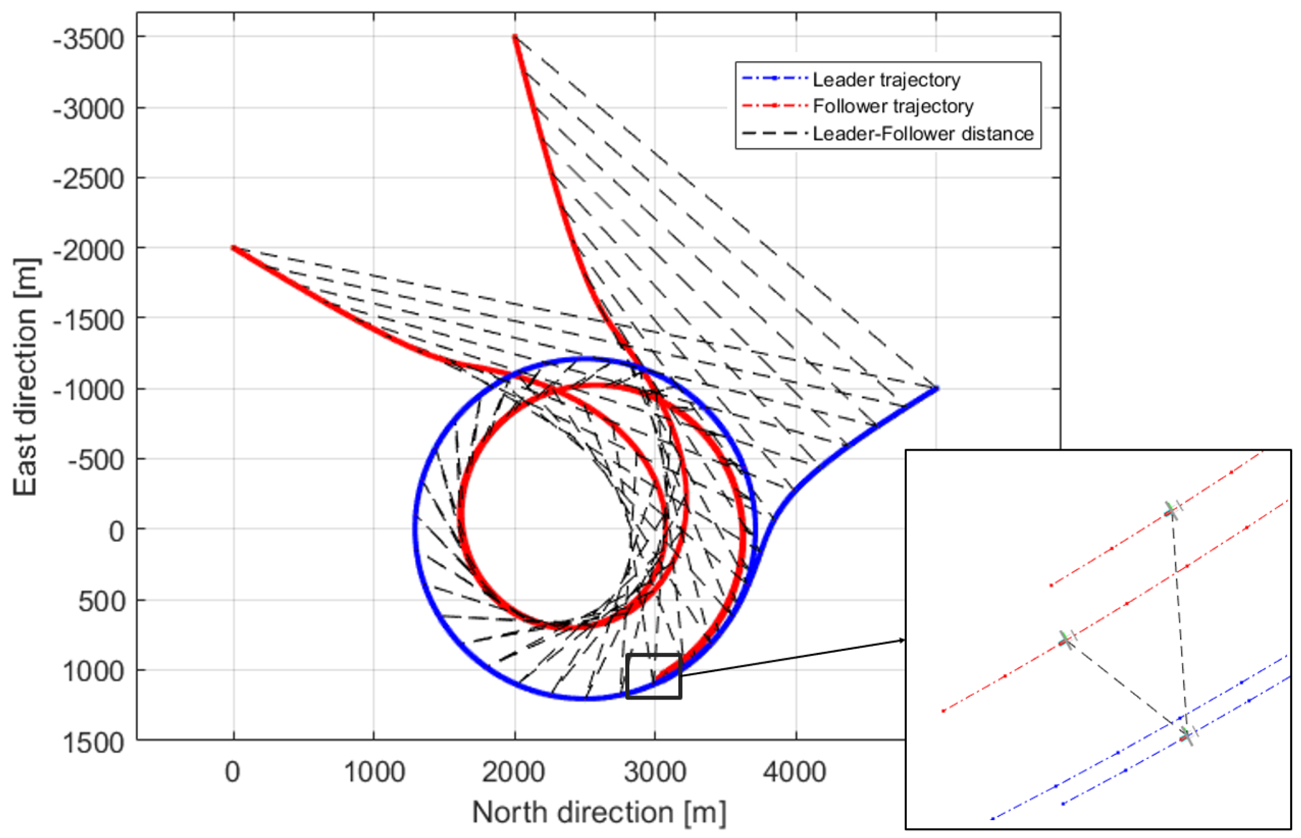
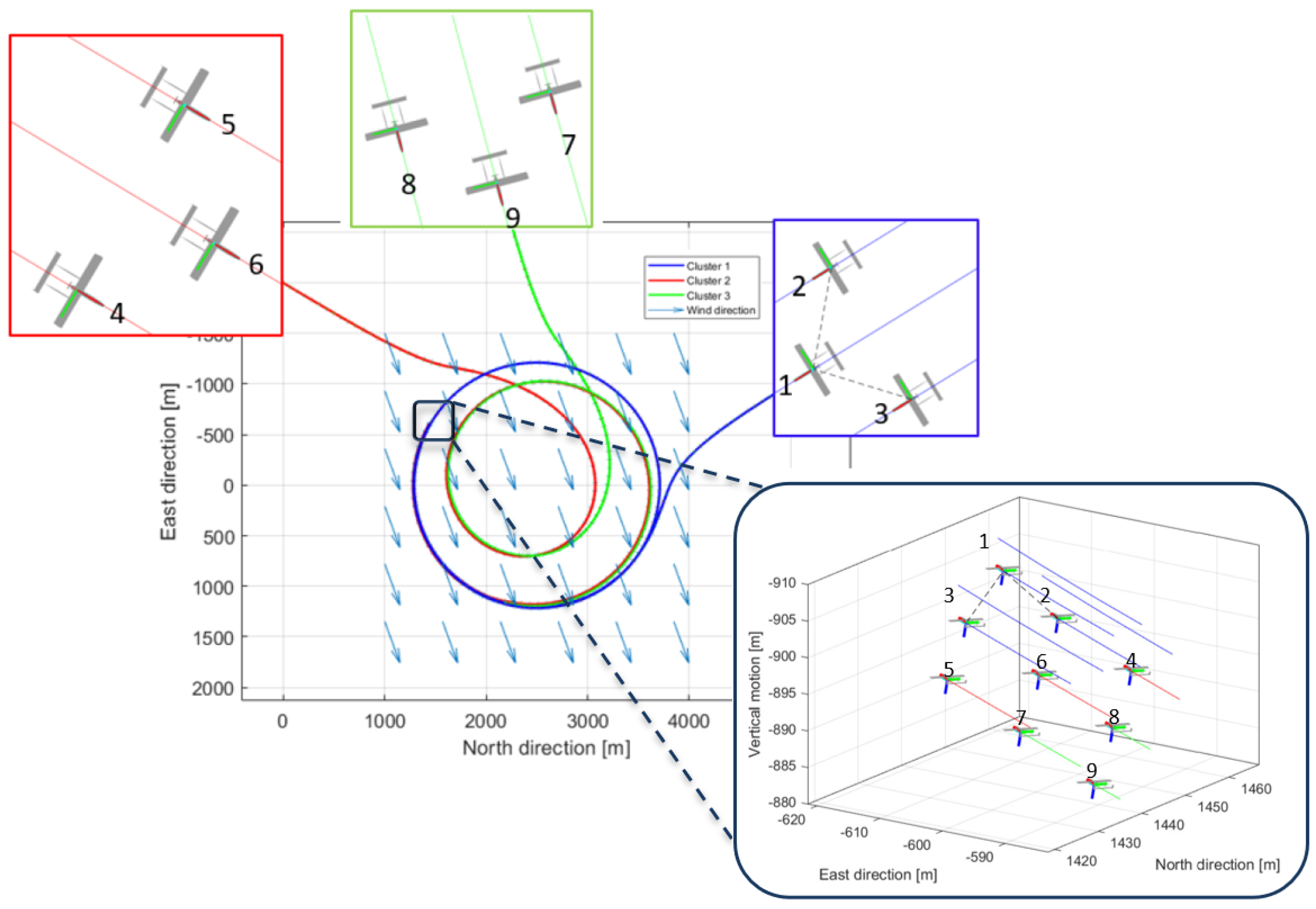
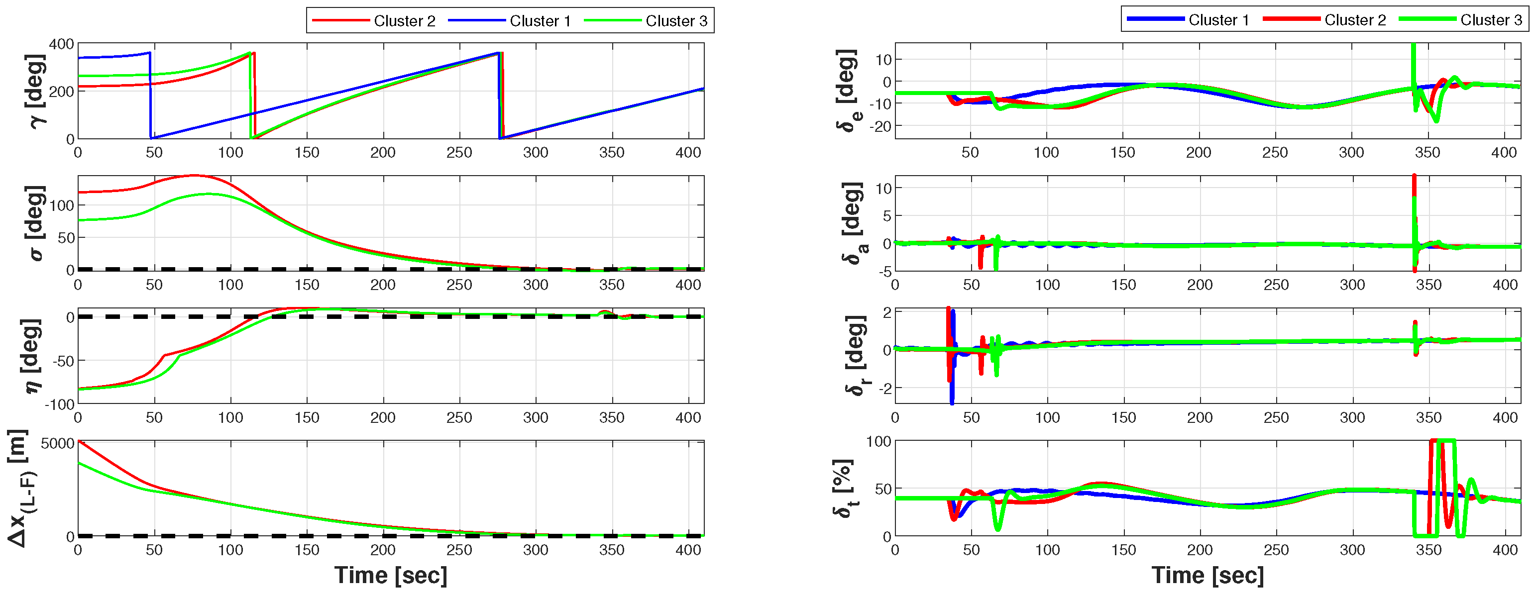
5.2. Rendezvous Testing

In this section, we describe how the proposed procedure for a formation rendezvous was tested. This marks the first introduction of a scenario involving multiple aircraft, whose trajectories were co-simulated within the SILCROAD environment. At this stage, they were non-cooperative entities. As shown in Figure 26, one aircraft was designated as the leader (in blue) and was placed on the assigned rendezvous orbit with a radius of $R=$ 1200 m and center coordinates at $\mathbf{c}=[2500,0]$ m. Two followers (in red) approached the orbit from different directions. As they neared the entry into the orbit, the rendezvous procedure was engaged, guiding the followers onto a tighter circular path until they completely achieved the phase shift of the leader. An event function was employed to halt the simulation once both followers were within 50 m of the leader.

The control authority over the rendezvous procedure is outlined in Figure 27. In the left plot, the resulting roll angles during the maneuver are compared to the commanded set points (dashed lines) for both followers. Contextually, the right plot illustrates the respective aileron control inputs for each follower. Initially, within the first 50 s time frame, the guidance system operated in the course-angle-tracking mode (vector field-based), rendering the roll angle completely independent of the set point. After crossing the proximity threshold for the distance from the target orbit, which was fixed in this case at $\widehat{d}=$ 250 m, the engagement of the roll angle control loop triggered an aileron impulse, initiating set point tracking.

The prescribed maneuvering procedure guaranteed the gradual approach of the followers to the leader, reducing the phase angle and stabilizing them on the target orbit once the appropriate positioning for formation assembly was attained, as shown in Figure 28.

A second test was conducted to assess the guidance system, with the addition of velocity control to reduce the convergence times (Equation (43)). The simulation result is shown in Figure 29, where it immediately becomes apparent that, under the same initial conditions, the matching point was significantly anticipated, as expected.

In this case, the graphs related to the resulting roll angles compared to the set point and their associated aileron inputs are shown in the top-left plot in Figure 30. Additionally, for this case, graphs related to velocity set point tracking and their respective throttle inputs are included (mid-left plot in Figure 30).

The control authority for roll angle tracking is perfectly comparable to the previous case. Concerning the velocity control modification, the guidance mode switch also affected the autothrottle, which set an impulse that reached saturation for a few seconds at the beginning of the set point tracking.

In conclusion, the set of parameters that collectively describe the followers’ leader-approaching maneuver is shown in the bottom plot in Figure 30.

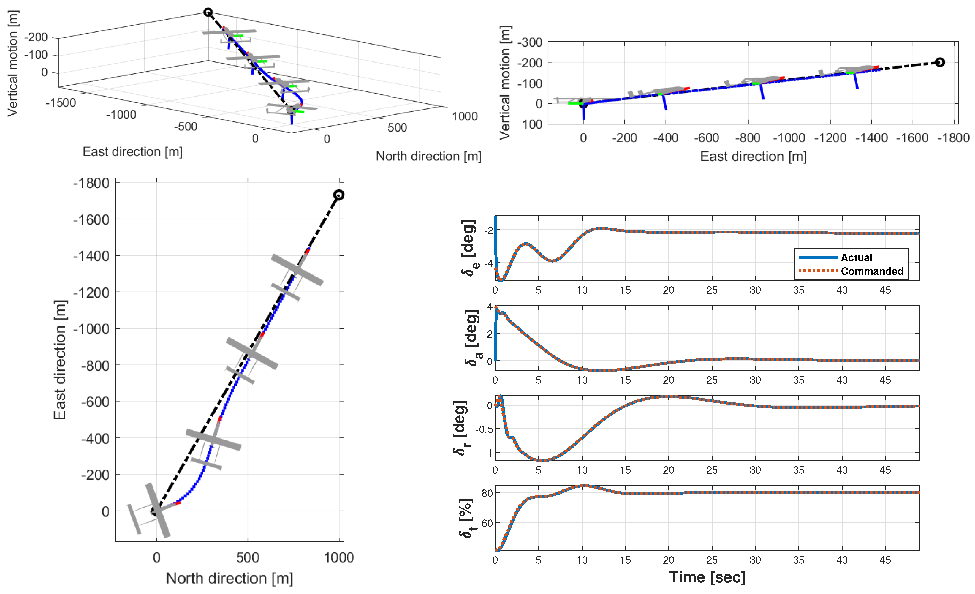
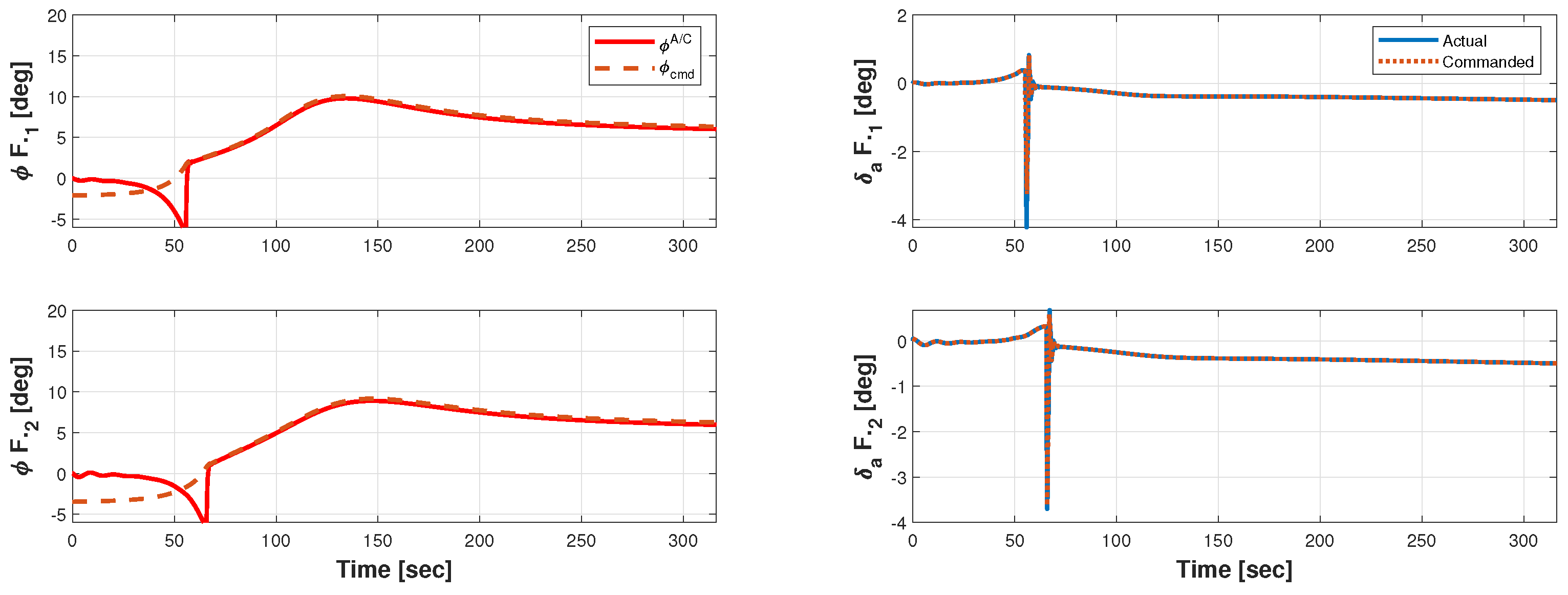
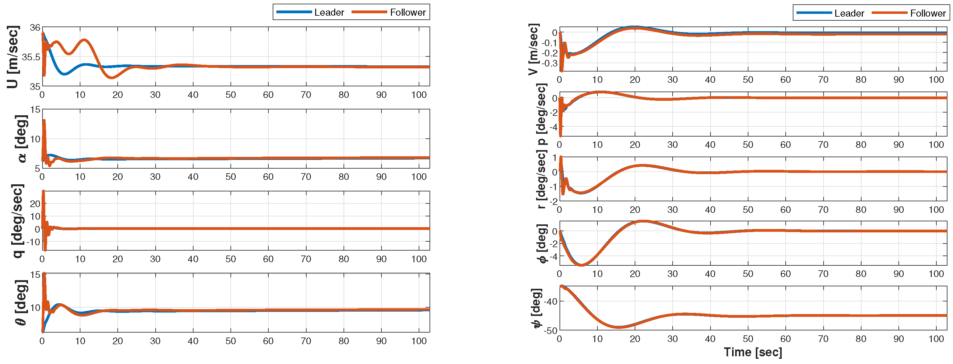
5.3. Formation Flight Testing Along a Rectilinear Leg

We then further increased the complexity of the simulation by introducing cooperative agents. As outlined in Section 3, the computation of dynamic parameters must account for wake interference, which, although modeled using the vortex lattice method (VLM), effectively captures the substantial alteration of the aerodynamic field experienced by trailing aircraft. This phenomenon not only impacts the selection of control parameters necessary for formation keeping, but it also justifies the relative positioning of the aircraft within the formation. Lookup tables for the aerodynamic delta-coefficients were generated through an analysis cycle using Tornado [43] software (release 136.7).

As shown in Figure 31, initially a symmetric wing geometry was defined, with the wing reference point (located at the mid-point of the leading edge) fixed at the coordinates $[7,0]$ m. This geometry represented the lifting surface of the trailing aircraft. An initial analysis was performed to determine the aerodynamic coefficients under isolated flight conditions, with the flight state set to a fixed angle of attack ($\alpha =$ 6 deg), a zero sideslip angle ($\beta =$ 0 deg), and an airspeed of 36.11 m/s, corresponding to near-optimal efficiency conditions.

Subsequently, an identical wing geometry was placed upstream of the first. The position of this leading wing was varied horizontally and vertically, generating a matrix of values: rows represented the lateral separation between the two wings, $(\Delta y)$, while columns represented the vertical separation, $(\Delta z)$. The stream-wise distance $(\Delta x)$ was initially kept constant.

The software provided aerodynamic coefficients for each lifting surface separately. The effect of wake interaction was quantified by subtracting the coefficients of the isolated trailing wing from those of the trailing wing in the tandem configuration. Figure 31 introduces an insight into the outcome, illustrating the variations in the aerodynamic coefficients for the trailing wing (for brevity, only $\Delta C_L$ and $\Delta C_D$ are reported) across a range of lateral and vertical separations spanning from −20 m to 20 m. The stream-wise direction distance was set to 7 m.

The regions where peaks in the lift coefficient ($\Delta C_L$) and valleys in the drag coefficient ($\Delta C_D$) were observed corresponded to the optimal conditions (sweet spot) mentioned earlier. This region was found when the two lifting surfaces had no vertical stagger and a lateral separation of just over 5 m (approximately 5.15 m), which corresponded to the length of a wingspan. Assuming the lateral separation as the distance measured between the wing reference points, the sweet spot for the trailing aircraft corresponded to having its wingtip aligned with the wingtip of the leading aircraft in a stream-wise direction.

Two-Aircraft Formation: Single-Leg Trajectory Path. A preliminary testing phase was conducted considering two aircraft, assigning a single straight-and-climbing flight path to the leader, while the follower was instructed to maintain a 6 m distance from the leader along all three reference axes, starting from a non-zero positional error. In addition, an initial misalignment of 10 deg from the desired course was imposed to test the formation control system’s capability to counteract a sudden change in the climb path and lateral course deviation. The trajectories are shown in Figure 32.

Looking at the right plot, the follower responded to the initial disturbance in a more abrupt manner, aiming to quickly catch up not only with the target position but also with the leader’s attitude. However, none of the four control commands reached saturation, thereby ensuring a wide maneuvering margin for the follower aircraft. It is noteworthy that while the elevator, rudder, and throttle tended to converge to the leader’s values after the realignment maneuver, the aileron retained a residual value different from zero. This was expected, since the aileron compensates for the rolling moment induced by the wake interference.

The overall assessment of the formation performance could be carried out by evaluating the three characteristic errors, reported in Figure 33, targeted by the formation control system in cruise mode (${\mathit{e}}_{\mathit{P}\mathbf{1}},{\mathit{e}}_{\mathit{P}\mathbf{2}}$, and ${\mathit{e}}_{\mathit{P}\mathbf{3}}$).

The formation control system demonstrated satisfactory performance, reducing both the vertical and longitudinal position errors to zero in physically acceptable time windows. The persistent lateral error ${\mathit{e}}_{\mathit{P}\mathbf{2}}$ can be attributed to the equilibrium condition established by the aircraft to compensate for the wake-induced rolling moment. All positional errors converged to a constant value within a tolerance band of ±2 m.

From Figure 34, which depicts the time evolution of the states of the leader and follower, it is evident how the follower effectively adapted to the new flight condition imposed by the leading unit, generating an almost identical response for both longitudinal and lateral–directional dynamics.

Three-Aircraft Formation: Triangular Pattern. In this scenario, the formation was tested on a triangular circuit with 60 deg angles at the vertices. The aim was to assess the stability of the formation at the turning points and observe how the formation was recovered once the leader had realigned with the next leg. The trajectories and control time histories are reported in Figure 35.

Overall, the control system ensured satisfactory formation recovery, with the followers reaching and maintaining their assigned target positions beyond the turning points (see Figure 36). The turn rate required for heading changes created some challenges in maintaining the geometry of the formation. In particular, the left follower (on the outer edge of the turn) struggled to maintain the correct lateral position, while the right follower (on the inner edge of the turn) made a substantial effort to maintain the correct longitudinal position, as observed in the corresponding time history of the throttle.

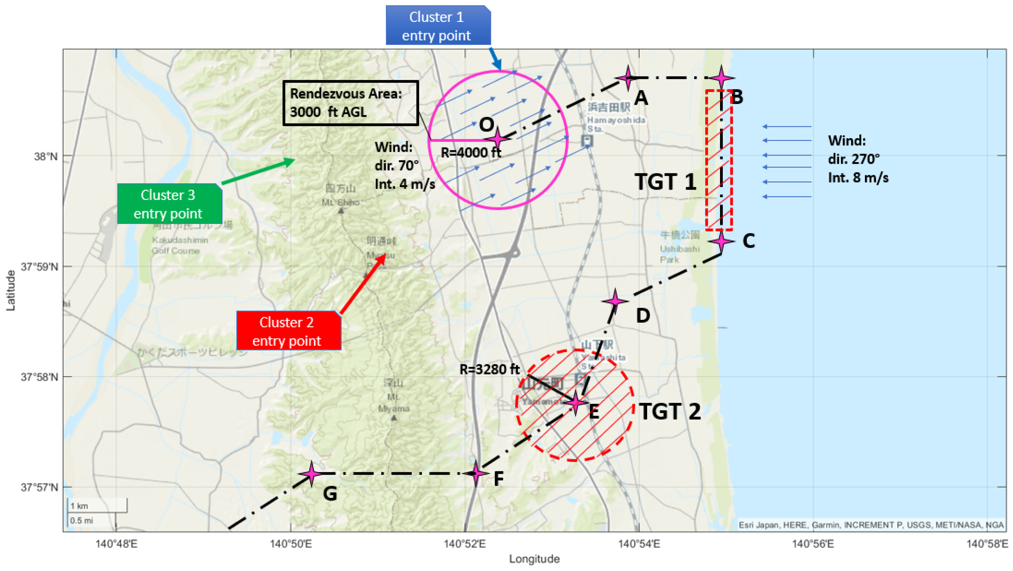
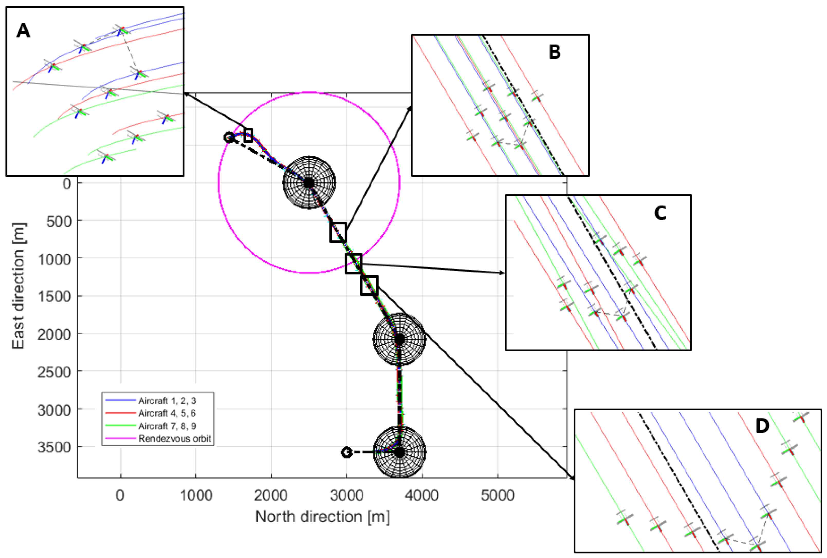
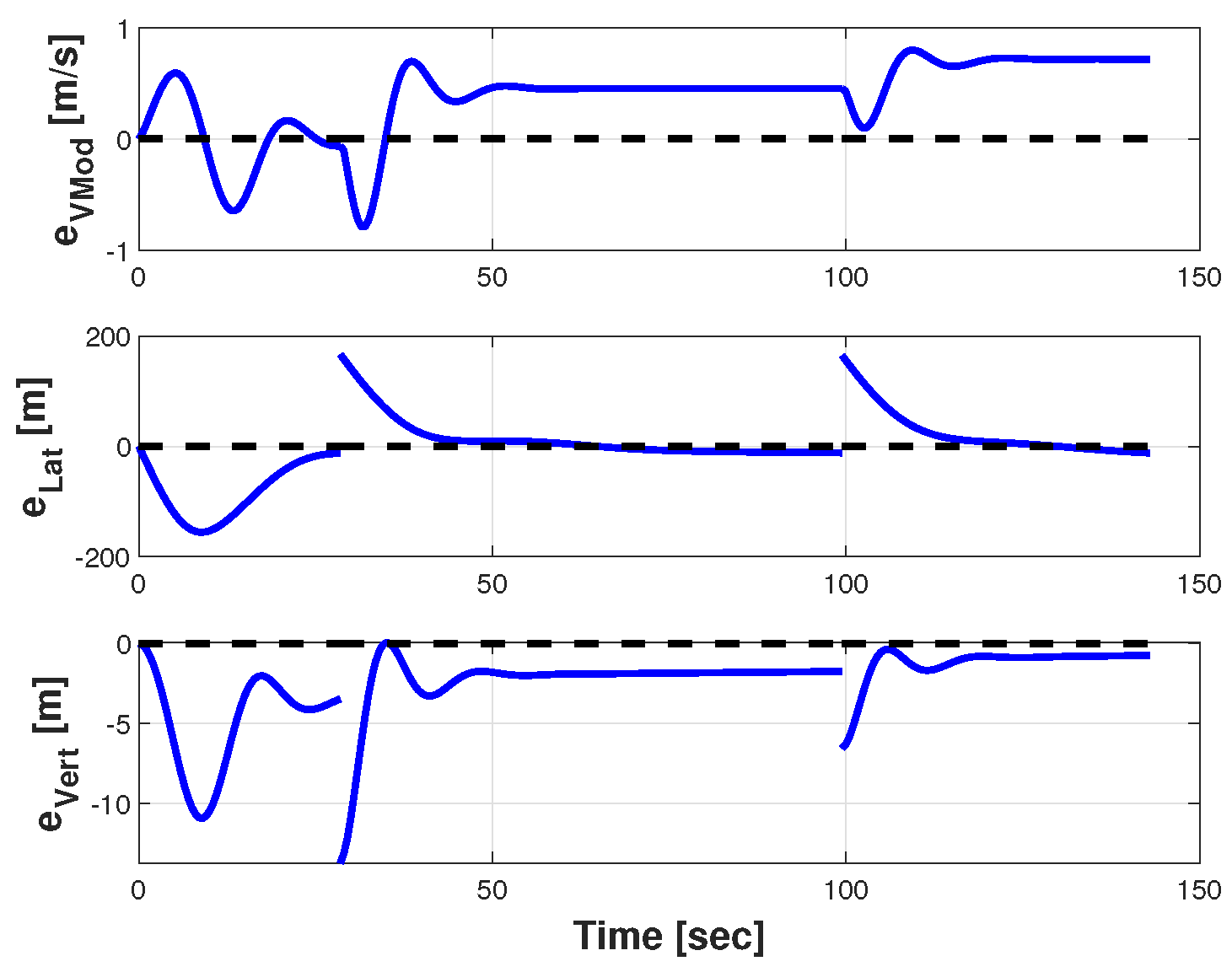
5.4. Realistic Mission Simulation

Following the formulation and validation of control laws for guidance and formation maintenance in specific test scenarios, it became feasible to design a complex mission scenario that demonstrated the full spectrum of capabilities offered by the simulation tool under consideration. This section comprehensively explores the utilization of fixed-wing UAV swarms dropped into the 2011 Fukushima disaster context. We delve into the design, planning, and execution of a simulated mission in the Fukushima region, emphasizing the adaptable and collaborative nature of UAV swarms to address the evolving needs of disaster response.

The mission was carried out using nine aircraft organized into three clusters. The mission objective was to fly over a stretch of coastline damaged by the tsunami and loiter around the small town of Yamamoto, acquiring photographic material needed by ground units to coordinate rescue efforts. A detailed mission schedule is provided in

Table 1. Mission schedule.

Rendezvous
Orbit center	Orbit radius	Altitude	Velocity	Additional notes
38°01′ N, 140°53′ E	1200 m	900 m	120 km/h	Wind: ${\psi }_w=135$ deg, int. 4 m/s
Waypoint navigation
Leg	Length	$\Delta h$	Velocity	Additional notes
O-A, $\psi =60$ deg	2400 m	$-200$ m	130 km/h	Formation geom. switch—V.
A-B, $\psi =90$ deg	1500 m	$-100$ m	130 km/h	-
B-C, $\psi =180$ deg	3100 m	$-100$ m	130 km/h	Wind: ${\psi }_w=270$, int. 8 m/s
C-D, $\psi =240$ deg	2000 m	$+100$ m	130 km/h	Formation geom. switch—D.
D-E, $\psi =200$ deg	2000 m	$+0$ m	130 km/h	-
Loiter
Orbit center	Orbit radius	Altitude	Velocity	Additional notes
37°57′ N, 140°53′ E	1000 m	400 m	120 km/h	-
Waypoint navigation
Leg	Length	$\Delta h$	Velocity	Additional notes
E-F, $\psi =240$ deg	2000 m	$+200$ m	130 km/h	Formation geom. switch—V.
F-G, $\psi =270$ deg	2600 m	$+200$ m	130 km/h	-

, while the main navigation information is reported in Figure 37. In the preliminary phase, one unit was designated as the leader for each cluster, responsible for guiding the three-aircraft formation to the rendezvous area and overseeing the formation-rejoining process. The rendezvous area was situated near the coast. Cluster 1 was scheduled to depart from Yamagata Airport, located to the northwest of the target area. Cluster 2’s departure was planned from Fukushima Airport, positioned to the south of the designated zone. Meanwhile, the third cluster was already airborne, heading from the west towards the rendezvous point. The target area was situated between a mountain range with medium–low orography (summit point at 690 m) and the coastline, necessitating some precautions. To reach the rendezvous point, it was necessary to fly over the mountain range with a safety margin of at least 200 m above the summit. The rendezvous was, therefore, conducted at an altitude of 900 m above ground level (3000 ft). Additionally, due to the topographical layout, the area was prone to moderate-intensity winds, both near the area with greater terrain relief and along the coastal stretch.

Among various potential solutions, two formation geometries were selected for this mission type. The first was a V-shaped formation for navigation phases, while the second was a diamond-shaped formation for target overflights. The interchangeability between these two geometries could be controlled based on either time or the inertial coordinates. Once the formation geometries were defined, a choice needed to be made. Either each follower would be linked to a unique leading unit, or the positions would be linked in a chain so that each aircraft was the direct follower for the preceding unit. The first solution was pursued primarily because this approach provided rigidity to the formation (in the second case, any positioning errors of more advanced followers would propagate throughout the swarm).

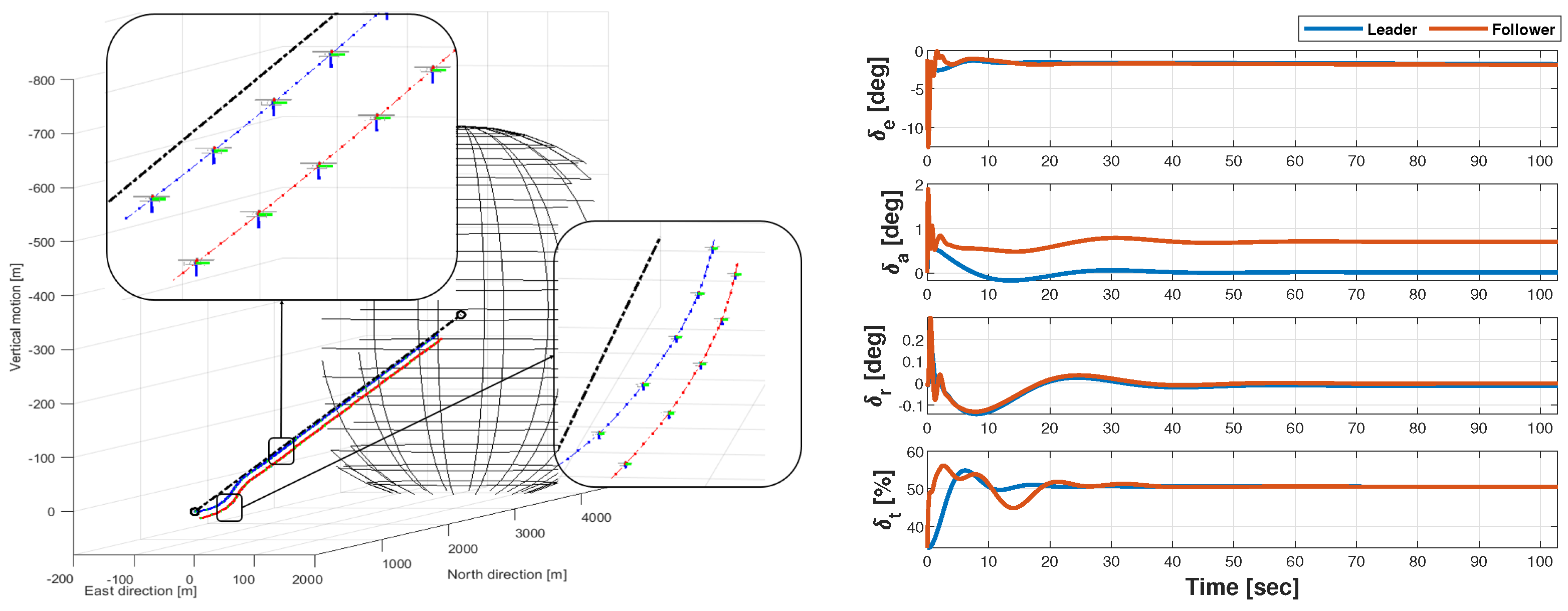
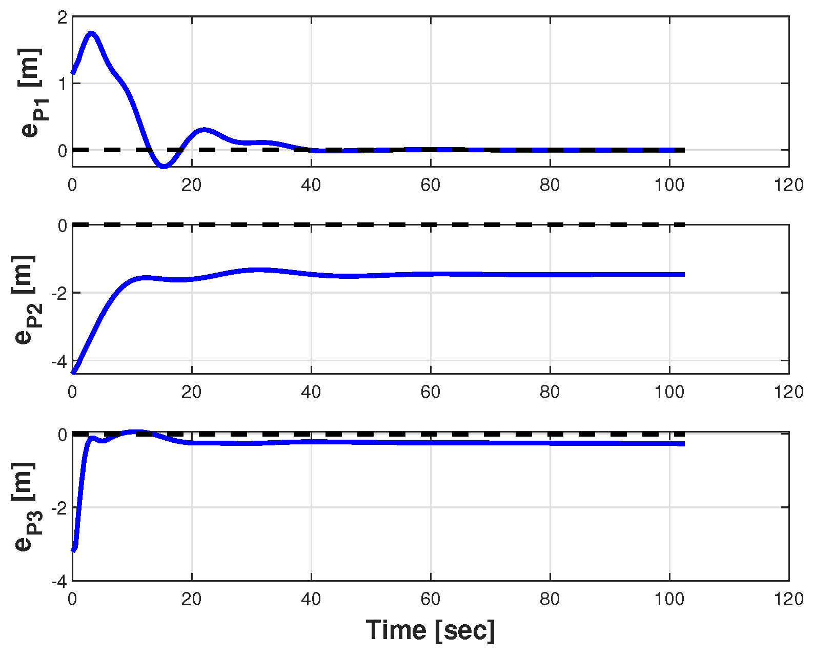
5.4.1. Phase 1: Rendezvous

The rendezvous procedure followed the control logic discussed in Section 4.1.4, placing Aircraft 1, the designated swarm leader and leading unit of Cluster 1, on a circular orbit with a radius of $R=$ 1200 m at an altitude of 900 m (Figure 38). Aircraft 6 and 9, the leaders of Clusters 2 and 3, respectively, gradually integrated into the approach trajectory, chasing Aircraft 1. The three clusters flew with a vertical separation of 30 ms to prevent mid-air collisions during formation rejoining. When they were within 40 m of relative distance from the formation leader, the Flight Control Mode (FCM) was engaged for all followers, causing them to acquire their target positions relative to Aircraft 1.

The relative distance between the leader and followers 1 and 2 is marked with a black dashed line to visualize the vertex of the formation once reassembled without cluttering the plot.

The procedure was executed without speed control, so in general, the approach of the clusters occurred rather gradually. This was performed to ensure that the phase difference to Cluster 1 was not eliminated too quickly. In such a case, the followers would be at the same phase angle as the leader but at a relatively large distance to engage the FCM without the need for abrupt repositioning maneuvers.

As shown in the left plot in Figure 39, displaying the control parameters for the rendezvous procedure, the approach proceeded appropriately despite the presence of the crosswind. Phase shift recovery was achieved within 270 s of entering the rendezvous area. In the subsequent time window, the clusters gradually reduced their relative distances until they achieved complete formation rejoining in a diamond shape.

A quick glance at the right plot in Figure 39 reveals how the rendezvous phase was managed in terms of control. The rapid control oscillations between 50 and 70 seconds represent the intervention of the guidance and stabilization systems upon entering the wind-disturbed area. Importantly, this disturbance did not significantly impact the execution of the procedure, as indicated by the relatively smooth control inputs until FCM engagement for Clusters 2 and 3 at around 340 s. It is evident that the FCM switching on at this point resulted in a sharp throttle response to adapt the followers to the leader’s longitudinal position and velocity. Nevertheless, the repositioning was completed without significant issues. One potential amelioration could involve managing the final phase of the approach by imposing a velocity correction on the leader as well, in order to accommodate formation repositioning.

5.4.2. Phase 2: Waypoint Navigation

The navigation phase involved the swarm departing from the rendezvous orbit to head towards the first waypoint at the orbit center. While traveling along the second leg, a reconfiguration of the formation into a V-shape was commanded, as depicted in Figure 40.

The formation remained compact behind the leader even during more pronounced maneuvers, such as the turn towards the first waypoint.

The beam-tracking errors targeted by the leader are shown in Figure 41, but what was more interesting to test was the ability of the formation to reconfigure itself. Figure 42 displays the position errors and the corresponding command time histories for Aircraft 6, 7, 8, and 9, which underwent a positional change. In particular, Aircraft 6, positioned centrally in the diamond-shaped formation, assumed the role of the third-right follower in the V-shaped configuration. Aircraft 7, 8, and 9, representing the rear vertices of the diamond-shaped formation, respectively took positions as the third-left follower, fourth-right follower, and fourth-left follower at the edges of the V.

Despite the initial struggle to maintain their position due to the abrupt course realignment maneuver, the positioning errors were effectively reduced following the reconfiguration request.

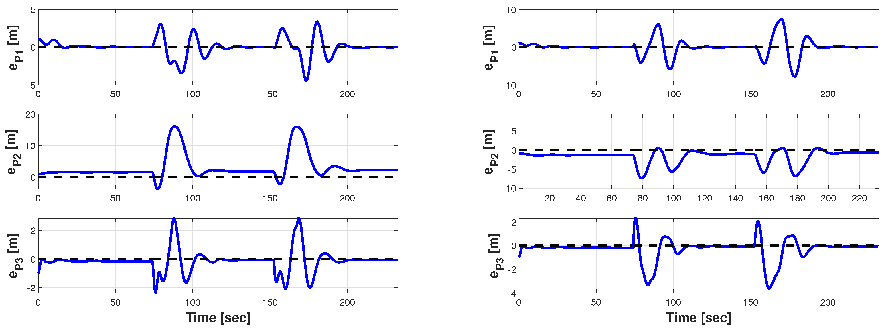
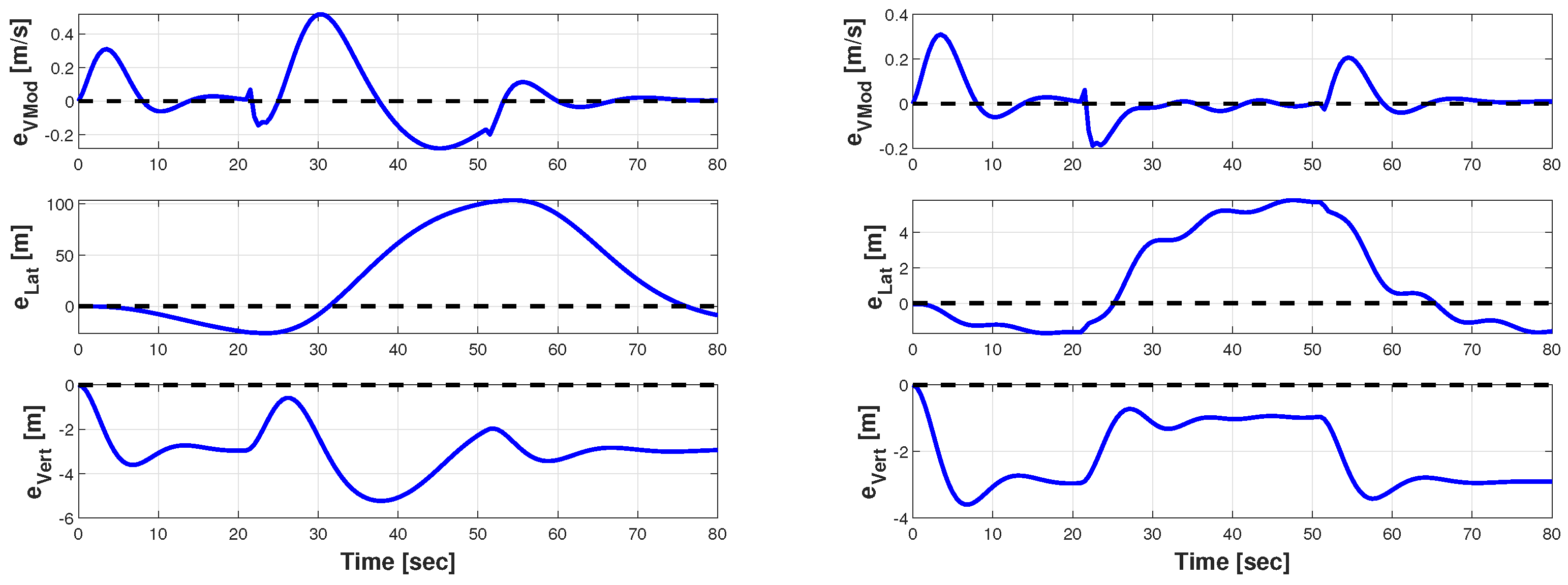
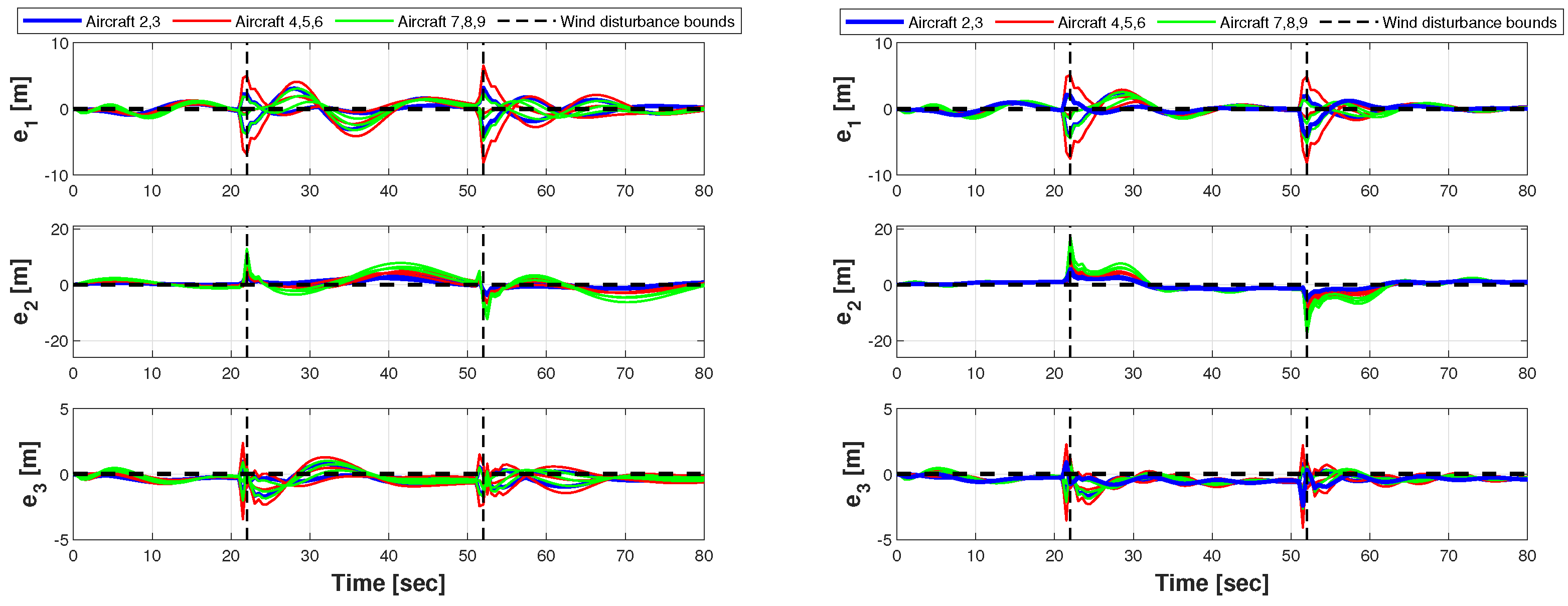
5.4.3. Phase 3.a: Target 1 Overflight with Crosswind

During the target overflight, the formation, which had been spread out to provide wider ground coverage, was subjected to a medium- to high-intensity crosswind.

In Figure 43, a comparison between the trajectories obtained without any compensation and with the crabbing maneuver performed by the leader is shown, along with time histories of control highlighting the crabbing maneuver coordination.

In this approach, when the leader entered the wind stream, it went into a skidding trim with a coordinated rudder input (based on lateral beam-tracking indicators) and an aileron counter-command (crabbing maneuver), effectively reducing the cross-track error (Figure 44, right).

The followers, controlled solely via the FCM, then tracked the leader’s velocity vector. This resulted in more efficient ground coverage with a significantly lower average cross-track error compared to the scenario without the leader’s correction (Figure 44, left).

In both cases, the formation remained relatively compact, with the position errors effectively reduced to zero, despite visible perturbations during the entry into and exit from the disturbance zone (Figure 45).

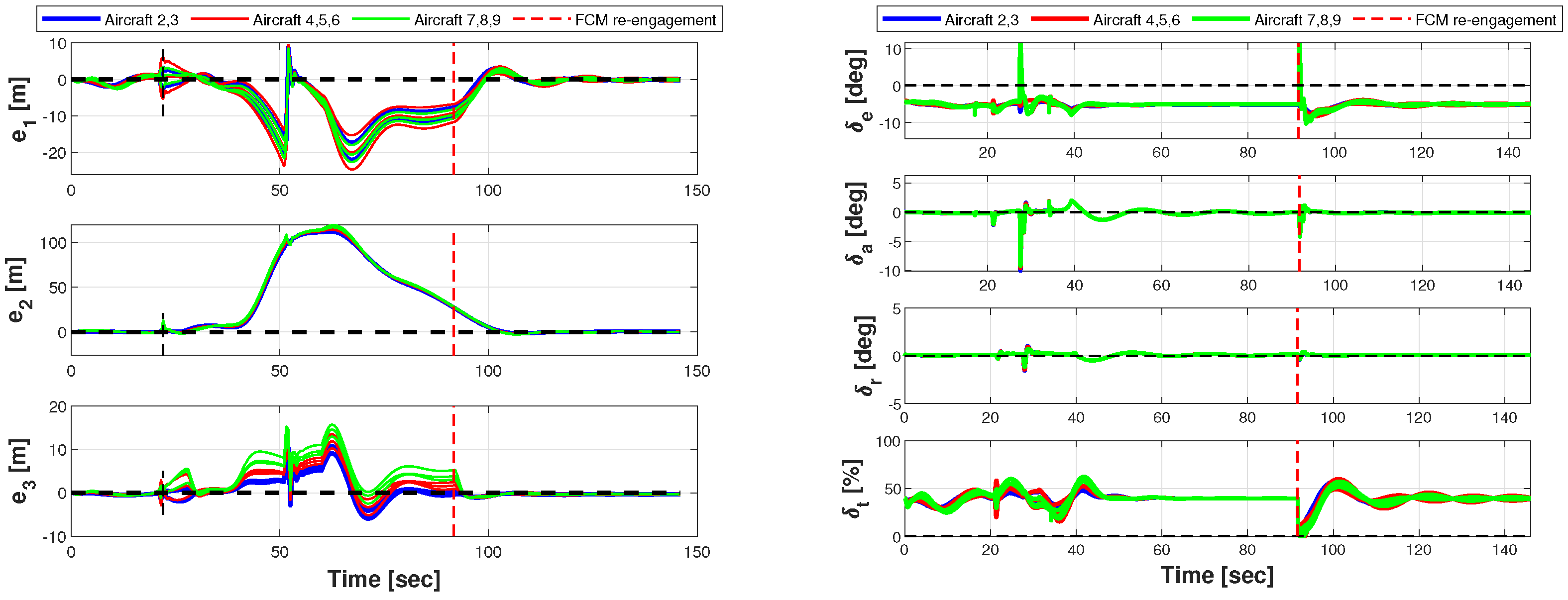
5.4.4. Phase 3.b: Target 1 Overflight with Leader’s Guidance Mode (GM) Failure

A parallel scenario was envisaged with respect to Phase 3.a. In this case, a failure in the leader’s guidance system was simulated, such that the aileron and rudder commands did not intervene to compensate for the increase in the cross-track error induced by the wind. The failure was extended for 25 s (from $t=$ 35 s to $t=$ 60 s), after which the guidance system regained authority, bringing the leader back onto the beam (Figure 46).

The follower’s autopilot managed the wind-induced disturbance by switching between the formation control (FCM) and guidance modes (GM). When the leader experienced a cross-track error over a predefined threshold, upon entering a wind stream, the GM took over to maintain the intended flight path for the formation. Once the disturbance subsided, the FCM was re-engaged to restore the original formation.

The transition between these modes was governed by a supervisory control which employed linear gain transition logic based on cross-track error thresholds and adjustable parameters (on the same basis as the trajectory blending vs. beam-tracking transition logic, shown in Figure 19). A higher transition rate proved advantageous only during the initial switch (from the FCM to the GM), as it engaged a control law tuned with lower gains. Conversely, a reduced transition rate was essential for the reverse switch to prevent abrupt position corrections that may have induced instability.

Beyond the 20 m threshold for the cross-track error, the supervisory control system detached the rest of the formation from the leader and returned its elements to their designated route.

Upon the leader’s repositioning, the supervisory system instructed the followers to reacquire their respective positions within the formation.

The set of position errors and their respective control histories for all the followers are depicted in Figure 47. This distinctly shows the phase of formation detachment and the re-engagement of the FCM, occurring at $t=$ 91 s.

A significant challenge may arise when the leader deviates by several meters, causing followers to struggle with longitudinal position recovery. This is due to the leader slowing down under a disturbance while followers maintain their ground speed. Upon the re-engagement of the FCM, abrupt throttle adjustments can result in oscillations and prolonged recovery times. A potential solution involves assigning the leader’s airspeed-hold loop control branch with two set points for both the position and velocity, derived from the longitudinal position error ${\mathit{e}}_{\mathit{P}\mathbf{1}}$ and velocity error ${\mathit{e}}_{\mathit{P}\mathbf{1}}^{\mathit{Vel}}$. This approach mirrors the autothrottle logic of the FCM, but with inverted gain signs. When ${\mathit{e}}_{\mathit{P}\mathbf{1}}>0$ or ${\mathit{e}}_{\mathit{P}\mathbf{1}}^{\mathit{Vel}}>0$ (followers lagging behind the target position), the followers accelerate while the leader decelerates. Conversely, for ${\mathit{e}}_{\mathit{P}\mathbf{1}}<0$ or ${\mathit{e}}_{\mathit{P}\mathbf{1}}^{\mathit{Vel}}<0$ (followers ahead of or converging toward the target), the leader accelerates while the followers decelerate. This strategy ensures the rapid and smooth correction of longitudinal positions across the formation, avoiding command saturation.

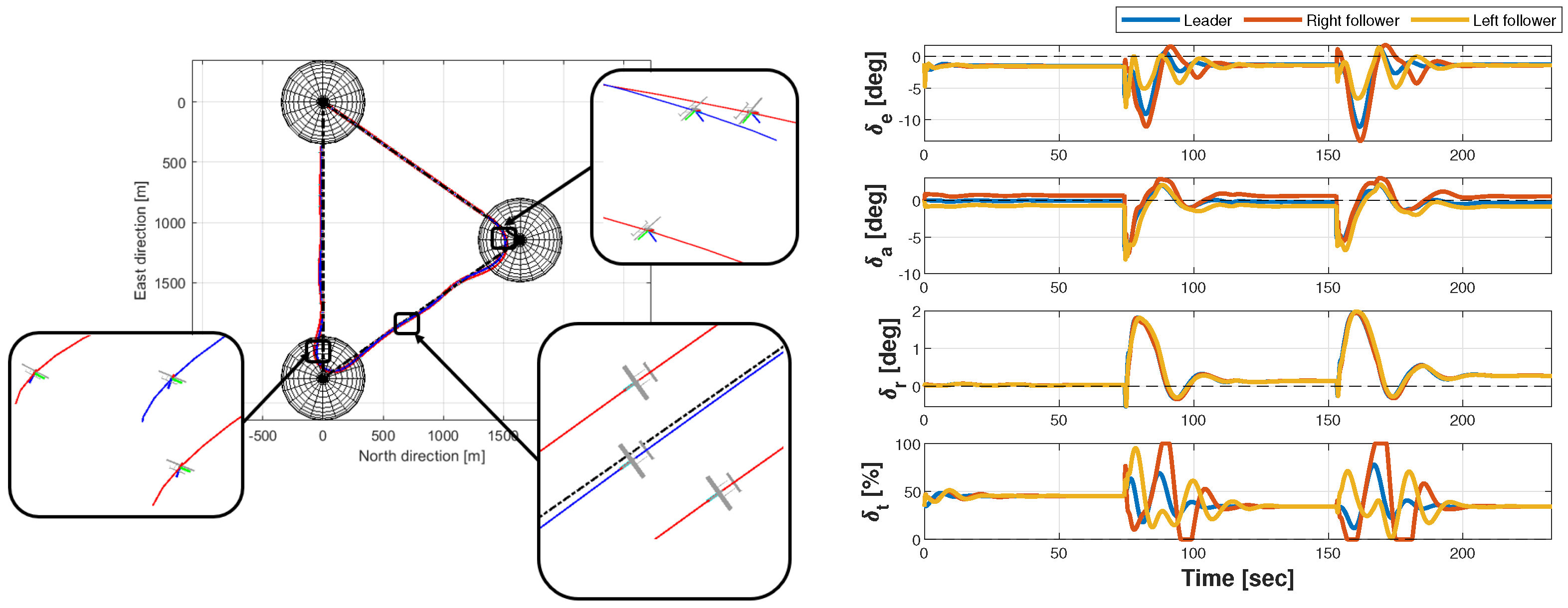
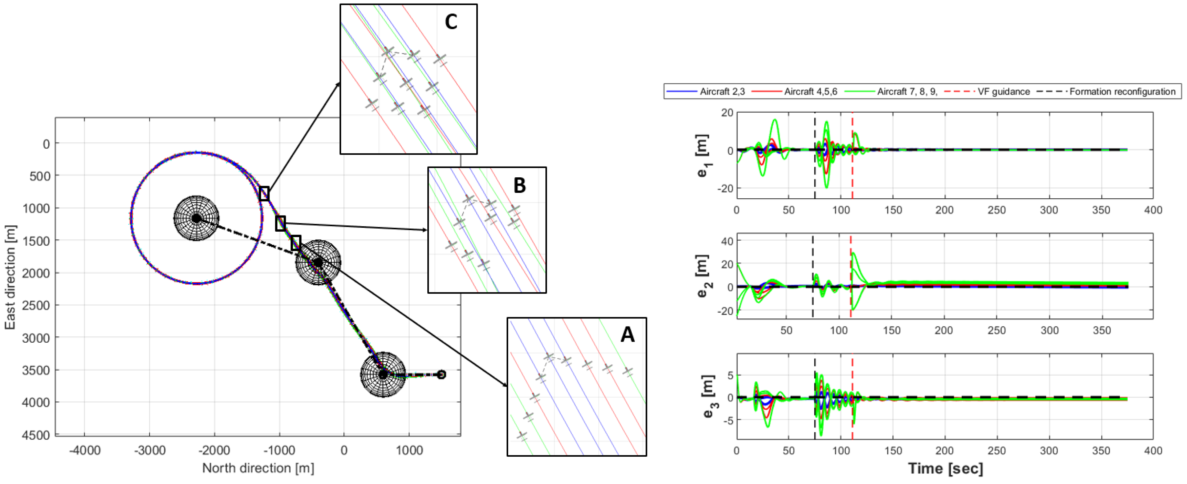
5.4.5. Phase 4: Target 2 Overflight

The formation, after completing the overflight of the first target in the V configuration, reverted to the navigation route to reach the second target. At the end of the second leg of the path, the guidance system initiated the tracking of the vector field of the course angles to enter the orbit with a rather relaxed transition rate. Before entering it, a new configuration change was commanded, from a V to a diamond shape (Figure 48).

No significant issues were observed for the guidance system tracking performance.

A minor issue affecting the rest of the formation emerged during the transition to the vector field-based guidance mode. If the aircraft were not well aligned with the direction of the vector field at the moment of transition, the guidance system generated a strong response to align the leader with the commanded route. This led to a series of oscillations in the position tracking of the followers, which could be particularly challenging for the rearmost aircraft experiencing wider oscillations (right plot in Figure 48). Despite this, the geometry reconfiguration of the formation was successfully achieved, and the position error of the followers stabilized near zero for the remainder of the target overflight.

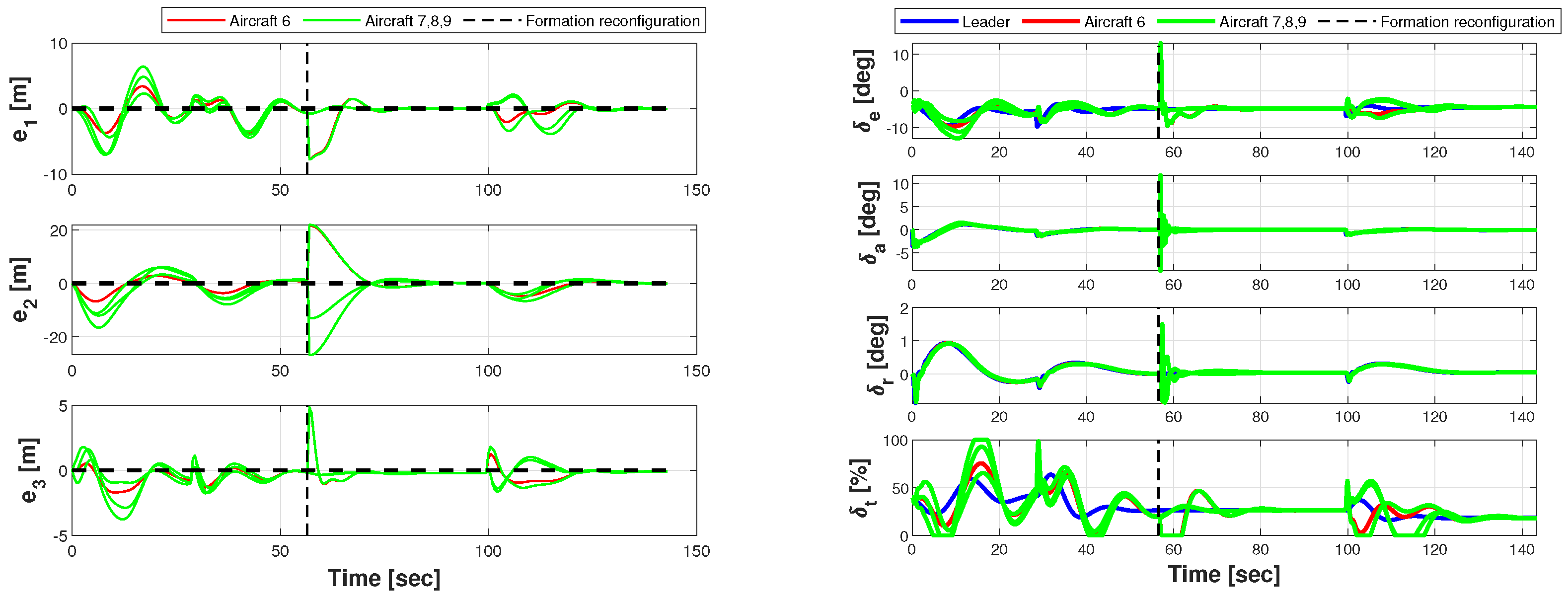
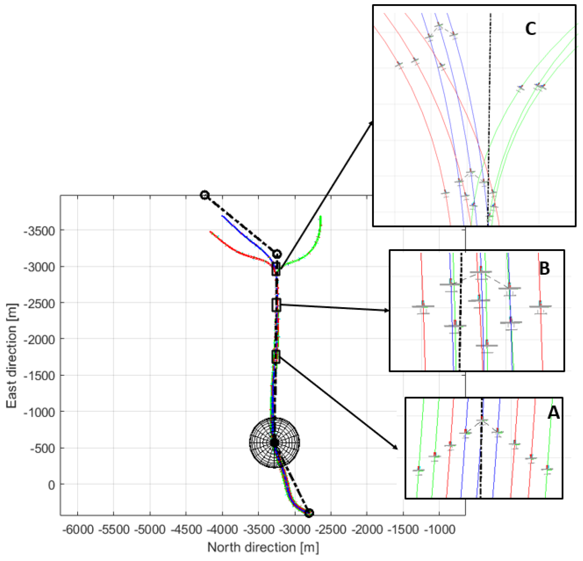
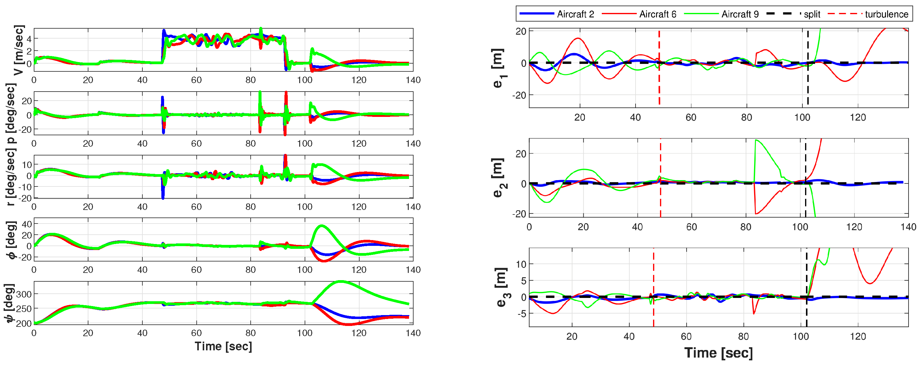
5.4.6. Phase 5: Disengagement and Formation Splitting

The final phase of the mission involved the disengagement of the formation from the operational area. The formation was directed onto an exit trajectory that included traversing a turbulent zone along the path of the second leg (Figure 49). Within the simulation, turbulence was modeled using a random signal with specified lower and upper bounds. In this instance, the deterministic wind component was fixed at 4 m/s, with turbulence occurring within ±1 m/s.

The effect of turbulence is clearly visible in Figure 50, where the lateral–directional states for Aircraft 2, 6, and 9 are shown as examples, representing the behavior of the entire formation.

Despite this, the formation retained compactness without the development of dangerous instabilities. The only issue also present in this case was that the outermost members of the formation struggled to maintain the correct longitudinal position (see the right plot in Figure 50) during sharp turns (first maneuver when exiting the circular orbit).

Shortly before splitting, the formation reconfigured into a diamond shape, bringing the aircraft belonging to the same cluster closer together. Afterwards, Aircraft 9 and 6 were designated as the leaders of their respective clusters, while the others acquired their target positions relative to their cluster leader. The separation occurred smoothly.

6. Conclusions

Various aspects of formation flight have been investigated within this work. The intent was not to replace the existing documentation on the control and coordination of a multi-unit fixed-wing UAV system, but rather to propose a viable alternative for the more in-depth modeling of the problem from the perspective of flight dynamics, rather than pure control architecture. Dynamic modeling in a fully nonlinear environment has allowed for the highlighting of specific aspects of the problem at hand, such as the stability of individual aircraft subjected to state disturbances, the challenges of interfacing with nonideal actuation systems subjected to bandwidth limitations and signal saturation, the effects induced by aerodynamic interaction, and the criticality of maneuvering at angles of attack close to stall while avoiding exceeding the constraints on the minimum sustaining airspeed, as well as managing a limited available engine power, resulting in a constrained flight envelope.

The problem of stabilization was addressed by employing a Stability Augmentation System (SAS), designed following a model-based approach and tuned according to an LQR (Linear Quadratic Regulator) procedure. This approach resulted in satisfactory three-axis stabilization, ensuring the required flying qualities for the specific aircraft class and leaving sufficient bandwidth for the higher layers of the controller responsible for guidance.

A guidance system was studied to ensure the capability of the swarm to follow a path with multiple checkpoints in 3D space, adjusting the aircraft’s heading and altitude to accommodate realistic navigation requirements. The chosen control logic and tuning ensured adequate guidance system performance, tested on several polygonal patterns, where the cross-track error was effectively reduced to zero for each leg. Additionally, the system was able to avoid trajectory overshoots thanks to the blending technique employed.

The vector field-based guidance procedure provides an effective solution for executing loiter maneuvers and facilitating formation regrouping within confined spaces. In this regard, its integration with a specific rendezvous guidance protocol based on followers re-phasing, by means of a lateral acceleration set point, expedites the formation rejoining times and mitigates the issue of a limited available speed range, which is crucial for linear rendezvous execution.

For formation coordination, a control architecture based on the leader–follower hierarchy was employed. A decentralized control approach was adopted, where each aircraft (follower) is assigned a target position to chase, relative to the preceding aircraft (leader). This is achieved by comparing the position, attitude, and trajectory information exchanged between the two involved formation agents. This communication mode ensures a limited amount of exchanged data, thereby reducing the computational complexity and required communication bandwidth and consequently ensuring swarm scalability. The outcome of the performed testing demonstrated effective and promising formation coordination. The follower aircraft were able to maintain a stable (within proper tolerances) and aligned position relative to the leader aircraft, responding appropriately to variations in the leader’s position and trajectory. Additional tests were performed to assess the formation behavior in the presence of a constant wind disturbance, ensuring a tight formation through relative position tracking within the swarm, or triggering formation reconfiguration, with followers flying along a designated route when properly switching their autopilot mode.

A realistic scenario was envisaged in order to test the synthesized controllers dropped into an operational context typical of a ground reconnaissance mission.

The objective was to test the feasibility and reliability of a swarm with a scaled number of units and complexity, placed within a realistic operational context. The ensemble of control algorithms proved capable of conducting all the distinct phases of the mission without significant issues. The required variations in the altitude and speed conditions did not pose problems for the stabilization system, enabling individual aircraft to operate even in the presence of induced disturbances. The guidance procedures facilitated the seamless execution of different mission phases, while the formation control system demonstrated its suitability for coordinating the formation, adapting effectively to substantial trajectory changes made by the leader and responding to formation reconfiguration requests.

In summary, this investigation has provided a thorough and realistic exploration of each operational phase within an unmanned multi-element formation flight mission. This underscores the sophistication of our analytical tool, offering the capacity to conduct comprehensive assessments of missions of this nature with a high degree of fidelity and realism.

Future Perspectives

There are several perspectives for the further development of this work currently under consideration:

• Firstly, the possibility of significantly increasing the number of aircraft units within the swarm while establishing a proper hierarchy to ensure stability and robustness.
• Secondly, an analysis of potential swarm reconfiguration strategies in case of signal loss. For future research, an exploration of coordination logic based on local distance measurements using lasers, as opposed to relying solely on GPS data, could be pursued. This approach not only mitigates the risk of signal interception but also holds promise for enhanced operational security in military contexts.
• The potential implementation of additional control techniques for collision avoidance, both among swarm units and with environmental obstacles, as well as guidance strategies aiming at the mitigation of risk and discomfort induced by the overflight of unmanned machines and by noise, respectively, could represent a significant contribution to this research domain. These techniques and strategies aim to refine automation and enhance the system reliability in increasingly complex scenarios.
• Lastly, the optimal tuning of the control systems could be pursued to enhance their performance across a wide range of deployment scenarios. This could involve conducting extensive simulations to identify the optimal control settings and refine the control algorithms with the aim of maximizing the effectiveness, efficiency, and adaptability of the control systems in different mission scenarios.

References

1. Liu, Z.; Wang, X.; Shen, L.; Zhao, S.; Cong, Y.; Li, J.; Yin, D.; Jia, S.; Xiang, X. Mission Oriented Miniature Fixed-wing UAV Swarms: A Multi-layered and Distributed Architecture. IEEE Trans. Syst. Man Cybern. Syst. 2019, 52, 1588–1602. [Google Scholar] [CrossRef]
2. Pham, H.X.; La, H.M.; Feil-Seifer, D.; Deans, M.C. A Distributed Control Framework of Multiple Unmanned Aerial Vehicles for Dynamic Wildfire Tracking. IEEE Trans. Syst. Man Cybern. Syst. 2020, 50, 1537–1548. [Google Scholar] [CrossRef]
3. Kubyshkin, E.P.; Kazakov, L.N.; Sterin, D.I. Mathematical modeling of flight reconfiguration of a unmanned aerial vehicles group. In Proceedings of the 2018 Systems of Signal Synchronization, Generating and Processing in Telecommunications (SYNCHROINFO), Minsk, Belarus, 4–5 July 2018; pp. 1–4. [Google Scholar] [CrossRef]
4. Qu, Y.; Zhang, Y.; Zhang, Y. A global path planning algorithm for fixed-wing UAVs. J. Intell. Robot. Syst. 2018, 91, 691–707. [Google Scholar] [CrossRef]
5. Huang, C. A Novel Three-Dimensional Path Planning Method for Fixed-Wing UAV Using Improved Particle Swarm Optimization Algorithm. Int. J. Aerosp. Eng. 2021, 2021, 7667173. [Google Scholar] [CrossRef]
6. Wang, X.; Shen, L.; Liu, Z.; Zhao, S.; Cong, Y.; Li, Z.; Jia, S.; Chen, H.; Yu, Y.; Chang, Y. Coordinated flight control of miniature fixed-wing UAV swarms: Methods and experiments. Sci. China Inf. Sci. 2019, 62, 212204. [Google Scholar] [CrossRef]
7. Zhou, Y.; Rao, B.; Wang, W. UAV swarm intelligence: Recent advances and future trends. IEEE Access 2020, 8, 183856–183878. [Google Scholar] [CrossRef]
8. Tang, J.; Duan, H.; Lao, S. Swarm intelligence algorithms for multiple unmanned aerial vehicles collaboration: A comprehensive review. Artif. Intell. Rev. 2023, 56, 4295–4327. [Google Scholar] [CrossRef]
9. Abdelkader, M.; Samet, G.; Jaleel, H.; Shamma, J.S. Aerial swarms: Recent applications and challenges. Curr. Robot. Rep. 2021, 2, 309–320. [Google Scholar] [CrossRef]
10. Riboldi, C.E.D.; Rolando, A. Layout analysis and optimization of airships with thrust-based stability augmentation. Aerospace 2022, 9, 393. [Google Scholar] [CrossRef]
11. Riboldi, C.E.D.; Rolando, A.; Galbersanini, D. Retrofitting of an ultralight aircraft for unmanned flight and parachute cargo drops. J. Aerosp. Eng. 2023, 36, 04023029. [Google Scholar] [CrossRef]
12. Salucci, F.; Riboldi, C.E.D.; Trainelli, L.; Rolando, A.; Mariani, L. A noise estimation procedure for electric and hybrid-electric aircraft. In Proceedings of the AIAA SciTech 2021 Forum, Online, 1–15 & 19–21 January 2021; p. 0258. [Google Scholar] [CrossRef]
13. Rolando, A.; Rossi, F.; Riboldi, C.E.D.; Trainelli, L.; Grassetti, R.; Leonello, D.; Redaelli, M. The pilot acoustic indicator: A novel cockpit instrument for the greener helicopter pilot. In Proceedings of the 41st European Rotorcraft Forum, Munich, Germany, 1–4 September 2015. [Google Scholar]
14. Trainelli, L.; Gennaretti, M.; Bernardini, G.; Rolando, A.; Riboldi, C.E.D.; Redaelli, M.; Riviello, L.; Scandroglio, A. Innovative helicopter in-flight noise monitoring systems enabled by rotor-state measurements. Noise Mapp. 2016, 3, 190–215. [Google Scholar] [CrossRef]
15. Farì, S. Guidance and Control for a Fixed-Wing UAV. Master’s Thesis, Politecnico di Milano, Milano, Italy, 2016. [Google Scholar]
16. Beard, R.W.; McLain, T.W. Small Unmanned Aircraft: Theory and Practice, 2nd ed.; Princeton University Press: Princeton, NJ, USA, 2012. [Google Scholar]
17. Israr, A.; Alkhammash, E.H.; Hadjouni, M. Guidance, Navigation, and Control for Fixed-Wing UAV. Math. Probl. Eng. 2021, 2021, 4355253. [Google Scholar] [CrossRef]
18. Dat, N.T.; Son, T.N.; Tra, D.A. Development of a flight dynamics model for fixed wing aircraft. In Proceedings of the 10th International Conference on Computer Modeling and Simulation (ICCMS 2018), Sydney, Australia, 8–10 January 2018; pp. 202–205. [Google Scholar] [CrossRef]
19. Mobarez, E.N.; Sarhan, A.; Ashry, M.M. Modeling of fixed wing UAV and design of multivariable flight controller using PID tuned by local optimal control. In Proceedings of the 18th International Conference on Aerospace Sciences & Aviation Technology, Cairo, Egypt, 9–11 April 2019. [Google Scholar] [CrossRef]
20. Parunak, V.; Purcell, M.; O’Connell, R. Digital Pheromones for Autonomous Coordination of Swarming UAV’s. In Proceedings of the AIAA 1st Technical Conference and Workshop on Unmanned Aerospace Vehicles, Porstmouth, VA, USA, 20–23 May 2002. [Google Scholar] [CrossRef]
21. Riboldi, C.E.D.; Trainelli, L.; Capocchiano, C.; Cacciola, S. A model-based design framework for rotorcraft trim control laws. In Proceedings of the 43rd European Rotorcraft Forum (ERF 2017), Milan, Italy, 12–15 September 2017. [Google Scholar]
22. Jin, Y.; Song, T.; Dai, C.; Wang, K.; Song, G. Autonomous UAV Chasing with Monocular Vision: A Learning-Based Approach. Aerospace 2024, 11, 928. [Google Scholar] [CrossRef]
23. Chen, H.; Wang, X.; Shen, L.; Cong, Y. Formation flight of fixed-wing UAV swarms: A group-based hierarchical approach. Chin. J. Aeronaut. 2021, 34, 504–515. [Google Scholar] [CrossRef]
24. Suo, W.; Wang, M.; Zhang, D.; Qu, Z.; Yu, L. Formation Control Technology of Fixed-Wing UAV Swarm Based on Distributed Ad Hoc Network. Appl. Sci. 2022, 12, 535. [Google Scholar] [CrossRef]
25. Wang, P.K.C. Navigation Strategies for Multiple Autonomous Mobile Robots Moving in Formation. J. Robot. Syst. 1991, 8, 177–195. [Google Scholar] [CrossRef]
26. Marina, H.G.D.; Kapitanyuk, Y.A.; Bronz, M.; Hattenberger, G.; Cao, M. Guidance algorithm for smooth trajectory tracking of a fixed wing UAV flying in wind flows. In Proceedings of the IEEE International Conference on Robotics and Automation (ICRA 2017), Singapore, 29 May–3 June 2017. [Google Scholar] [CrossRef]
27. Siwek, M. Consensus-Based Formation Control with Time Synchronization for a Decentralized Group of Mobile Robots. Sensors 2024, 24, 3717. [Google Scholar] [CrossRef]
28. Pamadi, B.N. Performance, Stability, Dynamics, and Control of Airplanes, 2nd ed.; AIAA Education Series; American Institute of Aeronautics and Astronautics, Inc.: Reston, VA, USA, 2004. [Google Scholar]
29. Riboldi, C.E.D. Flight Dynamics: Modeling, Characterization and Performance; Esculapio: Bologna, Italy, 2024. [Google Scholar]
30. Vechtel, D.; Fischenberg, D.; Schwithal, J. Flight dynamics simulation of formation flight for energy saving using LES-generated wake flow fields. CEAS Aeronaut. J. 2018, 9, 735–746. [Google Scholar] [CrossRef]
31. Bangash, Z.A.; Sanchez, R.P.; Ahmed, A.; Khan, M.J. Aerodynamics of formation flight. J. Aircr. 2006, 43, 907–912. [Google Scholar] [CrossRef]
32. Larson, G.; Schkolnik, G. Autonomous Formation Flight. Presentation from the transcripts of MIT Course 16.886 on Air Transportation Systems Architecting. 2004. Available online: https://ocw.mit.edu/courses/16-886-air-transportation-systems-architecting-spring-2004/1265be456f2d57218356ad48572ad150_02_greg_larson1.pdf (accessed on 9 March 2025).
33. Singh, D.; Antoniadis, A.F.; Tsoutsanis, P.; Shin, H.S.; Tsourdos, A.; Mathekga, S.; Jenkins, K.W. A Multi-Fidelity Approach for Aerodynamic Performance Computations of Formation Flight. Aerospace 2018, 5, 66. [Google Scholar] [CrossRef]
34. Giulietti, F.; Innocenti, M.; Napolitano, M.; Pollini, L. Dynamic and control issues of formation flight. Aerosp. Sci. Technol. 2005, 9, 65–71. [Google Scholar] [CrossRef]
35. Riboldi, C.E.D.; Rolando, A. Thrust-Based Stabilization and Guidance for Airships without Thrust-Vectoring. Aerospace 2023, 10, 344. [Google Scholar] [CrossRef]
36. Riboldi, C.E.D.; Tomasoni, M. Dynamic Simulation, Flight Control and Guidance Synthesis for Fixed Wing UAV Swarms. In Proceedings of the Joint 10th European Conference for Aerospace Sciences (EUCASS) and 9th Conference of the Council of European Aerospace Societies (CEAS), Lausanne, Switzerland, 10–13 July 2023. [Google Scholar]
37. Blakelock, J.H. Automatic control of Aircraft and Missiles, 2nd ed.; John Wiley and Sons, Inc.: New York, NY, USA, 1991. [Google Scholar]
38. Stevens, B.L.; Lewis, F.L.; Johnson, E.N. Aircraft Control and Simulation: Dynamics, Controls Design, and Autonomous Systems, 3rd ed.; Wiley-Blackwell: Hoboken, NJ, USA, 2015. [Google Scholar]
39. Griffiths, S.R. Vector Field Approach for Curved Path Following for Miniature Aerial Vehicles. In Proceedings of the AIAA Guidance, Navigation and Control Conference and Exhibit, Keystone, CO, USA, 21–24 August 2006. [Google Scholar] [CrossRef]
40. Park, S. Rendezvous Guidance on Circular Path for Fixed-Wing UAV. Int. J. Aeronaut. Space Sci. 2021, 22, 129–139. [Google Scholar] [CrossRef]
41. Park, S. Circling over a target with relative side bearing. J. Guid. Control. Dyn. 2016, 39, 1450–1456. [Google Scholar] [CrossRef]
42. Bray, R.M. A Wind Tunnel Study of the Pioneer Remotely Piloted Vehicle. Master’s Thesis, Naval Postgraduate School, Monterey, CA, USA, 1991. [Google Scholar]
43. Melin, T. Tornado 1.0 User’s Guide. Reference Manual; KTH—Institutionen för flygteknik Teknikringen: Stockholm, Sweden, 2000. [Google Scholar]
Figure 1. Body axis components of translational and angular velocities.
Aerospace 12 00260 g001
Figure 2. Vortex flow field behind the leading aircraft, investing trailing units in the formation [30].
Aerospace 12 00260 g002
Figure 3. Upwind (left plot) and downwind (right plot) effects on the lift coefficient ( C L ) and drag coefficient ( C D ) of a representative airfoil.
Aerospace 12 00260 g003
Figure 4. Proposed beam-tracking control scheme. Red: airspeed tracking. Green: longitudinal beam tracking. Cyan: lateral guidance. Black: turn coordination.
Aerospace 12 00260 g004
Figure 5. Sketch of beam-tracking measurement in longitudinal plane. Definition of e V d i s p (left plot). Definition of d V · v CG (right plot).
Aerospace 12 00260 g005
Figure 6. Sketch of beam-tracking measurements in the horizontal plane. Definition of e L d i s p (left plot). Definition of d L · v CG (right plot).
Aerospace 12 00260 g006
Figure 7. K b l e n d behavior for different values of parameter p = p 1 = p 2 .
Aerospace 12 00260 g007
Figure 8. Representative sketch for orbit path measurements.
Aerospace 12 00260 g008
Figure 9. Example of orbit path generation. Vector field for circular trajectory tracking (left plot). Effect of k 0 parameter on orbit transition rate (right plot).
Aerospace 12 00260 g009
Figure 10. Circular trajectory attraction with different initial conditions [41]. Side-bearing angle definition (left plot). Circular trajectory attraction (right plot).
Aerospace 12 00260 g010
Figure 11. GPS-based computation scheme for side-bearing angle.
Aerospace 12 00260 g011
Figure 12. Geometric scheme for leader chasing [40].
Aerospace 12 00260 g012
Figure 13. Lateral guidance law and switch for rendezvous procedure.
Aerospace 12 00260 g013
Figure 14. Formation control: definition of the target point for the follower and of the follower’s position errors, e P 1 , e P 2 , and e P 3 .
Aerospace 12 00260 g014
Figure 15. Control scheme for follower aircraft in formation flight (cruise mode). Blue: autothrottle loop. Pink: aileron control loop. Green: elevator control loop. Red: rudder control loop.
Aerospace 12 00260 g015
Figure 16. AAI RQ-2 Pioneer three-view sketch [42].
Aerospace 12 00260 g016
Figure 17. Trajectory and control behavior for ascending track with initial Δ ψ = 40 deg misalignment. 3D view (top-left plot). Lateral view (top-right plot). Top view (bottom-left plot). Time histories of controls (bottom-right plot).
Aerospace 12 00260 g017
Figure 18. Beam tracking errors for ascending track with initial misalignment. Vertical beam-tracking errors (left plot). Lateral beam-tracking errors (right plot).
Aerospace 12 00260 g018
Figure 19. K b l e n d and K b e a m transition over horizontal distance traveled from starting checkpoint.
Aerospace 12 00260 g019
Figure 20. Trajectory and control behavior for the hexagonal path. 3D view (top-left plot). Lateral view (top-right plot). Top view (bottom-left plot). Time histories of controls (bottom-right plot).
Aerospace 12 00260 g020
Figure 21. Trajectory and control behavior for hexagonal path with 5 m/s constant wind. 3D view (top left). Lateral view (top-right plot). Top view (bottom-left plot). Time histories of controls (bottom-right plot).
Aerospace 12 00260 g021
Figure 22. Trajectory and control behavior for circular path with R = 2000 m and center coordinates of c = [ 4000 , 0 ] m. 3D view (top-left plot). Top view with vector field (top-right plot). Trajectory angles (bottom-left plot). Time history of controls (bottom-right plot).
Aerospace 12 00260 g022
Figure 23. Circular trajectory tracking errors. Course and cross-track errors (left plot). Vertical position and velocity error (right plot).
Aerospace 12 00260 g023
Figure 24. 3D trajectory view for circular path with R = 300 m and center coordinates of c = [ 1800 , 0 ] m.
Aerospace 12 00260 g024
Figure 25. Control time histories and trajectory-tracking errors for circular path with R = 300 m and center coordinates of c = [ 1800 , 0 ] . Time histories of controls (left plot). Time histories of tracking errors (right plot).
Aerospace 12 00260 g025
Figure 26. Leader and followers’ trajectories during rendezvous procedure.
Aerospace 12 00260 g026
Figure 27. Control authority over roll angle set point tracking and corresponding aileron time history for both followers. Aircraft roll angle vs. commanded set point (left plot). Aileron control inputs (right plot).
Aerospace 12 00260 g027
Figure 28. Rendezvous indicator parameters: phase angle γ , phase shift σ , side-bearing angle η , and relative leader–follower distance Δ x L F .
Aerospace 12 00260 g028
Figure 29. Leader and followers’ trajectories during rendezvous procedure with additional velocity control.
Aerospace 12 00260 g029
Figure 30. Control authority over roll angle and velocity set points and overall rendezvous indicator parameters. Aircraft roll angle vs. commanded set point (top-left plot). Aileron control inputs (top-right plot). Aircraft velocity vs. commanded set point (mid-left plot). Throttle control inputs (mid-right plot). Rendezvous indicator parameters (similar to those in Figure 28) (bottom plot).
Aerospace 12 00260 g030
Figure 31. Wake-induced aerodynamic forces’ Δ -coefficients’ computation. Tandem wing geometry layout (top plot). Δ C L surf plot (bottom-left plot). Δ C D surf plot (bottom-right plot).
Aerospace 12 00260 g031
Figure 32. Straight climbing path with initial 10 deg misalignment. Two-aircraft formation. Visualization of trajectories (left plot). Blue: leader. Red: follower. Control time histories for leader and follower (right plot).
Aerospace 12 00260 g032
Figure 33. Position errors for formation control.
Aerospace 12 00260 g033
Figure 34. Two-aircraft formation. Time histories of the states. Longitudinal states (left plot). Lateral–directional states (right plot).
Aerospace 12 00260 g034
Figure 35. Triangular path. Three-aircraft formation. Visualization of trajectories (left plot). Blue: leader. Red: followers. Control time histories for leader and followers (right plot).
Aerospace 12 00260 g035
Figure 36. Time histories of errors for follower units’ formation flight with a triangular pattern. Left-hand-side follower position errors (left plot). Right-hand-side follower position errors (right plot).
Aerospace 12 00260 g036
Figure 37. Navigation information. Positions of waypoints and targets, planned mission path.
Aerospace 12 00260 g037
Figure 38. Rendezvous for formation assembly with 4 m/s crosswind with heading of ψ w = 70 deg. Rendezvous procedure completed ( T = 410 s). Formation assembled in diamond shape.
Aerospace 12 00260 g038
Figure 39. Rendezvous indicator parameters: phase angle γ , phase shift σ , side-bearing angle η , and relative leader–follower distance Δ x L F (left plot). Time histories of controls for Aircraft 1, 6, and 9 for rendezvous procedure (with crosswind) (right plot).
Aerospace 12 00260 g039
Figure 40. Navigation phase. Box A: turning maneuver for route alignment. Box B: diamond-shaped formation. Box C: reconfiguration. Box D: V-shaped formation.
Aerospace 12 00260 g040
Figure 41. Target errors for beam-tracking guidance during navigation phase.
Aerospace 12 00260 g041
Figure 42. Position errors (left plot) and time histories of control (right plot) for Aircraft 6, 7, 8, and 9 during formation reconfiguration (navigation phase).
Aerospace 12 00260 g042
Figure 43. Target overflight with 8 m/s crosswind. Comparison between trajectories with (left-bottom plot) and without rudder compensation (left-top plot). Leader’s crabbing maneuver coordination (right plot).
Aerospace 12 00260 g043
Figure 44. Beam-tracking errors targeted by leader. Comparison between errors resulting from no compensation (left plot) and crabbing maneuver (right plot).
Aerospace 12 00260 g044
Figure 45. Formation position errors. Comparison between errors resulting from no compensation (left plot) and crabbing maneuver (right plot).
Aerospace 12 00260 g045
Figure 46. Leader’s GM failure over target. Precision tracking mode sequence. Box A: formation split. Box B: leader rejoining. Box C: complete formation.
Aerospace 12 00260 g046
Figure 47. Followers’ position errors (left plot) and control time histories (right plot) during leader’s failure over target.
Aerospace 12 00260 g047
Figure 48. Target 2 overflight. Entry into and travel along circular orbit. Geometry reconfiguration sequence: Box A: V-shape. Box B: transition. Box C: diamond shape (left plot). Position errors (right plot).
Aerospace 12 00260 g048
Figure 49. Disengagement and formation splitting sequence: Box A: V-shaped formation. Box B: diamond-shaped formation. Box C: splitting of formation.
Aerospace 12 00260 g049
Figure 50. Turbulence effect on Aircraft 2, 6, and 9. Lateral–directional states (left plot). Position errors (right plot).
Aerospace 12 00260 g050