Abstract
The current study investigates the performance of implicit Large Eddy Simulation (iLES) incorporating an unstructured third-order Weighted Essentially Non-Oscillatory (WENO) reconstruction method, alongside conventional Large Eddy Simulation (LES) using the Wall-Adapting Local Eddy Viscosity (WALE) model, for wall-bounded flows. Specifically, iLES is applied to the flow around a NACA0012 airfoil at a Reynolds number which involves key flow phenomena such as laminar separation, transition to turbulence, and flow reattachment. Simulations are conducted using the open-source computational fluid dynamics package OpenFOAM, with a second-order implicit Euler scheme for time integration and the Pressure-Implicit Splitting Operator (PISO) algorithm for pressure–velocity coupling. The results are compared against direct numerical simulation (DNS) for the same flow conditions. Key metrics, including the pressure coefficient and reattached turbulent velocity profiles, show excellent agreement between the iLES and DNS reference results. However, both iLES and LES predict a thinner separation bubble in the transitional flow region then DNS. Notably, the iLES approach achieved a 35% reduction in mesh resolution relative to wall-resolving LES, and a 70% reduction relative to DNS, while maintaining satisfactory accuracy. The study also captures detailed instantaneous flow evolution on the airfoil’s upper surface, with evidence suggesting that three-dimensional disturbances arise from interactions between separating boundary layers near the trailing edge.
1. Introduction
The most widely used computational fluid dynamics (CFD) method for simulating turbulent flows is the Reynolds-Averaged Navier–Stokes (RANS) simulation [,,]. This technique involves applying time–space averaging to the governing equations and using a turbulence model to account for the instantaneous fluctuations of the flow variables. While RANS simulations are relatively fast, they are limited by the loss of detailed, intermittent information due to the statistical nature of the averaging process. In more complex flow situations, such as flow over an aerofoil with moderate separation, RANS methods struggle to accurately capture the true flow characteristics [,,,]. Spalart and Strelets [] demonstrated that the turbulence models employed in the RANS method were not specifically designed to accurately capture the transition phenomena.
To address the energy cascade in turbulence, Large Eddy Simulation (LES) was developed to resolve the large, energy-containing scales, and a Sub-Grid-Scale (SGS) model is used to account for the smaller unresolved scales. This approach captures most of the instantaneous flow features at a computational cost lower than that of direct numerical simulation (DNS) [,]. However, the complexity involved in constructing, calibrating, and implementing the SGS model has hindered its widespread use in engineering applications [,]. In wall-bounded viscous flows, such as those over an aerofoil, the small scales within the boundary layer, which play a crucial role in transition, are typically modeled by an SGS model []. This presents a key challenge in applying LES to such flows. In transitional flows, the use of an SGS model in the laminar region can introduce excessive numerical dissipation [], which can affect the flow in downstream regions. As a result, there has been increasing interest in exploring alternative LES approaches to overcome these limitations.
Boris [] observed that the leading truncation error terms of a specific flux reconstruction algorithm bear a functional resemblance to those of a Sub-Grid-Scale (SGS) model. This observation led to the development of Implicit Large Eddy Simulation (iLES) [], which enables LES without the explicit use of an SGS model. However, it is important to differentiate iLES from LES without an SGS model, as the latter involves simply removing the SGS model without thorough numerical analysis, which can result in non-physical results [,,,]. Drikakis and Rider [] demonstrated that the reconstructed convective terms in the governing equations using the Weighted Essentially Non-Oscillatory (WENO) scheme show leading truncation error terms similar to those of an SGS model, thus confirming the inherent SGS behavior of the WENO scheme. Originally developed for shock wave capturing, the WENO scheme [] is capable of achieving higher-order accuracy in smooth regions while providing non-oscillatory solutions in highly nonlinear areas. This makes it particularly suitable for flows involving boundary layer transitions and separations.
The structured WENO scheme was implicitly used as a low-order finite element method (LES) to investigate the separated flow []. Encouraging results were obtained regarding its efficiency in capturing vortex dynamics and in the shear layer region. Building upon the work of Dumbser and Kaser [] and Tsoutsanis et al. [], the WENO scheme was extended to arbitrary unstructured grids of mixed elements. Subsequently, Tsoutsanis et al. [] further advanced the implicit application of LES from inviscid flows [] to viscous flows. More recently, Zeng et al. [] demonstrated the capability of an unstructured WENO scheme implemented in OpenFOAM [] to obtain satisfactory results in the context of implicit LES for a turbulent flow with fixed separation. The current research is motivated to conduct an investigation on more complex flows involving boundary layer transition and separation.
An aerofoil at an angle of attack exhibits a typical non-symmetric lifting body configuration characterized by the occurrence of rich flow phenomena, which are often encountered in engineering applications [,]. The adverse pressure gradient causes the laminar boundary layer to separate from the upper surface. The vortices gradually develop downstream of the separation location due to Kelvin–Helmholtz instability. The separated boundary layer undergoes a transition to turbulence under specific conditions, after which it reattaches the surface. Subsequently, a separation bubble is formed, followed by the establishment of a turbulent boundary layer. The upper side of the aerofoil’s separation bubble significantly influences the aerodynamic characteristics []. Its shape and length instantaneously change and are correlated with the transition to turbulence and the subsequent reattachment, which determine the flow characteristics downstream []. Furthermore, unlike the attached boundary layer, the separated boundary layer cannot be accurately described by linear stability theory [] nor by parabolized stability equations []. Consequently, capturing the overall flow phenomena poses a significant challenge for numerical methods.
DNS has provided valuable insights into boundary layer physics; for instance, Rodriguez et al. [] addressed the mechanisms of the transition of a separated boundary layer of NACA0012 at full stall. Shan et al. [] explored the origin of three-dimensional instability and suggested that it is linked to the interaction of vortices and wake. The data from these DNS studies provide a great opportunity to assess the current implicit LES approach. It is noteworthy that Mellen et al. [] emphasized the importance of capturing near-wall turbulence and transition adequately for a well-resolved LES. Consequently, the Reynolds number considered in current research is limited to , which is equivalent to two DNS references of Shan et al. [] and Smith and Ventikos [].
The primary objective of this research paper is to further assess the iLES capability of the open-source general-purpose code OpenFOAM V6 when the application is extended from previously developed work (see []) to a more intricate flow involving transitional and separated boundary layers. Similarly, conventional LES with a Wall-Adapting Local Eddy Viscosity (WALE) [] SGS model is also employed as a baseline. The flow past an aerofoil NACA0012 at an angle of attack of 4 degrees is simulated, where a laminar separation bubble and turbulent boundary layer develop on the upper surface. It is noteworthy that the DNS references of Shan et al. [] and Smith [] predicted disparate results regarding the mean surface pressure coefficient, velocity profiles, and reattachment location. The present numerical simulations are intended to provide additional data and elucidate the potential causes of the discrepancy.
The remainder of the paper is structured as follows: the comprehensive numerical approach, encompassing the finite volume method, discretization scheme, SGS modeling, and time integration, is presented in Section 2. Subsequently, the grid, boundary, and initial conditions are elucidated in Section 3. Subsequently, the results obtained from the time-averaged flow and instantaneous flow are analyzed in Section 4. Finally, the salient findings are summarized, along with the technical contributions in Section 5.
2. Numerical Approach
2.1. The Governing Equations and Finite Volume Method
Transient three-dimensional incompressible flows are described by the following Navier–Stokes equations:
where is the fluid velocity vector, is kinematic fluid viscosity, and p is the kinematic pressure obtained by dividing the static pressure by a constant density. The incompressibility is ensured by the continuity equation:
Considering a computational point C denotes the center of a controlled volume ; thus, the following criterion should be satisfied:
where is an arbitrary coordinate inside the controlled volume . In the first step of the finite volume discretization process, the governing Equations (1) and (2) are integrated over the finite volume cell with arbitrary form, such that
The transient terms represent the unsteadiness of the flow, which disappears in the case of a steady state. The pressure gradient terms account for the pressure difference between the opposing surfaces of the controlled volume. The convective terms describe the rate of property change due to the transport of fluid particles. The viscous terms represent the rate of property change due to the viscosity of the fluid. It should be noted that body forces such as centrifugal force and gravity force are not included in the general mathematical model of flow. The Gaussian theorem is then applied to transform the volume integrals of the convection, viscous, and pressure gradient terms of the momentum Equation (4) into surface integrals, such that
The is a small fragment of the considered face of the controlled volume and denotes the surface normal unit vector. To evaluate the above surface integrals, a Gaussian quadrature is employed. The integral at a considered face of the cell is evaluated as
where g denotes an integration point, is the total number of integration points along the surface, and denotes the surface flux. For a general-purpose CFD code, such as OpenFOAM, one integration point located at the center (a non-diagonal correction is often applied if the centers of adjacent cells are not aligned) of the face is used with a weighting function , leading to a second-order overall accuracy in space, as it was found to be a good balance between accuracy and computational cost []. The above surface integrals are treated as discrete ones and evaluated numerically through the use of Gaussian integration (9), such that
where the subscript denotes the interpolated value on cell faces, denotes the outward-pointing face area vector for the face , and represents the surface mass flux of current time step. Substituting these equations into (1) and performing a temporal discretisation leads to the general form of the following semi-discretized momentum equations:
where the takes the following form:
and the is the volume of a finite volume cell and is the cell-averaged velocity, which is evaluated as
Following the same procedure, a discretized continuity equation can be derived from (5):
Currently, discretization in both space and time is applied to the original governing equations using the finite volume method. In incompressible flow, since an equation of state is absent, an additional pressure correction must be constructed. The relevant details and treatments for each term of the set of semi-discretized equations are discussed in the following sections. Subsequently, to solve the discretized system of equations on a computer, an arrangement [] is implemented to construct a set of algebraic equations. Consequently, a linear operation is required to express the surface flux of the considered cell C by its surrounding cells N, resulting in the following form:
where contains all the time–space discretization information of the considered cell (or target cell), C, while contains the time–space discretization details of all the surrounding cells of N. The rest of the information is stored in . The linear procedure is then applied to all the cells of the computational domain, leading to the following system of algebraic equations:
Given that is the coefficient matrix (named “lduMatrix” class in OpenFOAM), is the solution vector, and is the vector of boundary conditions and source terms if applicable, each row of the system represents the discretized equation for the considered cell . Typically in OpenFOAM, the quantities of interest, such as velocity, are stored at the cell center and interpolated linearly to cell faces from the adjacent cells. Any available interpolation scheme, such as a linear or upwind TVD-scheme, can be applied in the specific dictionary (fvSchemes). The matrix and the vector are constructed by the user-selected schemes for every control volume of the domain and are solved iteratively using a user-defined method. OpenFOAM has garnered significant attention from both engineering and academia due to its ability to provide reliable solutions and the extensive degree of freedom it offers its users for customization. It is noteworthy that in the coefficient matrix , the diagonal component represents the coefficients of the target cell or the considered cell, while the off-diagonal components represent the coefficients of the surrounding cells. A decomposition of can be performed as follows:
where only contains coefficients of the considered cell and contains only for that of the surrounding cells , respectively. A further arrangement leads to
Further simplification leads to the final form of the matrix system:
2.2. Spacial Discretization
In this section, the details of discretization for convective terms, viscous terms, and pressure gradient terms are discussed in detail. It should always be kept in mind that the data are stored at the cell center and will be interpolated to the cell surface when it is in need.
2.3. Discretization for Convective Terms
The convective flux in OpenFOAM is computed, fvm::div(phi,U), where the operator fvm::div denotes the implicit finite volume discretization as coefficient matrices, where a user-defined operation can be assigned. ‘phi’ is a keyword that represents the surface flux, expressing by , where and are the physical quantities interpolated at the cell face. In the following, the LUST discretization scheme and WENO scheme are introduced.
2.3.1. LUST Discretization Scheme
The LUST scheme is a hybrid scheme that combines 75% of a linear scheme (central difference scheme) and 25% of a linear upwind scheme. As noted by Smith and Ventikos [], the scheme demonstrated optimal performance in capturing transitional wall-bounded flows when integrated with an SGS model in their LES computation. Furthermore, the same scheme was employed in LES simulations by Cao et al. [] and iLES simulations by Zeng et al. [], yielding satisfactory results. The linear-upwind scheme [] is also a second-order scheme derived from the upwind scheme. It incorporates upwind weighting factors and a gradient-based explicit correction, as expressed in the following equation:
where is the length from the center of the considered cell C to the cell face and is calculated based on the difference in face values from the second-order linear interpolation, which will be discussed in the next section.
This approach, which combines a low-order scheme with a higher-order correction term, is known as the Deferred Correction approach []. This approach allows the utilization of high-order schemes in codes initially written for lower-order schemes while maintaining stability []. However, the convergence speed may be affected as the difference between the upwind scheme and the high-order scheme increases. One technique to address this limitation is to introduce a limiting strategy, as described in []. By leveraging the Deferred Correction concept, the third-order WENO scheme can be integrated into the second-order code.
2.3.2. WENO Reconstruction Scheme
A third-order WENO reconstruction is applied to the convective terms of the Navier–Stokes equations. This reconstruction comprises a central stencil and several sector stencils that encompass all spatial directions in the vicinity of the targeted cell. The number of sector stencils is determined by the cell’s shape and proximity to boundaries. Subsequently, appropriate neighboring cells in the reference space are gathered, and a linear polynomial is formulated for each stencil. Finally, the WENO scheme combines these polynomials with nonlinear weights that are proportional to the smoothness of the stencils.
Similarly, the WENO polynomials are applied to reconstruct the convective flux as an explicit correction, as they align with most OpenFOAM pressure–velocity coupling algorithms. The Modified Equation Analysis [] is conducted on the convective–dominant equations, such as the Burgers equation, to provide numerical evidence that the leading truncated errors from convective terms have the same form as the SGS model.
The fundamental steps for reconstructing WENO solutions to convective terms of semi-discretized equations (13) are outlined here. A comprehensive description can be found in the studies by Martin and Ivan [] and Pringuey []. The unstructured WENO scheme employs a single central stencil and multiple sector stencils to cover all spatial directions in the vicinity of the targeted cell. The construction of the central stencil involves adding neighboring cells of the targeted cell until the desired number of total cells in the stencil is attained. The construction of sector stencils adheres to a similar logic but is tailored to the geometric conditions of the cell []. The general form of WENO reconstruction is expressed as
The polynomial is expressed in a basis of summation of local polynomial functions in reference space as
where is the degrees of freedom, and the number of degrees of freedom K is related to the degree of the polynomial r by the following expression:
The subscript i denotes the cell that is being constructed. To compute the degrees of freedom, a minimum of K cells is needed. In pracice, however, for the stability of the system, 2K cells are used, as recommended by Olivier and Van Altena [] and Tsoutsanis et al. []. Since the cell average is not affected by the transformation, it is defined in the reference space as
where is the volume of the mapped cell of . The basis functions must be constructed so that the conservation condition in Equation (28) is satisfied. This implies that the mean value of each basis function over is zero. With the effort of Gartner et al. [], the memory demand and efficiency for multi-processor parallel run of the original WENO scheme code for OpenFOAM are greatly optimized to a structured grid.
However, WENO can still be very expensive, as estimated by Gartner et al. [], for a computational domain consisting of one million cells, a memory of 40 GB is needed to store seven matrices with 19 × 38 coefficients for a third-order WENO reconstruction. Additionally, the reconstruction takes place at each iteration, so a high overall time consumption is expected. Similarly, the WENO polynomials (24) are applied to reconstruct the convective flux terms of (13) on one face of the cell in the reference space [], as demonstrated in the following:
where denotes the outward-pointing face area vector for face and denotes the surface normal flux in the reference space. Now, the convective terms are approximated with an implicit linear scheme and explicit higher-order WENO scheme.
2.4. Discretization of Viscous Terms and Gradient Terms
The viscous terms are specified by fvm::laplacian(nu,U), and the operator is assigned with a second-order central difference scheme. This scheme is widely applied to the viscous terms in various investigations in the high fidelity simulations, including the LES of [,,,] and DNS of [,], as it provides a space-accurate solution while introducing minimum numerical dissipation. For an unstructured code like OpenFOAM, a non-orthogonal correction is always present and will be zero in case the grid is orthogonal. After the finite volume discretization process, one can observe that the viscous terms of Equation (13) are transformed to surface gradient terms:
where is the vector normal to the surface of two adjecent cells C and N. The first term on the RHS denotes the orthogonal component and is parallel to the vector , which points from cell C to its neighbor cell N. The orthogonal part is evaluated using the following central difference scheme:
Here, the and are the values that are available and stored in the cell center, C and N, respectively. The second term on the RHS of Equation (30) is the non-orthogonal part which is evaluated using the Green–Gaussian method:
where the geometric weighting factor and denotes the distance of the neighbor cell center N and the intersection f. It should be noted that an extra correction is needed when and do not intercept at the surface center (the Gaussian integration point); otherwise, the second-order accuracy is no longer maintained. Alternatively, it can be computed via a more compact formulation:
where is calculated using an orthogonal central difference scheme, while the additional term is added as a correction. The is the unit vector of . This approach is more flexible, as it can be applied to both structured and unstructured grids. Similarly, the computation for the pressure gradient and flux gradient follows the same procedure as that described above.
2.5. Sub-Grid-Scale Modeling
2.6. WALE SGS Model
In the context of conventional LES, an SGS model is needed to close the filtered governing equations. The explicit LES equations are obtained by applying a space filter function to Equation (13); thus we obtain
where is the filtered unsteady term,
is the filtered convective term,
is the filtered viscous term,
is the filtered pressure gradient,
and is the unsolved SGS stress to be closed by a SGS model. Here, the Boussinesq assumption is adopted to model the SGS stress:
denotes the deformation tensor of the resolved field and is the SGS viscosity to be defined by various formulations. The Wall-Adapting Local Eddy Viscosity (WALE) model by Nicoud and Ducros [], which is well suited for LES involving a wall-bounded incompressible flow and unstructured grid, is employed in the current research, such that
is the filter width that equals the cubic root of the cell volume, the constant is set to be 0.094, and the SGS kinetic energy is calculated based on the square of the velocity gradient tensor. As summarized in [], due to the property that SGS viscosity naturally tends to zero in the near-wall region, no damping function is needed to compute the wall-bounded flows.
2.7. Truncation Terms of WENO Scheme
In terms of the iLES approach, the unresolved turbulent Eddies are represented with high-resolution convective schemes when the finite volume discretization method is applied since the original governing equations are replaced by the corresponding modified equations; hence, truncation error terms are introduced during this process. The Modified Equation Analysis (MEA) suggests that the general form of discretized governing equations is []
The leading truncation error term on the right-hand side is in the form of the divergence of a stress tensor, and its similarity to Equation (34) indicates the possibility of an iLES approach. For example, as demonstrated by Han [], the leading truncation error terms for the third-order WENO scheme can be expressed as
where is the flux Jacobian and is the grid size. This way, a built-in mechanism naturally mimics the dissipative effect of an SGS model, without the need to apply an additional filter or the complicated implementation of an SGS model.
2.8. Time Integration
In the current research, unsteadiness is considered. To solve the time-dependent system of equations, implicit temporal discretization is employed. The governing equations are re-arranged so that all the spatial terms are moved to the right-hand side of the equation, denoted RHS:
The system is solved through a second-order time-accurate backward Euler scheme:
where n denotes the time step. Note that the order of temporal discretization does not need to be the same as the order of spatial discretization; the overall accuracy will be second-order in this research. It should be noted, the CFL number can be larger than 1 without causing extra instability to the system, this is the primary reason that the 2nd order implicit scheme is widely used [,,].
3. Numercial Setup
3.1. Computational Domain and Grid Resolution
The computational domain extends 16 chord lengths (C) on the stream-wise direction and 8 chord lengths on the transverse direction. The current grid is designed adopting simulations of industrial flows where a hybrid unstructured grid is often employed; see Figure 1 and Figure 2. The well-refined cells are clustered around the whole surface of the aerofoil to obtain a fully resolved wall and well-resolved boundary layer; meanwhile, the outer region is constructed mainly using hexahedral cells with a coarser overall resolution. Regarding the span-wise extent , Zhang and Samtaney [] conducted a comprehensive study on a similar test case with a Reynolds number of via DNS. They found close predictions for the time-averaged aerodynamic quantities and velocity field, although the leading edge separation is found notably three-dimensional with a as large as 0.8 C. At the same time, Rodriguez et al. [] recommended that a DNS of C is good enough to capture the largest scales of motion in a full stall condition. The smallest DNS length, 0.1 C, was by Shan et al. []. Recently, a DNS and LES study was carried out by Smith and Ventikos []; their was set to 0.2 C. Frohlich et al. [] conducted a highly resolved LES study on a separated channel flow, pointing out that the span-wise length should essentially not effect the main flow features. Note that the computational cost and well-resolved span-wise scales of motion need to be compromised, despite the fact that a wider span-wise length may be preferable. C is therefore used in the current study, and the overall grid information for each reference case is summarized in Table 1.
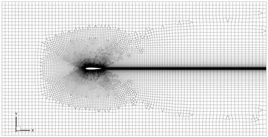
Figure 1.
Hybrid unstructured grid for NACA0012.
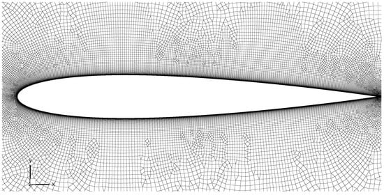
Figure 2.
Zoomed-in view.

Table 1.
Grid resolutions of previous DNS studies.
Due to the previously mentioned complex physics along the surface of aerofoil, an accurate representation of the near-wall structures is essential; therefore, a well-refined grid at the wall must be adopted. Here, the first cell height y is set to 0.00012 C, with an expansion rate of 1.1 for the following cells in the wall-normal direction; 150 cells are equally distributed in the span-wise direction, resulting in an averaged z = 0.0013 C. The averaged cell length in the stream-wise direction = 0.0036 C, where the minimum value is 0.0005 C at the leading edge and the trailing edge. The computed values for , , and along the upper surface of the aerofoil are plotted in Figure 3. Apart from a tiny portion of being slightly higher than 1 at near the leading edge, the overall value remains under 0.9 and approximately equals 0.5 in the separation region. The slightly excessive value does not affect the results []. The average value is less than 20 for most of the area and is below 9. The current wall resolutions are comparable to the wall-resolved LES determined by Asada and Kawai []. Piomelli and Balaras [] and Piomelli [] extensively discussed the grid requirements for wall-resolved LES; they estimated that grid resolution at the wall should be in the range of 50∽150 in the stream-wise direction, less than 2 in the wall-normal direction, and 15∽40 in the span-wise direction. The current wall resolutions should be considered sufficiently fine, and these parameters are displayed in Table 2 with high-fidelity references. It is also worth mentioning that the total number of cells is far less than that of DNS references [,,] since the current numerical framework (LES) does not fully resolve all the scales of motion of the field, and the grid cells are much coarser in the laminar region away from the aerofoil surface.
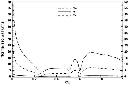
Figure 3.
The grid resolutions at the wall along the upper surface of the aerofoil.
Table 2.
The grid resolutions at the wall (averaged) and time-step comparison with high-fidelity references.
3.2. Boundary Conditions and Flow Initialization
The free stream Mach number 0.1 corresponds to a velocity magnitude of 34.3 m/s. The aerofoil is inclined at 4 degrees, resulting in a velocity vector of . A fixed-inlet boundary condition is imposed at the inlet and a convective boundary condition is applied at the outlet. A non-slip condition is applied at the aerofoil surface. The Neumann condition (zero-pressure gradient) is used for the pressure at the inlet and the aerofoil surface, while at the outlet, the pressure value is fixed at 0. Finally, a periodic boundary condition is applied for faces in the span-wise direction. A steady-state RANS simulation with a Spalart–Allmaras turbulence model is run for 500 iterations to obtain a more converged initial field, as it also helps reduce the time needed to obtain statistically converged results for later analysis []. From the initialized field, LES is run for a period of time units , corresponding to a physical time of 0.7 s. The time-step of s is defined to capture the Kolmogorove time scale, as discussed in the previous study []. The obtained CFL number is less than 1.5 in the boundary layer region. In total, 70,000 iterations are needed for 24; the data are collected and averaged for the last 12 after the initial transient period. The statical convergence is reached after 10.
4. Analysis and Discussion
4.1. Computational Cost
The details regarding computational cost are summarized in Table 3. A total of 128 CPUs were used for each simulation, half of those used for DNS case D []. The amount of CPU hours required to carry out the necessary simulation steps is significantly lower for current iLES and LES; however, the iLES based on the third-order WENO scheme is almost twice more expensive than the LES based on the WALE SGS model. It should be noted that approximately 3100 s was allocated to the calculation of the smooth indicator matrix for the WENO scheme and in addition to general storage. Additionally, the third-order WENO scheme requires an extra 400 G for storing matrix coefficients in order to accelerate the reconstruction process []. Thus, the third-order WENO-based iLES is generally more expensive than the WALE-based conventional LES.
Table 3.
Computational time.
4.2. Mean Pressure Distribution and Skin Friction Along Surface
The distribution of the mean pressure coefficient along the aerofoil surface is displayed in Figure 4, including the DNS data from Shan et al. [] and Smith and Ventikos []. From the leading edge to approximately x/C = 0.2, the pressure gradually increases towards the downstream direction, generating an adverse pressure gradient (∂p/∂x > 0), which causes the boundary layer to separate from the upper surface. A flattened plateau (0.3 < x/C < 0.53) denotes the laminar region of the separation zone, followed by a stronger second adverse pressure gradient (∂p/∂x > 0), where the separated boundary layer undergoes a transition to turbulence (0.53 < x/C < 0.6). The current observations are found to be similar to the flat plate case [,] and consistent with other LES investigations on aerofoil [,,]. A noticeable variation in mean values obtained in different averaging periods () can be observed in the laminar separation zone (0.2 < x/C < 0.65), revealing that the size of the separation bubble is related to the simulation time. Overall, the mean pressure coefficients ( = 24) from the current iLES and LES are in good agreement with the DNS presented by Smith [], while in the transitional and turbulent region (0.55 < x/C < 0.65), the iLES predicted a more consistent pressure distribution. However, evident disagreement is found when comparing these results to the DNS presented by Shan et al. []. The pressure increased faster downstream of the leading edge, and a much greater “bump” appeared in the transition zone; then, an under-predicted pressure was predicted near the trailing edge zone.
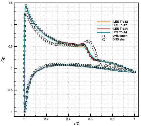
Figure 4.
Mean pressure coefficients obtained by LES and implicit LES, comparing with DNS from Shan et al. [] and Smith et al. []. = 12 denotes the normalized time when vortex shedding stabilized.
Skin friction has been assessed in many previous studies as an indicator of flow status; for instance, vanishing wall shear stress is the result of flow separation. The current mean values are plotted in Figure 5 and compared with the DNS results from Shan et al. []. The mean separation zone is estimated by zero crossings of the mean skin friction coefficient with a length of 0.36 C, where the mean separation location and mean re-attachment locations lie approximately at x = 0.24 C and x = 0.60 C, respectively. The current re-attachment location for LES and iLES is very close to that of the DNS from Smith [], who predicted a mean re-attachment at x = 0.56 C; however, according to the DNS results of Shan et al. [], the flow re-attached at a further downstream location, x = 0.68 C, and a much longer separation bubble with a length of 0.49 C was obtained. It was pointed out that the size of the separation bubble is related to time because of the large-scale oscillations in the three-dimensional flow []. Note that the simulations were run for a duration of 24 time units and 30 time units for both Smith [] and Shan et al. []; thus, the reason for the disagreement should exclude time convergence. It is worth mentioning that the negative skin coefficients in the plots indicating the boundary-layer separation and should always remain negative until the re-attachment further downstream.
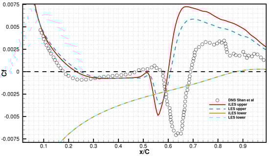
Figure 5.
Mean skin friction coefficients obtained by LES and implicit LES on upper and lower surface of the aerofoil. DNS data extracted from Shan et al. []. Note that the sign of values on the lower surface are intentionally reversed.
At around x = 0.5 C, a slight recovery followed by a negative surge immediately occurred, indicating the onset of a transition which agrees qualitatively with that from Spalart and Strelets [] and Alam and Sandham []. On the other hand, a recovery to positive values was obtained by Shan et al. [] in the middle of the separation zone, due to an additional thin layer of the mean flow near the wall in the stream-wise direction under the reversed flow. The accurate representation of the boundary-layer development is therefore in doubt as this thin layer was not observed in various other high-fidelity simulations, either [,,,,]. At location x = 0.58 C, a negative peak was reached by the current simulations; then, they recovered towards a positive value rapidly, indicating the end of the laminar transition to the turbulent boundary layer. After the re-attachment at x = 0.6 C, the skin friction coefficient continued to increase to a higher positive value quickly, then gradually dropping down. The DNS from Shan et al. [] showed a similar trend, apart from a largely delayed transition, re-attachment, and an “oscillated” post-attachment. On the lower surface, the computed skin friction coefficients are non-distinguishable from those of the current iLES and LES; additionally, the flow remains laminar and attached for most of the cord length. The separation occurs at a location near the trailing edge, which is explored in a later section.
4.3. Mean Velocity, Turbulent Stress Profiles, and Flow Field
The time-averaged stream-wise velocity field and its fluctuation field in the mid-span are illustrated in Figure 6 and Figure 7, respectively, and both fields were obtained through the iLES approach. At the leading edge, a small separation zone can be observed. As the fluid particle hits at the solid wall, it bounces backwards and is then pushed by the following stream-wise particle, thus naturally forming a small re-circling flow zone at the leading-edge area. Downstream of the leading edge, a long and thin region with considerable reversed flow is formed due to the separation and re-attachment of the boundary layer, which occur approximately at x = 0.2 C and x = 0.6 C, respectively, where the skin friction coefficients are zero, as seen in Figure 5. The thickness of the separation bubble gradually increases and reaches its maximum at around 75% of the total bubble length. The mean stream-wise fluctuation remains low and isotropic in the attached laminar region and most of the separated region; then, it increases quickly, where the separation bubble becomes the thickest and the peak value is clustered around the re-attachment location of the boundary layer. After the re-attachment, the mean stream-wise velocity in the near-wall region (y < 0.05 C) recovers a magnitude of 50% of the free stream and stays attached until it sweeps off the aerofoil surface into the wake. Meanwhile, the mean fluctuation gradually decreases but remains at a greater magnitude than that of the attached region. On the lower surface of the aerofoil, the flow is always attached, apart from a smaller reversed-flow region near the trailing edge, corresponding the zero crossing of the skin friction coefficient in Figure 5.
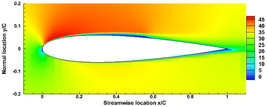
Figure 6.
Mean stream-wise velocity field.
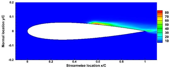
Figure 7.
Mean stream-wise fluctuation field.
Figure 8 shows an enlarged view of the mean separation region, demonstrated by the time-averaged velocity vector field. One can observe that the mean separation is located around x = 0.23 C, where the inflection point close to the wall is found. The reversed flow becomes stronger gradually downstream of the separation bubble. A second inflection point appears at around x = 0.6 C, indicating the re-attachment of the boundary layer. Note that at the location 0.05 C upstream of the re-attachment, the reversed flow is the strongest then quickly compromised. After the re-attachment, the mean velocity field is established within a short distance and the magnitude is amplified compared to that post-separation. It should be noted that the mean velocity vector plot from Shan et al. [] shows an additional thin layer underneath the reversed mean flow and, this thin layer forms approximately 22% of the total separation region. It is worth mentioning that their predicted mean separation length is 0.5 C, which is 0.14 C longer than that of the current simulation and similar to the length of that additional thin layer. As shown in Figure 4, the mean separation and re-attachment predicted by the current simulation is supported by the DNS recently reported by Smith []. The disagreement could be allocated to the insufficient span-wise extent to accommodate major scales of motion in the span direction, since an extent of 0.1 C was used by Shan et al. [], while at least 0.2 C was employed in other similar DNS studies [,,] where no such additional layer was identified.
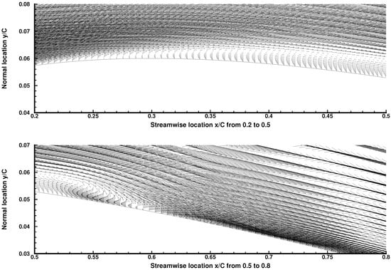
Figure 8.
Primary separation bubble on the upper surface, demonstrated by the mean stream-wise velocity vector field.
To further validate current numerical method and obtain more details on the averaged field, mean velocity profiles and root mean squared fluctuations are extracted at consecutive locations with an interval of 0.1 C from the leading edge to the tailing edge of the aerofoil.
Figure 9 shows mean stream-wise velocity profiles. The vertical distance from the wall is converted to a dimensionless form to remain consistent with the two main DNS references [,]. Compared to the DNS from Smith [] (figure on the left), discrepancies are clearly found at locations from x = 0.2 C to x = 0.6 C, corresponding with the separation zone. Since the wall is considered to be resolved, the disagreement with the DNS is mainly outside the viscous layer ( 10) for both the iLES and LES approaches; therefore, a better grid refinement to cover the entire separation zone seems to be necessary. It should be noted that the current expansion ratio of the wall-normal grid is set to 1.1, which could be considerably reduced to a smaller value. Despite this, the fully turbulent velocity profiles post re-attachment at locations x = 0.7 C, 0.8 C, 0.9 C, and 1 C are in excellent agreement with the DNS []. It is worth pointing out that at the re-attachment location x = 0.6 C, the profile determined by the LES approach is in better agreement than that by iLES. Compared to the DNS from Shan et al. [] (figure on the right), a good agreement is found at locations x = 0.2 C and x = 0.3 C, where the boundary is just separating from the surface. However, the disagreement appears in the rest of the locations. The mean velocity profiles predicted by Shan et al. [] after location x = 0.6 are not fully re-established, although they resemble the turbulent velocity profile. This is partially due to the additional thin layer which delayed re-attachment, thus forming a longer separation zone that occupies half of the chord length, possibly not providing sufficient lengths for the flow to be re-established []. It should also be noted that inflection points are observed, agreeing with Yang et al. []; an inflection point is the necessary and sufficient condition for flow to be inviscidly unstable.
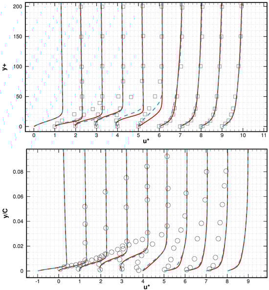
Figure 9.
Mean stream-wise velocity profiles compared with those from Smith [] (top, denoted in square) and Shan et al. [] (bottom, denoted in circle); from left to right: location at x/C = 0.1, 0.2, 0.3, 0.4, 0.5, 0.6, 0.7, 0.8, 0.9, 1. The solid red line denotes the iLES and the discontinued blue line denotes the LES.
Figure 10 shows an enlarged view of the separation zone, where the mean stream-wise velocity profiles are gathered at one location. It can be seen that not only the thickness of the separation bubble increases towards the downstream direction, but the amount of reversed flow also increases. At each location, the amount of reversed flow has a small difference between the current simulations and the DNS, but a major difference is found in the wall-normal direction. For instance, at location x = 0.5 C, the reversed flow is about 6% of the free-stream velocity and is located at = 5 for iLES, 6.5% at = 6 for LES, and 6.1% at = 15 for DNS. Here, this difference seems to have little impact on the flow development at a later stage, as the re-attached turbulent boundary layer is captured with excellent agreement. The maximum reversed flow of 12% is found at x = 0.55 C in the current simulations (not displayed in the figure and similar to the DNS from Smith []), while in the DNS from Shan et al. [], 26% was found at x = 0.6 C. Alam and Sandham [] concluded that velocity profiles with more than 15% reversed flow are required for absolute stability (disturbances grow in time), while less than 15% is considered convective stability (disturbances grow in space). This condition is not met by the current simulations. Hence, it can be assumed that the current separation bubble has a similar behavior to that from Alam [] and Yang [], where an inviscidly instability is triggered by the Kelvin–Helmholtz mechanism.
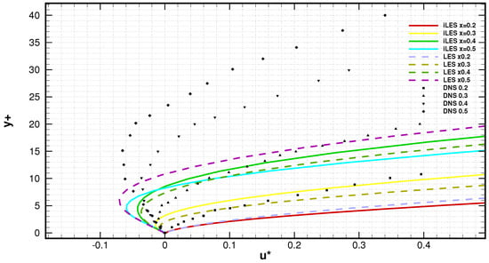
Figure 10.
Enlarged view of mean stream-wise velocity profiles at locations x/C = 0.2, 0.3, 0.4, and 0.5, where the separation takes place.
The mean transverse and span-wise velocity profiles are displayed in Figure 11 and Figure 12 respectively. Similar patterns are captured by both iLES and LES approaches for mean transverse profiles, the main difference can be identified at locations x = 0.5 C, 0.6 C and 0.7 C, corresponding the re-attachment area. At the location near leading edge, the transverse velocity has been amplified to 350% of its free-stream magnitude then slowly been reduced until its lowest at location x = 0.4 C, right in the middle of the separation bubble. At locations closer to the re-attachment area, the transverse velocity has changed its direction fast towards the wall, then remains at about −110% after the re-attachment. The transverse profiles are quite similar to turbulent stream-wise profiles, but with an opposite direction. By examining the span-wise profiles in Figure 12, the flow is found dominated by two-dimensional motions at initial stage, as the mean span-wise velocity remains constant until x = 0.5 C, where a variation is observed, indicating the rise of three-dimensionality. The span-wise variation emerges firstly in viscous layer () then propagates upwards from the wall. At locations after x = 0.5 C, the profiles remain oscillated, highlighting the strong three-dimensional motion of the flow.
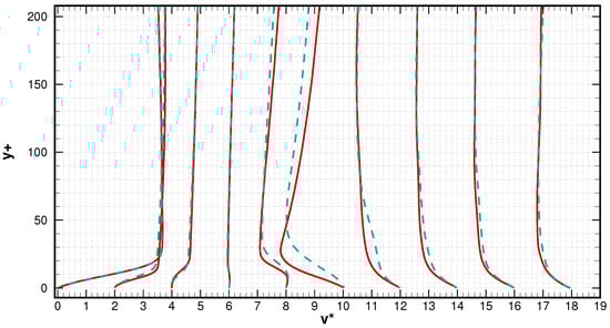
Figure 11.
Mean transverse velocity profiles, from left to right are location at x/C = 0.1, 0.2, 0.3, 0.4, 0.5, 0.6, 0.7, 0.8, 0.9, 1. The solid red line denotes iLES and the discontinued blue line denotes the LES.
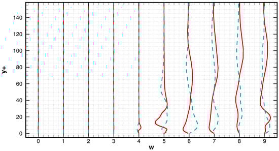
Figure 12.
Mean span-wise velocity profiles, from left to right are location at x/C = 0.1, 0.2, 0.3, 0.4, 0.5, 0.6, 0.7, 0.8, 0.9, 1. The solid red line denotes iLES and the discontinued blue line denotes the LES.
The root mean squared stream-wise and transverse fluctuations are plotted in Figure 13 and Figure 14. These quantities are strongly related to the turbulence level of flow. At a short distance from the separation point, the flow is still laminar as no fluctuation appears in the stream-wise and transverse directions. From location x = 0.5 C to x = 0.6 C, fluctuations are suddenly intensified near the wall, and a transition to turbulence is believed to occur after the instability emerges in the separating boundary layer. The transition is also reflected by the strong gradient in the plots of the pressure coefficients seen in Figure 4 and the skin friction coefficients in Figure 5. The stream-wise fluctuation peaks are at a wall distance of 7 at x = 0.6 C for both the iLES and LES approaches, but the former decreases much faster as it distances itself from the wall. Additionally, the transverse fluctuation peak is at 15 for theiLES, while for the LES, the peak is higher, at 30. In other words, the iLES predicted a higher fluctuation in the near-wall area at the re-attachment region (x ≈ 0.6). The strongest fluctuation is found around the transition re-attachment area, similar to that found by Sato et al. []. When the flow was re-established, both approaches predicted non-distinguishable fluctuation profiles. The R.M.S of the kinetic energy is shown in Figure 15, and data from Smith [] are also included. Apart from the re-attachment area (x = 0.6 C), the profiles are within satisfactory agreement with the DNS reference, where the flow remains smooth in the first half of the separation zone and is then governed by strong turbulent activities from the re-attachment area to the tailing edge. It should be noted that the profile obtained by the LES approach is closer to that of the DNS reference than the iLES at the re-attachment area, possibly suggesting an insufficient dissipation in the viscous layer for the latter approach.
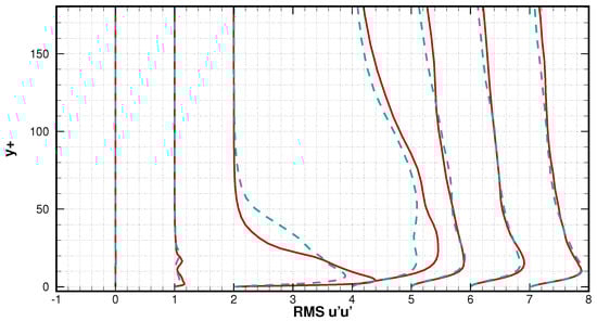
Figure 13.
Root mean square of stream-wise velocity fluctuation profiles; from left to right: locations at x/C = 0.4, 0.5, 0.6, 0.7, 0.8, 0.9, 1. The solid red line denotes the iLES and the discontinued blue line denotes the LES.
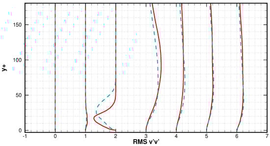
Figure 14.
Root mean square of transverse velocity fluctuation profiles; from left to right: locations at x/C = 0.4, 0.5, 0.6, 0.7, 0.8, 0.9, 1. The solid red line denotes iLES and the discontinued blue line denotes the LES.
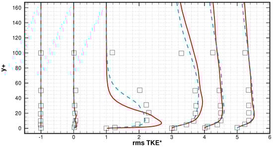
Figure 15.
Root mean square of TKE profiles compared with those from Smith []; from left to right: locations at x/C = 0.4, 0.5, 0.6, 0.7, 0.8, 0.9. The solid red line denotes iLES and the discontinued blue line denotes the LES.
Finally, an overall physical phenomenon can be summarized based on the time-averaged field as follows: The laminar boundary layer is formed after the flow passes the leading edge of the aerofoil surface. Due to the adverse pressure gradient and curvature of the surface, the boundary layer separates at around x = 0.23 C. The separating boundary layer remains laminar for more than half of its total length then undergoes a transition to turbulent between x = 0.5 and x = 0.6, resulting in a fast negative surge of the skin friction coefficient and rapidly intensified turbulent fluctuations. The re-attachment takes place at around 0.6C, thus forming a separation bubble. The turbulent boundary layer is then established quickly and stays attached to the surface until it finally sweeps off into the wake. Span-wise variation occurs before the transition to turbulence, and it is located at about half of the mean bubble length; the flow becomes three-dimensional and then turbulent. The whole process shares similarities with that presented by Yang et al. [], where the flow is past the curvature-induced plate. Currently, both the iLES and LES show good reliability in a time-averaged flow.
4.4. Boundary Layer Development
In this section, the instantaneous flow field obtained by the iLES is discussed to further asses the numerical approach and explore more flow characteristics.
4.4.1. Instantaneous Flow Structure
Figure 16 shows the evolution of the boundary layer from the initial stage. The sub-figures on the left represent the iso-surfaces of the Q-criterion colored by the instantaneous stream-wise velocity, while on the right, the vorticity magnitude at the mid-span is illustrated. At the beginning, a long and smooth layer which covers the first half the cord denotes the laminar boundary layer. It rolls up and separates from the surface at around the middle cord location due to the Kelvin–Helmholtz instability mechanism. Large-scale vortex shedding can be observed; they are two-dimensional and turn around the span-wise axis. At the next time interval, disturbance is found near the trailing edge, where the large-scale vortices tend to lose their shapes as a result. Meanwhile, smaller vortices are formed in the boundary layer separation zone. Next, the large-scale vortices near the trailing edge break down into smaller vortices and are joined by small vortices which are convecting from the upstream. At the following time-step, vortices formed by the boundary layer roll-up quickly break down into hairpin-like structures and become three-dimensional as the flow convects downstream. Here, Yang and Voke [] and Roshko [] pointed out that the span-wise length of two ends of the hairpin vortices is about the same as a Kelvin–Helmholtz wavelength, indicating that the transition from two-dimensional to three-dimensional is mainly triggered by the –Helmholtz instability. As the fluctuation propagates downstream, the vortices speed up and break into smaller ones and become fully turbulent quickly, just before the re-attachment.
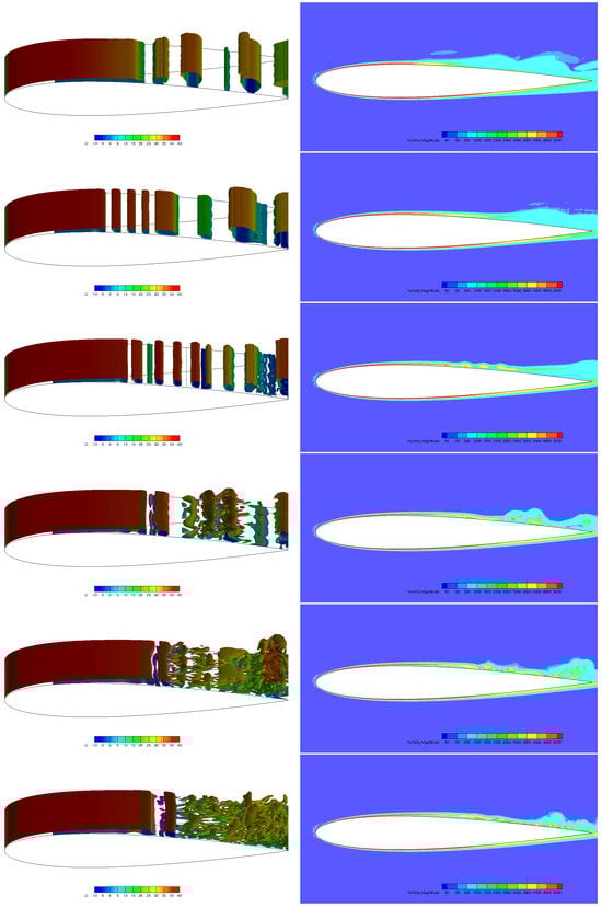
Figure 16.
Snapshots showing the early development of the boundary layer, top to bottom images are displayed in the order of dimensionless time of 0.34, 0.68, 1.02, 1.36, 1.7, and 2.04.
Finally, the irregular vortex shedding is established, involving laminar separation, vortex breakdown and transition to turbulence, and re-attachment to the surface, as can be clearly observed in Figure 17. Recall that the mean turbulent kinetic energy reaches its maximum at around 60% of the chord length (Figure 15), corresponding to the location where the transition to turbulence takes place. This is in agreement with the current vortex visualization. The whole process is found to be qualitatively consistent with that from Spalart and Strelets [] and Jones et al. [], further validating the suitability of the current iLES on predicting flow with complexity. A failed example of LES is demonstrated in Smith []; the Smagorinsky SGS model was not able to capture the transition for three levels of grid (due to excessive dissipation); therefore, the predicted boundary layer remains laminar on both sides of the aerofoil, while the dynamic k model captured the transition reasonably. This proves that an accurate representation of the SGS effect is a key factor to resolve the transition. In addition, Asada and Kawai [] stressed that it is essential to resolve the transition in order to accurately capture the flow physics such as the skin friction and turbulent boundary layer further downstream.
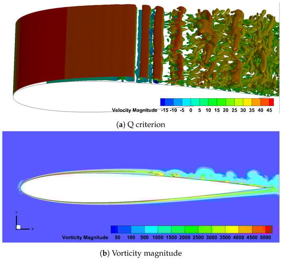
Figure 17.
The boundary layer at dimensionless T* = 24, the last time step of simulation.
It should be noted that the length and shape of the separation bubble are constantly changing, even after the flow is established; a consecutive time series of snapshots of an enlarged view of the separation bubble are illustrated in Figure 18. As one can observe on the figures on the top and bottom, only one long bubble appears, and the greater the amount of instantaneous reversed flow, the further downstream the re-attachment location is; thus, the separation bubble is longer. The figures in the middle demonstrate a separation zone made up of several consecutive small bubbles, and the separation and re-attachment take place multiple times. The first re-attachment can be observed at as early as 47% of the cord length and as late as 64% (note that the mean re-attachment location is around 60%). Therefore, it can be concluded that the formation of the separation bubble is irregular and highly time-dependant. Similarly, on the curved plate, Yang and Voke [] showed that the variation in the instantaneous re-attachment location can be up to 50% of the mean re-attachment.
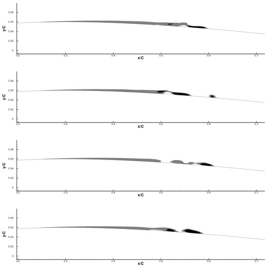
Figure 18.
Snapshots of the primary separation bubble on the suction side.
4.4.2. Velocity Spectra and Time-Series
Spectral analysis is necessary to reveal more insights into this highly unsteady flow. To monitor the transition process during the course of simulation, probes (as described in Table 4) are placed along the aerofoil at the fourth cell to the wall, which is inside of the viscous layer of the boundary layer. At each probe, stream-wise and transverse velocities are evenly sampled for every time-step of s, and a total of 35,000 samples were collected. Similarly, the Hann window is used to perform FFT to obtain the velocity spectra.
Table 4.
Probe locations in mid-span, at the same cord-wise location where the velocity profiles were extracted previously.
The spectra for the stream-wise and transverse velocity components are displayed in Figure 19. At 20% of the chord length, where the separation is about to take place, the linearly decreased spectra show a purely laminar flow feature. A peak can be observed at around 300 Hz at 30% of the chord length, corresponding to a shedding frequency of the laminar flow separating the boundary layer. This peak is then sharply amplified at 40% of the chord length due to the convective instability; note that at a higher frequency range, the smaller scales are still in the same order of magnitude as the upstream locations, indicating that the amplification is only applied to the larger vortices. It should be also taken into account that the span-wise disturbance begins to emerge, as shown in Figure 12. At half of the length of the cord, all scales have an oscillation amplitude at least one order of magnitude higher, the narrow band peak and its second harmonic are very pronounced, and the transition to turbulence is on course to take place. Note that the transition is mostly triggered by upstream disturbances or a change in surface roughness; however, the transition in the current context seems to be self-induced, without external influence. Similarly, Spalart and Strelets [] demonstrated a transition that was independent of incoming disturbances.
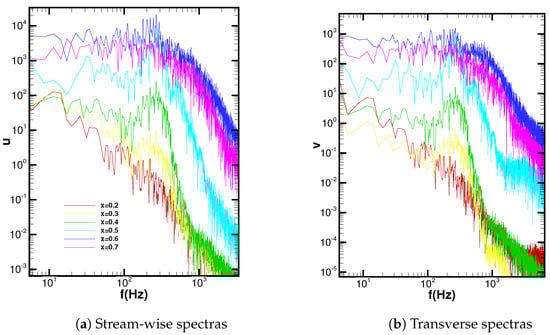
Figure 19.
Velocity spectra at locations (from bottom to top) x = 0.2 C, 0.3 C, 0.4 C, 0.5 C, 0.6 C, and 0.7 C.
Shan et al. [] pointed out a possible original source of the three-dimensional disturbance which propagates upstream from the trailing edge that triggers the transition. As the boundary layer re-attaches to the surface at around 60% of the cord length, the narrow band peak becomes much less pronounced and tends to disappear as the fully turbulent flow is established. This is because of the breakdown of larger scales in the transition process and because more, smaller scales amplified with turbulent kinetic energy are created at a high range of frequency. Figure 15 confirms that the turbulent kinetic energy reached the highest level at this location. In addition, a similar magnitude of amplitude is found in both stream-wise and transverse directions at higher frequency ( Hz), revealing the isotropic feature of small scales of the fully turbulent boundary layer. The above observations on the velocity spectra are in good agreement with the DNS study by Smith and Ventikos [], where the initial disturbance, which is also characterized by a peak, is found to grow rapidly between 0.4 C and 0.5 C. A flattened spectrum denotes the fully turbulent status of the boundary layer after re-attachment.
In addition to velocity spectra, the entire time histories of stream-wise velocity are recorded and displayed in Figure 20. The dashed lines from the beginning to dimensionless time = 12 are excluded to obtain a time-averaged flow field, as the initial numerical transients can be clearly observed. For the first half of the cord length, the velocity magnitude is always smooth and gradually decreases to a negative value, corresponding to the laminar separation. Particular attention is paid to the middle of cord; after a period of numerical transition ( 3), the velocity oscillation magnitude becomes significantly amplified with time, until 13, and then suddenly decreases but still remains higher than its initial level in later time series. From the visualization shown in Figure 16, it is known that at the location where x = 0.5 C, the vortices which are forming by the roll-up of the laminar boundary layer break down with the rise in three-dimensionality, and a transition to turbulence occurs. It could be speculated that disturbance is gathered from multiple sources at the middle of cord as the transition process continues and the breakdown is accelerated, until a balance of small vortex production and shading is established.
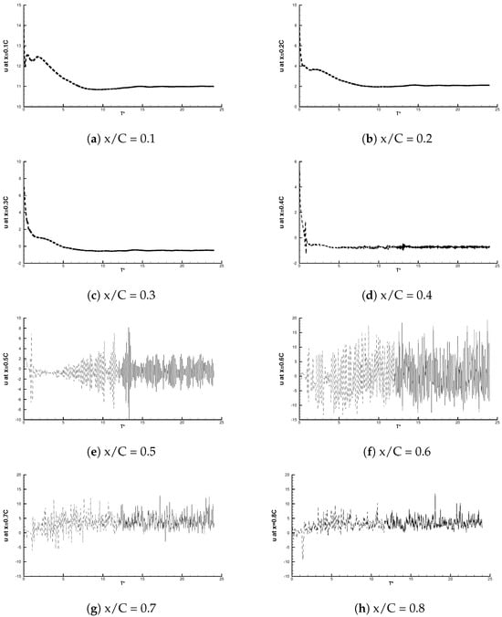
Figure 20.
Full time history of stream-wise velocities at various locations near the wall on the upper surface of the aerofoil.
The velocity had the highest oscillation amplitude at x = 0.6 C, as expected, and then gradually increased as the turbulent kinetic energy dissipated at downstream locations. In the current investigation, no evidence has been found yet to identify the original source of the disturbance, in addition to Kelvin–Helmholtz instability, which is mainly responsible for the formation of three-dimensionality. The DNS study by Shan et al. [] suggested a disturbance at the wake after analysing the time histories of stream-wise velocity, but the conclusion was obtained without analysing the detailed flow structure and the cause of the disturbance remains unclear. Thus, in the following, the trailing edge dynamics are explored.
4.4.3. The Separation Bubble near the Trailing Edge
An enlarged view of the mean separation zone near the trailing edge is shown in Figure 21. The higher density of the vector fields on the upper surface of the aerofoil can be seen, and even after sweeping off, its boundary is still aligned with the upper surface and joined by the reversed flow from downstream of the trailing edge. Another part of the reversed flow moves further upstream at the lower surface, forming a significant reversed zone. The boundary layer on the lower surface remains attached and laminar from the leading edge until it is countered by this reversed flow, which separates it from the surface. Note in the Figure 5, the zero crossing of the lower surface skin coefficients near the tailing edge reflect the separation. Before joining the wake, the inner part of the separated free shear layer is “sucked” back, with one big part rejoining the reserved flow zone and another smaller part becoming absorbed by the turbulent free shear layer on the upper part. Here, two vortices can be identified near the trailing edge. From the time-averaged vector field, it can be concluded that these two vortical structures are self-sustained, and the process of their creation can be revealed by analysing the evolution of the flow near the trailing edge from the initial stage.
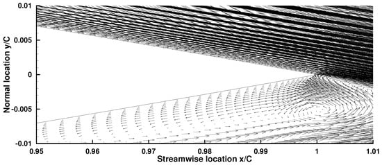
Figure 21.
Mean reversed flow zone near trailing edge.
Similar to Figure 16, the initial development of the trailing edge separation bubble at consecutive time steps is shown in Figure 22. The instantaneous stream-traces are demonstrated and the background is coloured by the stream-wise velocity, where the red and green denote the region with stream-wise direction. In the top figure, at a distance upstream of the trailing edge, a large energetic vortex is observed. At this stage, the flow on the upper surface downstream of the large vortex seems to have less kinetic energy and is drawn by the flow on the lower side at the trailing edge; a minor disturbance can be seen immediately. In the next moment, the vortex arrives at the trailing edge and is amplified by a large portion of the flow on the lower side, forming a large instantaneous separation bubble and causing greater distortion of the flow near the trailing edge.
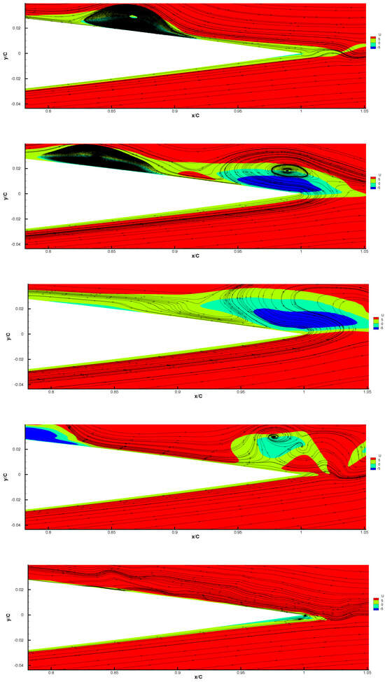
Figure 22.
Initial development of vortex shedding near trailing edge.
In the following figures, it can be observed that the bubble has further increased in size due to the amplification of the vortex from upstream and the flow on the lower surface. On the side of the large vortex, a secondary vortex is formed, corresponding to the appearance of span-wise structures at the same time step in Figure 16, where the instability emerges. Next, the large vortex breaks up into smaller ones and injects more kinetic energy into the upper flow field. Note that the flow stream trace on the lower side bends upwards. It is worth mentioning that at the same time, hairpin structures emerge near the re-attachment zone, indicating that the increase in three-dimensionality upstream appears slightly later than that near trailing edge. As shown in the last figure, the motion of flow on the upper side is represented by the fluctuated stream-traces and remains attached. On the other hand, a clear separation zone can be found on the lower side and two vortical structures are identified inside, as a result of the intersection of turbulent and laminar flow on the upper and lower sides.
The stream-wise velocity time history from additional probes which are located on the upper and lower surfaces of the aerofoil near the trailing edge are displayed. Figure 23 shows the locations upstream of the trailing edge; the red line represents the upper side and the green line represents the lower side. At locations x = 0.8 C and x = 0.9 C, the upper side velocities share the same pattern at the initial stage, with an average magnitude less than 0, confirming that the separation bubble appears alternatively, as shown in the visualization (see Figure 16 and Figure 22). After the transient period ( 2), the velocities fluctuate around a mean magnitude bigger than zero, indicating an attached and turbulent flow. An obvious difference can be observed for the velocities on the lower side, as the flow remains laminar and there is no fluctuation even at the transient stage.
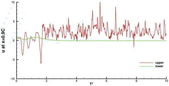
Figure 23.
Stream-wise velocity histories at x/C = 0.9. The red line denotes the velocity recorded by the probe on the upper surface and the green line represents the lower surface.
At the location x = 0.99 C, the lower velocities show a similar transient fluctuation pattern to the upper velocities, and the fluctuation magnitude is greatly decreased and stabilized around a mean value smaller than 0. This confirms that a small reversed flow region is formed, co-related to the upper velocities. Figure 24 shows two locations downstream of the trailing edge; the oscillation amplitude becomes greater as the flow moves further into the wake. However, there is no obvious disturbance found related to time. It can be concluded that the disturbance near the trailing edge is the consequence of an interaction between the seeping turbulent boundary layer from the upper side and the laminar boundary layer from the lower side. The resulting bubble at the trailing edge bursts, introducing span-wise distortion which propagates upstream. However, three-dimensional perturbation caused by numerical residual fluctuation [] cannot be not ruled out.
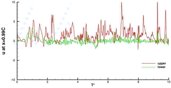
Figure 24.
Stream-wise velocity histories at x/C = 0.99. The red line denotes the velocity recorded by the probe on the upper surface and the green line represents the lower surface.
5. Conclusions
iLES and LES investigations were carried out on the separated flow around the NACA0012 aerofoil, at an incidence of 4 degrees and with a moderate Reynolds number of . The total number of finite volume cells was kept as low as , of the grid used in the DNS of Smith [] and much less than most of the LES in the literature. To validate the fidelity of the current numerical approach, results were compared with two DNS studies [,] which were conducted under the same flow configurations.
The mean lift and drag coefficients are indistinguishable between iLES and LES, and the variance is found to be within 10% compared to the experimental data from the closest flow configuration. The mean surface pressure coefficients are in excellent agreement with the DNS of Smith [], and the iLES gives a better prediction in the separated transitional region. The mean re-attachment is located at around x = 0.6 C for iLES and LES, in close agreement with Smith [], who predicted x = 0.56 C, and coincides with the boundary layer transition region. The mean velocity profiles showed a fully established turbulent boundary layer after re-attachment, accurately matching with the DNS of Smith []. However, it should be noted that in the separation zone, the current profiles are distinct from the profiles of Smith [] at a normal wall distance higher than = 10, although the amount of reversed flow is in satisfactory agreement. Further, at the re-attachment location x = 0.6 C, the mean r.m.s of fluctuations predicted by LES has a better agreement with DNS than iLES.
It is worth noting that for such a separated transitional flow, even if all scales of motions are considered resolved, a large discrepancy can still be found on the mean flow field between the DNS of Shan et al. [] and Smith []. In the author’s opinion, the DNS of Smith [] should be more reliable due to following reasons: it has a much bigger computational domain and a larger number of total finite volume cells; there is a fully three-dimensional simulation; and the current results and other LES studies [,,] are in qualitatively agreement and consistent with Smith [] regarding the mean pressure coefficient along the aerofoil surface.
The instantaneous flow field can be obtained using the iLES approach, where the entire physical process on the upper surface of the aerofoil is captured. The process involves laminar boundary layer separation, the formation of a large scale vortex, a rise in three-dimensionality, vortex breakdown and transition to turbulence, re-attachment and the establishment of a fully turbulent boundary layer. The shape and length of the formed separation bubble changes instantaneously, as the locations of separation and re-attachment are not fixed. On the lower part of the aerofoil, the boundary layer remains laminar and attached until 90%, and then separates due to a stronger reversed flow from the lower part of the near wake. The spectral analysis demonstrated the validity of the predicted instantaneous flow evolution through a comparison with the DNS of Smith []. For the physical perspective, the first instability is induced via a Kelvin–Helmholtz mechanism, followed by a second instability which gives rise to the three-dimensionality. The span-wise disturbance is found to be related to the vortex breakdown, and leads to the transition to turbulence. Here, a reversed flow with a maximum amount of 12% free stream magnitude is found, suggesting a convective instability, in agreement with Jones et al. []. Shan et al. [] pointed out that the span-wise instability first emerges in the near wake; following this suggestion, the dynamics of the near wake were explored. A possible cause of the disturbance is attributed to the interaction of two separating free shear layers at the early stage.
The current iLES approach, based on a third-order WENO scheme [], is capable of dealing with wall-bounded flow involving separation and transition. Although only a second-order overall accuracy is achieved, the computed mean quantities such as surface pressure coefficient, turbulent velocity profiles and turbulent kinetic energy profiles are in satisfactory agreement with the DNS reference. Note that despite the current prediction of the near-wall velocity profiles being different in the separation zone (Figure 9 and Figure 10, hence a thinner separation bubble), the fully turbulent boundary layer at the re-attachment zone is still captured with excellent agreement. It has been proven that the near-wall resolution is essential to accurately predict such a complex flow. To overcome the current weakness, it is recommended to increase near-wall resolution by reducing the wall’s normal expansion ratio in the separation zone only. Also, the excessive turbulent kinetic energy is predicted by iLES at the very near wall, indicating the possible lack of dissipation in the near-wall region.
Author Contributions
Conceptualization, Z.L.; methodology, Z.L. and Z.A.R.; software, Z.L.; validation, Z.L.; formal analysis, Z.L.; resources, Z.A.R.; writing—original draft preparation, Z.L.; writing—review and editing, Z.A.R.; visualization, Z.L.; project administration, Z.L. and Z.A.R. All authors have read and agreed to the published version of the manuscript.
Funding
This research received no external funding.
Data Availability Statement
The data and codes for the simulation will be available upon request to the authors.
Acknowledgments
This research has extensively employed the Cranfield University High Performance Computing (HPC) facility. The authors would like to acknowledge the support and guidance received from Mick Knaggs at the Cranfield HPC department.
Conflicts of Interest
The authors declare no conflicts of interest.
Abbreviations
| CFD | Computational Fluid Dynamics |
| LES | Large Eddy Simulation |
| RANS | Reynolds Average Navier–Stokes |
| PISO | Pressure-Implicit Splitting Operator |
| WENO | Weighted Essentially Non-Oscillatory |
| Kinematic viscosity (m2/s) | |
| Weight (-) | |
| Sub-Grid-Scale tensor | |
| SGS viscosity | |
| Filter width | |
| Reynolds number (-) | |
| p | Kinematic pressure (m2/s2) |
| Velocity vector (m/s) | |
| t | Time (s) |
| Time unit (s) | |
| V | Volume of a cell (m3) |
| SGS kinetic energy | |
| S | Area of a face (m2) |
| Span-wise extend lenth | |
| Surface flux (-) | |
| Normal unit vector of a surface | |
| Cartesian coordinates (m) | |
| Dimensionless distance | |
| U | Free-stream velocity (m/s) |
| C | Cord length of aerofoil (m3) |
| Velocity components | |
| Q | Q criterion |
| Flux | |
| Mach number | |
| Normal stress components | |
| Shear stress component | |
| Pressure coefficient (-) | |
| Lift coefficient (-) | |
| Drag coefficient (-) |
References
- Sakellariou, K.; Rana, Z.A.; Jenkins, K.W. Optimisation of the surfboard fin shape using computational fluid dynamics and genetic algorithms. Proc. Inst. Mech. Eng. Part P J. Sport. Eng. Technol. 2017, 231, 344–354. [Google Scholar] [CrossRef]
- Expósito, D.; Rana, Z.A. Computational investigations into heat transfer over a double wedge in hypersonic flows. Aerosp. Sci. Technol. 2019, 92, 839–846. [Google Scholar] [CrossRef]
- Bagul, P.; Rana, Z.A.; Jekins, K.W.; Konozsy, L. Computational engineering analysis of external geometrical modifications on MQ-1 unmanned combat aerial vehicle. Chin. J. Aeronaut. 2020, 33, 1154–1165. [Google Scholar] [CrossRef]
- Rodi, W. Comparison of LES and RANS calculations of the flow around bluff bodies. J. Wind. Eng. Ind. Aerodyn. 1997, 69–71, 55–75. [Google Scholar] [CrossRef]
- Rumsey, C.L.; Nishino, T. Numerical study comparing RANS and LES approaches on a circulation control airfoil. Int. J. Heat Fluid Flow 2011, 32, 847–864. [Google Scholar] [CrossRef]
- Zhang, Y.; van Zuijlen, A.; van Bussel, G. Massively separated turbulent flow simulation around non-rotating MEXICO blade by means of RANS and DDES approaches in OpenFOAM. In Proceedings of the 33rd AIAA Applied Aerodynamics Conference, Dallas, TX, USA, 22–26 June 2015; pp. 1–10. [Google Scholar] [CrossRef]
- Zhang, Y.; Deng, S.; Wang, X. RANS and DDES simulations of a horizontal-axis wind turbine under stalled flow condition using OpenFOAM. Energy 2018, 167, 1155–1163. [Google Scholar] [CrossRef]
- Spalart, P.R.; Strelets, M.K. Mechanisms of transition and heat transfer in a separation bubble. J. Fluid Mech. 2000, 403, 329–349. [Google Scholar] [CrossRef]
- Chapman, D. Computational Aerodynamics Development and Outlook. AIAA J. 1979, 17, 1293–1313. [Google Scholar] [CrossRef]
- Choi, H.; Moin, P. Grid-point requirements for large eddy simulation: Chapman’s estimates revisited. Phys. Fluids 2012, 24, 011702. [Google Scholar] [CrossRef]
- Drikakis, D.; Fureby, C.; Grinstein, F.F.; Youngs, D. Simulation of transition and turbulence decay in the Taylor-Green vortex. J. Turbul. 2007, 8, 1–12. [Google Scholar] [CrossRef]
- Grinstein, F.F.; Margolin, L.G.; Rider, W.J. Implicit Large Eddy Simulation: Computing Turbulent Fluid Dynamics; Cambridge University Press: Cambridge, UK, 2007. [Google Scholar] [CrossRef]
- Davidson, L.; Cokljat, D.; Frohlich, J.; Leschziner, M.A.; Mellen, C.; Rodi, W. LESFOIL: Large Eddy Simulation of Flow Around a High Lift Airfoil; Springer: Berlin/Heidelberg, Germany, 2003. [Google Scholar] [CrossRef]
- Smith, T.A.; Ventikos, Y. Boundary layer transition over a foil using direct numerical simulation and large eddy simulation. Phys. Fluids 2019, 31, 124102. [Google Scholar] [CrossRef]
- Boris, J.P. On large eddy simulation using subgrid turbulence models Comment. In Whither Turbulence? Or Turbulence at the Crossroads; Springer: Berlin/Heidelberg, Germany, 1990; pp. 344–353. [Google Scholar] [CrossRef]
- Beaudan, P.; Moin, P. Numerical Experiments on the Flow Past a Circular Cylinder at Sub-Critical Reynolds Number; Stanford University: Palo Alto, CA, USA, 1994; pp. 1–262. [Google Scholar]
- Breuer, M. Large eddy simulation of the subcritical flow past a circular cylinder: Numerical and modeling aspects. Int. J. Numer. Methods Fluids 1998, 28, 1281–1302. [Google Scholar] [CrossRef]
- Kravchenko, A.; Moin, P. Numerical simulation of flow over a circular cylinder at low Reynolds number. Phys. Fluids 2000, 12, 942–946. [Google Scholar] [CrossRef]
- Ouvrard, H.; Koobus, B.; Dervieux, A.; Salvetti, M.V. Classical and variational multiscale LES of the flow around a circular cylinder on unstructured grids. Comput. Fluids 2010, 39, 1083–1094. [Google Scholar] [CrossRef]
- Drikakis, D.; Rider, W. High-Resolution Methods for Incompressible and Low-Speed Flows; Springer: Berlin/Heidelberg, Germany, 2005. [Google Scholar] [CrossRef]
- Liu, X.D.; Osher, S.; Chan, T. Weighted Essentially Non-Oscillatory Schemes. J. Comput. Phys. 1994, 115, 200–212. [Google Scholar] [CrossRef]
- Hahn, M. Implicit Large-Eddy Simulation of Low-Speed Separated Flows Using High-Resolution Methods. Ph.D. Thesis, Cranfield University, Cranfield, UK, 2008. [Google Scholar]
- Dumbser, M.; Käser, M. Arbitrary high order non-oscillatory finite volume schemes on unstructured meshes for linear hyperbolic systems. J. Comput. Phys. 2007, 221, 693–723. [Google Scholar] [CrossRef]
- Tsoutsanis, P.; Titarev, V.A.; Drikakis, D. WENO schemes on arbitrary mixed-element unstructured meshes in three space dimensions. J. Comput. Phys. 2011, 230, 1585–1601. [Google Scholar] [CrossRef]
- Tsoutsanis, P.; Antoniadis, A.F.; Drikakis, D. WENO schemes on arbitrary unstructured meshes for laminar, transitional and turbulent flows. J. Comput. Phys. 2014, 256, 254–276. [Google Scholar] [CrossRef]
- Zeng, K.; Li, Z.; Rana, Z.A.; Jenkins, K.W. Implicit Large Eddy Simulations of Turbulent Flow around a Square Cylinder at Reynolds Number of 22,000. Comput. Fluids 2021, 226, 105000. [Google Scholar] [CrossRef]
- Martin, T.; Shevchuk, I. Implementation and Validation of Semi-Implicit WENO Schemes Using OpenFOAM®. Computation 2018, 6, 6. [Google Scholar] [CrossRef]
- Rad, S.H.; Ghafoorian, F.; Taraghi, M.; Moghimi, M.; Asl, F.G.; Mehrpooya, M. A systematic study on the aerodynamic performance enhancement in H-type Darrieus vertical axis wind turbines using vortex cavity layouts and deflectors. Phys. Fluids 2024, 36, 125170. [Google Scholar] [CrossRef]
- Mirmotahari, S.R.; Ghafoorian, F.; Mehrpooya, M.; Rad, S.H.; Taraghi, M.; Moghimi, M. A comprehensive investigation on Darrieus vertical axis wind turbine performance and self-starting capability improvement by implementing a novel semi-directional airfoil guide vane and rotor solidity. Phys. Fluids 2024, 36, 065151. [Google Scholar] [CrossRef]
- Lissaman, P.B.S. Low-reynolds-number airfoils. Annu. Rev. Fluid Mech. 1983, 223–239. [Google Scholar] [CrossRef]
- Jones, L.E.; Sandberg, R.D.; Sandham, N.D. Direct numerical simulations of forced and unforced separation bubbles on an airfoil at incidence. J. Fluid Mech. 2008, 602, 175–207. [Google Scholar] [CrossRef]
- Bertolotti, F.P.; Herbert, T.; Spalart, P.R. Linear and nonlinear stability of the blasius boundary layer. J. Fluid Mech. 1992, 242, 441–474. [Google Scholar] [CrossRef]
- Herbert, T. Parabolized stability equations. Annu. Rev. Fluid Mech. 1997, 29, 245–283. [Google Scholar] [CrossRef]
- Rodríguez, I.; Lehmkuhl, O.; Borrell, R.; Oliva, A. Direct numerical simulation of a NACA0012 in full stall. Int. J. Heat Fluid Flow 2013, 43, 194–203. [Google Scholar] [CrossRef]
- Shan, H.; Jiang, L.; Liu, C. Direct numerical simulation of flow separation around a NACA0012 airfoil. Comput. Fluids 2005, 34, 1096–1114. [Google Scholar] [CrossRef]
- Mellen, C.P.; Fröhlich, J.; Rodi, W. Lessons from the European LESFOIL project on LES of flow around an airfoil. In Proceedings of the 40th AIAA Aerospace Sciences Meeting and Exhibit, Reno, NV, USA, 14–17 January 2002. [Google Scholar] [CrossRef]
- Nicoud, F.; Ducros, F. Subgrid-Scale Stress Modelling Based on the Square of the Velocity Gradient Tensor. Flow Turbul. Combust. 1999, 62, 183–200. [Google Scholar] [CrossRef]
- Moukalled, F.; Mangani, L.; Darwish, M. The Finite Volume Method in Computational Fluid Dynamics; Springer: Berlin/Heidelberg, Germany, 2016; Volume 113, pp. 535–557. [Google Scholar] [CrossRef]
- Jasak, H. Error Analysis and Estimation for the Finite Volume Method with Applications to Fluid Flows. Ph.D. Thesis, Imperial College London, London, UK, 1996. [Google Scholar]
- Cao, Y.; Tamura, T. Large-eddy simulations of flow past a square cylinder using structured and unstructured grids. Comput. Fluids 2016, 137, 36–54. [Google Scholar] [CrossRef]
- Warming, R.F.; Beam, R.M. Upwind second-order difference schemes and applications in aerodynamic flows. AIAA J. 1976, 14, 1241–1249. [Google Scholar] [CrossRef]
- Khosla, P.K.; Rubin, S.G. A diagonally dominant second-order accurate implicit scheme. Comput. Fluids 1974, 2, 207–209. [Google Scholar] [CrossRef]
- Pringuey, T.; Cant, R.S. High order schemes on three-dimensional general polyhedral meshes—Application to the level set method. Commun. Comput. Phys. 2012, 12, 1–41. [Google Scholar] [CrossRef]
- Ollivier-Gooch, C.; Van Altena, M. A high-order-accurate unstructured mesh finite-volume scheme for the advection-diffusion equation. J. Comput. Phys. 2002, 181, 729–752. [Google Scholar] [CrossRef]
- Gärtner, J.W.; Kronenburg, A.; Martin, T. Efficient WENO library for OpenFOAM. SoftwareX 2020, 12, 100611. [Google Scholar] [CrossRef]
- Parnaudeau, P.; Carlier, J.; Heitz, D.; Lamballais, E. Experimental and numerical studies of the flow over a circular cylinder at Reynolds number 3900. Phys. Fluids 2008, 20, 085101. [Google Scholar] [CrossRef]
- Lysenko, D.A.; Ertesvåg, I.S.; Rian, K.E. Large-Eddy Simulation of the Flow Over a Circular Cylinder at Reynolds Number 3900 Using the OpenFOAM Toolbox. Flow Turbul. Combust. 2012, 89, 491–518. [Google Scholar] [CrossRef]
- Tian, G.; Xiao, Z. New insight on large-eddy simulation of flow past a circular cylinder at subcritical Reynolds number 3900. AIP Adv. 2020, 10, 085321. [Google Scholar] [CrossRef]
- Dahlstrom, S.; Davidson, L. Large eddy simulation of the flow around an airfoil. In Proceedings of the 39th AIAA Aerospace Sciences Meeting and Exhibit, Reno, NV, USA, 8–11 January 2001; Volume 425, p. 425. [Google Scholar] [CrossRef]
- Zhang, W.; Samtaney, R. Assessment of spanwise domain size effect on the transitional flow past an airfoil. Comput. Fluids 2016, 124, 39–53. [Google Scholar] [CrossRef]
- Asada, K.; Kawai, S. Revisiting LESFOIL: Wall-resolved LES of Flow Around an Airfoil at Reynolds number of 2,100,000. In Proceedings of the 2018 AIAA Aerospace Sciences Meeting, Kissimmee, FL, USA, 8–12 January 2018; pp. 1–18. [Google Scholar] [CrossRef]
- Castiglioni, G.; Domaradzki, J.A. A numerical dissipation rate and viscosity in flow simulations with realistic geometry using low-order compressible Navier-Stokes solvers. Comput. Fluids 2015, 119, 37–46. [Google Scholar] [CrossRef]
- Fröhlich, J.; Mellen, C.P.; Rodi, W.; Temmerman, L.; Leschziner, M.A. Highly resolved large-eddy simulation of separated flow in a channel with streamwise periodic constrictions. J. Fluid Mech. 2005, 526, 19–66. [Google Scholar] [CrossRef]
- Asada, K.; Kawai, S. Large-eddy simulation of airfoil flow near stall condition at Reynolds number 2,100,000. Phys. Fluids 2018, 30, 085103. [Google Scholar] [CrossRef]
- Piomelli, U.; Balaras, E. Wall-Layer Models for Largy-Eddy Simulations. Annu. Rev. Fluid Mech. 2002, 34, 349–374. [Google Scholar] [CrossRef]
- Piomelli, U. Wall-layer models for large-eddy simulations. Prog. Aerosp. Sci. 2008, 44, 437–446. [Google Scholar] [CrossRef]
- Alam, M.; Sandham, N.D. Direct numerical simulation of ‘short’ laminar separation bubbles with turbulent reattachment. J. Fluid Mech. 2000, 403, 223–250. [Google Scholar] [CrossRef]
- Lehmkuhl, O.; Rodríguez, I.; Baez, A.; Oliva, A.; Pérez-Segarra, C.D. On the large-eddy simulations for the flow around aerodynamic profiles using unstructured grids. Comput. Fluids 2013, 84, 176–189. [Google Scholar] [CrossRef]
- Kojima, R.; Nonomura, T.; Oyama, A.; Fujii, K. Large-Eddy Simulation of Low-Reynolds-Number Flow Over Thick and Thin NACA Airfoils. J. Aircr. 2013, 50, 187–196. [Google Scholar] [CrossRef]
- Lee, D.; Kawai, S.; Nonomura, T.; Anyoji, M.; Aono, H.; Oyama, A.; Asai, K.; Fujii, K. Mechanisms of surface pressure distribution within a laminar separation bubble at different Reynolds numbers. Phys. Fluids 2015, 27, 023602. [Google Scholar] [CrossRef]
- Thomareisa, N.; Papadakis, G. Effect of trailing edge shape on the separated flow characteristics around an airfoil at low reynolds number: A numerical study. Phys. Fluids 2017, 29, 014101. [Google Scholar] [CrossRef]
- Yang, Z.; Voke, P.R. Large-eddy simulation of boundary-layer separation and transition at a change of surface curvature. J. Fluid Mech. 2001, 439, 305–333. [Google Scholar] [CrossRef]
- Sato, M.; Asada, K.; Nonomura, T.; Kawai, S.; Fujii, K. Large-Eddy Simulation of NACA0015 Airfoil Flow at Reynolds Number of 1,600,000. AIAA J. 2017, 55, 673–679. [Google Scholar] [CrossRef]
- Roshko, A. Flow Visualization Results and Three Dimensional Effects. In The Role of Coherent Structures in Modelling Turbulence and Mixing; Springer: Berlin/Heidelberg, Germany, 1981. [Google Scholar]
Disclaimer/Publisher’s Note: The statements, opinions and data contained in all publications are solely those of the individual author(s) and contributor(s) and not of MDPI and/or the editor(s). MDPI and/or the editor(s) disclaim responsibility for any injury to people or property resulting from any ideas, methods, instructions or products referred to in the content. |
© 2025 by the authors. Licensee MDPI, Basel, Switzerland. This article is an open access article distributed under the terms and conditions of the Creative Commons Attribution (CC BY) license (https://creativecommons.org/licenses/by/4.0/).