Mission Re-Planning of Reusable Launch Vehicles Under Throttling Fault in the Recovery Flight Based on Controllable Set Analysis and a Deep Neural Network

Abstract

The frequent launches of reusable launch vehicles are currently the primary approach to support large-scale space transportation, necessitating high reliability in recovery flights. This paper proposes a mission re-planning scheme to address throttling faults, which significantly affect the feasibility of powered landing. To quantify the influence of throttling capability, the concept of “controllable set (CS)” is introduced. The CS is defined as the collection of all feasible initial states that can achieve a successful powered landing and is computed using polyhedron approximation and convex optimization. Based on the CS, the physical feasibility of a power landing problem under deviations from the nominal conditions can be evaluated probabilistically. Besides, a deep neural network (DNN) is constructed to enhance the computational efficiency of the CS analysis, thereby meeting the requirements for online applications. Finally, an effective re-planning scheme is proposed to deal with throttling faults in recovery flight. This is achieved by adjusting the designed angle of attack during the endo-atmosphere unpowered descent phase and selecting the associated optimal handover conditions to initiate the powered landing. The optimal re-planning parameters are determined through a comprehensive investigation of the design space, leveraging probability-based CS analysis and computationally efficient DNN predictions. Simulations verify the accuracy of the CS computation algorithm and the effectiveness of the re-planning scheme under different fault conditions. The results indicate high feasibility probabilities of 99.97%, 98.12%, and 78.52% for maximum throttling capabilities at 65%, 75%, and 85% of nominal thrust magnitude, respectively.

1. Introduction

Large-scale and low-cost access to space is essential for the growth and flourishing of the space industry, making the development of reusable space launch systems a key focus of research. The American Space Shuttle program was a pioneer in advancing reusable launch system technology. This program introduced an innovative vertical takeoff, horizontal landing (VTHL) scheme, which was validated by the inaugural flight in 1981 and demonstrated over 134 missions over the subsequent three decades [1,2]. However, the program was terminated in 2011 due to economic burdens and reliability concerns. In contrast, the vertical takeoff, vertical landing (VTVL) scheme used by the Falcon 9 liquid reusable launch vehicle (RLV) has shown significant advantages in cost and security [3]. The success of Falcon 9 and its VTVL design has driven a plethora of studies on the VTVL technology, such as comparisons of different recovery patterns [4], precision-enhanced powered landing guidance algorithms [5], and computationally efficient powered landing trajectory optimization schemes [6].

A typical VTVL recovery profile for a liquid reusable first stage starts after stage separation. It then proceeds through the flip maneuvering phase, the coasting phase, the re-entry powered descent phase, and the endo-atmosphere unpowered descent phase, ultimately ending with the powered landing phase [7]. The two powered phases, namely the re-entry powered descent phase and the powered landing phase, are crucial for the success of the recovery process, as they heavily depend on the reliable operation of the propulsion system. However, statistical data show that faults in the propulsion system contribute the most to the failures of launch missions [8,9]. To address this issue, mission re-planning has been introduced to actively adapt to propulsion system faults in ascent phases. Miao et al. [10] employed successive convexification to replan ascent trajectories for multistage launch vehicles under nonfatal thrust faults. Song et al. [11] introduced a systematic scheme to generate an appropriate degraded orbit according to the residual capacity of the launch vehicle after a propulsion system fault. Lee et al. [12] proposed an integrated guidance and control algorithm for the ascent flight of RLVs with actuator failures. However, few studies have paid attention to developing rescue strategies for VTVL RLVs in the recovery phase under propulsion system faults. To enhance the reliability of RLVs, a demand for mission re-planning in the recovery phase is necessary.

Similar to the mission re-planning for the ascent flight, trajectory programming is also a critical component of the mission re-planning for the recovery flight. Given the crucial nature of the powered landing phase, significant efforts have been devoted to programming its trajectory. In the Apollo program, an explicit guidance algorithm known as polynomial guidance was developed to design the powered landing trajectory, adapting to the limited onboard computing resources [13]. Although polynomial guidance is a successful engineering solution, it lacks the ability to regulate the thrust magnitude and direction. To solve complex trajectory programming problems with various constraints, indirect and direct numerical optimization methods are employed [14,15]. Despite the well-known multiple shooting method and pseudospectral methods producing desirable solutions, they require proper initial guesses, and the computational efficiency can not meet the requirements for online applications. To solve the powered landing problem on Mars, Acikemes et al. [16] proposed a lossless convexification technique to formulate the non-convex problem into its equivalent convex form. Due to the convex nature of the problem, its solution can be obtained in polynomial time using the interior point method, ensuring the achievement of global optimality. This makes convex optimization a promising candidate for online applications. For general non-convex terms that can hardly be losslessly convexified, a successive convexification approach can be employed to iteratively approximate the original optimal solution. It has been widely implemented in programming endo-atmosphere trajectories [17].

In most of the aforementioned studies, the powered landing trajectories are designed with given initial states, yet the selection of appropriate initial conditions is often underestimated. The initial condition for the powered landing phase acts as the handover condition between endo-atmosphere unpowered descent and powered landing phases, directly influencing the physical feasibility of the pinpoint landing. Therefore, a thorough investigation into the characteristics of this handover condition is essential, particularly for effective post-fault mission re-planning. It is recognized that the thrust regulation range is highly related to the range of permissible handover conditions, also known as the controllable set (CS). Hu et al. [18] claimed that a greater thrust adjustment capacity is conducive to expanding the CS of the powered landing phase, and vice versa. Benito et al. [19] introduced an exhaustive-search-based method to compute the CS. Similarly, Wang et al. [20] proposed a search-based algorithm to predict the CS of powered landings on Earth. Although these methods are theoretically feasible, they are computationally time-consuming. Patel et al. [21] used the inner approximation method to compute the reachability set of a re-entry vehicle. Xiao et al. [22] proposed a two-step procedure to investigate the reachable set of a low-thrust spacecraft using its connection with the homotopy path. To efficiently compute the CS for powered landing, Eren et al. [23] proposed an algorithm based on the polyhedron approximation technique, demonstrating its advantages in terms of accuracy and computational efficiency. This method is based on convex optimization, and its detailed introduction can be found in [24,25]. Note that the convex optimization embedded in the CS computation algorithm neglects aerodynamic forces, which hinders its direct implementation for powered landings on planets with dense atmospheres. Additionally, the computing resources required to obtain the CS using this algorithm are still considerable, because a number of convex optimization problems need to be solved. Recently, well-trained deep neural networks (DNNs) have been broadly utilized in various cases to realize online applications, such as the DNN-assisted rapid re-planning decision-making for ascent flight [26], and online guidance for pinpoint landing of RLVs [27,28]. Therefore, a DNN is considered to enable real-time application of CS for post-fault mission re-planning in this paper.

This paper presents an innovative mission re-planning scheme for the typical VTVL recovery flight to deal with throttling faults. The throttling fault considered in this paper is specifically defined as a decrease in the thrust regulation range. In this paper, the post-fault throttling range is assumed to be a known quantity that can be detected by the fault diagnosis system with sufficient accuracy. To quantify the physical feasibility regions associated with different throttling capabilities, the CS is computed based on successive convex optimization and polyhedron approximation. Furthermore, the probability of achieving a successful powered landing is evaluated when the stochastic deviations from the nominal handover condition are considered. This probability-based evaluation guides the selection of the optimal handover condition for initiating the powered landing phase. Based on these foundations, a mission re-planning scheme is proposed to address throttling faults. This is achieved by adjusting the nominal endo-atmosphere unpowered descent trajectory and selecting the best handover condition to maximize the probability of physical feasibility. Additionally, a DNN is trained to enhance the computational efficiency of the re-planning scheme to meet the requirements for online application.

The rest of this paper is organized as follows. In Section 2, the dynamic equations for the recovery flight are derived in detail, along with the corresponding constraints. In Section 3, a fuel-optimal powered landing problem is formulated and subsequently converted into a convex optimization problem. Then, the concept of CS is introduced in Section 4, and a computing algorithm is proposed based on convex optimization and polyhedron approximation. The probability of feasibility with stochastic deviations is also calculated in this section. In Section 5, a mission re-planning strategy is proposed to address throttling faults in recovery flight, and a DNN is constructed to substitute both CS computation and probability calculation to enhance computational efficiency. Simulations are conducted in Section 6 to verify the effectiveness of the proposed mission re-planning strategy, and conclusions are made in Section 7.

2. Dynamic Model of the Recovery Flight

Typically, the earliest possible detection of a throttling fault during the recovery flight occurs in the re-entry powered descent phase. Therefore, a mission re-planning strategy is only practical during the subsequent endo-atmosphere unpowered descent and powered landing phases. To establish the foundation of this study, the dynamic equations and constraints for these flight phases are formulated in this section.

To concisely represent the 3-DoF recovery trajectory, an Earth-fixed coordinate system referred to as the landing point (LP) coordinate system is selected, as demonstrated in Figure 1.

The origin of the LP coordinate system, denoted by O, is fixed at the nominal landing site. The y-axis is aligned with the local gravitational vector, with its positive direction pointing upward toward the sky. The x-axis, orthogonal to the y-axis, is oriented such that the Oxy plane coincides with the longitudinal flight plane. The z-axis completes the right-handed coordinate system. The dynamic equations in the LP coordinate system can be expressed as

$$\dot{r}=v$$

(1)

$$\dot{v}={\displaystyle \frac{T+A}{m}}+g-{\omega }_{\mathrm{e}}\times \left({\omega }_{\mathrm{e}}\times r\right)-2{\omega }_{\mathrm{e}}\times v$$

(2)

$$\dot{m}=‖T‖/\left(I_{\mathrm{sp}}{g}_0\right)$$

(3)

where r$\in$R³ and v$\in$R³ are the position vector and velocity vector described in the LP coordinate system, respectively. m is the mass, T$\in$R³ is the thrust vector, and A$\in$R³ denotes the aerodynamic force. g$\in$R³ is the gravitational acceleration following the inverse square law, and ω_e is the angular velocity of the Earth. I_sp is the specific impulse, and g₀ is the magnitude of the gravitational acceleration at sea level.

Since the typical flight time of the powered landing phase is less than tens of seconds, the rotation of the Earth can be neglected. Therefore, the derivative of velocity in the precise dynamic equations can be simplified as

$$\dot{v}={\displaystyle \frac{T+A}{m}}+g$$

(4)

The aerodynamic force A is typically decomposed into drag, lift, and side forces. Due to the cylindrical shape of the reusable first stage and the small angle of attack during endo-atmosphere unpowered descent and powered landing phases, the drag force is predominant, the lift force is relatively minor, and the side force can be neglected. Consequently, the aerodynamic force A is replaced approximated by the drag force D and the lift force L. Their expressions in the LP coordinate system are derived as

$$D=-{\displaystyle \frac{1}{2}}\rho {‖v‖}^2{S}_{\mathrm{ref}}{C}_{\mathrm{D}}\cdot {\displaystyle \frac{v}{‖v‖}}$$

(5)

$$L={\displaystyle \frac{1}{2}}\rho {‖v‖}^2{S}_{\mathrm{ref}}{C}_{\mathrm{L}}\cdot n_{\mathrm{L}}$$

(6)

where ρ is the atmospheric density, which changes with altitude; S_ref is the constant aerodynamic reference area; C_D is the drag coefficient; and C_L is the lift coefficient. Note that C_D and C_L vary with the Mach number and the angle of attack. The drag force acts opposite to the velocity, while the lift force, orthogonal to the drag force, is assumed to lie within the vertical plane in the absence of lateral maneuvers.

During the endo-atmosphere unpowered descent phase, the velocity is significantly reduced due to substantial aerodynamic forces, placing the first stage into an extreme aerodynamic environment. Therefore, it is essential to satisfy both heat flux and aerodynamic pressure constraints to ensure security. According to the Kemp–Riddell formula [29], the heat flux constraint can be expressed as

$$\dot{Q}=k_Q{\left({\displaystyle \frac{\rho }{{\rho }_0}}\right)}^{0.5}{\left({\displaystyle \frac{v}{v_{\mathrm{E},\mathrm{I}}}}\right)}^{3.25}\le {\dot{Q}}_{\max }$$

(7)

where ${\dot{Q}}_{\mathrm{m}\mathrm{a}\mathrm{x}}$ is the maximum heat flux. The term k_Q is the heat absorption coefficient, and its value is determined to be 591 MW/m²; ρ₀ and v_E,I represent the normalization parameters, with values of 1.225 kg/m³ and 7.9 km/s, respectively [30].

The aerodynamic pressure constraint is derived as

$$q={\displaystyle \frac{1}{2}}\rho {‖v‖}^2\le q_{\max }$$

(8)

where v is the magnitude of the velocity relative to the atmosphere. Note that this velocity is identical to the one used in the dynamic equations when winds are ignored.

In the powered landing phase, the rocket engines are reignited. The throttling capability of the rocket engine constrains the varying thrust magnitude, which can be expressed as

$$0\le T_{\min }\le ‖T‖\le T_{\max }$$

(9)

where T_min and T_max are the lower and upper bounds of the available thrust magnitude, respectively. Since the thrust magnitude is adjustable, its rate of variation must fall within prescribed bounds, specifically between the minimum and maximum variation rates ${\dot{T}}_{min}$ and ${\dot{T}}_{max}$:

$${\dot{T}}_{\min }\le {\displaystyle \frac{d‖T‖}{dt}}\le {\dot{T}}_{\max }$$

(10)

Considering the attitude of the reusable launch vehicle, its tilt should not exceed the maximum allowable tilt angle, denoted by θ_max. This constraint is equivalent to a pointing limitation on the thrust vector, when the thrust direction is assumed to be aligned with the longitudinal axis of the launch vehicle, expressed as

$$‖S_{\mathrm{T}}T‖\le C_{\mathrm{T}}T$$

(11)

where the detailed expressions of S_T and C_T are as follows:

$$S_{\mathrm{T}}=\left[\begin{array}{lll}1\hfill & 0\hfill & 0\hfill \\ 0\hfill & 0\hfill & 1\hfill \end{array}\right]$$

(12)

$$C_{\mathrm{T}}=\left[\begin{array}{ccc}0& \tan \left({\theta }_{\max }\right)& 0\end{array}\right]$$

(13)

For security reasons, a path constraint is introduced to avoid shallow trajectories. This is achieved by confining the trajectory within a conical envelope, with its apex at the designated landing site. The formulation of the constraint is similar to Equation (11) as

$$‖S_{\mathrm{r}}T‖\le C_{\mathrm{r}}T$$

(14)

where the expression of S_r is exactly the same as that of S_T, and C_r is obtained by substituting θ_max in Equation (13) with the glide slope angle γ_gs.

The powered landing phase initiates at the end of the endo-atmosphere unpowered descent phase and terminates at the landing point with zero velocity, constituting the following boundary conditions:

$$r\left(t_0\right)=r_0 v\left(t_0\right)=v_0 m\left(t_0\right)=m_0$$

(15)

$$r\left(t_{\mathrm{f}}\right)=\mathbf{0} v\left(t_{\mathrm{f}}\right)=\mathbf{0} m\left(t_{\mathrm{f}}\right)\ge m_{\mathrm{dry}}$$

(16)

where the subscript “f” is a representation of the terminal condition.

3. Fuel-Optimal Powered Landing Trajectory Programming

The evaluation of the feasibility of a powered landing problem is critical for mission re-planning after throttling faults. To conduct this assessment, it is necessary to solve the fuel-optimal powered landing problem. A solution is considered feasible if the consumed propellant does not exceed the available amount and all other constraints are satisfied. In this section, the fuel-optimal powered landing problem is formulated, and convexification techniques are applied to convert the optimal control problem (OCP) into a convex optimization problem, aiming to achieve higher computational efficiency and better convergence.

Considering the dynamic equations and constraints in Section 2, the fuel-optimal powered landing problem, denoted by P-1, can be formulated as follows:

Formulation of P-1:
Objective function:
$\min : -m_{\mathrm{f}}$		(17)
Subject to
Dynamic constraints:	Equations (1), (3), and (4)
Control constraints:	Equations (9) and (10)
Boundary conditions:	Equations (15) and (16)
Attitude constraints:	Equation (11)
Path constraints:	Equation (14)

To solve P-1 via convex optimization, it is essential to discretize the continuous-time infinite-dimensional OCP and transform it into a discrete-time finite-dimensional nonlinear programming (NLP) problem. Considering the accuracy and computational efficiency, the first-order hold (FOH) discretization method is recommended [31]. According to FOH, the discrete equations for acceleration, velocity, position, and mass are given as follows:

$$a[k]={\displaystyle \frac{T[k]}{m[k]}}u[k]+{\displaystyle \frac{D[k]+L[k]}{m[k]}}+g[k]$$

(18)

$$v[k]=v[k-1]+{\displaystyle \frac{1}{2}}(a[k]+a[k-1])\cdot \Delta t$$

(19)

$$r[k]=r[k-1]+v[k]\cdot \Delta t+{\displaystyle \frac{1}{2}}({\displaystyle \frac{1}{3}}a[k]+{\displaystyle \frac{2}{3}}a[k-1])\cdot \Delta t^2$$

(20)

$$m[k]=m[k-1]-{\displaystyle \frac{T[k]}{I_{\mathrm{sp}}{g}_0}}\cdot \Delta t$$

(21)

where k denotes the k-th discrete node, and Δt represents the discrete time interval. The above equations reveal that the FOH method applies linear interpolation solely to the acceleration, while other variables, such as velocity and position, are derived through the integration of acceleration.

Besides, convexification is necessary to convert the typical NLP problem into a convex optimization problem. The typical non-convex control constraint in Equation (9) can be addressed with the following lossless convexification [16].

$$‖T[k]‖\le \Gamma [k]$$

(22)

$$0\le T_{\min }\le \Gamma [k]\le T_{\max }$$

(23)

A special demand of the fuel-optimal powered landing problem in this paper requires the engine re-ignition at the beginning to support the assessment of the feasibility of the given handover condition. Therefore, an additional thrust constraint is introduced to force the re-ignition at the start:

$$-T_y[k]\le -T_{\min }\cos \left({\theta }_{\max }\right)$$

(24)

where T_y denotes the thrust component in the vertical direction.

Other non-convex terms are convexified by the successive convexification scheme [32,33]. Given a reference condition, a linear approximation of the original non-convex problem is constructed. By the successive process, the reference condition is updated and gradually leads the approximate optimal solution to convergence with the original problem. Denoting the non-convex terms with f, the successive convexification process can be generally expressed as

$$f\left(x_i\right)=f\left(x_{i-1}\right)+{\left.{\displaystyle \frac{\partial f}{\partial x}}\right|}_{i-1}\left(x_i-x_{i-1}\right)$$

(25)

where x represents the state variables, and the subscript i denotes the i-th iteration. Taking the specific consideration of the aerodynamic forces as an example, the successive convexification can be used to address its strong coupling with the trajectory as follows:

$$D_{i+1}^k={\displaystyle \frac{1}{2}}{S}_{\mathrm{ref}}\rho \left(r_i^k\right)C_{\mathrm{D}}\left(v_i^k,\alpha \right){‖v_i^k‖}^2{\displaystyle \frac{v_i^k}{‖v_i^k‖}}$$

(26)

$$L_{i+1}^k={\displaystyle \frac{1}{2}}{S}_{\mathrm{ref}}\rho \left(r_i^k\right)C_{\mathrm{L}}\left(v_i^k,\alpha \right){‖v_i^k‖}^2\cdot n_{\mathrm{L}}\left(v_i^k\right)$$

(27)

where the superscript k represents the number of discrete nodes. The values of aerodynamic forces used in the current iteration are approximated based on the results from the previous iteration, and the values will gradually converge after adequate iterations.

However, the linear approximation is essentially different from the original problem and may not possess a single feasible solution. To address this obstacle, a virtual control variable a_R is introduced to augment the equation of the acceleration. This additional term ensures the existence of a solution in early iterations and is subsequently penalized to zero, ensuring that the converged solution is physically feasible. The augmented expression of acceleration is

$$a[k]={\displaystyle \frac{T[k]}{m[k]}}u[k]+{\displaystyle \frac{D[k]+L[k]}{m[k]}}+g[k]+a_R[k]$$

(28)

Moreover, the linear approximation is only valid in a finite region near the reference condition. To guarantee a reliable solution in each iteration, the trust region constraint is applied to the actual and virtual control variables at each discrete node, as well as the discrete flight time interval:

$$‖u_i\left[k\right]-u_{i-1}\left[k\right]‖\le ub\left[k\right]$$

(29)

$$‖a_R\left[k\right]‖\le aRb\left[k\right]$$

(30)

$${\left(\Delta t_i-\Delta t_{i-1}\right)}^2\le dtb$$

(31)

where ub, aRb, and dtb are the upper bounds of the corresponding variations between two iterations. They should be penalized in the objective function to ensure convergence. The objective function is finally formulated as

$$\mathrm{min:}-m_{\mathrm{f}}+{\sigma }_{\mathrm{ub}}\cdot ‖ub‖+{\sigma }_{\mathrm{aRb}}\cdot ‖aRb‖+{\sigma }_{\mathrm{dtb}}\cdot ‖dtb‖$$

(32)

where σ_ub, σ_aRb, and σ_dtb are the penalty weights for ub, aRb, and dtb, respectively.

To sum up, the final successive convex optimization problem denoted by P-2 is formulated as

Formulation of P-2:
Objective function:
$\mathrm{min:}-m_{\mathrm{f}}+{\sigma }_{\mathrm{ub}}\cdot \Vert ub\Vert +{\sigma }_{\mathrm{aRb}}\cdot \Vert aRb\Vert +{\sigma }_{\mathrm{dtb}}\cdot \Vert dtb\Vert$
Subject to
Dynamic constraints:	Equations (19)–(21) and (28)
Control constraints:	Equations (10), (22), and (23)
Boundary conditions:	Equations (15) and (16)
Attitude constraints:	Equation (11)
Path constraints:	Equation (14)
Trust region constraints:	Equations (29)–(31)

Problem P-2 is a convex optimization problem that can be coded conveniently in the MATLAB platform with the CVX toolbox [34] and solved efficiently by using commercial solvers, such as MOSEK and ECOS.

4. Expression, Computation, and Application of the Controllable Set

In this section, the expression of the controllable set (CS) for the powered landing problem is first introduced, and an algorithm is then proposed to compute the CS using polyhedron approximation. Based on the CS, the physical feasibility of powered landing is further evaluated, taking into account deviations from the nominal conditions.

4.1. Expression of the CS

By definition, the CS is essentially a set of initial conditions, the element of which is physically feasible to achieve the desired terminal states under given constraints. For the powered landing problem, the CS is equivalent to the domain of feasible handover conditions between the endo-atmosphere unpowered descent and powered landing phases. Therefore, it is six-dimensional, comprising a combination of the three-dimensional position and the three-dimensional velocity.

To facilitate engineering applications, the high-dimensional expression of the CS can be simplified according to some assumptions. Since the lateral motion is almost eliminated at the terminal of the re-entry powered descent phase, the longitudinal motion is assumed to dominate the subsequent flight phases. Therefore, the simplified CS can be solely expressed by the longitudinal states, the dimension of which is reduced to four.

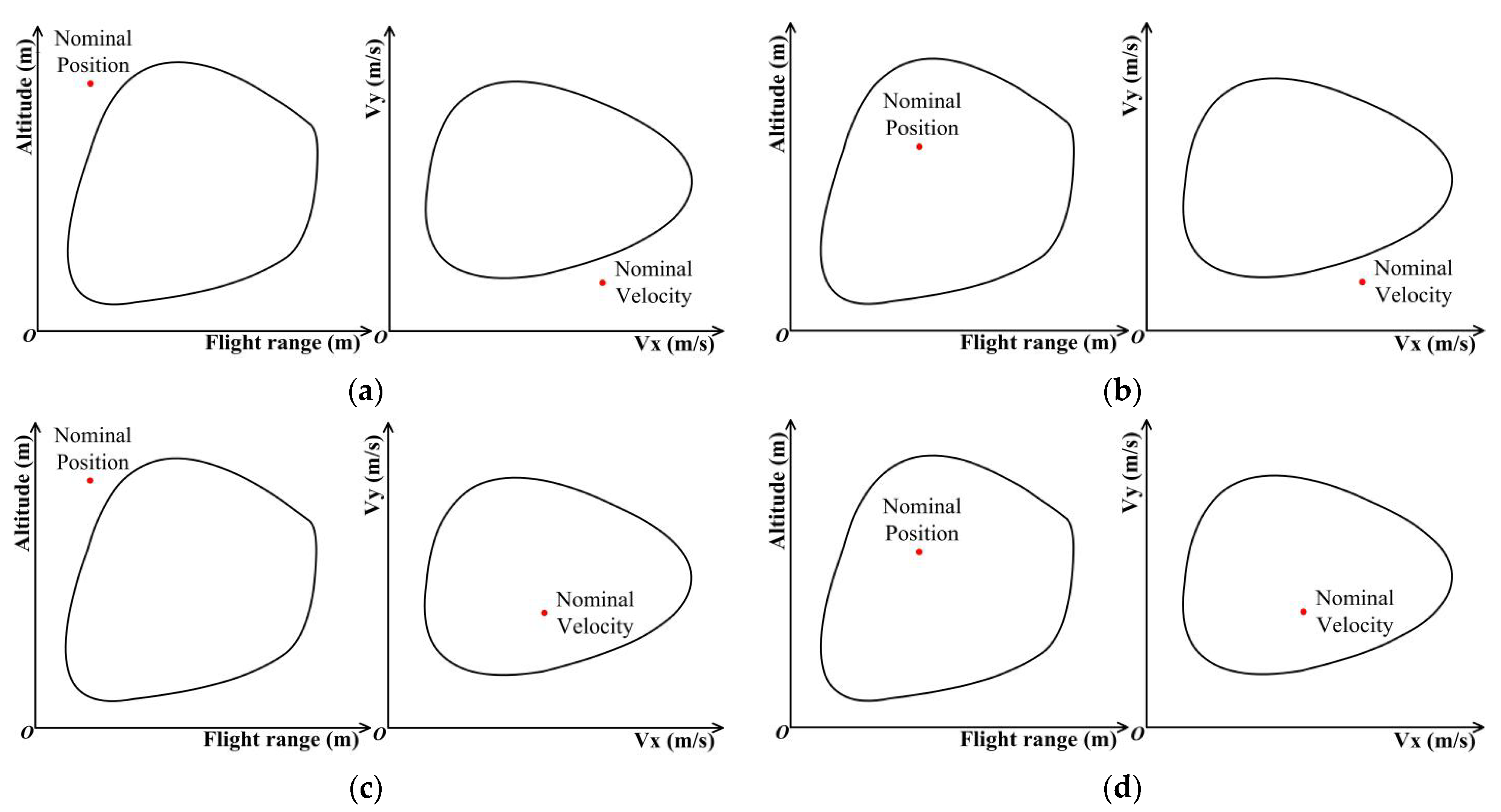
Considering the requirement of schematic presentation, the simplified CS is further decomposed into a two-dimensional position controllable subset and a two-dimensional velocity controllable subset along the nominal trajectory. The combination of these two controllable subsets reveals the comprehensive knowledge of the CS. The schematic diagrams of these two controllable subsets are illustrated in Figure 2.

In Figure 2a, the blue solid curve depicts the longitudinal position of the nominal trajectory, where R_x and R_y are its components along the x-axis and the y-axis of the LP coordinate system. Augmenting the longitudinal position curve with a third dimension of altitude, as plotted by the blue dash–dot line, the position controllable subset at different altitudes (corresponding to the specific velocities) can be conveniently visualized. For example, the red closed region in Figure 2a, which is parallel to the OR_xR_y plane, denotes the position controllable subset at the reference point. Likewise, the longitudinal velocity curve in Figure 2b, represented by its components along the x-axis and the y-axis of the LP coordinate system (denoted by V_x and V_y, respectively), is also augmented with the dimension of altitude to intuitively illustrate the velocity controllable subset.

An arbitrary element of CS represents a feasible initial condition for the powered landing phase, which is also the corresponding terminal of the preceding endo-atmosphere unpowered descent phase. Theoretically, the complete CS can be obtained by computing the position/velocity controllable subsets as the nominal endo-atmosphere unpowered descent trajectory is traversed, from its inception to touchdown. The traversal can be performed based on altitude due to its monotonic nature along the trajectory. This is also part of the reason for augmenting the nominal longitudinal position and velocity curves with an additional dimension of altitude.

4.2. Computation of the CS

The geometric feature of the CS for the powered landing problem has been roughly substantiated as convex [23,35,36], and the result of extensive numerical simulations further corroborates this understanding. Therefore, the aforementioned longitudinal position and velocity controllable subsets are approximated by a convex region.

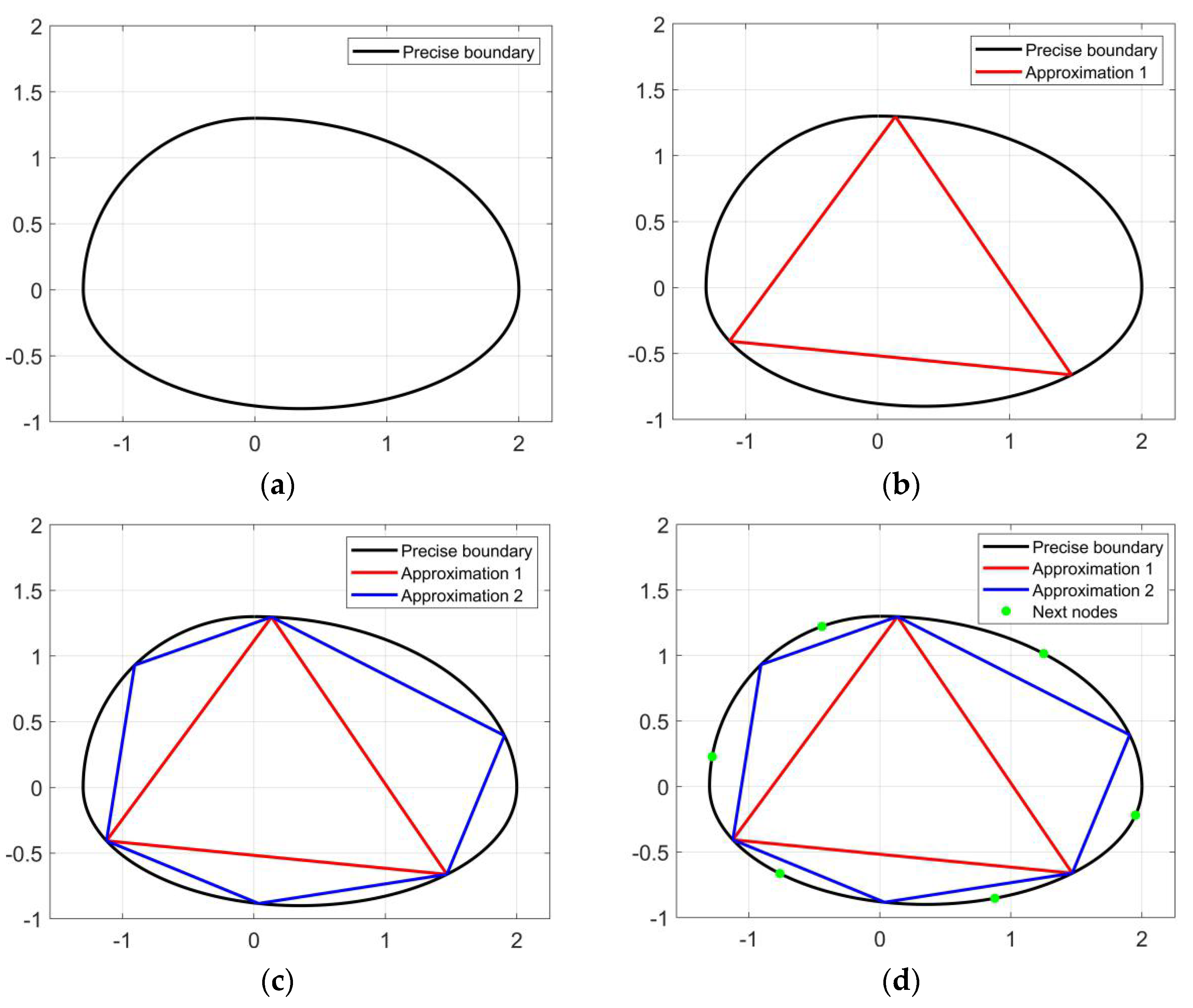
A convex region is determined by its boundary. For any given convex region, its boundary can be numerically obtained by successively implementing the polyhedron approximation method, as shown in Figure 3. To approximate the precise boundary, the polyhedron approximation method is initialized by generating an initial inner polyhedron. A simplest example is the triangle illustrated in Figure 3b. Note that the initial polyhedron is not constrained, allowing for its construction through multiple arbitrary feasible solutions.

Starting with a rough approximation of the initial polyhedron, a more accurate representation of the convex boundary can be obtained by successively extending the polyhedron. The extension is achieved by identifying points that are out of the current polyhedron but still within the convex region. The process can be expressed as follows:

$$\begin{array}{l}\mathrm{max:} \alpha \\ \mathrm{s}.\mathrm{t:} {\upsilon }_0=C\lambda , {\mathbf{1}}^T\lambda =1, \lambda \ge 0\\ \mathrm{ F}\left({\upsilon }_0+\alpha h\right)=0, G\left({\upsilon }_0+\alpha h\right)\le 0\end{array}$$

(33)

where C is the matrix containing the vertices of the open face, υ₀ represents a point on the open face, and h is the outward normal. Solving Equation (33) for each open face, points that are furthest from each open face can be obtained to extend the current polyhedron, as illustrated in Figure 3c,d. Repeating the process will eventually yield an approximation of the convex region with desirable accuracy. Since the outcomes are theoretically independent of the specific trajectory optimization method employed, we used the widely adopted successive convex optimization approach to compute the CS.

Although the construction of the initial polyhedron is not constrained, it significantly influences computational efficiency. Simulations reveal that an initial polyhedron with a larger “volume” typically requires fewer iterations to achieve a certain level of accuracy. Therefore, a method is in demand to construct a larger initial polyhedron.

Take the longitudinal position controllable subset for instance, solving for the highest/lowest possible altitudes, as well as the farthest/nearest possible flight range, can constitute an appropriate initial polyhedron, as shown in Figure 4.

The corresponding optimization problems of these three solutions, denoted by P-3, P-4, and P-5, are formulated as convex optimization problems similar to P-2, and the only differences are the objective functions.

• Formulation of P-3:
• Objective function:

$$\mathrm{min:} -r_y+{\sigma }_{\mathrm{ub}}\cdot ‖ub‖+{\sigma }_{\mathrm{aRb}}\cdot ‖aRb‖+{\sigma }_{\mathrm{dtb}}\cdot ‖dtb‖$$

(34)

• Formulation of P-4:
• Objective function:

$$\mathrm{min:} r_x+{\sigma }_{\mathrm{ub}}\cdot ‖ub‖+{\sigma }_{\mathrm{aRb}}\cdot ‖aRb‖+{\sigma }_{\mathrm{dtb}}\cdot ‖dtb‖$$

(35)

• Formulation of P-5:
• Objective function:

$$\mathrm{min:} r_y+{\sigma }_{\mathrm{ub}}\cdot ‖ub‖+{\sigma }_{\mathrm{aRb}}\cdot ‖aRb‖+{\sigma }_{\mathrm{dtb}}\cdot ‖dtb‖$$

(36)

It is worth noting that the solutions for P-3 and P-4 are special cases of the fuel-optimal powered landing problem, where all remaining propellant is consumed. Physically, it is evident that decelerating the reusable first stage from both the highest altitude and the farthest flight range requires the full use of the remaining propellant. In contrast, the solution for P-5 is not necessarily consistent with that of the fuel-optimal powered landing problem, since in this case, the altitude becomes the activated constraint rather than the propellant. Likewise, a large initial polyhedron for computing the controllable subset of the longitudinal velocity can be constructed in a similar way.

4.3. Application of the CS

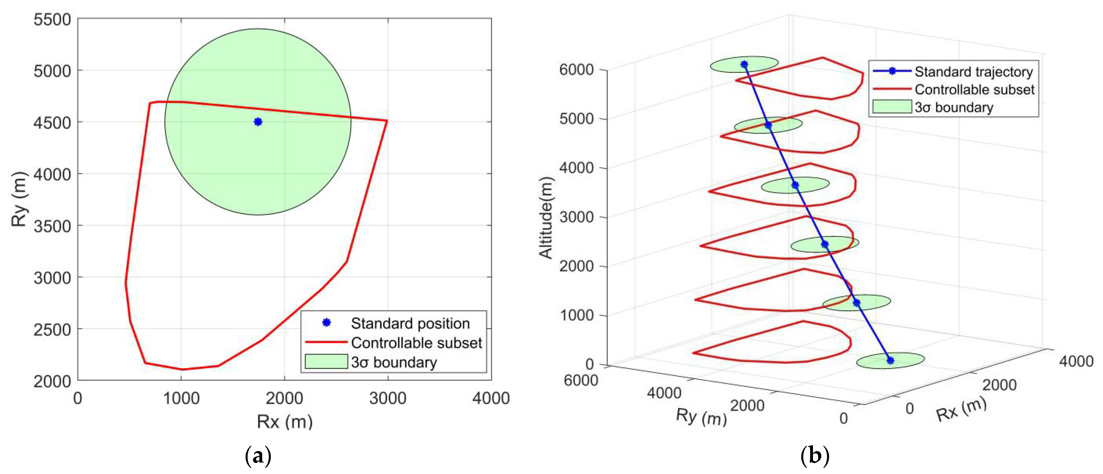
A straightforward application of the CS is to determine the physical feasibility of achieving a successful powered landing from specific flight states. Given the accurate controllable subsets of the longitudinal position and velocity, the feasibility of a powered landing can be assessed by verifying whether both the nominal position and velocity values fall within the respective controllable subsets, as illustrated in Figure 5.

Among all the possible cases shown in Figure 5, only Case-4 is feasible for achieving a successful powered landing under nominal conditions. The application of CS provides an effective and intuitive approach to distinguish between the viable and non-viable handover conditions for initiating the powered landing phase.

Since perturbations can make a considerable impact on the performance of powered landing in engineering practice, the state deviations from the nominal trajectory should be taken into account. Considering uncertainties, the CS can be further employed to calculate the probability of achieving a successful powered landing. Although many distributions can be adopted, the normal distribution is used in this paper following engineering conventions. Assuming that the uncertainties in position and velocity are mutually independent and both follow a normal distribution, the expressions for the actual position and velocity can be formulated as follows:

$$\left(r_x,r_y\right)\sim \mathrm{N}\left({\mu }_{\mathrm{r}x},{\mu }_{\mathrm{r}y},{\sigma }_{\mathrm{r}x}^2,{\sigma }_{\mathrm{r}y}^2,{\rho }_{\mathrm{r}}\right)$$

(37)

$$\left(v_x,v_y\right)\sim \mathrm{N}\left({\mu }_{\mathrm{v}x},{\mu }_{\mathrm{v}y},{\sigma }_{\mathrm{v}x}^2,{\sigma }_{\mathrm{v}y}^2,{\rho }_{\mathrm{v}}\right)$$

(38)

where μ_rx and μ_ry in Equation (37) are the values of the nominal longitudinal position along the x and y axes, respectively, while σ_rx and σ_ry are the corresponding standard deviations. ρ_r is the correlation coefficient, which measures the degree of linear correlation between the x and y components. By substituting the subscript “r” with “v”, the associated symbols for the longitudinal velocity in Equation (38) are defined.

Note that the normal distribution of the longitudinal position is two-dimensional, and the same applies to the longitudinal velocity. The explicit formulations of Equations (37) and (38) are as follows:

$$p(r_x,r_y)={\displaystyle \frac{1}{2\pi {\sigma }_{\mathrm{r}x}{\sigma }_{\mathrm{r}y}\sqrt{1-{\rho }_{\mathrm{r}}^2}}} \exp \left\{-{\displaystyle \frac{1}{2(1-{\rho }_{\mathrm{r}}^2)}}\left[{\displaystyle \frac{{(r_x-{\mu }_{\mathrm{r}x})}^2}{{\sigma }_{\mathrm{rx}}^2}}-2{\rho }_{\mathrm{r}}{\displaystyle \frac{(r_x-{\mu }_{\mathrm{r}x})(r_y-{\mu }_{\mathrm{r}y})}{{\sigma }_{\mathrm{r}x}{\sigma }_{\mathrm{r}y}}}+{\displaystyle \frac{{(r_y-{\mu }_{\mathrm{r}y})}^2}{{\sigma }_{\mathrm{r}y}^2}}\right]\right\}$$

(39)

$$p(v_x,v_y)={\displaystyle \frac{1}{2\pi {\sigma }_{\mathrm{v}x}{\sigma }_{\mathrm{v}y}\sqrt{1-{\rho }_{\mathrm{v}}^2}}} \exp \left\{-{\displaystyle \frac{1}{2(1-{\rho }_{\mathrm{v}}^2)}}\left[{\displaystyle \frac{{(v_x-{\mu }_{\mathrm{v}x})}^2}{{\sigma }_{\mathrm{vx}}^2}}-2{\rho }_{\mathrm{v}}{\displaystyle \frac{(v_x-{\mu }_{\mathrm{v}x})(v_y-{\mu }_{\mathrm{v}y})}{{\sigma }_{\mathrm{v}x}{\sigma }_{\mathrm{v}y}}}+{\displaystyle \frac{{(v_y-{\mu }_{\mathrm{v}y})}^2}{{\sigma }_{\mathrm{v}y}^2}}\right]\right\}$$

(40)

The values of the standard deviations in the above equations are selected based on the level of precision of the guidance, navigation, and control (GNC) system.

Since uncertainties are considered, it is still possible to achieve a successful powered landing even when the nominal position is beyond the corresponding position controllable subset, as illustrated in Figure 6a. The green region in Figure 6 defines the 3σ boundary of the position, which has a high probability of encompassing the actual value.

The physical feasibility of achieving a successful powered landing, solely in terms of longitudinal position, can be evaluated based on the probability of the actual position falling within the position controllable subset. This probability can be calculated as follows:

$$P_r={\displaystyle \underset{(r_x,r_y)\in C{S}_r}{\iint }p(r_x,r_y)dxdy}$$

(41)

where CS_r denotes the controllable subset of longitudinal position. As illustrated in Figure 6b, the portion of the 3σ boundary intersecting with the position controllable subsets varies along the trajectory. It implies the variation of the probability of feasibility and indicates the existence of a best handover condition to start the powered landing phase. A successful powered landing is likely when the nominal position falls within the corresponding controllable subset; however, the probability decreases when the nominal position falls outside.

The above analysis can also be applied to the longitudinal velocity, yielding similar regularities. Under the assumption that the uncertainties of the longitudinal position and velocity are independent, the overall probability of a successful powered landing, denoted by P, can be derived as follows:

$$P=P_r{P}_v={\displaystyle \underset{(r_x,r_y)\in C{S}_r}{\iint }p(r_x,r_y)dxdy}\times {\displaystyle \underset{(v_x,v_y)\in C{S}_v}{\iint }p(v_x,v_y)dxdy}$$

(42)

Herein, the correlation coefficients ρ_r in Equation (39) and ρ_v in Equation (40) are set to be zero for simplicity, indicating the mutual independence between the uncertainties in the x and y components of both position and velocity.

Once the controllable subsets along the standard trajectory are obtained, the corresponding probability of realizing a successful powered landing can be calculated based on the given standard deviations σ_rx and σ_ry. The probability quantifies the practical feasibility of the handover condition between endo-atmosphere unpowered descent and powered landing phases, which can serve as an indicator for appropriate decision-making.

5. Mission Re-Planning Strategy for Throttling Faults in Recovery

Acknowledging the significant impact of throttling capability on the physical feasibility of the powered landing, a mission re-planning strategy is proposed to address throttling faults during the recovery flight. Since the first possible detection of a throttling fault occurs in the re-entry powered descent phase, the mission re-planning strategy should primarily function in the subsequent endo-atmosphere unpowered descent and powered landing phases.

5.1. The Mission Re-Planning Scheme

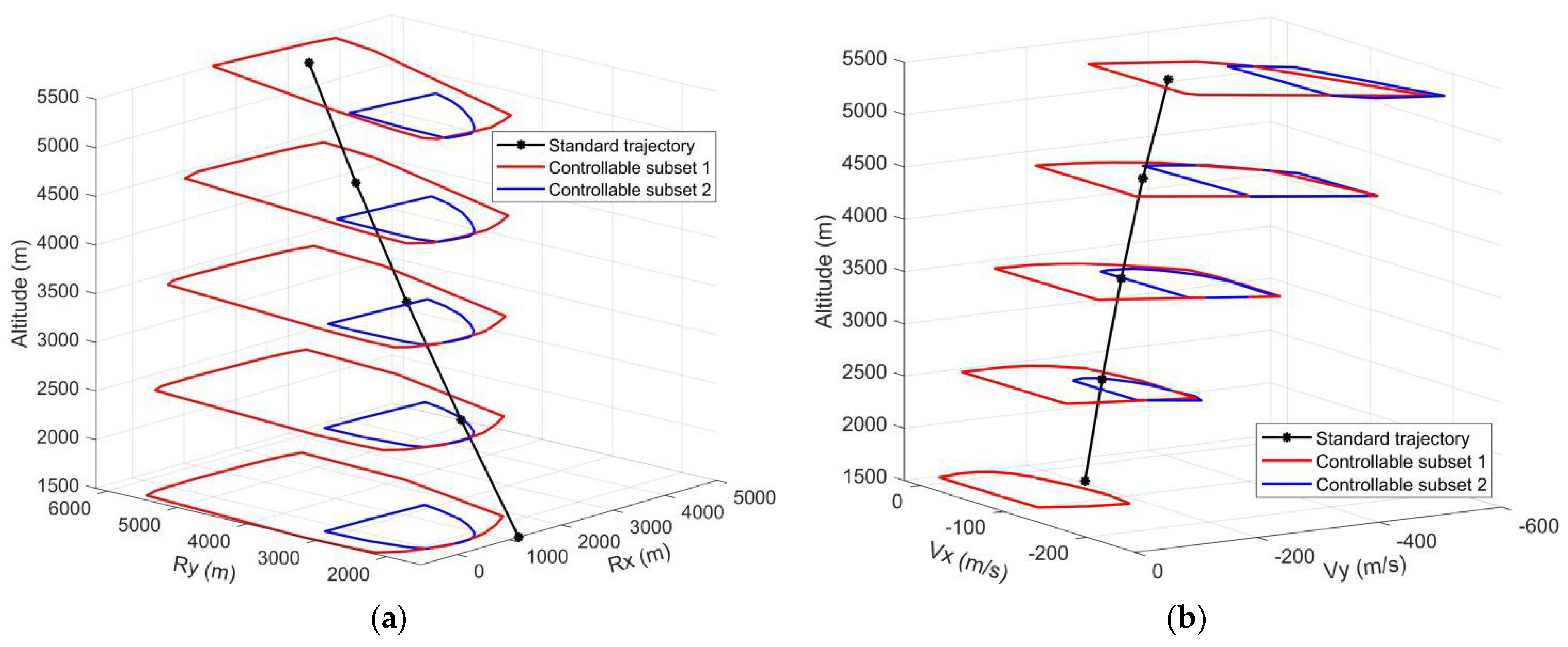
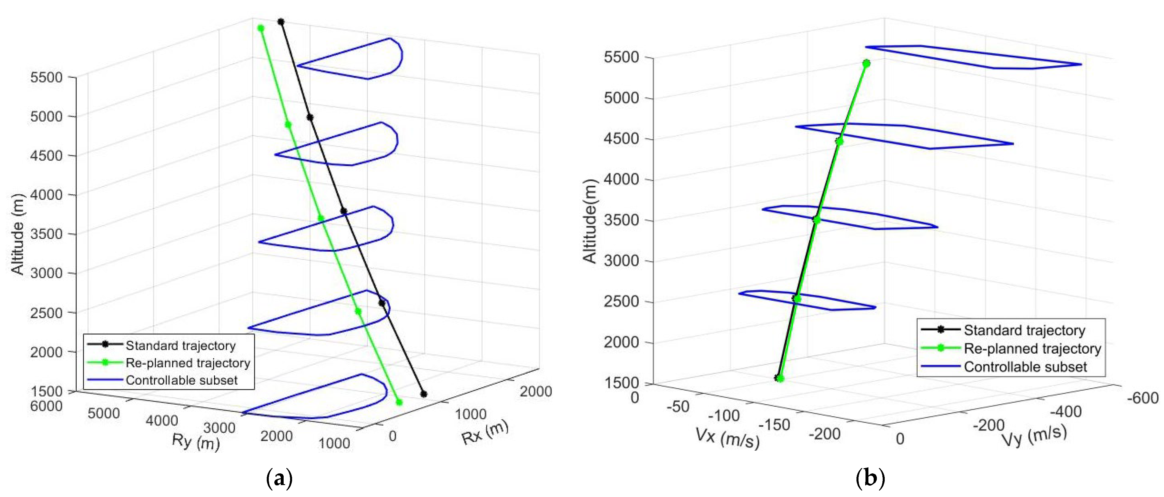
A throttling fault scenario is illustrated in Figure 7. In this case, controllable subset 1 shows the outcome of a nominal throttling capability, while controllable subset 2 reflects the performance of a reduced throttling capability. This figure clearly shows that both the position and velocity controllable subsets are greatly shrunk due to the reduction of the throttling capability. This reduction in the controllable subsets makes the location of the former feasible nominal condition very close to the boundaries, resulting in a higher risk of in-feasible powered landing.

Once a throttling fault is detected, re-planning the subsequent endo-atmospheric unpowered descent trajectory is a necessary and effective way to mitigate the adverse impacts. Starting from the terminal state of the re-entry powered descent phase, the endo-atmosphere unpowered descent trajectory can be re-planned by adjusting the designed angle of attack. Different designed angles of attack result in different standard trajectories, which further alter the intersection patterns between both the nominal position and velocity and their controllable subsets, as illustrated in Figure 8. An appropriately designed angle of attack can yield better intersection patterns, thus improving the probability of achieving a successful powered landing under throttling faults.

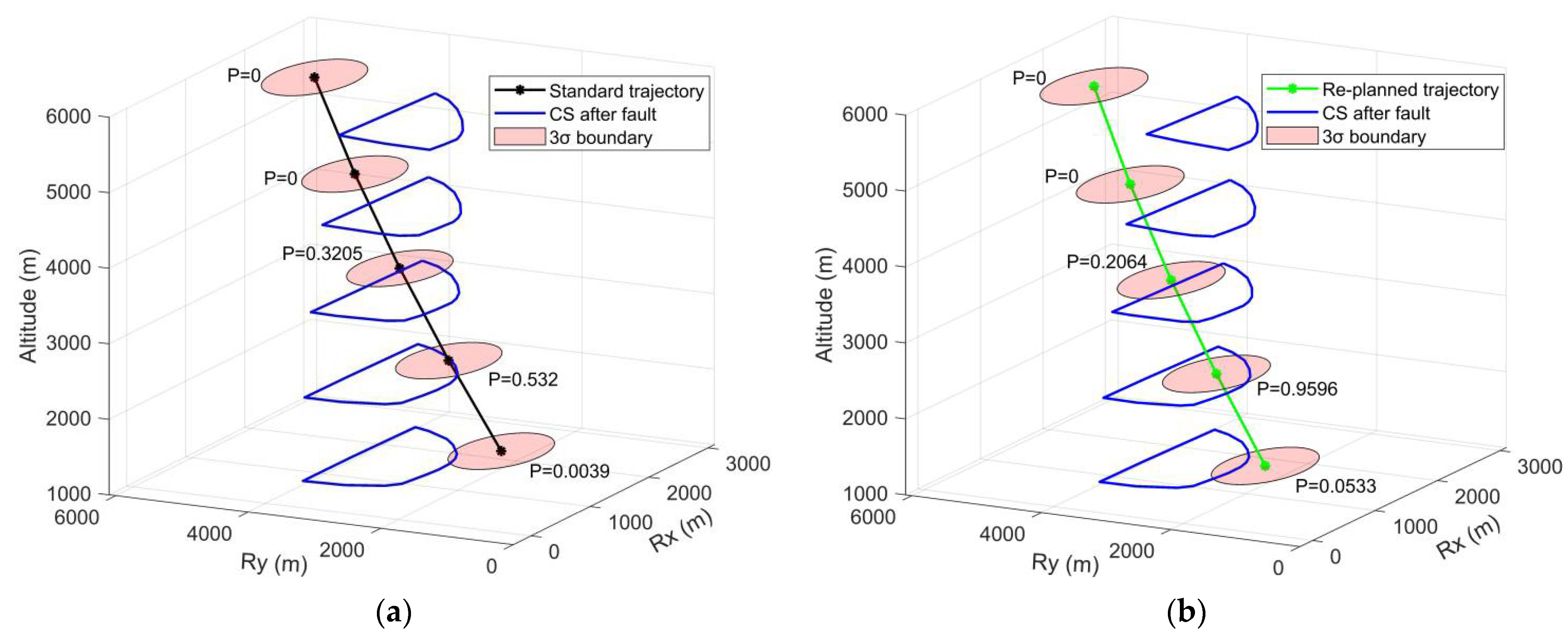
In addition to the designed angle of attack, the selection of the initial conditions under uncertainties for the powered landing phase can also significantly contribute to a successful powered landing. As discussed in Section 4.3, the probability-based assessment can facilitate the selection of the optimal handover condition. Taking the analysis of the longitudinal position as an example, Figure 9 compares the probabilities of physical feasibility between the standard trajectory and the re-planned trajectory.

Generally, the optimal handover condition should maximize probability along the trajectory. As shown in Figure 9a, the best initial position along the standard trajectory is at an altitude of 2.5 km, which provides a probability of only 53.2%. In contrast, the best initial position along the re-planned trajectory also occurs at an altitude of 2.5 km, but it significantly increases the probability to 95.96%.

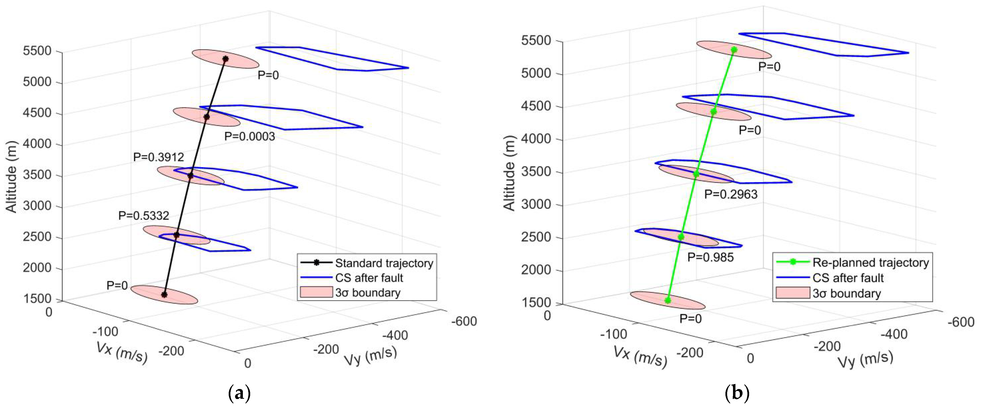
Applying the same analysis to the longitudinal velocity, the corresponding results are illustrated in Figure 10.

In this case, the optimal initial velocity is also observed at an altitude of 2.5 km. The probability of achieving a successful powered landing in terms of the initial velocity increases from 53.32% to 98.5% by re-planning.

To sum up, the comprehensive optimal handover condition can be determined by identifying the maximal joint probability of the initial position and velocity. In the presented case, the optimal handover condition is found at an altitude of 2.5 km, where the maximal joint probability is only 28.37% without re-planning, and it becomes 94.52% after appropriate re-planning.

5.2. The DNN-Based Prediction of the Re-Planning Parameters

Since mission re-planning is in urgent demand for online applications, enhancing computational efficiency is crucial from an engineering perspective. Leveraging the high efficiency of a well-trained deep neural network (DNN) in nonlinear mapping, a DNN-assisted mission re-planning scheme is proposed to meet real-time requirements.

Given the post-fault throttling capability, a DNN is designed to assess the physical feasibility of a specific nominal condition and predict the probability of achieving a successful powered landing under that condition. Consequently, the feasibility indicator and the probability constitute the two-dimensional output of the DNN.

The input of the DNN includes fault information, specific handover conditions, and stochastic distributions of flight states. In this paper, fault information is exactly the maximal throttling capability. As outlined in Section 4, the handover condition is uniquely defined by the designed angle of attack during the endo-atmosphere unpowered descent phase and the monotonically varying altitude. Section 4 also details the use of Gaussian distribution to model the stochastic distributions of flight states, as expressed in Equation (39) and Equation (40). These distributions are determined by the standard deviations of position and velocity, with the nominal condition serving as the mean. Further assuming that the standard deviations are identical across orthogonal directions, these distributions can then be determined by just two specific standard deviation values. Therefore, the input of the DNN consists of five elements: the post-fault throttling capability, the designed angle of attack, the engine re-ignition altitude, and two standard deviations.

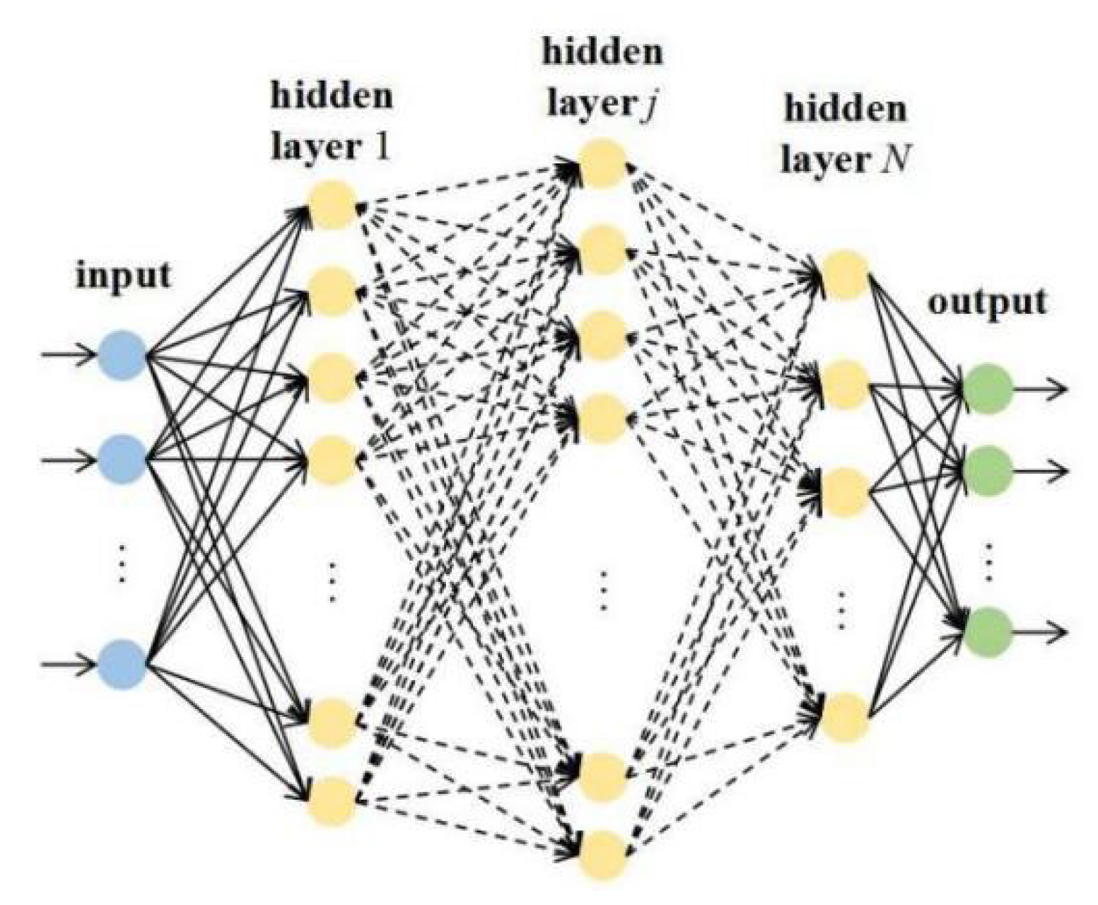
On this basis, a fully connected DNN structure can be applied to learn the underlying relationship between the input and output elements, as illustrated in Figure 11. It consists of three hidden layers with 16, 8, and 8 neurons, respectively. The activation function used in the first hidden layer is the sigmoid function, and the hyperbolic tangent function is employed in the latter two hidden layers.

The samples used in this paper are generated by numerical simulation. The set of inputs is constructed by sampling each input element within its possible range. For a given input, the output is determined by a three-step process. Firstly, the nominal trajectory, starting from the end of the re-entry powered descent phase to touchdown, is integrated using the angle of attack. Secondly, the specific handover condition corresponding to the input engine re-ignition altitude is identified. Under this condition, the controllable subsets are computed, with the post-fault throttling capability taken into account. Finally, the physical feasibility of the nominal condition is assessed by examining its inclusion within the controllable set. The probability of achieving a successful powered landing under uncertainties is then calculated by integrating the given uncertain distributions over the controllable set.

To reduce the sample size, the set of inputs is divided into two parts in practice, each of which is treated differently in the sampling process. The first part includes the post-fault throttling capability, the designed angle of attack, and the engine re-ignition altitude. When re-planning, these elements are typically considered to be continuous within their respective possible ranges. Therefore, the Latin hypercube sampling (LHS) is suitable for sampling these input elements to achieve better coverage of the input space. The second part comprises the standard deviations for both position and velocity, which are only used to calculate the probability. Their precise values are neither practical to obtain nor necessary for application in practice, thus several preset discrete values are adequate. This allows a reduction in the number of required training samples.

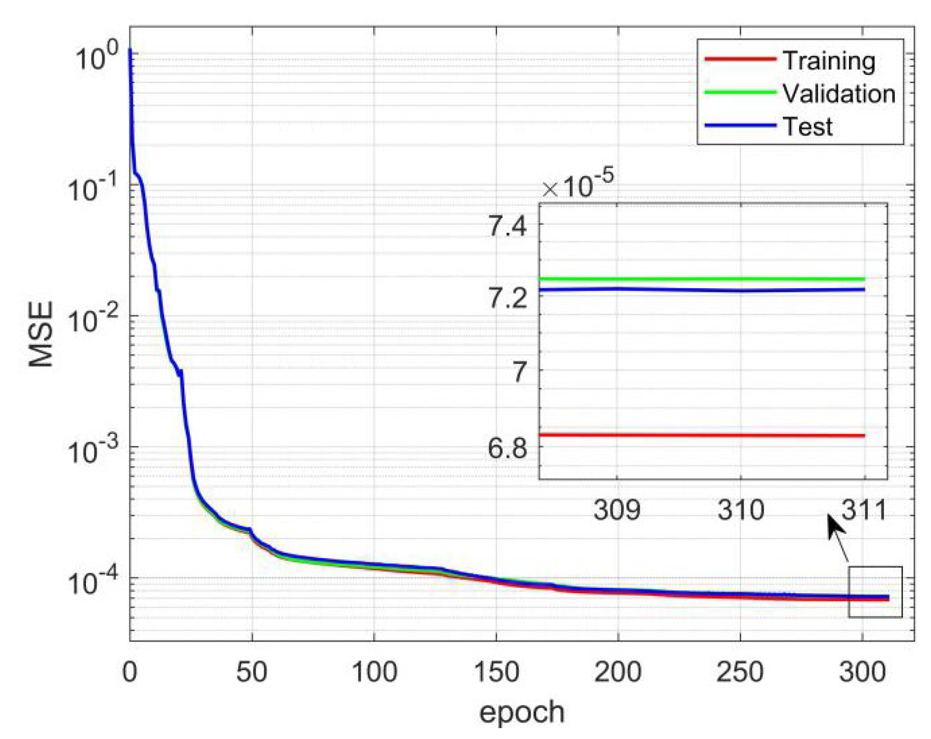
The samples are divided into a training set, a test set, and a validation set in the ratio of 70%, 15%, and 15% to train the DNN. The loss function is defined by the mean squared error (MSE), which is subsequently minimized using the Levenberg–Marquardt algorithm. The training process is shown in Figure 12.

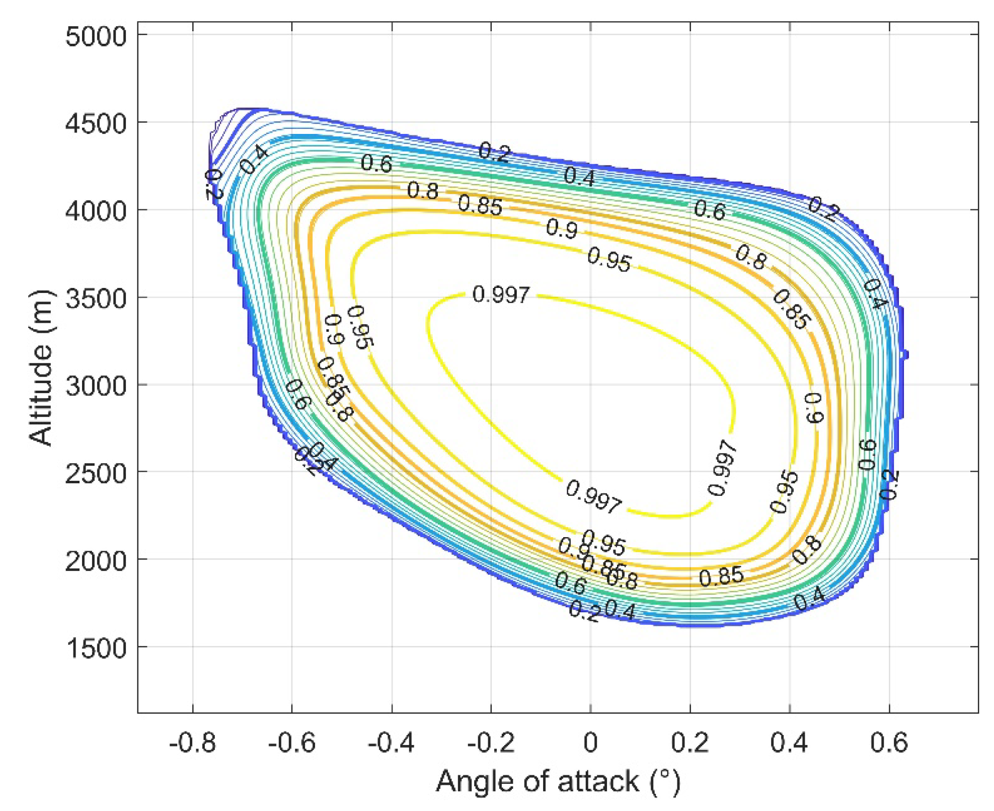
Given the post-fault throttling capability and the standard deviations of flight states, a forward propagation of the trained DNN can predict the feasibility index and probability for a specific handover condition. Therefore, the appropriate mission re-planning parameters can be obtained by evaluating all possible handover conditions and selecting the one with the highest probability. The comprehensive evaluation can be implemented straightforwardly by traversing the possible range of engine re-ignition altitude and the designed angle of attack, as illustrated in Figure 13.

Based on the probability predictions for all possible combinations, the optimal re-planning parameters (specifically, the designed angle of attack and the engine re-ignition altitude) can be selected accordingly. Typically, the center of the region enclosed by the highest probability contour is regarded as the best re-planning solution, as it is believed to maximize the probability of achieving a successful powered landing after a fault.

6. Simulations

In this section, the accuracy of the CS computed using the polyhedron approximation method is verified first. Then, several throttling fault scenarios are designed to validate the effectiveness of the proposed re-planning strategy during the recovery flight. Besides, the computational efficiency of the re-planning scheme is also evaluated due to the requirements for online application.

The following simulation scenarios are designed based on the same reusable launch vehicle, the critical parameters of which are listed in

Table 1. The critical parameters of the reusable launch vehicle.

Parameters	Values	Units
Initial mass after the re-entry powered descent phase	67,400	kg
Dry mass	57,000	kg
Specific impulse	335	s
Nominal throttling capability	0.55–1.0	/
Maximum thrust magnitude	1,250,000	kN
Maximum thrust magnitude adjustment rate	200,000	kN/s
Aerodynamic reference area	19.6	m2

. Simulations begin from the terminal of the re-entry powered descent phase, and they are implemented in MATLAB 2017a software on a desktop equipped with an Intel Core i7-10700 processor running at 2.90 GHz.

6.1. Accuracy of the CS Computation

Monte Carlo simulation (MCS) is utilized to validate the accuracy of the controllable subsets computed by the polyhedron approximation method. For a given combination of longitudinal position and velocity, the corresponding controllable subsets are determined using the polyhedron approximation method. Subsequently, multiple fuel-optimal powered landing problems are generated by randomly selecting initial positions/velocities within a certain domain. The solutions to these problems are then evaluated to confirm their feasibility.

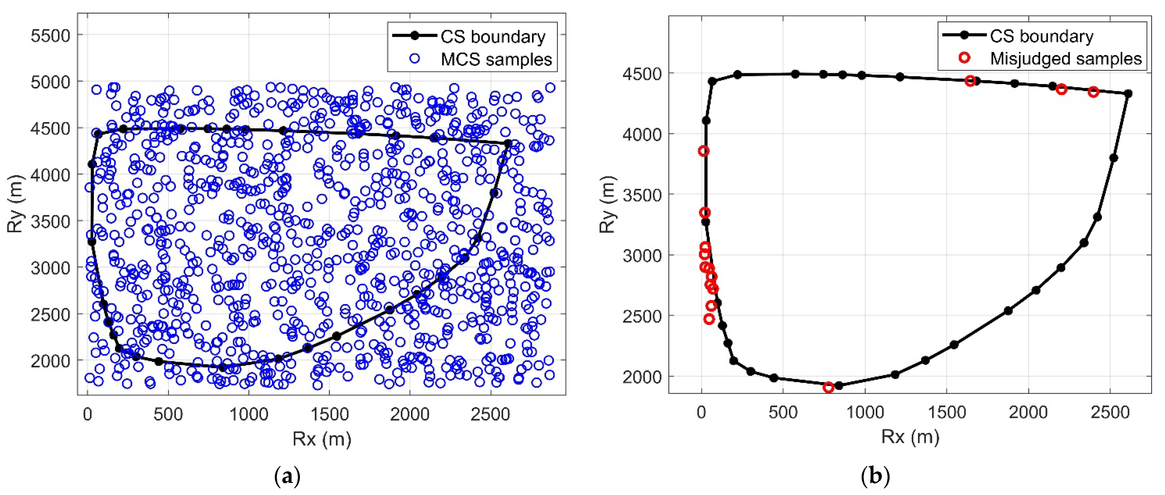
By setting the designed angle of attack to zero, a nominal trajectory is obtained for the subsequent example. As illustrated in Figure 14, the position controllable subset corresponding to the nominal velocity at an altitude of 3 km is computed, and an MCS with 1000 samples is then conducted to assess the accuracy.

Figure 14b statistically shows that only 15 out of the 1000 randomly selected MCS samples are misjudged. Thus, the accuracy of the position controllable subset in this example reaches 98.5%. Additionally, all misjudged samples are located extremely close to the boundary, indicating a high level of reliability in computing the CS using polyhedron approximation.

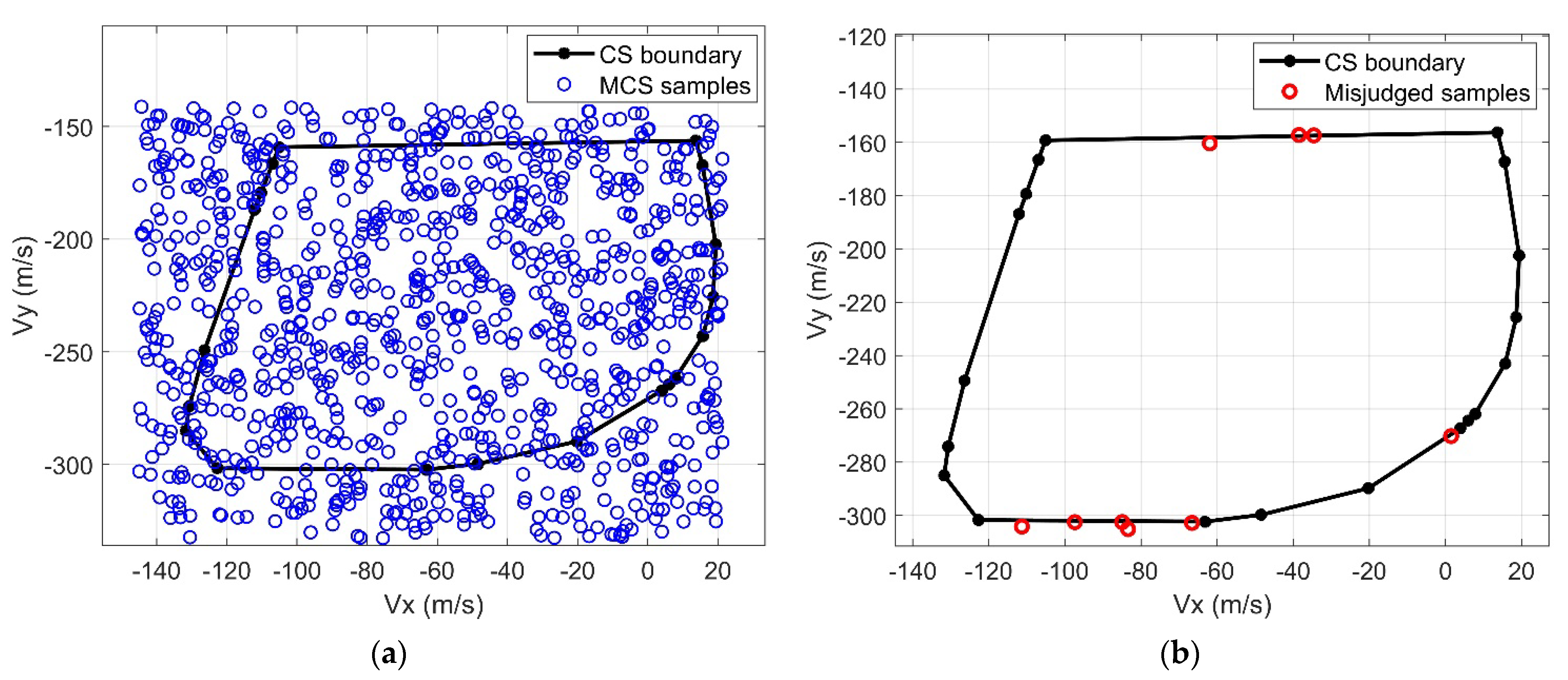
Similarly, a 1000-sample MCS is also employed to assess the accuracy of the velocity controllable subset associated with the nominal position at the same altitude of 3 km. The results are presented in the following Figure 15.

In this example, the accuracy of the velocity controllable subset is 99.1%, with only nine misjudged samples located close to the boundary as well.

6.2. Re-Planning Under Throttling Faults

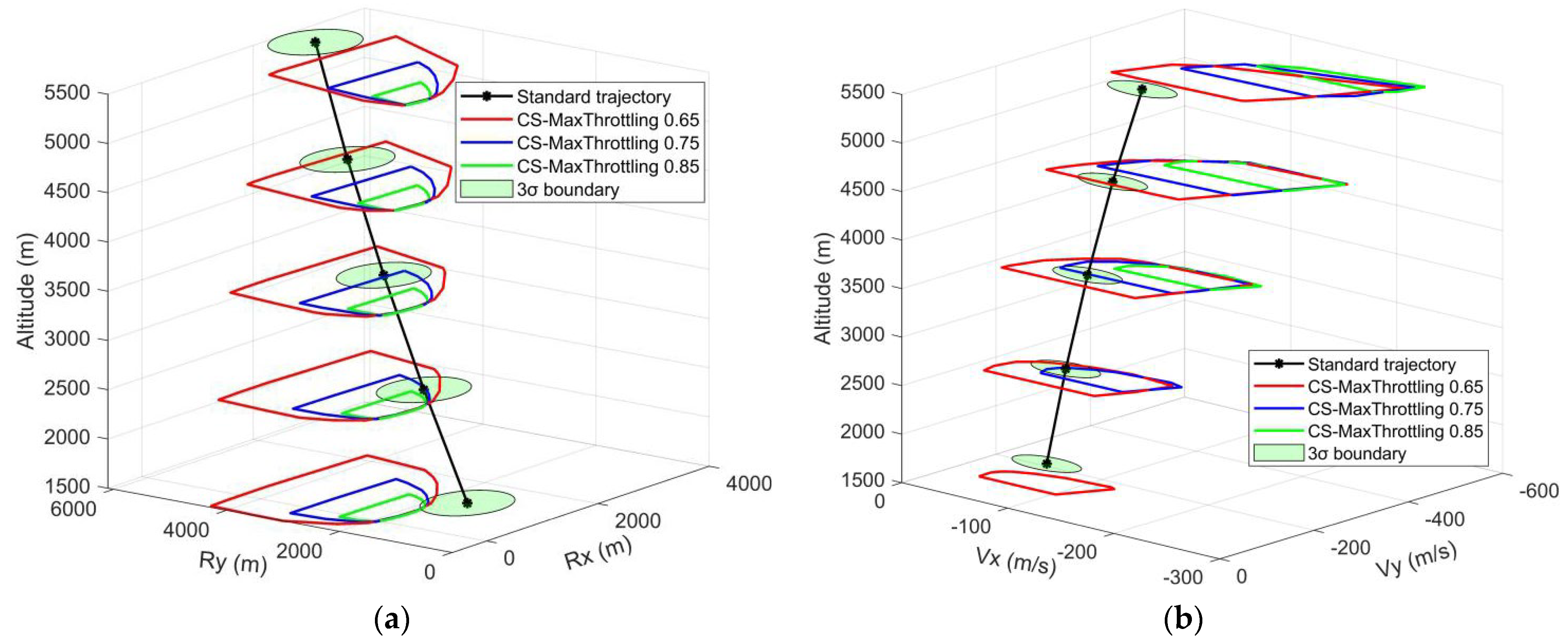
Given the throttling faults with maximal throttling capabilities of 65%, 75%, and 85% of the nominal thrust magnitude, Figure 16 illustrates the controllable subsets corresponding to different handover conditions along the standard trajectory at discrete altitudes. The standard deviations in the following examples are set to be 100 m for the position and 15 m/s for the velocity.

As introduced in Section 5, the first step of re-planning is changing the designed angle of attack to adjust the nominal trajectory during the endo-atmosphere unpowered descent phase. Then, the probability of achieving a successful powered landing can be evaluated based on the computation of CS along the adjusted nominal trajectory. The application of a DNN enables a thorough investigation of the entire re-planning design space. Consequently, the re-planning solution, which consists of the designed angle of attack and the altitude associated with the optimal handover condition, can be directly obtained.

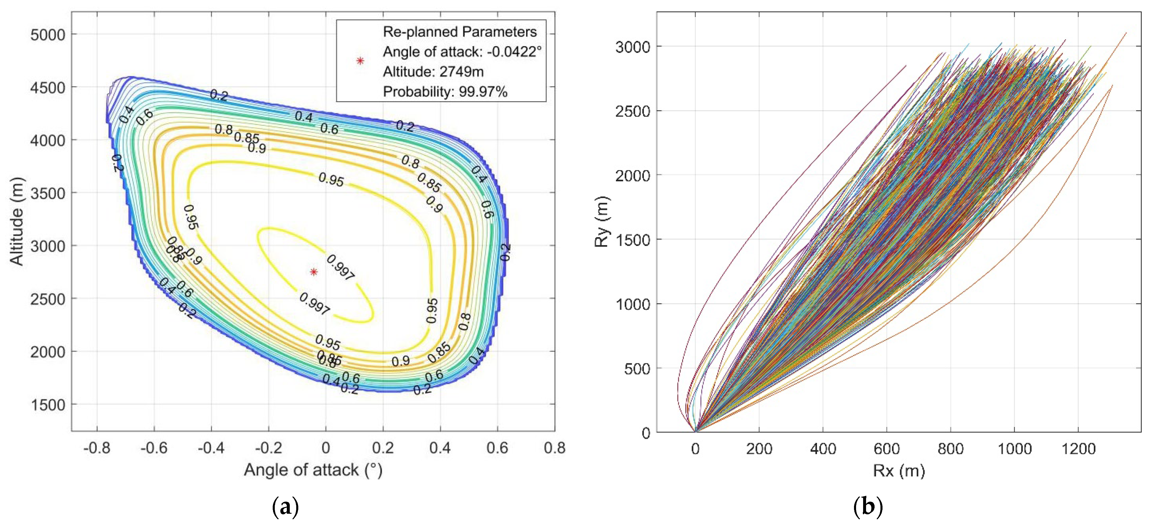
For the throttling fault with a maximal throttling capability of 65% of the nominal thrust magnitude, the probability-based analysis and the performance of the final re-planning solution are shown in Figure 17.

As indicated by the CS analysis, the final re-planning parameters are composed of the designed angle of attack of −0.0422° and the engine reignition altitude of 2749 m. The DNN predicts a 99.97% probability of feasibility for this re-planning solution. To verify the solution, a 1000-sample MCS is conducted. As all samples achieve a pinpoint landing, the effectiveness of the re-planning is confirmed.

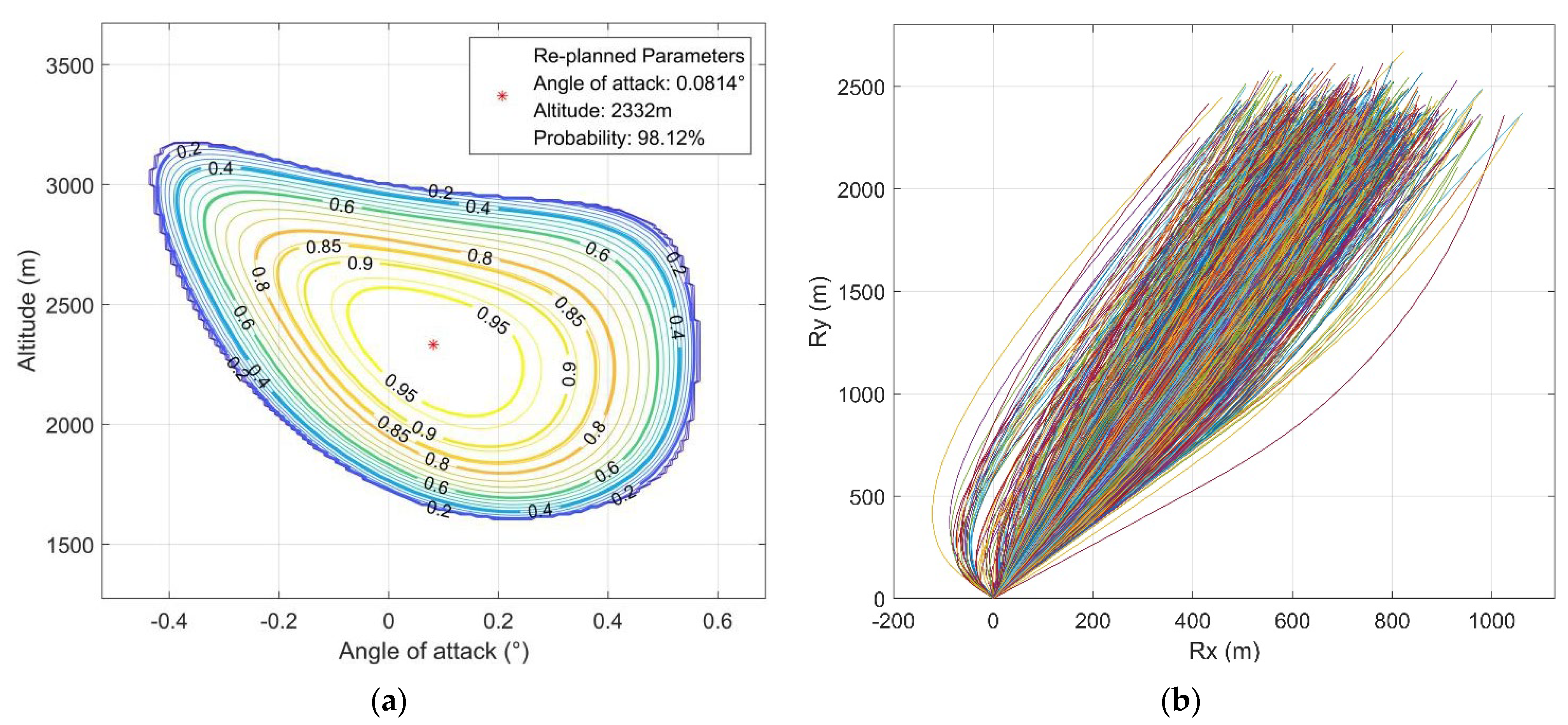
For the throttling fault with a maximal throttling capability of 75% of the nominal thrust magnitude, the probability-based analysis and the performance of the final re-planning solution are shown in Figure 18. Compared with Figure 17a, the region and probability are reduced, reflecting the adverse impact of the throttling fault.

In this case, the suggested re-planning solution provides a 98.12% probability of achieving pinpoint landing, with the re-planned angle of attack of 0.0814° and engine reignition altitude of 2332 m. Only 23 out of 1000 samples do not achieve successful powered landing in the 1000-sample MCS, indicating a 97.7% probability of feasibility.

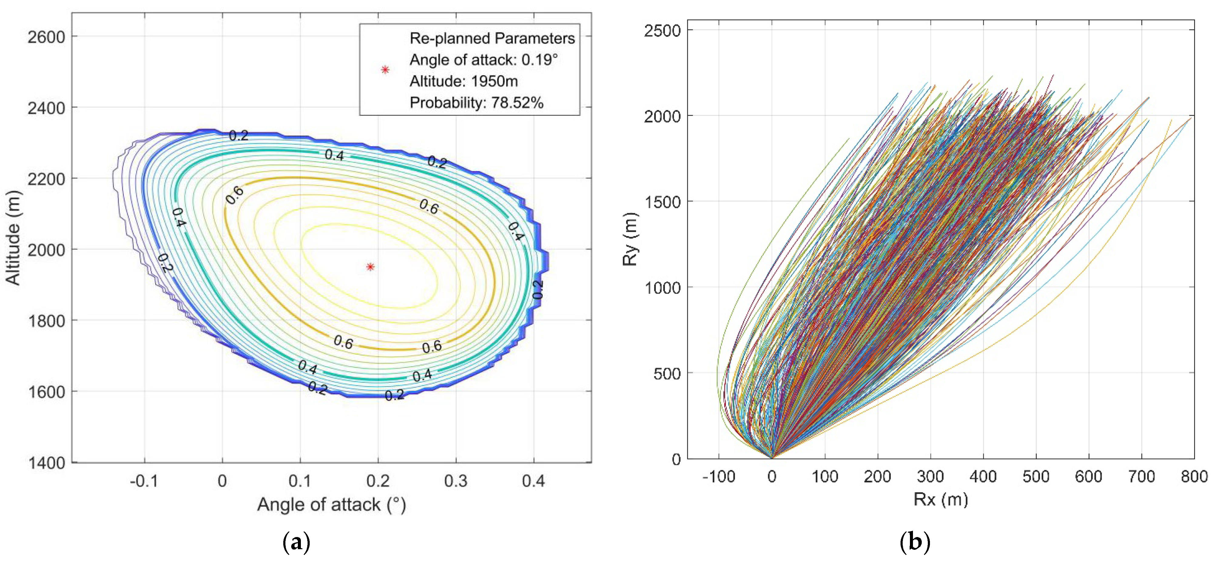
For the throttling fault with a maximal throttling capability of 85% of the nominal thrust magnitude, the probability-based analysis and the performance of the final re-planning solution are shown in Figure 19.

In this case, re-planning can only maximize the probability of feasibility to the level of 78.52% due to the significantly reduced throttling capability. The 1000-sample MCS indicates a 67.3% probability of feasibility, which is a little bit less than the predicted probability. This difference is brought by the varying engine reignition altitudes in the MCS, while the predicted value is at the optimal condition.

The average computing time of each case is on the level of 280 milliseconds on the MATLAB 2017a software platform with a desktop equipped with an Intel Core i7-10700 processor at 2.90 GHz. However, a minimum of 250 trajectory optimization problems should be solved to obtain an investigation of the re-planning design space without DNN. Each individual optimization requires 3 s on average, thus the estimated computing time without DNN is about 750 s. Therefore, the application of DNN is very promising in realizing online applications.

7. Conclusions

This paper proposes a mission re-planning scheme for the recovery flight of reusable launch vehicles to address throttling faults. To obtain an appropriate re-planning solution, the following methods are developed:

(1)

The controllable set concept is introduced to quantify the influence of throttling capability on the physical feasibility of achieving a successful powered landing. It is computed by using the polyhedron approximation method and convex optimization. Based on the controllable set, the probability of realizing a soft landing can be evaluated with deviations from the nominal conditions taken into account.

(2)

A re-planning scheme is proposed to deal with throttling faults in recovery flight, based on the controllable analysis. In this scheme, the designed angle of attack during the endo-atmospheric descent phase needs to be adjusted to improve the potential handover conditions, and the probability-based optimal handover condition is then determined for the highest probability of achieving a successful recovery flight.

(3)

A DNN is constructed to enhance the computational efficiency of the controllable analysis. This enables a comprehensive investigation of the re-planning design space, providing a valuable foundation for obtaining appropriate re-planning parameters in real time.

Numerical simulation results show that the broader the range of throttling capability is, the higher the physical feasibility of a pinpoint landing can be. Following the proposed re-planning scheme, the probability of a successful powered landing can be maximized by properly selecting the designed angle of attack and the engine reignition conditions. Meanwhile, the scheme can be conducted in real time with the application of a DNN.