Deep Reinforcement Learning-Based Guidance Law for Intercepting Low–Slow–Small UAVs

Abstract

Low, small, and slow (LSS) unmanned aerial vehicles (UAVs) pose great challenges for conventional guidance methods. However, existing deep reinforcement learning (DRL)-based interception guidance law has mostly focused on simplified two-dimensional planes and requires strict initial launch scenarios (constructing collision triangles). Designing more robust guidance laws has therefore become a key research focus. In this paper, we propose a novel recurrent proximal policy optimization (RPPO)-based guidance law framework. Specifically, we first design initial launch conditions in three-dimensional space that are more applicable and realistic, without requiring to form a collision triangle at the initial launch. Then, considering the temporal continuity of the seeker’s observations, we introduce the long short-term memory (LSTM) networks into the proximal policy optimization (PPO) algorithm to extract hidden temporal information from the observation sequences, thus supporting the policy training. Finally, we propose a reward function based on velocity prediction and overload constraints. Simulation experiments show that the proposed RPPO framework achieves an interception rate of 95.3% and a miss distance of 1.2935 m under broader launch conditions. Moreover, the framework demonstrates strong generalization ability, effectively coping with unknown maneuvers of UAVs.

1. Introduction

With the continuous development of modern technology, precision guidance technology has become an indispensable core technology, widely applied in various tasks such as unmanned aerial vehicles (UAVs) and defense systems. However, traditional precision guidance methods face significant challenges when dealing with certain types of low, slow, and small (LSS) UAVs. As a new type of force, LSS UAVs have characteristics of low flight altitude, slow speed, and small radar cross-section (RCS). Existing defense systems are high-cost and cannot play a role in the engagement scenarios of LSS UAVs. Therefore, it is necessary to study a defender with low cost and low overload to effectively intercept LSS UAVs.

Successful interception requires a minimal miss distance and a relatively uniform distribution of the ballistic overload. Based on the defender’s kill radius, the required miss distance is 5 m. Due to the limited maneuverability, the entire trajectory’s overload needs to be planned, which further complicates the interception problem. Proportional navigation guidance (PNG) [1], due to its simple computation and strong applicability, has become one of the most widely used guidance schemes. PNG primarily focuses on concentrating the overload during the terminal phase. For interceptors with limited available overload, the interception accuracy significantly decreases when the target is in a maneuvering state. Compared with PNG, augmented proportional navigation guidance (APNG) [2] introduces compensation for maneuvering targets, which can reduce the end effector overload to a certain extent. For a defender with a low overload capacity, the overload calculated by these traditional methods is too concentrated and unevenly distributed, which may result in limited interception effectiveness.

The development of modern control theory has provided new avenues for addressing the design problems of guidance law in intercepting maneuvering UAVs. Optimal guidance law [3], sliding mode control-based guidance law [4,5], and similar approaches have attracted significant attention from numerous researchers. Asher et al. [6] were the first to introduce optimal control theory into the interception problem of maneuvering targets and provided an analytical derivation of the optimal closed-loop guidance law for a missile with limited bandwidth in engaging maneuvering targets. Dun et al. [7] applied optimal control theory and incorporated energy management considerations, thus deriving an optimal guidance law that addresses high-speed and maneuvering targets. Kim et al. [8] employed optimal control concepts to provide a unified formulation for the optimal collision course law for targets with arbitrary acceleration or deceleration, ensuring the optimality of the guidance commands even in non-linear engagement scenarios. In [9], Shima et al. adopted sliding mode control as the primary approach for the design of guidance laws in interception scenarios. They developed a guidance law capable of dealing with all engagement geometries. However, the guidance law could not guarantee error convergence in a finite time. Zhang et al. [5] proposed an optimal sliding mode guidance law, in which an adaptive sliding mode switching term was designed to address prediction error and actuator saturation, effectively reducing both the interceptor’s energy consumption and the terminal acceleration commands. Zheng et al. [10] presented an adaptive sliding mode guidance law that overcomes the conventional issues of large initial control input and chattering in traditional sliding mode guidance. Guidance laws based on modern control theory often require more observational information. In practical situations, due to the limited observability of sensors, many states are difficult to obtain, and partial observability challenges remain unresolved in modern control methods.

With the development of artificial intelligence technologies, reinforcement learning (RL) [11] and deep reinforcement learning (DRL) [12] algorithms have become the core data-driven paradigms for solving complex decision optimization and control problems. These algorithms have already been widely applied in fields such as gaming [13], robotics [14,15], and autonomous driving [16]. RL is based on the Markov decision process (MDP), where an agent interacts with the environment to continuously learn the optimal policy. The core concept is to approximate the policy and value function using neural networks, improving learning efficiency and stability through techniques such as experience replay [17] and target networks. DRL combines the advantages of deep learning and reinforcement learning [18], enabling it to handle high-dimensional state spaces and continuous action spaces [19]. To overcome the limitations of traditional guidance methods, the RL and DRL algorithms have also been used to design guidance laws. Hu et al. [20] proposed a second-order sliding mode guidance law with terminal impact angle constraint by integrating the twin-delayed deep deterministic policy gradient (TD3) [21] framework with nonsingular terminal sliding mode control (NTSM), effectively mitigating the inherent chattering issue associated with sliding mode control. Gaudet et al. [22] applied reinforcement meta-learning (Meta-RL) to address the problem of intercepting maneuvering targets in outer space. This method generates guidance commands using only the LOS angle and the LOS angular rate as observation values. Compared to traditional RL, an agent trained with Meta-RL enhances its generalization ability to uncertain scenarios. The authors also extended this method to applications such as lunar landing [23] and asteroid exploration, proving the feasibility of RL in practical applications [24,25]. Qiu et al. [26] proposed a recorded recurrent-twin delayed deep deterministic (RRTD3) policy gradient algorithm for intercepting maneuvering targets in the atmosphere. This approach addresses the impact of uncertainty and observation noise by modeling the engagement scenario as a partially observable Markov decision process (POMDP). Additionally, the recurrent neural network layer was incorporated into the policy network, improving training speed and stability [27].

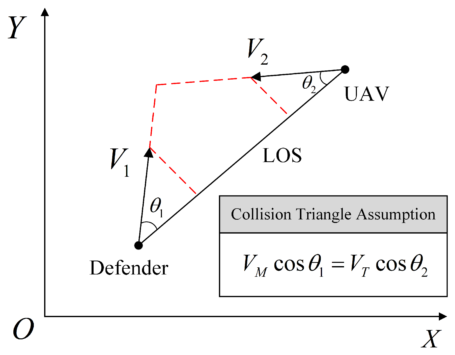
Despite the significant progress of DRL algorithms in guidance law design, current research universally relies on simplifying assumptions. Existing works typically reduce complex engagement scenarios to a two-dimensional plane and provide the defender with an ideal initial launch angle by pre-setting a collision triangle [28], as shown in Figure 1. While this idealized setup accelerates algorithm convergence by shrinking the state space and circumventing the challenge of correcting large initial heading errors, it does so at the cost of model fidelity. However, to ensure rapid response, radar is typically not employed to provide initial launch angles for low-overload defenders, rendering this assumption invalid in our study. Therefore, our work directly addresses the core challenge that arises when these idealized constraints are removed, namely, the expanded exploration space in a three-dimensional environment without prior guidance information, which results in inefficient training and even failure to converge with existing DRL methods.

In this work, we propose a novel recurrent proximal policy optimization (RPPO) guidance law framework, designed to solve the challenge of high-precision interception of LSS UAVs by a low-overload defender with limited observations. The main contributions of our work are as follows:

• The RPPO guidance law framework for intercepting LSS UAVs is proposed, which leverages a recurrent neural network to extract temporal information from the observation sequence and address the limitations of traditional DRL algorithms in partially observable scenarios.
• A three-dimensional guidance law modeling method is proposed, which frames the interception problem as a POMDP model and introduces a random launch angle mechanism that does not rely on the collision triangle, thereby broadening the launch conditions.
• A novel reward function is proposed, which leverages UAV velocity prediction to accelerate convergence and incorporates overload distribution constraints to improve interception accuracy. This approach addresses the sparse reward problem and improves training performance.

The remainder of this paper is organized as follows: In Section 2, the engagement scenario is constructed, followed by a brief discussion of the reinforcement learning framework and PPO algorithm. Section 3 mainly introduces the proposed RPPO algorithm framework and the implementation details in the combat scenario. The simulation experiments are conducted in Section 4 to verify the performance of the proposed method. The conclusion are presented in Section 5.

2. Problem Formulation

This section primarily introduces the relative motion equations between the missile and the UAV in three-dimensional space, as well as some specific details within the training environment. Before proceeding, we first present the following widely accepted assumptions [29,30]:

Assumption 1: The entire engagement process is modeled as a head-on engagement scenario, where the defender is fired towards the UAV to ensure that the defender and the UAV move closer to each other. This assumption is based on the fact that, in interception problems, the defender intercepts the UAV in a head-on engagement [31].

Assumption 2: The influence of gravity is neglected throughout the guidance process. The rationale behind this assumption is that, during the initial development of new guidance laws, ignoring gravity is a common practice [32].

Assumption 3: The velocities of both the defender and the UAV are assumed as constants. This assumption is founded on the observation that the terminal guidance duration is relatively short.

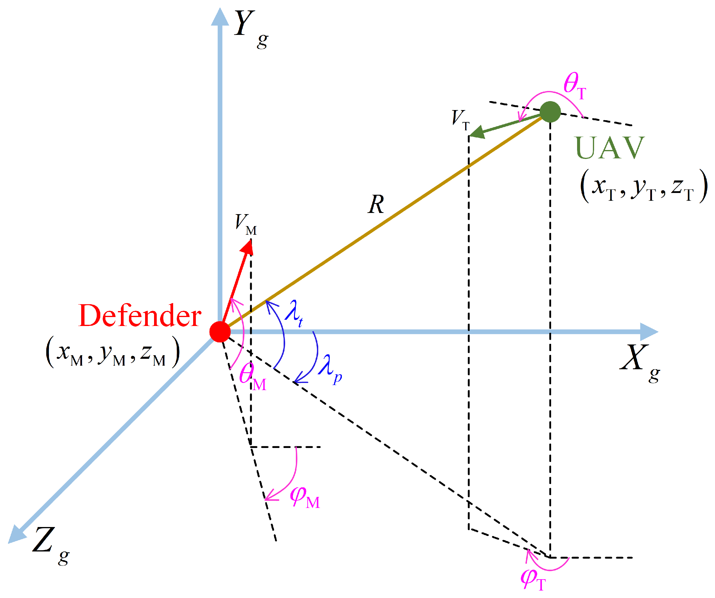
In this study, the three-dimensional engagement scenario is depicted as shown in Figure 2. M represents the defender fired from the origin of the coordinate system, while T represents the incoming UAV from a distant location. The mission of M is to intercept T.

2.1. Equations of Engagement

A three-dimensional spatial coordinate system $O-X_g{Y}_g{Z}_g$ is established as shown in Figure 2, with the defender being located at the origin. The defender position vector and UAV position vector are represented as ${\mathit{P}}_{\mathbf{M}}$, ${\mathit{P}}_{\mathbf{T}}$, and the relative distance is represented as R. The position vectors are defined as ${\mathit{P}}_{\mathbf{M}}={[x_{\mathrm{M}},y_{\mathrm{M}},z_{\mathrm{M}}]}^{\mathrm{T}}$, and ${\mathit{P}}_{\mathbf{T}}={[x_{\mathrm{T}},y_{\mathrm{T}},z_{\mathrm{T}}]}^{\mathrm{T}}$. The velocity vectors of the defender and the UAV are represented by ${\mathit{V}}_{\mathbf{M}}$ and ${\mathit{V}}_{\mathbf{T}}$, respectively. The position vectors are defined as ${\mathit{V}}_{\mathbf{M}}={[V_{\mathrm{Mx}},V_{\mathrm{My}},V_{\mathrm{Mz}}]}^{\mathrm{T}}$, and ${\mathit{V}}_{\mathbf{T}}={[V_{\mathrm{Tx}},V_{\mathrm{Ty}},V_{\mathrm{Tz}}]}^{\mathrm{T}}$. The angles between the velocity vectors ${\mathit{P}}_{\mathbf{M}}$, ${\mathit{P}}_{\mathbf{T}}$ and the $X_{g}O{Z}_g$ plane are ${\theta }_{\mathrm{M}}$ and ${\theta }_{\mathrm{T}}$, respectively, where the upward direction is positive. The angles between the projections of ${\mathit{P}}_{\mathbf{M}}$, ${\mathit{P}}_{\mathbf{T}}$ on the $X_{g}O{Z}_g$ plane and the $X_g$-axis are ${\phi }_{\mathrm{M}}$ and ${\phi }_{\mathrm{T}}$, respectively, where the direction is defined as positive for a clockwise rotation from the positive $X_g$-axis to the positive $Z_g$-axis. The normal acceleration of the defender is represented as $a_{\mathrm{M}}$. The LOS angles between the defender and the UAV are defined as ${\lambda }_{\mathrm{t}}$ and ${\lambda }_{\mathrm{p}}$, with the positive direction of the angles being specified in Figure 2. It can be calculated as Equations (1) and (2).

$$\begin{array}{cc}\hfill {\lambda }_{\mathrm{t}}& =arcsin{\displaystyle \frac{y_{\mathrm{T}}-y_{\mathrm{M}}}{R}}\hfill \end{array}$$

(1)

$$\begin{array}{cc}\hfill {\lambda }_{\mathrm{p}}& =arctan{\displaystyle \frac{z_{\mathrm{T}}-z_{\mathrm{M}}}{x_{\mathrm{T}}-x_{\mathrm{M}}}}\hfill \end{array}$$

(2)

According to the definition, the Euler angles between the LOS coordinate frame and the inertial coordinate frame are ${\lambda }_{\mathrm{t}}$ and ${\lambda }_{\mathrm{p}}$. The direction cosine matrix (DCM) from the inertial coordinate system to the LOS coordinate system can be expressed as follows:

$$\begin{array}{c}\hfill C_g^s=\left. [\begin{array}{ccc}cos\left({\lambda }_{\mathrm{t}}\right)cos\left({\lambda }_{\mathrm{p}}\right)& sin\left({\lambda }_{\mathrm{t}}\right)& cos\left({\lambda }_{\mathrm{t}}\right)sin\left({\lambda }_{\mathrm{p}}\right)\\ -sin\left({\lambda }_{\mathrm{t}}\right)cos\left({\lambda }_{\mathrm{p}}\right)& cos\left({\lambda }_{\mathrm{t}}\right)& -sin\left({\lambda }_{\mathrm{t}}\right)sin\left({\lambda }_{\mathrm{p}}\right)\\ -sin\left({\lambda }_{\mathrm{p}}\right)& 0& cos\left({\lambda }_{\mathrm{p}}\right)\end{array}\right].\end{array}$$

(3)

The relative relationship between the defender and the UAV can be calculated using Equation (4).

$$\left\{\begin{array}{c}R=∥{\mathit{P}}_{\mathbf{M}}-{\mathit{P}}_{\mathbf{T}}∥\hfill \\ \mathbf{A}={\displaystyle \frac{C_g^s({\mathit{V}}_{\mathbf{M}}-{\mathit{V}}_{\mathbf{T}})}{R}}\hfill \\ \dot{{\lambda }_{\mathrm{t}}}={\mathbf{A}}_{2,1}\hfill \\ \dot{{\lambda }_{\mathrm{p}}}={\mathbf{A}}_{3,1}\hfill \end{array}\right.$$

(4)

In this work, we focus on the relative relationship between the defender and the UAV, rather than absolute information, which is vital for our algorithm to generalize in more scenarios.

2.2. Engagement Scenario

We provide sufficient samples for DRL training by randomly initializing the environment, with all environment parameters being selected randomly from

Table 1. Initial conditions.

Parameter	Definition (Unit)	Min	Max
R	Relative distance (m)	3500	4000
${\lambda }_{\mathrm{p}}$	Line-of-sight angle (degrees)	30	60
${\lambda }_{\mathrm{t}}$	Line-of-sight angle (degrees)	30	60
$V_{\mathrm{M}}$	Defender velocity magnitude (m/s)	400	400
${\theta }_{\mathrm{M}}$	Defender velocity angle (degrees)	45	90
${\phi }_{\mathrm{M}}$	Defender velocity angle (degrees)	30	60
$V_{\mathrm{T}}$	UAV velocity magnitude (m/s)	150	150
${\theta }_{\mathrm{T}}$	UAV velocity angle (degrees)	−60	−30
${\phi }_{\mathrm{T}}$	UAV velocity angle (degrees)	−180	−90

. Our environment ensures that, under the initial conditions, both the defender and the UAV are in a head-on engagement scenario, with no constraints on the defender’s initial launch angle. This setup aligns with real-world conditions, in which it is challenging for the defender to form a collision triangle with the UAV at launch. This typically requires knowledge of the UAV’s current velocity, which means that the radar provides certain information to the defender. We consider it reasonable to launch within a certain angular range, roughly towards the UAV’s direction.

Without loss of generality, we assume that the UAV moves with constant velocity in a straight line, with only its position and velocity direction being altered. For the defender, its acceleration is considered to be orthogonal to its velocity vector, and the magnitude of the acceleration is provided by the RPPO-trained policy network, The feasible region is $a_{\mathrm{M}}\in \left. [-n_{\mathrm{M}}g,n_{\mathrm{M}}g\right]$, where $n_{\mathrm{M}}$ is the maximum overload of defender.

During the training process, we define the following termination states:

• $R<R_{\mathrm{miss}}$, which indicates a successful interception of the UAV by the defender. $R_{\mathrm{miss}}$ is defined as the killing distance of the defender.
• $\dot{R}>0$, indicating that the defender is moving away from the UAV at timestep t, resulting in a failure of interception.
• $t>T_{\max }$, where the interception process exceeds the maximum time limit, leading to a failure of interception. $T_{\max }$ is defined as the maximum interception time.

2.3. RL Framework and PPO Algorithm

DRL achieves decision optimization through interactive learning between the agent and the environment. Its core paradigm can be described as MDP, which is represented by a five-tuple $〈S,A,P,R,\gamma 〉$, where s denotes the state space, a denotes the action space, $p\left(s_{t+1}\mid s_t,a_t\right)$ represents the state transition probability, r denotes the immediate reward, and $\gamma \in [0,1]$ represents the reward discount factor [33]. As shown in Figure 3, the agent generates an action based on the observed outcome and sends it to the environment. Subsequently, the environment, using the action and the current state, generates the next state and a scalar reward signal. The reward and observation corresponding to the next state are then passed back to the agent. This process continues iteratively until the environment signals termination.

In a typical MDP problem, the agent has access to global information. However, in guidance law design problems, due to the limitations of hardware sensors, the defender can only observe partial information and cannot consider all states in the environment as observable. This results in a partially observable Markov decision process. This paper will focus on the discussion of POMDP.

Proximal Policy Optimization (PPO) [34] is an online policy gradient algorithm that has been widely applied in the field of reinforcement learning. PPO demonstrates excellent stability and efficiency when handling high-dimensional and complex problems. By improving upon traditional policy gradient methods, it addresses the issues of instability due to large policy updates and high computational complexity. The process of the PPO algorithm is illustrated in Figure 4. Based on the aforementioned framework, this section will explain its underlying principles and update method.

In PPO, the key to optimization is adjusting the agent’s policy through the policy gradient method. During the policy optimization process, PPO employs a target function to guide the policy updates. The core of this target function is the trust region concept, which prevents drastic changes in the policy update process. PPO introduces a technique known as clipping to limit the magnitude of policy updates, ensuring that each update does not deviate too far from the current policy and preventing instability caused by large policy adjustments. Specifically, the objective function of PPO is as follows:

$$\begin{array}{c}\hfill L^{CLIP}\left(\theta \right)={\widehat{\mathbb{E}}}_t\left. [min\left(r_t\left(\theta \right){\widehat{A}}_t,clip\left(r_t\left(\theta \right),1-ϵ,1+ϵ\right){\widehat{A}}_t\right)\right],\end{array}$$

(5)

where $r_t$ denotes the ratio between the current policy and the old policy, ${\widehat{\mathbb{E}}}_t$ denotes the empirical expectation over the entire trajectory, ${\widehat{A}}_t$ is the advantage function, which reflects the relative quality of taking action $a_t$ in state $s_t$, and $ϵ$ is a small hyperparameter, typically set to 0.2 in our implementation.

The introduction of the advantage function helps to evaluate the relative benefit of a particular action with respect to the current policy. It is formally defined as follows:

$$\begin{array}{c}\hfill {\widehat{A}}_t=R_t-V\left(s_t\right),\end{array}$$

(6)

where $R_t$ represents the cumulative return from time step t until the end of the episode, and $V\left(s_t\right)$ is the value function of state $s_t$. The advantage function plays a crucial role in guiding the algorithm to optimize the policy by assessing the quality of actions, which leads to updates in the most advantageous direction.

In PPO, $r_t$ represents the ratio between the current and the old policy, defined as follows:

$$\begin{array}{c}\hfill r_t\left(\theta \right)={\displaystyle \frac{{\pi }_{\theta }\left(a_t\mid s_t\right)}{{\pi }_{{\theta }_{\mathrm{old}}}\left(a_t\mid s_t\right)}},\end{array}$$

(7)

where ${\pi }_{\theta }\left(a_t\mid s_t\right)$ is the probability of taking action $a_t$ in state $s_t$ according to the current policy, and ${\pi }_{{\theta }_{\mathrm{old}}}\left(a_t\mid s_t\right)$ is the corresponding probability under the old policy. By defining this ratio, PPO quantifies the difference between the current and the old policies, using it as a basis for updating the policy.

The procedure of the PPO method is outlined in Algorithm 1.

Algorithm 1 PPO algorithm

Input: initial policy parameters ${\theta }_0$, initial value function parameters ${\varphi }_0$

1: for k = 0, 1, 2, … do   2:    Collect set of trajectory ${\mathcal{D}}_k=\left\{{\tau }_i\right\}$ by running policy ${\pi }_k=\pi \left({\theta }_k\right)$ in the environment   3:    Compute rewards-to-go ${\widehat{R}}_t$   4:    Compute advantage estimates ${\widehat{A}}_t$ based on the current value function $V_{{\varphi }_k}$   5:    Update the policy by maximizing the PPO objective: $${\theta }_{k+1}=\arg \underset{\theta }{\max }{\displaystyle \frac{1}{|{\mathcal{D}}_k|T}}\sum _{\tau \in {\mathcal{D}}_k}\sum _{t=0}^T\min (r_t\left(\theta \right){\widehat{A}}_t,\mathrm{clip}\left(r_t\left(\theta \right),1-ϵ,1+ϵ\right){\widehat{A}}_t)$$    typically via stochastic gradient ascent with Adam   6:    Fit value function by regression on Mean-squared error: $${\varphi }_{k+1}=\arg \underset{\varphi }{\min }{\displaystyle \frac{1}{|{\mathcal{D}}_k|T}}\sum _{\tau \in {\mathcal{D}}_k}\sum _{t=0}^T{(V_{\varphi }\left(s_t\right)-{\widehat{R}}_t)}^2$$          typically via some gradient descent algorithm   7: end for

2.4. Long Short-Term Memory Network

Due to the inherent characteristics of POMDP problems, directly applying the PPO algorithm to generate guidance strategies may result in poor performance or even failure to converge. To address this issue, we consider incorporating a recurrent layer into the algorithm to extract hidden information from the observation sequences.

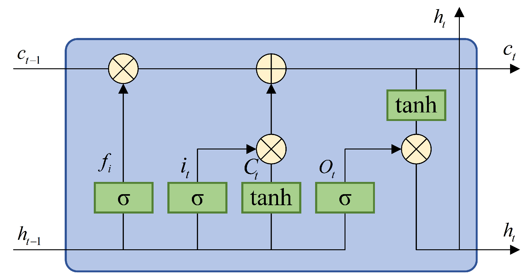
Long short-term memory (LSTM) [35] is a class of neural networks with memory capabilities, designed to handle sequential data, and its structure is illustrated in Figure 5. It is capable of leveraging hidden states to capture temporal information in sequential data. The core of LSTM lies in its memory cell state, which uses a gating mechanism to determine which information should be retained, updated, or discarded. This mechanism mainly includes the forget gate $\mathit{f}$, the input gate $\mathit{i}$, and the output gate $\mathit{e}$. The basic formulas are as follows:

$$\left\{\begin{array}{c}{\mathit{c}}_t={\mathit{f}}_t\odot {\mathit{C}}_{t-1}+{\mathit{i}}_t\odot {\overline{\mathit{c}}}_t\hfill \\ {\mathit{h}}_t={\mathit{e}}_t\odot tanh\left({\mathit{C}}_t\right)\hfill \\ {\overline{\mathit{c}}}_t=tanh\left({\mathit{W}}_{cs}{\mathit{s}}_t+{\mathit{W}}_{ch}{\mathit{h}}_{t-1}+{\mathit{b}}_c\right)\hfill \\ {\mathit{f}}_t=\sigma \left({\mathit{W}}_{fs}{\mathit{s}}_t+{\mathit{W}}_{ff}{\mathit{h}}_{t-1}+{\mathit{b}}_f\right)\hfill \\ {\mathit{i}}_{\mathit{t}}=\sigma \left({\mathit{W}}_{is}{\mathit{s}}_t+{\mathit{W}}_{ih}{\mathit{h}}_{t-1}+{\mathit{b}}_i\right)\hfill \\ {\mathit{e}}_t=\sigma \left({\mathit{W}}_{es}{\mathit{s}}_t+{\mathit{W}}_{eh}{\mathit{h}}_{t-1}+{\mathit{b}}_e\right)\hfill \end{array}\right.,$$

(8)

where ${\mathit{W}}_{(·)}$ and ${\mathit{b}}_{(·)}$ are the parameters of the LSTM network.

3. Guidance Law Implementation

3.1. Algorithm Structure Design

Due to the limitations of the seeker, the training environment is modeled as a POMDP, which significantly reduces the performance of the classical PPO algorithm. Additionally, the defender’s detection frequency typically exceeds its guidance frequency, meaning that multiple measurements can be taken within each guidance cycle. Based on these considerations, we incorporate a temporal network into the PPO algorithm’s architecture by adding a shared LSTM layer to capture additional temporal information in the input. By combining observations from m time steps, the network input at the current time step is expanded into a sequence.

$$\begin{array}{c}\hfill y=\left. [ob{s}_{\mathrm{t}-\mathrm{m}},\cdots ,ob{s}_{\mathrm{t}-2},ob{s}_{\mathrm{t}-1},ob{s}_{\mathrm{t}}\right]\end{array}$$

(9)

The LSTM network is capable of extracting valuable information that is hidden in the historical observation sequence and passing this information to subsequent layers, thereby assisting the agent in training its policy. The introduction of the temporal network mitigates the negative effects caused by the partial observability of the environment, thereby improving the generalization capability of the policy network. The actor–critic network structure that we designed is shown in Figure 6.

During the training process, the hidden state in the LSTM network changes according to the observation sequence, capturing the time-varying hidden information within the sequence. The LSTM network receives the current observation $Ob{s}_t$ and the previous hidden state $h_{t-1}$ at each time step t and then outputs the new hidden state $h_t$. This $h_t$ encodes the entire history of observations from the initial state to the current time. Therefore, the policy network makes decisions based on an analysis of the entire historical trajectory. Through its recurrent structure and gating mechanism, the LSTM automatically learns how to extract the most relevant features from the observation sequence to construct a belief vector. In contrast, the multilayer perceptron (MLP) policy does not have hidden layers and can only optimize based on the current observation. Once the training is complete, the weights are frozen, and the MLP-based policy typically underperforms in stochastic tasks compared to recurrent policy. The policy and value function network architecture are as shown in

Table 2. The policy and value function network architecture.

Layer	Policy Network		Value Network
	Units	Activation	Units	Activation
LSTM	32	Relu	Share with policy network
Layer 1	32	Relu	Share with policy network
Layer 2	32	Relu	32	Relu
Output	action_dim	tanh	1	linear

.

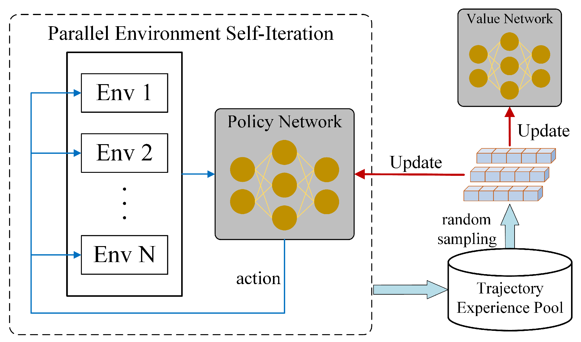
For scenarios involving large exploration spaces, we construct a multi-environment parallel computing framework to guide the update of shared network weights, as shown in Figure 7. The current policy network is executed synchronously in multiple randomly initialized environments to generate differentiated trajectories. This results in a highcoverage sample set under the current policy weights, which is then iteratively optimized through stochastic gradient descent. This approach significantly enhances the stability of policy optimization, effectively suppresses variance oscillations in parameter updates, and accelerates convergence speed.

The flowchart of the algorithm is shown in Figure 8, which extracts observation sequences in the engagement scenario and provides these sequences to the RPPO guidance law framework for training the actor–critic network.

We summarize the proposed method in Algorithm 2.

Algorithm 2 RPPO-based interception guidance law

Input: continuous observation sequence y

Output: normal acceleration $a_{\mathrm{M}}$

1: Initialize the networks’ parameters ${\theta }_0$, value loss weight $\alpha$, and set clipping threshold $ϵ$   2: for n = 1, 2, …, maximum training episode $n_{\max }$ do   3:  Initialize $n_{\mathrm{env}}$ different environments randomly   4:  Compute the learning rate $lr$ and entropy bonus coefficient $\beta$ that decay over time   5:  for t = 1, 2, …, $T_{\max }$ do   6:   for i = 1, 2, …, $n_{\mathrm{env}}$ do   7:    Calculate $a_{\mathrm{M}}$ on policy $\pi \left({\theta }_k\right)$   8:    Update the current environment state   9:   end for 10:   Collect set of partial trajectories $D_t$ from different environments 11:  end for 12:  Divide $D_t$ into continuous sequences of length $n_{len}$ 13:  Compute advantage estimates $\widehat{A}$ 14:  for k = 1, 2, …, maximum RPPO epochs $k_{\max }$ do 15:   Compute loss function $L\left(\theta \right)=L^{\mathrm{CLIP}}\left(\theta \right)+\alpha L^{\mathrm{VF}}\left(\theta \right)+\beta L^{\mathrm{ENT}}\left(\theta \right)$ 16:   Update weights via backpropagation 17:  end for 18: end for

3.2. Implementation Details

In the defender flight process, the defender acquires limited information through its sensors, making it difficult to reflect the overall state of the engagement. As a result, our dynamic model is formulated as a POMDP. The observation space is defined as follows:

$$\begin{array}{c}\hfill obs=\left. [R,{\lambda }_{\mathrm{t}},{\lambda }_{\mathrm{p}},{\dot{\lambda }}_{\mathrm{t}},{\dot{\lambda }}_{\mathrm{p}}\right].\end{array}$$

(10)

We select the relative distance, LOS angle, and LOS angular velocity as the observations. These quantities are relative measurements, which allows for broader applicability. Considering the significant differences in the magnitudes of the observed variables, which may adversely affect the training process, it is necessary to normalize these observations during training to ensure consistency and improve stability.

In Assumption 3, we assume that the velocity is constant and the motion state of the defender is completely controlled by normal acceleration. Consequently, the action space is designed as follows:

$$\begin{array}{c}\hfill a_{\mathrm{M}}=\left. [a_y,a_z\right],a_y,a_z\in \left. [-n_{\mathrm{M}}g,n_{\mathrm{M}}g\right],\end{array}$$

(11)

where $n_{\mathrm{M}}$ represents the maximum overload of the defender. The gravitational acceleration g is taken as $9.81$ m/s². The action space is thus constrained by this overload limit, ensuring that the defender’s trajectory can be effectively controlled within the allowable range of normal accelerations.

The design of the reward function based on the environmental task is critical for the training of agents in DRL. Through our experiments, we have observed that the reward design based on collision triangles imposes strict constraints. However, in our study, the initial launch angle is randomly chosen within a certain range, making it impossible to constrain the LOS angle. Relying solely on the LOS angular velocity fails to achieve convergence. Therefore, a more robust reward function design is required. The proposed reward function is described as Equation (12):

$$\begin{array}{c}\hfill reward=r_{\mathrm{end}}+r_{\mathrm{dis}}+r_{\mathrm{los}}+r_{\mathrm{pre}}\end{array}$$

(12)

Here, $r_{\mathrm{end}}$ represents the terminal reward, as shown in Equation (13). If $R<R_{\mathrm{miss}}$, it indicates a successful interception, and the agent receives a positive reward. Conversely, if the condition is not met, the interception fails, and the agent does not receive any reward.

$$\begin{array}{c}\hfill r_{\mathrm{end}}=\left\{\begin{array}{c}{\beta }_1,R\le R_{\mathrm{miss}}\hfill \\ 0,\mathrm{else}\hfill \end{array}\right.\end{array}$$

(13)

Here, $r_{\mathrm{dis}}$ is the reward designed based on the distance between the defender and the UAV. During its design, the potential-based reward method was referenced, encouraging the defender to approach the UAV and receive a positive reward.

$$\begin{array}{c}\hfill r_{\mathrm{dis}}={\displaystyle \frac{{\beta }_2}{|R_0-R|+R_0}}\Delta R\end{array}$$

(14)

and

$$\begin{array}{c}\hfill \Delta R=R_{t-1}-R_t\end{array}$$

(15)

Here, $r_{\mathrm{los}}$ is the reward related to the LOS angular velocity. The classic parallel approach method was employed, with the goal of converging the LOS angular velocity to zero during the interception process. Additionally, a logarithmic function related to time was designed to constrain the LOS angular velocity. This allows the defender to experience larger changes in LOS angular velocity during the early stages of the environment, but in the later stages of each simulation, we encourage the LOS angular velocity to remain near zero without significant fluctuations. This approach effectively imposes an indirect constraint on the defender’s trajectory, permitting maneuvering during the initial phase to quickly form a collision triangle with the UAV, thereby constraining the trajectory overload at the front end. This resolves the issue of uneven overload distribution in the defender’s trajectory.

$$\begin{array}{c}\hfill r_{\mathrm{los}}=-{\beta }_3\left(\left|{\dot{\lambda }}_{\mathrm{t}}\right|+\left|{\dot{\lambda }}_{\mathrm{p}}\right|\right)ln({\beta }_{4}t+1)\end{array}$$

(16)

Here, $r_{\mathrm{pre}}$ represents the reward based on the prediction information. In our experiments, we found that using only the three aforementioned rewards did not result in good convergence. This is because in a three-dimensional space, the agent explores a large space and requires the more directive reward to guide convergence effectively.

$$\begin{array}{c}\hfill r_{\mathrm{pre}}=-{\beta }_5\left(\left|V_{\mathrm{Ty}}-V_{\mathrm{My}}\right|+\left|V_{\mathrm{Tz}}-V_{\mathrm{Mz}}\right|\right)\end{array}$$

(17)

We consider utilizing historical observation data to predict the motion information of the UAV, taking the LOS y-direction as an example, as shown in Equation (18).

$$\left\{\begin{array}{c}{V}_{\mathrm{Ty}}\left(t-1\right)=V_{\mathrm{My}}\left(t-1\right)+{\dot{\lambda }}_{\mathrm{t}}\left(t-1\right)R_{\mathrm{t}-1}\hfill \\ V_{\mathrm{Ty}}\left(t\right)=V_{\mathrm{My}}\left(t\right)+{\dot{\lambda }}_{\mathrm{t}}\left(t\right)R_{\mathrm{t}}\hfill \\ \Delta V_{\mathrm{Ty}}=V_{\mathrm{Ty}}\left(t\right)-V_{\mathrm{Ty}}\left(t-1\right)\hfill \\ {\displaystyle V_{\mathrm{Ty}}\approx V_{\mathrm{Ty}}\left(t\right)+\frac{\Delta V_{\mathrm{Ty}}}{\Delta t}t}\hfill \end{array}\right.$$

(18)

The UAV velocity is calculated based on the observations at the current and previous time steps. Considering the short integration time step used, we neglect the UAV’s acceleration change within a single time step, and the velocity increment is added to the next time step to make a rough prediction of the UAV’s future motion. This prediction is updated over time, is simple and efficient, and avoids error accumulation. After obtaining the predicted UAV velocity, based on the parallel approach method, we aim for the defender’s and UAV’s velocities in the LOS normal direction to be as equal as possible, and thus, we design the predictive reward.

4. Numerical Simulation

4.1. Training Process

As described in Section 2.2, the initial states of both the defender and the UAV are randomly initialized during training to ensure the universality of the trained strategy. Considering the defender’s detection frequency, a fourth-order Runge–Kutta integrator with a step size of $0.01$ $\mathrm{s}$ is employed in the experiment. The value of m in Equation (9) is set to 8.

Table 3. Network hyperparameters.

Parameter	Value	Parameter	Value
${\beta }_1$	50	$ϵ$	0.2
${\beta }_2$	80	$\alpha$	0.2
${\beta }_3$	−0.04	$n_{\mathrm{env}}$	16
${\beta }_4$	0.2	$k_{\max }$	8
${\beta }_5$	−0.05	$T_{\max }$	1024
$R_0$	4000	$n_{\mathrm{M}}$	10
$lr$	0.0003 → 0.0001	$\beta$	0.001 → 0.0001

lists all the hyperparameters used in the training process.

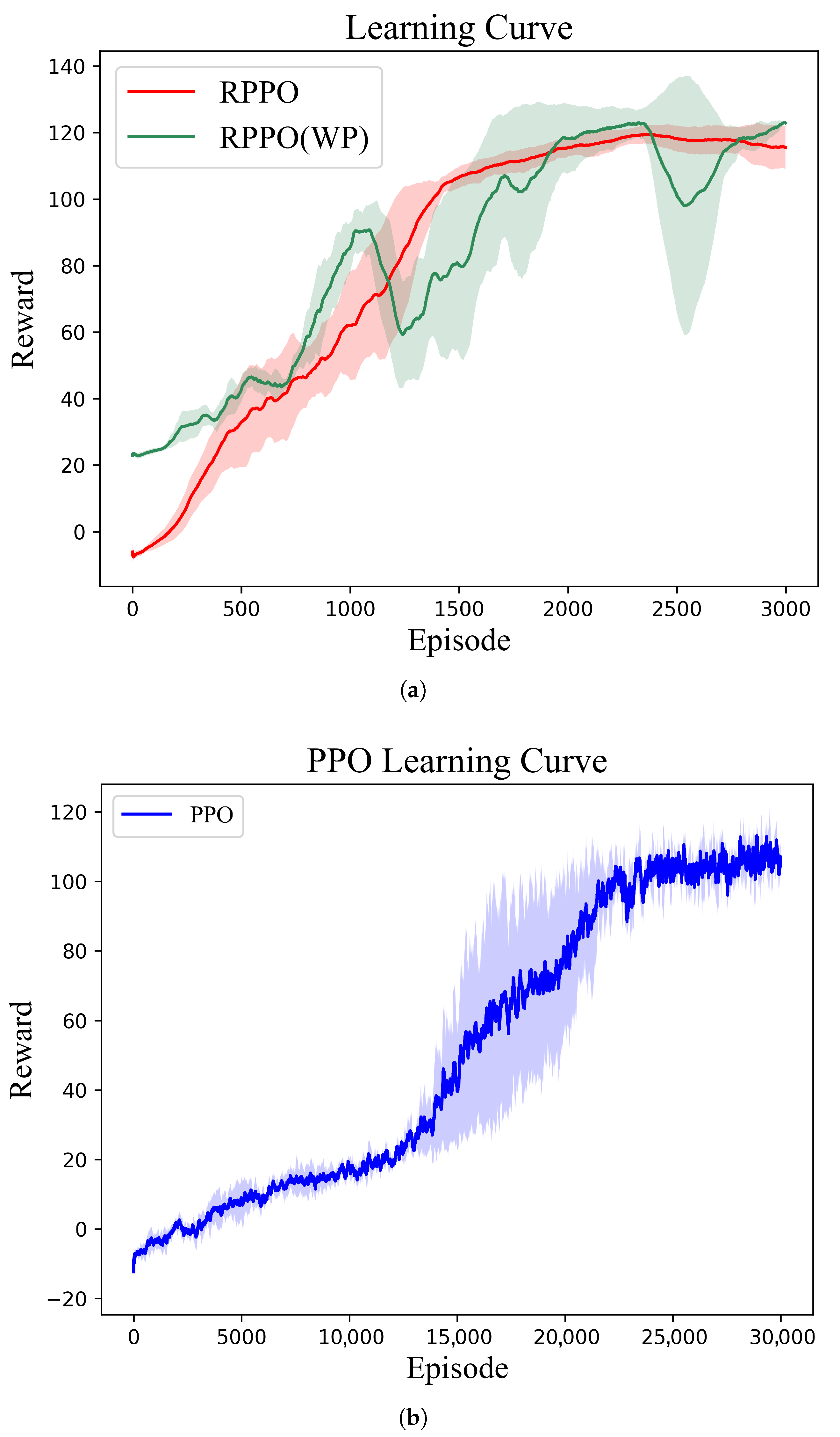
The proposed RPPO guidance law was trained in the above random scenario, and the learning curve after 3000 training episodes is shown in Figure 9a. It is evident that in the first 1500 episodes of training, the average reward of RPPO gradually increased, after which it slowly rose and stabilized, indicating that the trained policy network had converged.

We also employed the classical PPO algorithm for training, with the learning curve being shown in Figure 9b. The classical PPO method exhibits low learning efficiency in complex environments; it takes approximately 25,000 episodes to converge to a suboptimal solution, with the reward curve being unable to continue rising to the maximum. In contrast, our proposed RPPO method employs a multi-environment parallel computing framework that performs simultaneous iterations in diverse environments, thereby improving data utilization and accelerating training. Moreover, incorporating a recurrent network into the actor–critic architecture mitigates the impact of partial observability, enabling the agent to learn a superior strategy.

Furthermore, we conducted tests on the predictive reward term. As shown in Figure 9a, when all other conditions remain unchanged, but the reward does not include predictive information, the reward curve exhibits greater fluctuations and converges more slowly. This highlights the crucial role of the predictive term in the reward design, which effectively guides the network to converge rapidly and learn a good strategy in sparse reward scenarios.

In conclusion, the proposed RPPO algorithm framework enhances training speed, alleviates the negative effects of partial observability, and improves the stability of the training process.

4.2. Tests in the Training Scenario

To verify the performance of our proposed guidance law based on the RPPO framework, we conducted the following simulation tests on the trained model:

We first conducted tests in the environment introduced in Section 2, comparing the APNG law methods as shown in Equation (19). Among them, $K_{\mathrm{APN}}=3$, ${\widehat{a}}_{\mathrm{T}}$ denotes the estimation of defender acceleration.

$$\begin{array}{c}\hfill a_{\mathrm{APN}}=K_{\mathrm{APN}}\dot{R}\dot{\lambda }+{\displaystyle \frac{1}{2}}{K}_{\mathrm{APN}}{\widehat{a}}_{\mathrm{T}}\end{array}$$

(19)

We conducted 1000 Monte Carlo simulations for each of the different methods, and the results are presented in

Table 4. Comparison of different guidance laws.

Guidance Law	Interception Rate	Miss Distance
		Mean (m)	Variance (m2)
APNG	89.1%	1.3226	0.5658
RPPO	95.3%	1.2935	0.5493

. The results indicate that the proposed RPPO guidance law framework achieves an interception rate of 95.3%, with an average miss distance of 1.2935 m and a miss distance variance of 0.5493 m². Compared to the classical APNG law, the performance of the proposed guidance law has been improved. Under conditions of limited observability and maneuverability, the RPPO guidance law framework is still capable of achieving a high interception rate, demonstrating its practical engineering significance.

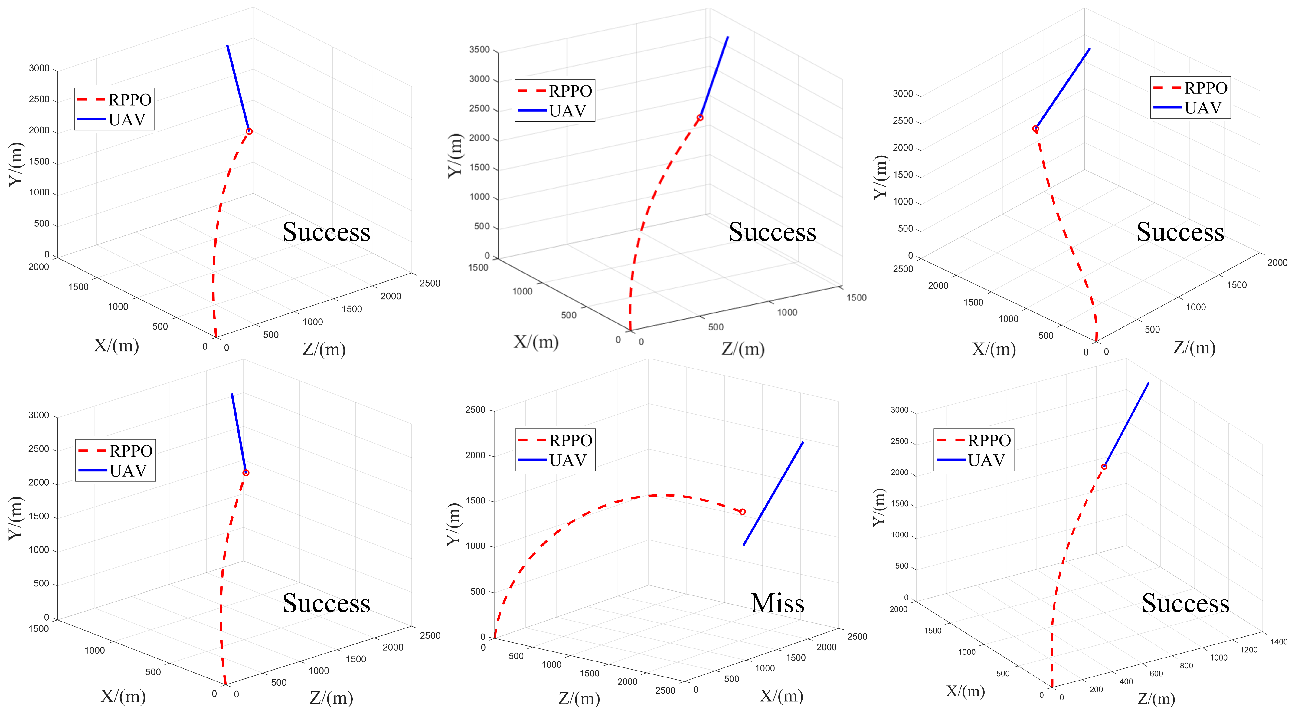
We have visualized a portion of the trajectories, as shown in Figure 10. From the visualization results, it can be seen that the proposed RPPO guidance law framework effectively confines the overload to the front end. If the initial launch angle difference between the defender and the UAV is too large, such that the interception process exceeds the defender’s maneuverability, the defender will be unable to intercept the UAV. In all other scenarios, the defender can effectively intercept the UAV through maneuvering.

Figure 11 illustrates the engagement scenario of the defender and the UAV, including the flight paths of both the defender and the UAV, as well as the defender’s normal acceleration curves. In this scenario, the initial distance $R=3712 \mathrm{m}$, and the LOS angle ${\lambda }_{\mathrm{t}}=39.3^{\circ }$, ${\lambda }_{\mathrm{p}}=45.8^{\circ }$. The RPPO and APNG methods both successfully intercept the UAV, with miss distances of $1.2171$ $\mathrm{m}$ and $2.4570$ $\mathrm{m}$, respectively.

By analyzing the information in Figure 11a,b, it is evident that the guidance law based on the RPPO framework effectively constrains the trajectory overload distribution. This design concentrates the trajectory overload in the initial phase, leaving sufficient margin for subsequent maneuvers. In contrast, traditional guidance laws primarily focus on the overload in the terminal phase, requiring a much higher overload than available, which can easily result in a miss. This clearly demonstrates the effectiveness and necessity of the RPPO-guided law framework design.

4.3. Generalization to Unseen Scenarios

The above tests demonstrate the advantages of the proposed RPPO guidance law framework in the training scenarios. This section will evaluate the adaptability of the trained policy to new scenarios, specifically examining the generalization capability of the policy. During the training process, we only considered the case of a UAV moving at a constant velocity. To further assess the defender’s interception rate when the UAV’s maneuvering mode changes, a new maneuvering mode for the UAV is assigned, as shown in Equation (20).

$$\begin{array}{c}\hfill V_{\mathrm{Tz}}=-100sink\Delta t\end{array}$$

(20)

Here, $\Delta t$ is defined as the unit step size. It means that the UAV is performing a sinusoidal maneuver in the z-axis direction. We also conducted 1000 Monte Carlo simulations, and the results are shown in

Table 5. Generalization comparison of different guidance laws.

Guidance Law	Interception Rate	Miss Distance
		Mean (m)	Variance (m2)
APNG	84.1 %	1.7942	1.0865
RPPO	93.0 %	1.7490	0.9804

. The findings indicate that even in previously untrained scenarios, the policy trained using RPPO exhibits strong generalization capability, with an interception accuracy exceeding that of traditional guidance law algorithms.

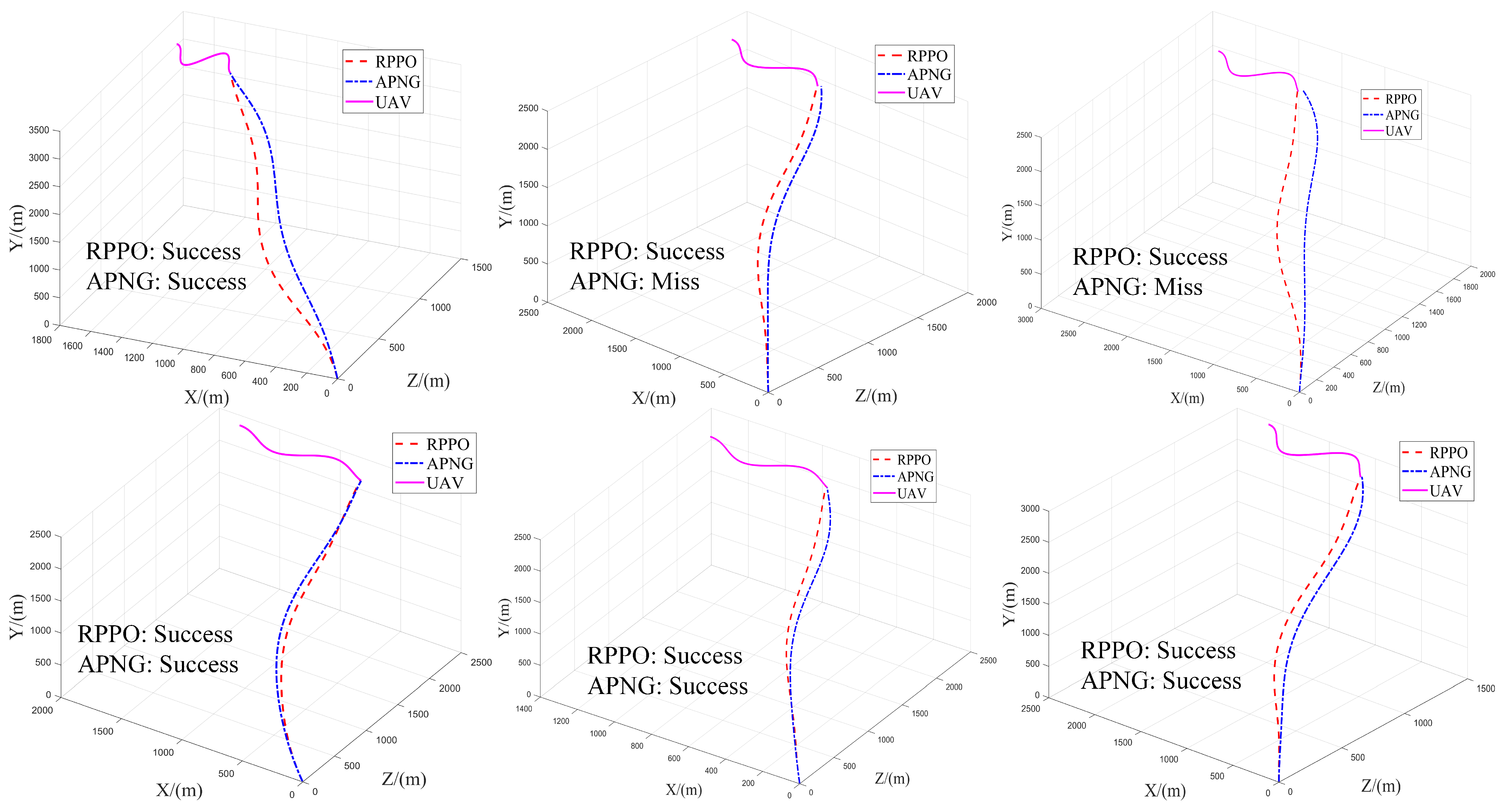
We also visualized some trajectories, as shown in Figure 12. It can be seen from the figure that in the face of the UAV’s complex maneuvers, the RPPO guidance law is still able to intercept the UAV effectively, whereas the APNG method does not handle this situation well.

The reason for the strong generalization ability of the RPPO guidance law framework lies in its focus on the relative relationship between the defender and the UAV during training, while disregarding their individual motions. Additionally, the RPPO guidance law restricts the defender’s maneuvering to the early stage of the trajectory, thereby preserving maneuvering margin for the later stage. This approach allows the low-overload defender to handle the UAV maneuvers better and improves its hit accuracy.

In actual engagement scenarios, UAVs typically adjust their maneuvering strategies based on the level of threat. To simulate this sudden maneuvering behavior, we define the following: When the relative distance between the UAV and the defender is greater than a certain threshold, the UAV will switch its maneuver mode. Specifically, when the relative distance R exceeds 1000 m, the UAV maintains a constant-speed maneuver, as described in Section 4.2. The initial velocity of the UAV is set within the range of 50 m/s to 80 m/s. However, when the relative distance R drops below 1000 m, the UAV switches to a new maneuver mode, performing sinusoidal maneuvers along the Z-axis, while the velocities in the X-axis and Y-axis remain unchanged.

For the scenario described above, we also conducted a Monte Carlo simulation, and the results are presented in

Table 6. Comparison of different guidance laws in scenarios with sudden maneuvering.

Guidance Law	Interception Rate	Miss Distance
		Mean (m)	Variance (m2)
APNG	83.4 %	1.7938	1.0758
RPPO	93.3 %	1.7495	0.9565

. From these results, it can be observed that even in the face of the UAV’s sudden maneuvers, the RPPO guidance law still demonstrates excellent performance.

4.4. Noise Robustness Test

Considering the uncertainties brought by noise in real-world scenarios, the proposed RPPO guidance law is further required to possess robustness. Specifically, Gaussian white noise is added to the observation data, as described in Equation (21),

$$\begin{array}{c}\hfill ob{s}_{\mathrm{noise}}=obs·{\delta }_o\end{array}$$

(21)

where ${\delta }_o\sim N(1,{\sigma }_o^2)$.

The tests are conducted in the scenario presented in Section 4.3, where different values of variance ${\sigma }_o$ are selected to evaluate the interception rate and the miss distance. The variance ${\sigma }_o$ of the environmental noise, which follows a normal distribution, is set to values of 0, 0.1, 0.2, 0.3, 0.4, and 0.5. Figure 13 presents the probability density curves under different variance conditions.

For each noise setting, we performed three independent Monte Carlo runs with 1000 episodes each and reported the averaged results across these runs. The final results are shown in

Table 7. Testing under different variance conditions.

Variance ${\mathit{\sigma }}_{\mathit{o}}$	Guidance Law
	APNG		RPPO
	Interception Rate	Miss Distance (m)	Interception Rate	Miss Distance (m)
${\sigma }_o=0$	84.09%	1.7942	93.02%	1.7490
${\sigma }_o=0.1$	82.77%	1.8328	91.87%	1.7140
${\sigma }_o=0.2$	78.27%	1.9127	91.33%	1.7789
${\sigma }_o=0.3$	72.50%	2.0177	90.37%	1.8066
${\sigma }_o=0.4$	62.17%	2.1479	89.73%	1.8983
${\sigma }_o=0.5$	41.73%	2.2478	87.23%	1.9213

.

Based on the experimental results, the proposed RPPO guidance law demonstrates superior performance compared to the APNG guidance law when exposed to noise with varying levels of variance. In all cases, the RPPO guidance law demonstrates a higher interception rate and a smaller miss distance, indicating stronger robustness against the unknown noise.

4.5. Significance Testing Experiment

We conducted a significance analysis of the above results, and the findings are presented in

Table 8. Significance test results for the RPPO guidance law and the APNG guidance law.

Comparison	t-Value	df	p-Value	Hedges’g	BF10	Significant?
Case 1	2.636	999	8.525 $\times {10}^{-3}$	0.117	1.124	✓
Case 2	9.003	2999	3.800 $\times {10}^{-19}$	0.226	4.624 $\times {10}^{15}$	✓
Case 3	9.998	2999	3.561 $\times {10}^{-23}$	0.246	4.427 $\times {10}^{19}$	✓
Case 4	11.697	2999	6.174 $\times {10}^{-31}$	0.296	2.165 $\times {10}^{27}$	✓
Case 5	13.077	2999	4.828 $\times {10}^{-38}$	0.333	2.455 $\times {10}^{34}$	✓
Case 6	15.852	2999	2.071 $\times {10}^{-54}$	0.405	4.628 $\times {10}^{50}$	✓
Case 7	21.204	2999	4.286 $\times {10}^{-93}$	0.546	1.597 $\times {10}^{89}$	✓

. The analysis indicates that the RPPO guidance law significantly outperforms the APNG guidance law in terms of statistical significance, effect size, and Bayes factor.

Case 1 corresponds to the test results in Section 4.2, Case 2 corresponds to the test results in Section 4.3, and Cases 3 to 7 correspond to the test results in Section 4.4 with variance ${\sigma }_o$ values of 0.1, 0.2, 0.3, 0.4, and 0.5, respectively.

The p-values for all seven cases are much smaller than 0.05, indicating that the differences in each case are statistically significant. For instance, Case 2 achieves a t-value of 9.003 ($p=3.800\times {10}^{-19}$), an effect size of 0.226, and a Bayes Factor of 4.624 $\times {10}^{15}$, demonstrating a very strong difference between the two algorithms. In Cases 3 to 7, as the variance ${\sigma }_o$ increases, the t-value, effect size, and Bayes Factor all gradually increase, especially in Case 6 and Case 7, where very strong differences are observed. These results conclusively highlight the exceptional performance of the RPPO guidance law.

5. Conclusions

To address the challenge of intercepting LSS UAVs with a low-overload defender, we propose the RPPO guidance law framework based on DRL in this paper. We construct a frontal engagement scenario in three-dimensional space and introduce more broad initial launch conditions. Due to the partial observability of the seeker and overload constraints, we propose the RPPO guidance law framework, which introduces a temporal network to extract temporal information from the observation sequence. Additionally, we employ a multi-environment parallel training method to improve data utilization and accelerate the training process. We design a reward function based on velocity prediction and overload constraints, which effectively guides the training to converge rapidly in large exploration spaces while constraining the defender overload. Comparison with the widely used APNG method demonstrates the superior performance of our approach, which also exhibits strong generalization capabilities in new scenarios. Future work will focus on two primary directions: first, integrating actuator dynamics into the reinforcement learning framework to enhance the physical feasibility of commands, and second, exploring complex cooperative engagement strategies within the context of multi-agent reinforcement learning.

References

1. Guo, Y.; Li, X.; Zhang, H.; Cai, M.; He, F. Data-driven method for impact time control based on proportional navigation guidance. J. Guid. Control Dyn. 2020, 43, 955–966. [Google Scholar] [CrossRef]
2. Zarchan, P. Tactical and Strategic Missile Guidance; American Institute of Aeronautics and Astronautics, Inc.: Reston, VA, USA, 2012. [Google Scholar]
3. Quarta, A.A.; Bassetto, M.; Mengali, G.; Salem, K.A.; Palaia, G. Optimal guidance laws for diffractive solar sails with Littrow transmission grating. Aerosp. Sci. Technol. 2024, 145, 108860. [Google Scholar] [CrossRef]
4. Ming, C.; Wang, X. Nonsingular terminal sliding mode control-based prescribed performance guidance law with impact angle constraints. Int. J. Control Autom. Syst. 2022, 20, 715–726. [Google Scholar] [CrossRef]
5. Zhang, B.; Zhou, D. Optimal predictive sliding-mode guidance law for intercepting near-space hypersonic maneuvering target. Chin. J. Aeronaut. 2022, 35, 320–331. [Google Scholar] [CrossRef]
6. Asher, R.B.; Matuszewski, J.P. Optimal guidance with maneuvering targets. J. Spacecr. Rocket. 1974, 11, 204–206. [Google Scholar] [CrossRef]
7. Dun, X.; Li, J.; Cai, J. Optimal guidance law for intercepting high-speed maneuvering targets. J. Natl. Univ. Def. Technol. 2018, 1, 176–182. [Google Scholar]
8. Kim, Y.W.; Kim, B.; Lee, C.H.; He, S. A Unified Formulation of Optimal Guidance-to-Collision Law for Accelerating and Decelerating Targets. Chin. J. Aeronaut. 2022, 35, 40–54. [Google Scholar] [CrossRef]
9. Shima, T. Intercept-angle guidance. J. Guid. Control Dyn. 2011, 34, 484–492. [Google Scholar] [CrossRef]
10. Zheng, Z.; Li, J.; Feroskhan, M. Three-Dimensional Terminal Angle Constraint Guidance Law with Class K Function-Based Adaptive Sliding Mode Control. Aerosp. Sci. Technol. 2024, 147, 109005. [Google Scholar] [CrossRef]
11. Watkins, C.J.C.H. Learning from Delayed Reward. Ph.D. Thesis, King’s College, University of Cambridge, Cambridge, UK, 1989. [Google Scholar]
12. Mnih, V.; Kavukcuoglu, K.; Silver, D.; Rusu, A.A.; Veness, J.; Bellemare, M.G.; Graves, A.; Riedmiller, M.; Fidjeland, A.K.; Ostrovski, G.; et al. Human-level control through deep reinforcement learning. Nature 2015, 518, 529–533. [Google Scholar] [CrossRef]
13. Vinyals, O.; Babuschkin, I.; Czarnecki, W.; Mathieu, M.; Dudzik, A.; Chung, J.; Choi, D.; Powell, R.; Ewalds, T.; Georgiev, P.; et al. Grandmaster level in StarCraft II using multi-agent reinforcement learning. Nature 2019, 575, 350–354. [Google Scholar] [CrossRef]
14. Choi, J.; Kim, H.M.; Hwang, H.J.; Kim, Y.D.; Kim, C.O. Modular reinforcement learning for autonomous UAV flight control. Drones 2023, 7, 418. [Google Scholar] [CrossRef]
15. Wang, M.; Jia, S.; Niu, Y.; Liu, Y.; Yan, C.; Wang, C. Agile Flights Through a Moving Narrow Gap for Quadrotors Using Adaptive Curriculum Learning. IEEE Trans. Intell. Veh. 2024, 9, 6936–6949. [Google Scholar] [CrossRef]
16. Li, J.; Li, J.; Yang, G.; Yang, L.; Chi, H.; Yang, L. Applications of Large Language Models and Multimodal Large Models in Autonomous Driving: A Comprehensive Review. Drones 2025, 9, 238. [Google Scholar] [CrossRef]
17. Fan, J.; Dou, D.; Ji, Y. Impact-angle constraint guidance and control strategies based on deep reinforcement learning. Aerospace 2023, 10, 954. [Google Scholar] [CrossRef]
18. Xi, A.; Cai, Y. Deep Reinforcement Learning-Based Differential Game Guidance Law against Maneuvering Evaders. Aerospace 2024, 11, 558. [Google Scholar] [CrossRef]
19. Ladosz, P.; Weng, L.; Kim, M.; Oh, H. Exploration in deep reinforcement learning: A survey. Inf. Fusion 2022, 85, 1–22. [Google Scholar] [CrossRef]
20. Hu, Z.; Yi, W.; Xiao, L. Deep Reinforcement Learning-Based Impact Angle-Constrained Adaptive Guidance Law. Mathematics 2025, 13, 987. [Google Scholar] [CrossRef]
21. Fujimoto, S.; Hoof, H.; Meger, D. Addressing function approximation error in actor-critic methods. In Proceedings of the International Conference on Machine Learning, PMLR, Stockholm, Sweden, 10–15 July 2018; pp. 1587–1596. [Google Scholar]
22. Gaudet, B.; Furfaro, R.; Linares, R. Reinforcement Learning for Angle-Only Intercept Guidance of Maneuvering Targets. Aerosp. Sci. Technol. 2020, 99, 105746. [Google Scholar] [CrossRef]
23. Scorsoglio, A.; D’Ambrosio, A.; Ghilardi, L.; Gaudet, B.; Curti, F.; Furfaro, R. Image-based deep reinforcement meta-learning for autonomous lunar landing. J. Spacecr. Rocket. 2022, 59, 153–165. [Google Scholar] [CrossRef]
24. Gaudet, B.; Linares, R.; Furfaro, R. Terminal adaptive guidance via reinforcement meta-learning: Applications to autonomous asteroid close-proximity operations. Acta Astronaut. 2020, 171, 1–13. [Google Scholar] [CrossRef]
25. Gaudet, B.; Linares, R.; Furfaro, R. Six degree-of-freedom body-fixed hovering over unmapped asteroids via LIDAR altimetry and reinforcement meta-learning. Acta Astronaut. 2020, 172, 90–99. [Google Scholar] [CrossRef]
26. Qiu, X.; Lai, P.; Gao, C.; Jing, W. Recorded Recurrent Deep Reinforcement Learning Guidance Laws for Intercepting Endoatmospheric Maneuvering Missiles. Def. Technol. 2024, 31, 457–470. [Google Scholar] [CrossRef]
27. Qiu, X.; Gao, C.; Jing, W. Deep Reinforcement Learning Guidance Law for Intercepting Endo atmospheric Maneuvering Targets. J. Astronaut. 2022, 43, 685. [Google Scholar]
28. Wang, X.; Deng, Y.; Cai, Y.; Jiang, H. Deep Recurrent Reinforcement Learning for Intercept Guidance Law under Partial Observability. Appl. Artif. Intell. 2024, 38, 2355023. [Google Scholar] [CrossRef]
29. He, S.; Shin, H.S.; Tsourdos, A. Computational missile guidance: A deep reinforcement learning approach. J. Aerosp. Inf. Syst. 2021, 18, 571–582. [Google Scholar] [CrossRef]
30. Liu, Z.; Wang, J.; He, S.; Shin, H.S.; Tsourdos, A. Learning prediction-correction guidance for impact time control. Aerosp. Sci. Technol. 2021, 119, 107187. [Google Scholar] [CrossRef]
31. Cao, W.; Huang, J.; Chang, S. Data-Driven-Method-Based Guidance Law for Impact Time and Angle Constraints. Aerospace 2024, 11, 540. [Google Scholar] [CrossRef]
32. Song, T.L.; Um, T.Y. Practical guidance for homing missiles with bearings-only measurements. IEEE Trans. Aerosp. Electron. Syst. 1996, 32, 434–443. [Google Scholar] [CrossRef]
33. Sutton, R.; Barto, A. Reinforcement Learning: An Introduction. IEEE Trans. Neural Netw. 1998, 9, 1054. [Google Scholar] [CrossRef]
34. Schulman, J.; Wolski, F.; Dhariwal, P.; Radford, A.; Klimov, O. Proximal policy optimization algorithms. arXiv 2017, arXiv:1707.06347. [Google Scholar] [CrossRef]
35. Shi, X.; Chen, Z.; Wang, H.; Yeung, D.Y.; Wong, W.K.; Woo, W.c. Convolutional LSTM network: A machine learning approach for precipitation nowcasting. In Advances in Neural Information Processing Systems; NeurIPS: San Diego, CA, USA, 2015; Volume 28. [Google Scholar]
Figure 1. Assumption of the collision triangle in the two-dimensional plane.
Aerospace 12 00968 g001
Figure 2. The three-dimensional engagement scenario. The defender is launched from the origin, while the UAV approaches from a distant location.
Aerospace 12 00968 g002
Figure 3. Interaction between agent and environment.
Aerospace 12 00968 g003
Figure 4. PPO algorithm flow diagram.
Aerospace 12 00968 g004
Figure 5. The structural diagram of the LSTM module.
Aerospace 12 00968 g005
Figure 6. The RPPO algorithm’s actor–critic network structure. The input is the current observation sequence y. The policy network branch outputs the actions, while the value network branch outputs the corresponding value.
Aerospace 12 00968 g006
Figure 7. The multi-environment parallel computing framework. Multiple distinct environments run in parallel and jointly update the policy network and the value network.
Aerospace 12 00968 g007
Figure 8. The flowchart of the RPPO guidance law framework. The observation sequence is calculated through an engagement scenario and then transmitted to the actor–critic network.
Aerospace 12 00968 g008
Figure 9. Learning curve. (a) Learning curve of the proposed RPPO method. The label RPPO represents the learning curve of the proposed guidance law method, while the label RPPO (WP) represents the learning curve of the RPPO method without the reward prediction term r pre . (b) Learning curve of the classical PPO method.
Aerospace 12 00968 g009
Figure 10. Visualization of the defender–UAV trajectory. The UAV employs a constant value maneuver, while the defender utilizes the RPPO guidance law for interception. The label “success” means that the defender successfully intercepts the UAV, while the label “miss” means a failure in interception.
Aerospace 12 00968 g010
Figure 11. Defender–UAV interception engagement scenario. (a) Engagement trajectory. (b) Ballistic overload distribution.
Aerospace 12 00968 g011
Figure 12. Visualization of the defender–UAV trajectory. The UAV employs a sinusoidal value maneuver. The label “success” means that the defender successfully intercepts the UAV, while the label “miss” means a failure in interception.
Aerospace 12 00968 g012
Figure 13. Normal distribution δ o curves with different values of σ o .
Aerospace 12 00968 g013