Identifying the Location of Dynamic Load Using a Region’s Asymptotic Approximation

Abstract

Since it is difficult to obtain the positions of dynamic loads on structures, this paper suggests a new method to identify the locations of dynamic loads step-by-step based on the correlation coefficients of dynamic responses. First, a recognition model for dynamic load position based on a finite-element scheme is established, with the finite-element domain divided into several regions. Second, virtual loads are applied at the central points of these regions, and acceleration responses are calculated at the sensor measurement points. Third, the maximum correlation coefficient between the calculational and measured accelerations is obtained, and the dynamic load is located in the region with the virtual load corresponding to the maximum correlation coefficient. Finally, this region is continuously subdivided with the refined mesh until the dynamic load is pinpointed in a sufficiently small area. Different virtual load construction methods are proposed according to different types of loads. The frequency response function, unresolvable for the actual problem due to the unknown location of the real dynamic load, can be transformed into a solvable form, involving only known points. This transformation simplifies the analytical process, making it more efficient and applicable to analysis of the dynamic behavior of the system. The identification of the dynamic load position in the entire structure is then transformed into a sub-region approach, focusing on the area where the dynamic load acts. Simulations for case studies are conducted to demonstrate that the proposed method can effectively identify positions of single and multiple dynamic loads. The correctness of the theory and simulation model is verified with experiments. Compared to recent methods that use machine learning and neural networks to identify positions of dynamic loads, the approach proposed in this paper avoids the heavy computational cost and time required for data training.

1. Introduction

Dynamic load identification is a type of inverse dynamic problem, where inputs (loads) are identified using outputs (responses) and structural parameters in a structural-dynamic system. In practical engineering applications, direct measurements of dynamic load position are often difficult. However, identification of these loads is crucial in various scenarios, such as moving loads on bridges [1] or external in-flight loads on aircrafts. Accurate identification of dynamic load locations is essential for structural design and health monitoring [2]. In the field of nano mechanics [3], the solution of such inverse problems is also crucial. Since the development of dynamic load identification methods for military applications in 1970 [4], various techniques have been introduced. Among them, the two main types of methods are the following: (i) The time–domain methods [5], which include the direct integration method [6], iterative method, and Green’s function method, and the (ii) frequency–domain methods [7], which include the direct inverse method and the inverse virtual excitation method. The latter methods apply a Fourier transform to the time–domain signal to obtain the amplitude–frequency characteristic curve. This method requires sufficient structural response data for accurate results and is, therefore, primarily suited for identification of long-duration loads. In contrast, the time–domain methods focus on identification of loads based on the convolution relationship between external loads and dynamic responses.

Since the beginning of the 21st century, with the continuous integration of dynamic load identification methods with signal processing, Kalman filtering, neural networks, and other techniques, such as data-driven approaches, principal-component analysis, and stochastic system identification were developed. Li et al. [8] used the inverse finite-element (FE) method to reconstruct the displacement field from discrete response data and then applied interpolation of the radial basis function to obtain a continuous displacement field, which was subsequently used to identify the distributed dynamic loads on a thin plate. Wang et al. [9] proposed a hybrid model combined with a data-driven approach and enhanced the Kalman filtering algorithm to accurately identify dynamic loads even for limited training data, significant noise interference, and non-zero initial conditions. Prawin [10] introduced an online input-force time-history reconstruction algorithm using Dynamic Principal Component Analysis (DPCA). Unlike conventional identification methods, this approach does not require FE discretization of the structure, thus eliminating errors associated with physical modeling. Zhang et al. [11] proposed a method that uses a Bidirectional Long Short-Term Memory (BiLSTM) network model to establish the mapping relationship between the vertical deflection of a bridge and vehicle loads, thereby enabling vehicle load identification. Wang [12] introduced a wavelet-transform-based method for the structural parameter matrix and performed the uncertainty propagation analysis for uncertain variables using the interval analysis of Taylor series expansions, achieving dynamic load identification for multi-source uncertain systems. Meanwhile, with the development of computation capabilities and neural networks, methods for dynamic load identification using deep regression adaptation networks [13], gated convolutional neural networks [14], and deep recurrent neural networks [15] became increasingly prevalent.

The methods mentioned above primarily focus on the identification of distributed dynamic loads or dynamic loads with known positions, while research on the identification of load positions is still relatively limited. Current methods used to identify positions of dynamic loads mainly include exhaustive search, triangulation, time-series inversion, and reference database employing. The exhaustive search method involves obtaining structural vibration information under the influence of loads from numerous measurement points and identifying the load positions with excitation point traversal and numerical optimization algorithms. Zhang [16] established a convolution relationship between the response and the external loads based on structural system parameters, and used a separation of variables algorithm to extract load information from the impulse response function matrix. However, the exhaustive search method often requires the collection of a large amount of data, leading to high costs for load position identification, and also presents certain challenges in data processing. The triangulation method utilizes the mathematical relationship between the impact point, wave velocity, and the time it takes for the shock wave to reach different measurement points. This approach treats the dynamic load location identification problem as a nonlinear mathematical problem involving the geometric relationship between the sensors and the shock wave [17]. Zhao et al. [18] proposed and validated an integrated collision localization scheme that uses the arrival time of signals received by dynamic strain gauges. This method combines triangulation with hybrid particle swarm optimization and genetic algorithms to reconstruct the location of impact loads. Jang [19] enhanced this approach by training a neural network to improve the estimation accuracy of the signal’s propagation distance. However, the triangulation method relies on the assumption that the shock wave’s velocity in different propagation directions is either known or the same, which makes it difficult to achieve high-precision localization for composite materials subjected to low-velocity impacts. The time-series inversion method was initially applied to sound-source localization and later adapted to address dynamic load localization problems [20]. Building on this approach, Ciampa [21] proposed an image-processing method for impact-excitation reconstruction, specifically for composite structures. This method combines the response data with Green’s functions to achieve the reconstruction of both the spatial and temporal domains of impact loads. While the time-series inversion method is widely used in dynamic load localization research, it requires sufficient and high-quality response data to ensure precise localization of the impact load. The reference database method (RDM) estimates the location of an arbitrary random impact load by training on a grid of reference signals containing information for different impact signals and selecting the most similar reference signal. Liu et al. [22] combined the RDM with a random fractal search algorithm for impact load localization. However, the RDM requires significant time to collect dense training points from the monitored area in order to establish the reference database. This means that the accuracy of the method’s localization heavily depends on the number of training points, and it incurs substantial time costs. In addition, other methods such as frequency response function reconstruction [23], neural networks [24,25], and support vector machines [26] were also used to identify dynamic load locations.

The studies discussed above explore various methods to locate dynamic loads in structures, but accurate identification of load positions in structures often requires their division into a fine FM mesh (Yan et al. [27] identified the position of dynamic load on thin plates by establishing a finite-element model containing 10,240 grids, and Liu et al. [28] identified the positions of dynamic loads on plates by constructing a transfer matrix H with a size of 1024 × 27,648), leading to intensive and time-consuming computations. To address this computational challenge, this study draws on the method of inverse problem solving through different vibration responses in nanomaterials [29] to propose a more efficient method, that is, dividing the structure into several parts and computing for key points in each part. Once an optimal part is identified, it can be further refined for greater accuracy. This method combines FM analysis with the correlation coefficient, enabling step-by-step identification of the dynamic load location when the number of dynamic loads is known and their positions are not too close to each other. The first part of the paper details the calculation of correlation coefficients for structural acceleration responses, the model for step-by-step identification, and the construction of virtual loads. The second section presents numerical simulation validations of the identification of single-point and multi-point loads under varying noise levels (5%, 10%) and sensor quantities (4, 9). The third part experimentally confirms the method’s accuracy by identifying dynamic loads on a thin plate.

2. Theoretical Model of Dynamic Load Position Recognition

2.1. Structural Finite-Element Mode

For real-life engineering structures, the structural-dynamics model is very complicated, so it is difficult to derive theoretical formulae. For large complex structures, an FM model of dynamics is established:

$$\left[M\right]\left\{\ddot{u}(t)\right\}+\left[C\right]\left\{\dot{u}(t)\right\}+\left[K\right]\left\{u(t)\right\}=\left\{f(t)\right\},$$

(1)

where $\left[M\right]$ is the mass matrix of the structure, $\left[C\right]$ is the damping matrix, $\left[K\right]$ is the stiffness matrix, $\left\{f\left(t\right)\right\}$ is the dynamic load vector, and $\left\{u\left(t\right)\right\}$, $\left\{\dot{u}\left(t\right)\right\},$ and $\left\{\ddot{u}\left(t\right)\right\}$ are the displacement, velocity, and acceleration vectors, respectively.

In the frequency domain, the structural acceleration response can be written as

$$\left\{\ddot{u}\right\}=\left[H\right]\left\{F\right\},$$

(2)

where $\left\{\ddot{u}\right\}$ is the acceleration response vector, $\left[H\right]$ is the frequence-response-function (FRF) matrix of acceleration, and $\left\{F\right\}$ is the excitation vector.

When there are multiple exciting loads $F_1,F_2,\cdots ,F_k$, Equation (2) can be expressed as

$$\left[\begin{array}{c}{\ddot{u}}_1\\ {\ddot{u}}_2\\ ⋮\\ {\ddot{u}}_i\end{array}\right]=\left[\begin{array}{cccc}{H}_{11}& H_{12}& \cdots & H_{1j}\\ H_{21}& H_{22}& \cdots & H_{2j}\\ ⋮& ⋮& \ddots & ⋮\\ H_{i1}& H_{i2}& \cdots & H_{ij}\end{array}\right]\left\{\begin{array}{c}\begin{array}{c}0\\ F_1\\ F_2\\ ⋮\end{array}\\ F_k\\ ⋮\\ 0\end{array}\right\},$$

(3)

Here, ${\ddot{u}}_i$ is the acceleration response at the node i under the load, and $H_{ij}$ is the acceleration FRF between the excitation position j and the dynamic response position i.

2.2. Acceleration Correlation Coefficient

Under the harmonic excitation $F=A\sin \left(\omega t+\theta \right)$, the acceleration response of the system can be expressed as

$$\ddot{u}(t)=\left|H\right|A\sin (\omega t+\theta +\varphi (H)),$$

(4)

where $\left|H\right|$ and $\varphi (H)$ are the amplitude and phase of the acceleration FRF, and $A,\omega$ and $\theta$ are the amplitude, frequency, and phase of the exciting force, respectively.

In engineering practice, the acceleration response is often measured as a set of discrete time–domain signals by a detector. For the m groups of acceleration response data $[{\ddot{u}}_1],[{\ddot{u}}_2]\cdots [{\ddot{u}}_m]$, it is assumed that the time discretization interval is $\Delta \mathrm{t}$ and the number of discrete time intervals is n. The specific form is given in Equation (5).

$$\left\{\begin{array}{c}[{\ddot{u}}_1]=[{\ddot{u}}_{11},{\ddot{u}}_{12}\cdots {\ddot{u}}_{1n}]\\ ⋮\\ [{\ddot{u}}_m]=[{\ddot{u}}_{m1},{\ddot{u}}_{m2}\cdots {\ddot{u}}_{mn}]\end{array}\right.,$$

(5)

$${\ddot{u}}_{\alpha \beta }={\ddot{u}}_{\alpha }(\beta \cdot \Delta \mathrm{t}) (1\le \alpha \le m,1\le \beta \le n),$$

(6)

Taking $[{\ddot{u}}_1]$ and $[{\ddot{u}}_2]$ as examples, the calculation formulas for the correlation coefficients of these two sets of discrete acceleration data are provided below.

$$r_{12}={\displaystyle \frac{{\displaystyle \sum _{i=1}^n({\ddot{u}}_{1n}-{\overline{\ddot{u}}}_1)({\ddot{u}}_{2n}-{\overline{\ddot{u}}}_2)}}{\sqrt{{\displaystyle \sum _{i=1}^n{({\ddot{u}}_{1n}-{\overline{\ddot{u}}}_1)}^2{({\ddot{u}}_{2n}-{\overline{\ddot{u}}}_2)}^2}}}},$$

(7)

Among them

$${\overline{\ddot{u}}}_1={\displaystyle \sum _{i=1}^n\frac{1}{n}}{\ddot{u}}_{1i} , {\overline{\ddot{u}}}_2={\displaystyle \sum _{i=1}^n\frac{1}{n}}{\ddot{u}}_{2i},$$

(8)

When the value range of $r_{12}$ is $[-1,1]$, the value range of $|r_{12}|$ is $[0,1]$. When $|r_{12}|\to 0$, the correlation between the two sets of acceleration data is weak, and when $|r_{12}|\to 1$, the correlation is strong. As the identification range of the measured structure gradually narrows, the correlation coefficient of the acceleration responses becomes increasingly close. Additionally, adding noise to the acceleration responses reduces the correlation coefficient. Therefore, to facilitate the observation of the correlation coefficients in the identification range, correlation metric $M_{12}$ is used to reflect the degree of correlation between the acceleration responses. The calculation formula for $M_{12}$ is as follows:

$$M_{12}=\left|\lg (1-\left|r_{12}\right|)\right|,$$

(9)

When there is more than one correlation coefficient, the average of multiple correlation coefficients is used as the overall acceleration response correlation coefficient to calculate the correlation metric M. Using the m sets of discrete acceleration response data mentioned above as an example, the correlation coefficients between the second through the m-th sets of acceleration responses and the first set of acceleration responses $[{\ddot{u}}_1]$ are calculated, and their average $|r|$ is taken as the overall correlation coefficient. The formula for calculating the overall acceleration response correlation coefficient and the acceleration response correlation metric M is shown below:

$$|r|={\displaystyle \frac{1}{m-1}}{\displaystyle \sum _{j=2}^m|r_{1j}|},$$

(10)

$$M=\left|\lg (1-\left|r\right|)\right|,$$

(11)

2.3. Identification Model of Dynamic Load Position

In the process of identification of dynamic loads at known positions, the dynamic responses and their positions are known quantities, usually obtained by measurement. The dynamic characteristics of the structure are known, that is, the FRF H between the excitation point and the response point is a known quantity, and the formula for the solution of the dynamic load in the frequency domain can be obtained from Equations (2) and (3):

$$[F]={[\tilde{H}]}^{+}\left\{\ddot{u}\right\},$$

(12)

Equation (12) is the recognition model of the dynamic load when the position is known, where $\left[F\right]$ is the dynamic load vector, ${\left[\tilde{H}\right]}^{+}$ is the generalized inverse of the acceleration FRF matrix, and $\left\{\ddot{u}\right\}$ is the dynamic response vector.

Take a two-dimensional flat plate as an example, when the position of the dynamic load is unknown, set as (x,y), the dynamic response $\left\{\ddot{u}\right\}$ in Equation (12) is a known quantity usually measured directly by an acceleration sensor, and the FRF between the excitation position and dynamic response position is an unknown quantity containing the unknown position function, written as $\left[\tilde{H}\left(x,y\right)\right]$. Then, Equation (12) is an equation containing variables x, y:

$$[F]={[\tilde{H}(x,y)]}^{+}\left\{\ddot{u}\right\},$$

(13)

Among them, the unknown quantities (x,y) are generated due to the unknown position of the actual dynamic load.

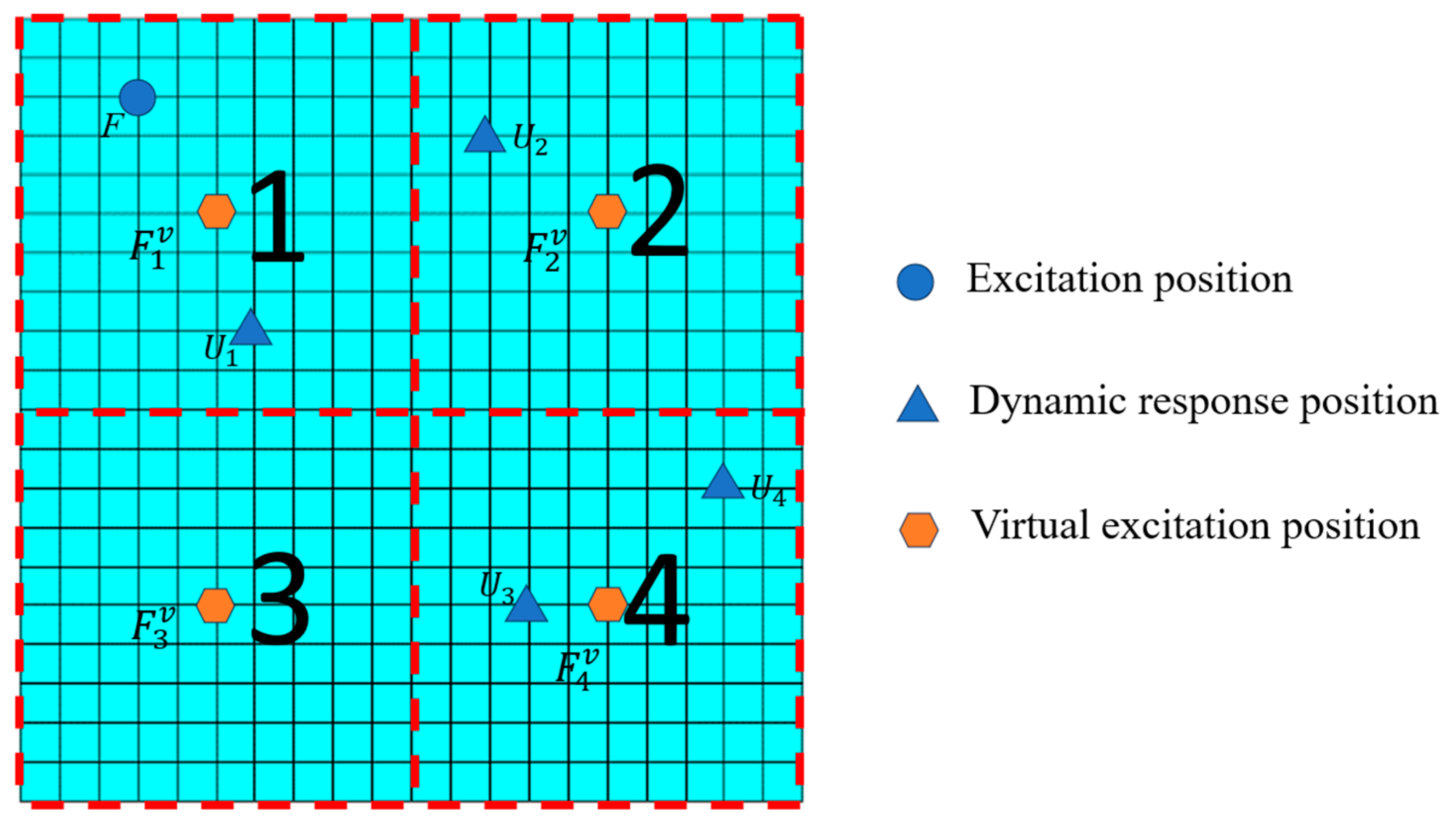
Since Equation (13) contains an unknown position quantity $(x,y)$, $\left[F\right]$ cannot be solved directly. Below, a case of the flat plate as an example to illustrate the method to identify the dynamic load step-by-step (the model is shown in Figure 1).

In Figure 1, the blue circle denotes the excitation position, the blue triangles are the dynamic response positions, and the yellow hexagons are the virtual excitation positions. In real-life applications, the exact location of the real dynamic load is unknown, so the response points are used to measure the dynamic response and calculate the correlation coefficients. To improve the calculation accuracy, the number of response points can be increased as is appropriate, and their positions can be randomly selected within the structure, provided that they are not overly concentrated in any particular area.

When the action position of the dynamic load is unknown, Equation (13) can be applied when using the general FRF method to represent the above dynamic load, with $\tilde{H}(x,y)$ being an unknown function, related to the coordinates of the dynamic load. The method proposed in this paper can avoid the unknown FRF relationship and can find the location of dynamic load by gradually reducing the range for the acceleration responses of known points.

So, the plate model is discretized into the FE mesh, and the domain is divided into four regions (numbered 1, 2, 3 and 4). Virtual excitation positions are selected in each region, as shown in Figure 1 $F_i^v$ ($i=1,2,3\mathrm{a}\mathrm{n}\mathrm{d}4$), and multiple dynamic response points are selected. Then, the dynamic response under virtual excitation is ${\ddot{u}}_{j,Vi}$ ($i=1,2,\dots ,k;j=1,2,\dots ,l$), where k is the number of virtual excitation points and l is the number of dynamic response points. Then, Equation (13) can be written as

$$\left[\begin{array}{cccc}{H}_{11}& H_{12}& \cdots & H_{1n}\\ H_{21}& H_{22}& \cdots & H_{2n}\\ ⋮& ⋮& \ddots & ⋮\\ H_{n1}& H_{n2}& \cdots & H_{nn}\end{array}\right]\left[\begin{array}{c}\begin{array}{c}0\\ ⋮\\ F_1^v\end{array}\\ 0\\ ⋮\\ \begin{array}{c}{F}_2^v\\ 0\\ ⋮\\ \begin{array}{c}{F}_k^v\\ 0\\ ⋮\\ 0\end{array}\end{array}\end{array}\right]=\left[\begin{array}{c}\begin{array}{c}0\\ ⋮\\ {\ddot{u}}_1^v\end{array}\\ 0\\ ⋮\\ \begin{array}{c}{\ddot{u}}_2^v\\ 0\\ ⋮\\ \begin{array}{c}{\ddot{u}}_l^v\\ 0\\ ⋮\\ 0\end{array}\end{array}\end{array}\right],$$

(14)

Equation (14) can be simplified as

$$\left[\begin{array}{ccc}{H}_{{\ddot{u}}_1{V}_1}& \cdots & H_{{\ddot{u}}_1{V}_k}\\ ⋮& \ddots & ⋮\\ H_{{\ddot{u}}_l{V}_1}& \cdots & H_{{\ddot{u}}_l{V}_k}\end{array}\right]\left[\begin{array}{c}{F}_1^v\\ ⋮\\ ⋮\\ F_k^v\end{array}\right]=\left[\begin{array}{c}{\ddot{u}}_1^v\\ ⋮\\ ⋮\\ {\ddot{u}}_l^v\end{array}\right],$$

(15)

In Equation (15), $H_{{\ddot{u}}_l{V}_k}$ is the acceleration FRF between the external excitation $F_k^v$ and the dynamic response ${\ddot{u}}_l^v$. Because the positions of the virtual excitation points and the positions of the acceleration response points are artificially selected, the acceleration FRF matrix can be changed from the previously unknown function related to the coordinates into a known matrix, and the order of this matrix can be further reduced. When both k and l are equal to 4, the FRF matrix in Equation (15) can be further simplified:

$$\left[\begin{array}{cccc}{H}_{11}& H_{12}& \cdots & H_{1n}\\ H_{21}& H_{22}& \cdots & H_{2n}\\ ⋮& ⋮& \ddots & ⋮\\ H_{n1}& H_{n2}& \cdots & H_{nn}\end{array}\right]\Rightarrow \left[\begin{array}{cccc}{H}_{11}& H_{12}& H_{13}& H_{14}\\ H_{21}& H_{22}& H_{23}& H_{24}\\ H_{31}& H_{32}& H_{33}& H_{34}\\ H_{41}& H_{42}& H_{43}& H_{44}\end{array}\right],$$

(16)

Thus, the dimension of the FRF matrix is further reduced. From Equation (12), the following relation can be obtained:

$$[{\ddot{u}}^v]=[H][F^v],$$

(17)

where $\left[F^v\right]$ is the virtual excitation force vector, $\left[H\right]$ is simplified FRF matrix. When the virtual excitation $\left[F^v\right]$ is applied at the virtual excitation point in the FE software (Patran), the acceleration response is $[{\ddot{u}}^v]$.

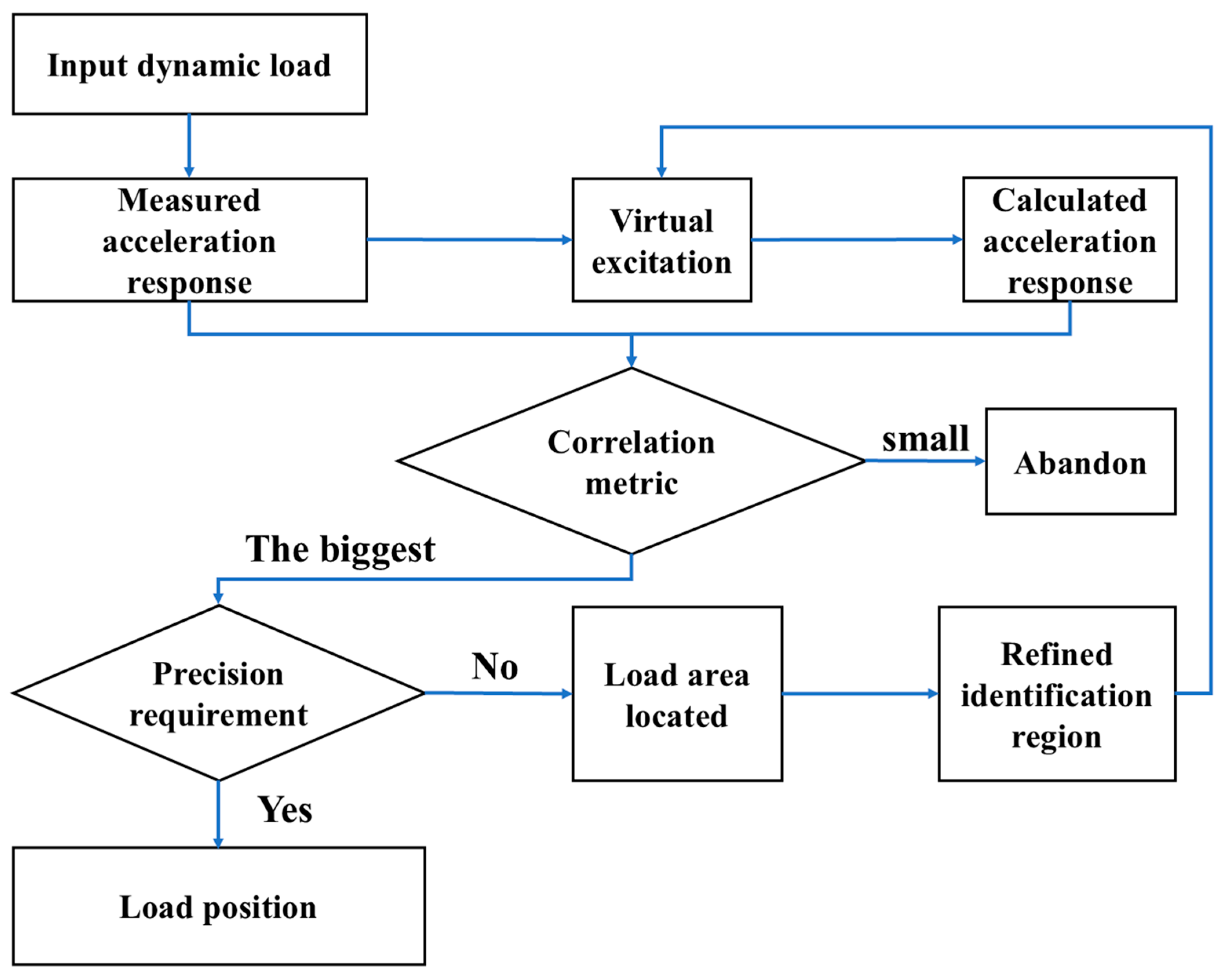
The acceleration responses $[\ddot{u}]$ obtained in experiments and the virtual acceleration responses $[{\ddot{u}}^v]$ obtained in simulations are used to calculate the correlation metrics in Equation (11). The area with the highest correlation metric contains the dynamic load. This process of subdivision within the defined region is repeated until the determined dynamic load position meets the desired accuracy. The center point of the recorded area is used as the dynamic load position.

2.4. Applicability and Limitations of the Method

2.4.1. Applicability of the Method

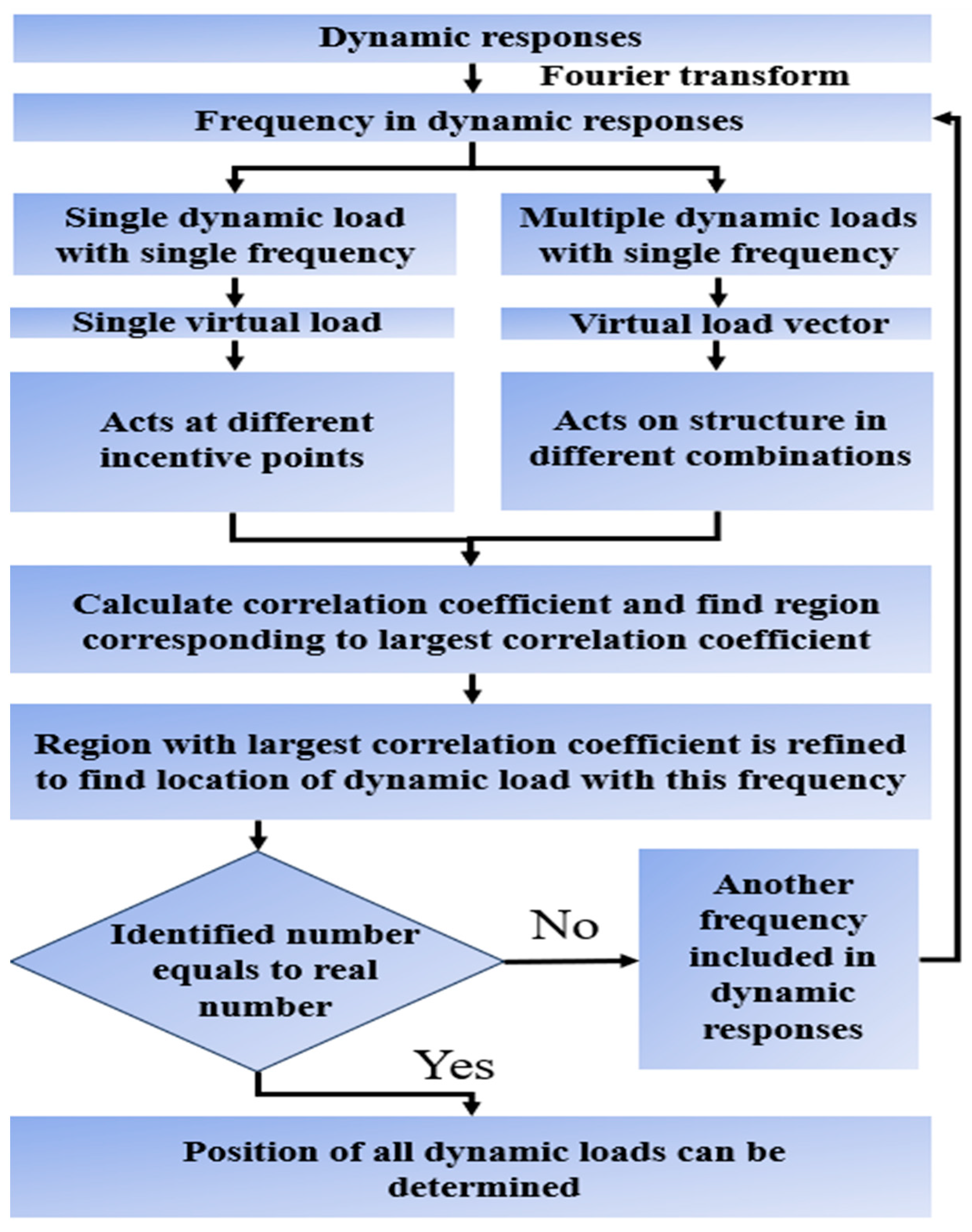
The method proposed in this paper can be applied not only to two-dimensional thin plates, but also extends to one-dimensional beam structures and three-dimensional structures. The main difference when applied to other engineering structures lies in the change in the FRF between the response and excitation points due to the number of position coordinate variables. For example, the FRF is $\mathrm{H}\left(\mathrm{x}\right)$ for one-dimensional structures, $\mathrm{H}(\mathrm{x},\mathrm{y})$ and $\mathrm{H}(\mathrm{x},\mathrm{y},\mathrm{z})$ for two-dimensional and three-dimensional structures, respectively. Additionally, when selecting virtual excitation points, they should be evenly distributed across the entire structure to obtain more comprehensive and accurate structural acceleration responses. As shown in Figure 2, the black circles represent the virtual load positions, and the black triangles represent the real load positions.

2.4.2. Limitations of the Method

The method proposed in this paper for dynamic load position identification has two main limitations: (1). When identifying more than one dynamic load, the loads cannot be too close to each other. (2). Before re-identifying the dynamic loads, the number of loads must be known in advance.

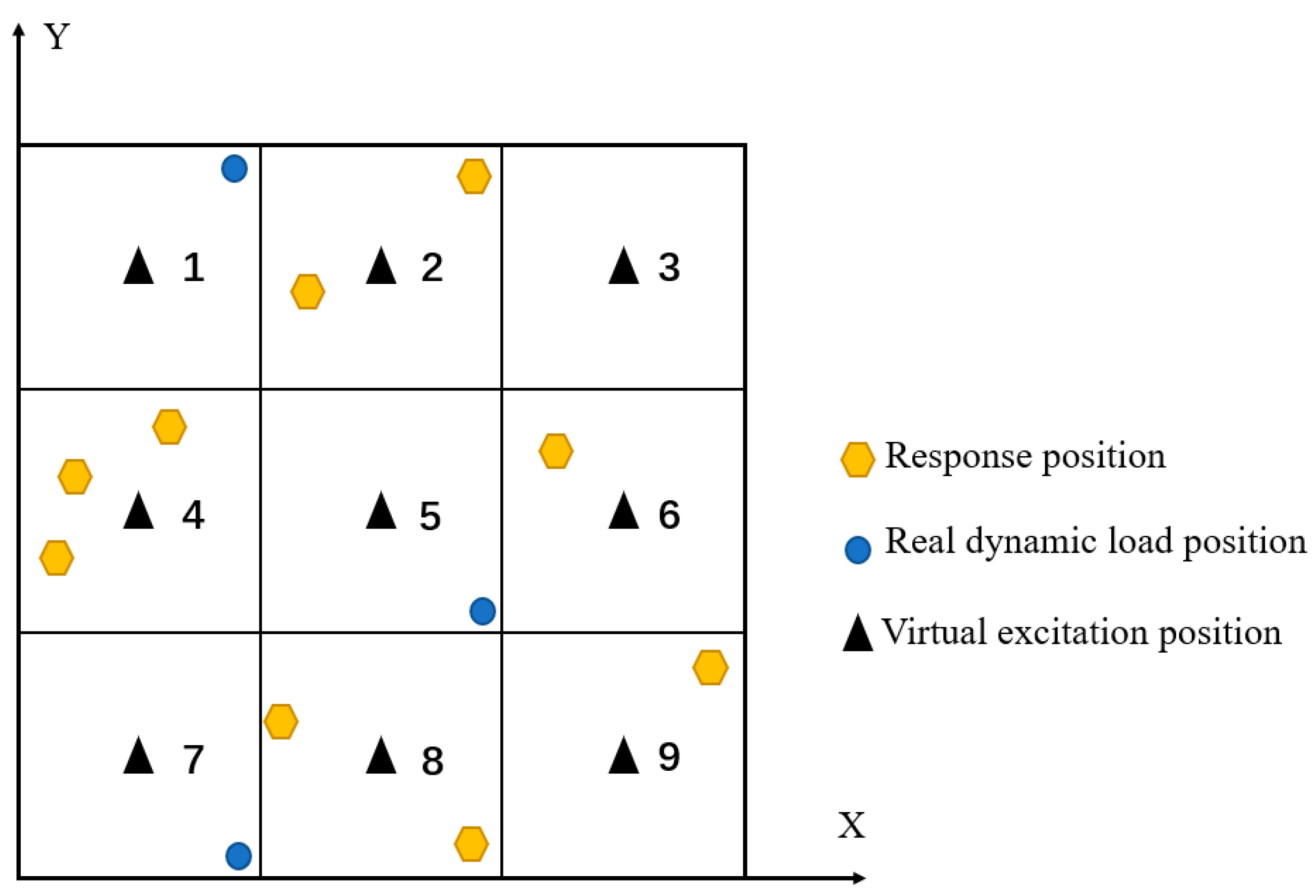
For limitation 1, consider the identification of the positions of two dynamic loads as an example. When these loads are too close to each other, the situation shown in Figure 3 may occur during the initial identification.

During the first identification, virtual loads are applied at four excitation points according to the original method, and the correlation metric M for their combinations is calculated. This results in six sets of data. By comparing these sets, the region with the highest correlation metric is retained. However, due to the positions of these two dynamic loads being too close within the same area, the first step of position identification incorrectly selects regions 1 and 2 as the locations of the dynamic loads. This leads to errors in the subsequent identification process. Therefore, a prerequisite for using the proposed method to identify multiple dynamic load positions is that the positions of the dynamic loads should not be too close to each other, as this will cause errors in the first step of identification.

For limitation 2, this represents a major challenge currently faced in the identification of dynamic load positions. Existing research on dynamic load position identification mostly focuses on the assumption of a known number of dynamic loads. This is because when multiple dynamic loads act on the same structure, the structural dynamic response is often complex, coupling information from multiple dynamic loads. Moreover, dynamic load position identification is a typical inverse problem, which can have non-unique solutions. If the number of loads is unknown at the input stage, this exacerbates the issue, leading to non-unique results and making it impossible to accurately determine the positions of the dynamic loads.

These two limitations are critical issues that need to be addressed in future dynamic load position identifications. In upcoming research, to relax these limitations, we will refer to methods proposed by other researchers for dynamic load position identification on composite materials. Prior to identifying the dynamic load positions, we will first use triangulation to determine the number of dynamic loads acting on the structure and the approximate distances between them. Triangulation leverages the mathematical relationship between the impact point, wave speed, and the time required for the shock wave to reach different measurement points, representing the dynamic load position identification problem as the geometric relationship between the sensors and the shock waves. Since dynamic loads at different locations on the structure generate shock waves of varying magnitudes, and the time for these waves to reach the detectors differs, the number of vibration responses collected by the detectors can be used to determine the number of dynamic loads. When multiple dynamic loads are detected, the time intervals between the responses collected by the sensors can be used to assess whether the dynamic loads are too close, thus guiding the next steps of the operation.

3. Virtual Excitation Load

As demonstrated above, the identification process in this paper primarily involves the application of virtual loads at various excitation points to determine the correlation coefficients between the response under virtual excitation and the actual response. This helps to narrow down the region of interest, followed by the subsequent application of virtual excitation within this reduced region to approximate the real load position. This section deals with determining the virtual loads under different external dynamic conditions.

3.1. Single-Point Dynamic Load with One Frequency

When the input dynamic load is a single-point with only one frequency, the identification process is relatively simple since for this the input load is presented in the following form:

$$F=A_1\sin (\omega t+\theta ),$$

(18)

the response of the system at multiple points can be described as

$$\left\{\begin{array}{c}{\ddot{u}}_1=\left|H_1\right|A\sin (\omega t+\theta +\varphi (H_1))\\ ⋮\\ {\ddot{u}}_m=\left|H_m\right|A\sin (\omega t+\theta +\varphi (H_m))\end{array}\right.,$$

(19)

Which also has only this one frequency. Thus, the frequency of the desired virtual excitation can be obtained with the Fourier transform of the acceleration responses, and the virtual excitation $F^v=\sin \left(\omega t\right)$ can be obtained.

3.2. Single-Point Dynamic Load with Multiple Frequencies

For a single-point dynamic load with multiple frequency segments, its position can be identified only utilizing one of the frequencies. The specific identification steps are as follows. The dynamic load with multiple frequencies at the excitation point can be presented as

$$F=A_1\sin ({\omega }_{1}t+{\theta }_1)+A_2\sin ({\omega }_{2}t+{\theta }_2)+\cdots +A_n\sin ({\omega }_{n}t+{\theta }_n),$$

(20)

Here the frequencies are assumed to be ${\omega }_1<{\omega }_2<\cdots <{\omega }_n$. Then, the responses at the response points of the structure under the above dynamic load are as follows:

$$\left\{\begin{array}{c}{\ddot{u}}_1=\left|H_{11}\right|A_1\sin ({\omega }_{1}t+{\theta }_1+\varphi (H_{11}))+\cdots +\left|H_{1n}\right|A_n\sin ({\omega }_{n}t+{\theta }_n+\varphi (H_{1n}))\\ {\ddot{u}}_2=\left|H_{21}\right|A_1\sin ({\omega }_{1}t+{\theta }_1+\varphi (H_{21}))+\cdots +\left|H_{2n}\right|A_n\sin ({\omega }_{n}t+{\theta }_n+\varphi (H_{2n}))\\ ⋮\\ {\ddot{u}}_m=\left|H_{m1}\right|A_1\sin ({\omega }_{1}t+{\theta }_1+\varphi (H_{m1}))+\cdots +\left|H_{mn}\right|A_n\sin ({\omega }_{n}t+{\theta }_n+\varphi (H_{mn}))\end{array}\right.,$$

(21)

where $\left|H_{ij}\right|$ and $\varnothing \left(H_{ij}\right)\left(1\le i\le m,1\le j\le n\right)$ are the amplitude and the phase of the FRF between the real dynamic load and the ith response point at the frequency ${\omega }_j$, respectively.

It is evident from Equation (21) that these m dynamic responses are all linearly superposed by fragments at n different frequencies, with these n frequencies encompassed in the dynamic load in Equation (20). Hence, the Fourier transform can be performed on Equation (21) to acquire all the frequencies involved in the actual dynamic load. Then, the frequency value $\mathsf{\omega }=\left[{\omega }_1{ \omega }_2\cdots {\omega }_n\right]$ can be obtained for this dynamic load. Using one of these frequencies (taking ${\omega }_1$ as an example), the unit virtual load $F^v=\sin \left({\omega }_{1}t\right)$ is constructed, while all dynamic responses with frequency ${\omega }_1$ are selected from the m response points in Equation (21). The virtual unit load with frequency ${\omega }_1$ is applied to different excitation points, and the correlation metric between the response under virtual excitation and the dynamic response with the same frequency in Equation (21) is calculated. The region corresponding to the excitation point with the largest correlation metric is then selected and divided into the sub-regions again. The above steps are repeated to find the location of the dynamic load.

3.3. Multi-Point Dynamic Loads with Single Frequency

There is a precondition that the number of dynamic loads is known in the process of identification of the position of multi-point dynamic loads in this paper.

For multiple dynamic loads with the same frequency, the method to determine virtual loads $\left[F^v\right]$ is similar to the one above, and the main steps are as follows:

$$[F]=\left[\begin{array}{c}{A}_1\sin (\omega t+{\theta }_1)\\ A_2\sin (\omega t+{\theta }_2)\\ ⋮\\ A_n\sin (\omega t+{\theta }_n)\end{array}\right],$$

(22)

$$\left\{\begin{array}{c}{\ddot{u}}_1=\left|H_{11}\right|A_1\sin (\omega t+{\theta }_1+\varphi (H_{11}))+\cdots +\left|H_{1n}\right|A_n\sin (\omega t+{\theta }_n+\varphi (H_{1n}))\\ {\ddot{u}}_2=\left|H_{21}\right|A_1\sin (\omega t+{\theta }_1+\varphi (H_{21}))+\cdots +\left|H_{2n}\right|A_n\sin (\omega t+{\theta }_n+\varphi (H_{2n}))\\ ⋮\\ {\ddot{u}}_m=\left|H_{m1}\right|A_1\sin (\omega t+{\theta }_1+\varphi (H_{m1}))+\cdots +\left|H_{mn}\right|A_n\sin (\omega t+{\theta }_n+\varphi (H_{mn}))\end{array}\right.,$$

(23)

Equation (22) represents the input dynamic load vector, and Equation (23) is the acceleration responses at the response points on the structure under these dynamic loads. It is evident from Equation (23) that these responses are formed by superposition of a series of sinusoidal signals with frequency $\mathsf{\omega }$. Therefore, the measured acceleration responses can be Fourier transformed to obtain the frequency of these dynamic loads and thus the virtual load vector $\left[F^v\right]$ that should be applied:

$$[F^v]=\left[\begin{array}{c}\sin (\omega t)\\ \sin (\omega t)\\ ⋮\\ \sin (\omega t)\end{array}\right],$$

(24)

3.4. Multi-Point Dynamic Loads with Multiple Frequencies

When the case to be identified deals with multiple dynamic loads with multiple different frequencies, it is first assumed that all input dynamic loads have a specific frequency $\mathsf{\omega }$. In this case, the construction of virtual loads can be simplified to the above method of multiple dynamic loads with a single frequency. At this time, the frequency of the virtual load can be obtained after the Fourier transform of the dynamic responses, and then the virtual load in Equation (24) can be constructed according to the number of dynamic loads.

When it cannot be determined in advance whether all dynamic loads have a particular frequency, two distinct recognition processes emerge. In the first scenario, the initially identified frequency is present simultaneously in several different dynamic loads, while in the second scenario, the frequency is present only in one dynamic load. In these cases, the virtual load should be combined in different ways and, subsequently, the maximum correlation metric is utilized to determine the number of regions where this frequency is active. In the first scenario, when the initially identified frequency exists across multiple regions simultaneously, the locations of multiple dynamic loads at this frequency can be progressively refined in the identified regions. Once the identification of the first frequency’s load location is completed, if the number of identified dynamic loads matches the actual number of dynamic loads, the identification process concludes. If the number is fewer than the actual number of dynamic loads, the next frequency is selected, and the above steps are repeated to accomplish the identification. In the second scenario, the identified region can be subdivided to pinpoint the location of a dynamic load. Subsequently, the next frequency can be identified, and the aforementioned steps are iterated until the number of identified dynamic loads matches the input. This identification process is exemplified by an instance where there are two dynamic loads with four response points and virtual excitation points:

$$\left\{\begin{array}{c}{F}_1=A_1\sin ({\omega }_{1}t+{\theta }_1)+A_2\sin ({\omega }_{2}t+{\theta }_2)+\cdots +A_n\sin ({\omega }_{n}t+{\theta }_n)\\ F_2={\overline{A}}_1\sin ({\overline{\omega }}_{1}t+{\overline{\theta }}_1)+{\overline{A}}_2\sin ({\overline{\omega }}_{2}t+{\overline{\theta }}_2)+\cdots +{\overline{A}}_n\sin ({\overline{\omega }}_{n}t+{\overline{\theta }}_n)\end{array}\right.,$$

(25)

Equation (25) shows that there are two real input dynamic loads with multiple frequencies. When the two dynamic loads act on the structure, the dynamic responses of the structure are as follows:

$$\left\{\begin{array}{c}\begin{array}{l}{\ddot{u}}_1=\left|H_{11}\right|A_1\sin ({\omega }_{1}t+{\theta }_1+\varphi (H_{11}))+\cdots +\left|H_{1n}\right|A_n\sin ({\omega }_{n}t+{\theta }_n+\varphi (H_{1n}))\\ +\left|H_{1(n+1)}\right|{\overline{A}}_1\sin ({\overline{\omega }}_{1}t+{\overline{\theta }}_1+\varphi (H_{1(n+1)}))+\cdots +\left|H_{1(2n)}\right|{\overline{A}}_n\sin ({\overline{\omega }}_{n}t+{\overline{\theta }}_n+\varphi (H_{1(2n)}))\end{array}\\ \begin{array}{l}{\ddot{u}}_2=\left|H_{21}\right|A_1\sin ({\omega }_{1}t+{\theta }_1+\varphi (H_{21}))+\cdots +\left|H_{2n}\right|A_n\sin ({\omega }_{n}t+{\theta }_n+\varphi (H_{2n}))\\ +\left|H_{2(n+1)}\right|{\overline{A}}_1\sin ({\overline{\omega }}_{1}t+{\overline{\theta }}_1+\varphi (H_{2(n+1)}))+\cdots +\left|H_{2(2n)}\right|{\overline{A}}_n\sin ({\overline{\omega }}_{n}t+{\overline{\theta }}_n+\varphi (H_{2(2n)}))\end{array}\\ ⋮\\ \begin{array}{l}{\ddot{u}}_4=\left|H_{41}\right|A_1\sin ({\omega }_{1}t+{\theta }_1+\varphi (H_{41}))+\cdots +\left|H_{4n}\right|A_n\sin ({\omega }_{n}t+{\theta }_n+\varphi (H_{4n}))\\ +\left|H_{4(n+1)}\right|{\overline{A}}_1\sin ({\overline{\omega }}_{1}t+{\overline{\theta }}_1+\varphi (H_{4(n+1)}))+\cdots +\left|H_{4(2n)}\right|{\overline{A}}_n\sin ({\overline{\omega }}_{n}t+{\overline{\theta }}_n+\varphi (H_{4(2n)}))\end{array}\end{array}\right.,$$

(26)

After the acceleration responses at the four points in Equation (26) are obtained, the Fourier transform is performed on them to obtain all frequencies $[\omega ]=[\begin{array}{cccc}\begin{array}{ccc}{\omega }_1& \cdots & {\omega }_n\end{array}& {\overline{\omega }}_1& \cdots & {\overline{\omega }}_n\end{array}]$ for the two dynamic loads. One frequency ${\omega }_c$ ($1\le \mathrm{c}<n$) is selected as an example to establish virtual excitation $F^v=\sin \left({\omega }_{c}t\right)$ (Usually starting with the smallest frequency, which is ${\omega }_c={\omega }_1$). At this time, because it is not known whether the frequency is present in one dynamic load or two dynamic loads, the first step is to assume that the frequency is only in one dynamic load. Then, the established virtual load is applied to the four excitation points in turn, and the correlation coefficients between the responses under virtual excitation and the part with the same frequency in the actual dynamic responses are calculated.

After finding four correlation metrics for the above part, and assuming that two dynamic loads have this frequency, which means ${\omega }_c={\overline{\omega }}_c$, the next step is to select two of the four regions and apply the virtual loads on the excitation points; this should be carried out six times in total. The virtual load for this step should be as follows:

$$[F^v]=\left[\begin{array}{c}\sin ({\omega }_{c}t)\\ \sin ({\omega }_{c}t)\end{array}\right],$$

(27)

Comparing all the above correlation metrics to select the maximum value. If the virtual excitation corresponding to this value is applied to only one region, then the location of one of the dynamic loads can be obtained by continuously refining this region. Subsequently, the next frequency ${\omega }_{c+1}$ is selected to establish the virtual excitation $F^v=\sin \left({\omega }_{c+1}t\right)$ and the aforementioned steps are repeated for identification. If the virtual excitation corresponding to this value is applied to two different regions, then two dynamic loads have this frequency and these two regions are the locations of two dynamic loads. Through continuous refinement based on the virtual excitation at this frequency, the locations of the two dynamic loads can be identified. This identification problem thereby converts into the aforementioned problem for multiple dynamic load points with the same frequency, discussed above.

From the mentioned construction of the virtual unit load, it is evident that the creation of the virtual load primarily depends on the Fourier transform of the structure’s acceleration responses. There are two possible scenarios for the acceleration response obtained through the Fourier transform: (i) The response has only a single frequency, and (ii) the response has multiple frequencies. In the former case, if there is only one dynamic load, the virtual load $F^v=\sin \left(\omega t\right)$ can be directly established based on the response frequency. If there are multiple dynamic loads, the virtual load can be constructed according to Equation (24), which accounts for the number of dynamic loads. For responses with multiple frequencies, if there is only one dynamic load, this indicates that this load has multiple different frequencies simultaneously. To identify the location of the dynamic load, one of these frequencies should be selected and the virtual load $F^v=\sin \left({\omega }_{1}t\right)$ should be established. By calculating the correlation coefficient between the responses under this virtual load and the actual acceleration responses with this frequency, the position of the real load can be progressively approximated. When the acceleration responses have multiple frequencies and there are multiple dynamic loads, the procedure begins with the selection of one frequency to establish the virtual load. The number of dynamic loads with this frequency is then calculated using the correlation coefficient. If multiple dynamic loads share this frequency, the problem transforms into the construction of a virtual excitation for the above case of multiple dynamic loads with the same frequency. If only one dynamic load has this frequency, the construction follows the same methodology as for a single dynamic load. After identifying the position of the dynamic load associated with this frequency, if the total number of dynamic loads exceeds the identified ones, the aforementioned steps are repeated until all dynamic loads are determined. A flow chart for the location identification of multiple dynamic loads with multiple frequencies is given in Figure 4.

As can be seen from the above construction method of virtual dynamic loads, the problem of location identification for dynamic loads with multiple frequencies can be transformed into those for multi-point dynamic loads with a single frequency and a single-point dynamic load with one frequency by the Fourier transform. Thus, a thin plate is taken as an example to illustrate the steps necessary to identify the locations of multiple dynamic loads with the same frequency:

• In this example, there are three dynamic loads, and the number of virtual excitation points and response points is 9. It is assumed that the frequency of all dynamic loads is ω. The schematic diagram of this example is given in Figure 5, where the blue circles are the positions of real dynamic load, the black triangles are the positions of virtual excitation, and the yellow hexagons are the positions of response.
• First, the response data of the response points are collected after the action of dynamic loads. According to Equations (22) and (23), these acceleration responses are Fourier transformed to obtain their forms in the frequency domain to obtain the virtual excitation. Virtual load in Figure 5 is ${\left[F^v\right]}^T=\left[\mathrm{s}\mathrm{i}\mathrm{n}\left(\omega t\right)\mathrm{s}\mathrm{i}\mathrm{n}\left(\omega t\right)\mathrm{s}\mathrm{i}\mathrm{n}\left(\omega t\right)\right]$.
• The second step is to select the first three regions out of nine and apply the unit virtual loads to them at the same time. The positions of the loads are in the center of each region, so that ${\left[F^v\right]}^T=\left[\begin{array}{ccc}{F}_1^v& F_2^v& F_3^v\end{array}\right]=\left[\begin{array}{ccc}\mathrm{s}\mathrm{i}\mathrm{n}\left(\omega t\right)& \mathrm{s}\mathrm{i}\mathrm{n}\left(\omega t\right)& \mathrm{s}\mathrm{i}\mathrm{n}\left(\omega t\right)\end{array}\right]$$F_n^v$ indicates the virtual load applied on the nth region).
• The responses ${\left[{\ddot{u}}^v\right]}^T=\left[{\ddot{u}}_1^v {\ddot{u}}_2^v \cdots {\ddot{u}}_9^v\right]$ at nine acceleration response points are measured, and the average correlation metric ${\overline{M}}_1$ between the obtained virtual response $\left[{\ddot{u}}^v\right]$ and the measured real response is calculated.
• Change the area of the virtual unit load in step 3, so that ${\left[F^v\right]}^T=\left[\begin{array}{ccc}{F}_1^v& F_2^v& F_4^v\end{array}\right]=\left[\begin{array}{ccc}\mathrm{s}\mathrm{i}\mathrm{n}\left(\omega t\right)& \mathrm{s}\mathrm{i}\mathrm{n}\left(\omega t\right)& \mathrm{s}\mathrm{i}\mathrm{n}\left(\omega t\right)\end{array}\right]$, and repeat step 4 to calculate correlation metric.
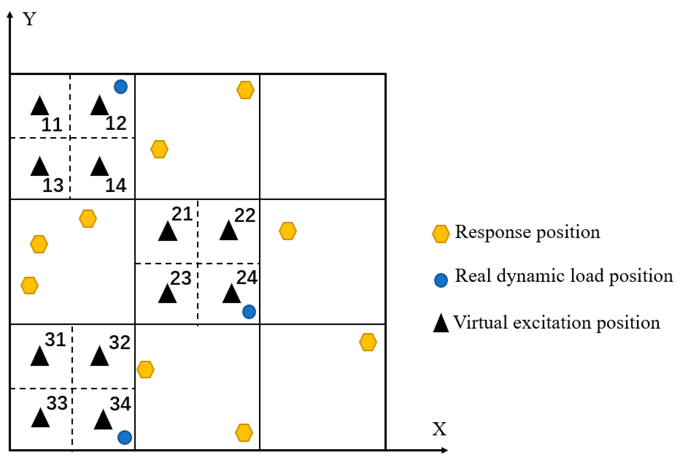
• Comparing ${\overline{M}}_1,{\overline{M}}_2$ ……${\overline{M}}_{\delta }$, find three regions corresponding to the largest $\overline{M}$, divide each region into four sub-regions (Figure 6), and number each region (for example, n1 represents block 1 in the nth region). In Figure 6, black triangles are the new virtual load positions in the second identification process.
• After the completion of the above steps, the first stage of dynamic load identification is completed. Select a small sub-region from each of the three regions to jointly apply the unit virtual load. Let ${\left[F^v\right]}^T=\left[\begin{array}{ccc}{F}_{11}^v& F_{21}^v& F_{31}^v\end{array}\right]=\left[\begin{array}{ccc}\mathrm{s}\mathrm{i}\mathrm{n}\left(\omega t\right)& \mathrm{s}\mathrm{i}\mathrm{n}\left(\omega t\right)& \mathrm{s}\mathrm{i}\mathrm{n}\left(\omega t\right)\end{array}\right]$ and calculate the new response ${\left[{\ddot{u}}^v\right]}^T=\left[{\ddot{u}}_1^v {\ddot{u}}_2^v \cdots {\ddot{u}}_9^v\right]$ and the influence metric ${\check{M}}_1$($F_{mn}^v$ indicates that the unit virtual load is applied to the sub-region nth in the region m).
• Change the virtual load applied in the region in step 7, that is, ${\left[F^v\right]}^T=\left[\begin{array}{ccc}{F}_{11}^v& F_{21}^v& F_{32}^v\end{array}\right]=\left[\begin{array}{ccc}\mathrm{s}\mathrm{i}\mathrm{n}\left(\omega t\right)& \mathrm{s}\mathrm{i}\mathrm{n}\left(\omega t\right)& \mathrm{s}\mathrm{i}\mathrm{n}\left(\omega t\right)\end{array}\right]$. Calculate $\left[{\ddot{u}}^v\right]$ and ${\check{M}}_2$.
• Repeat step 8 until ${\check{M}}_c$ are calculated. At this stage, the virtual load (Figure 3) is ${\left[F^v\right]}^T=\left[\begin{array}{ccc}{F}_{14}^v& F_{24}^v& F_{34}^v\end{array}\right]=\left[\begin{array}{ccc}\mathrm{s}\mathrm{i}\mathrm{n}\left(\omega t\right)& \mathrm{s}\mathrm{i}\mathrm{n}\left(\omega t\right)& \mathrm{s}\mathrm{i}\mathrm{n}\left(\omega t\right)\end{array}\right]$(where C = $4^3=64$).
• Find three sub-regions corresponding to the maximum value ${\check{M}}_{max}$ in ${\check{M}}_1,{\check{M}}_2$……${\check{M}}_c$, and then repeat steps 6–8 until the grids’ size for the recognition areas is small. For a very fine mesh, the recognition process can become cumbersome, so the process should be stopped. Then, the region identified in the last step can be considered as the location of the real dynamic load.

The above steps describe the process of identification of the positions of multiple dynamic loads with a single frequency. When the dynamic loads have multiple different frequencies, it is necessary to obtain the frequency distribution of the acceleration responses with the Fourier transformation. Subsequently, the correlation metrics are computed between the acceleration responses of the structure following the application of a virtual load at a specific frequency and the responses at this frequency in the actual acceleration data. Once the position of a dynamic load with specific frequency is obtained, proceed to calculate for subsequent frequencies using the methods outlined in the preceding steps.

The specific steps of using stepwise identification for dynamic loads are shown in Figure 7.

4. Simulation Example

Simulation verification is conducted based on the step-by-step identification method outlined above. A four-sided simply supported thin plate is utilized, with its parameters listed in

Table 1. Structural parameters of thin plate.

Parameter	Length/m	Width/m	Thickness/m	Elastic Modulus/GPa	Poisson’s Coefficient	Density/kg/m3	Damping Ration
Parameter value	1	1	0.01	70	0.3	2700	0.03

.

In practical engineering applications, measurement noise and the number of sensors are two key factors that influence the results of dynamic load identification. Therefore, in this chapter, we will conduct identifications of dynamic responses under three conditions: no noise, 5% noise, and 10% noise. Additionally, two different operational conditions will be set: (1) four accelerometer sensors on the thin plate, and (2) nine accelerometer sensors on the thin plate. The positions of the sensors under these different conditions are shown in Figure 8, where the black triangles represent the accelerometer sensors.

4.1. Single-Point Excitation

4.1.1. Noise-Free Identification of Single-Point Dynamic Load Under Operational Condition 1

In Figure 9, the blue triangles denote the response positions, black hexagons denote the virtual excitation positions, while the blue circle shows the true excitation position.

Specific location information is provided in

Table 2. Locations of excitation position and response position.

	Excitation Position 1/m	Response Position 1/m	Response Position 2/m	Response Position 3/m	Response Position 4/m
x	0.2	0.25	0.75	0.25	0.75
y	0.8	0.75	0.75	0.25	0.25

.

A single-point harmonic excitation $f\left(t\right)=10\sin \left(20\pi t\right)$ is applied to the thin plate, with the excitation position corresponding to the location of the circular point in Figure 6. Four acceleration responses are then obtained, with the response point positions indicated by the triangular symbol in Figure 9. After the Fourier transformation of the acceleration responses at four response points, the frequency $\mathsf{\omega }=20\mathsf{\pi }$ of the input dynamic load can be obtained, from which the virtual unit load $F^v\left(t\right)=\sin \left(20\pi t\right)$ can be established.

In the initial step of identification, a virtual excitation position is selected on the thin plate, as illustrated in Figure 9. A unit excitation is then applied to this virtual position using finite-element software, resulting in virtual acceleration. Subsequently, the correlation metrics between the virtual acceleration responses and the actual ones are calculated by solving Equation (11). The specific locations where the virtual loads are applied in each identification step are shown in

Table 3. Virtual excitation locations.

	Step 1				Step 2				Step 3
	1	2	3	4	1	2	3	4	1	2	3	4
x	0.25	0.75	0.25	0.75	0.125	0.375	0.125	0.375	0.0625	0.1875	0.0625	0.1875
y	0.75	0.75	0.25	0.25	0.875	0.875	0.625	0.625	0.9375	0.9375	0.8125	0.8125

.

The described method is iterated until either the difference in correlation metrics becomes small or the size of sub-regions in the region decreases. The correlation metrics obtained from the step-by-step identification process are presented in

Table 4. Correlation metrics of noise-free single-point recognition under Operational condition 1.

	Step 1				Step 2				Step 3
Location number	1	2	3	4	1	2	3	4	1	2	3	4
Correlation metric	6.47	4.33	4.33	4.07	6.16	5.44	5.44	5.21	5.73	5.84	5.84	7.84

.

As observed in Table 4, the first correlation metrics are the highest in the first and the second identification steps, while the fourth correlation metric for the third identification step is the highest. Consequently, the identified excitation position progressively approaches the true value.

4.1.2. Identification Results of Single-Point Dynamic Load with Noise Under Operational Condition 1

The magnitude and position of the external excitation are consistent with those described earlier. The acceleration response data is collected from the four accelerometer sensors. Subsequently, 5% gaussian white noise is added to the collected acceleration response. Fourier transform can be used to obtain the main frequency of the external dynamic load that causes the vibration, from which the virtual unit load can be established. A unit excitation is then applied to virtual position using finite-element software, resulting in virtual acceleration. Subsequently, the correlation metric between the virtual acceleration responses and the actual ones with noise are calculated by solving Equation (11). The Correlation metrics obtained from the step-by-step identification process are presented in

Table 5. Correlation metrics of single-point recognition with 5% noise under Operational Condition 1.

	Step 1				Step 2				Step 3
Location number	1	2	3	4	1	2	3	4	1	2	3	4
Correlation metric	3.0901	3.0645	3.0633	3.0419	3.0903	3.0883	3.0878	3.0858	3.0897	3.0901	3.0898	3.0905

.

As observed in Table 5, the first correlation metrics are the highest in the first and the second identification steps, while the fourth correlation metric for the third identification step is the highest. Consequently, the identified excitation position progressively approaches the true value. This indicates that even with 5% noise in the dynamic responses, the position of the single-point dynamic load on the thin plate can be accurately identified using the method proposed in this paper, provided there are four sensors in the structure.

By adding 10% Gaussian white noise to the obtained acceleration response and applying a unit virtual load at the selected virtual excitation points on the thin plate, the correlation metrics M can be calculated using the virtual acceleration responses at four points and the acceleration response data with 10% Gaussian white noise, resulting in

Table 6. Correlation metrics of single-point recognition with 10% noise under Operational Condition 1.

	Step 1				Step 2				Step 3
Location number	1	2	3	4	1	2	3	4	1	2	3	4
Correlation metric	2.7539	2.7444	2.7420	2.7345	2.7536	2.7535	2.7526	2.7526	2.7533	2.7537	2.7532	2.7539

:

The first correlation metrics are the highest in the first and the second identification steps, while the fourth correlation metric for the third identification step is the highest. The above table indicates that even with 10% noise in the dynamic responses, the position of the single-point dynamic load on the thin plate can be accurately identified using the method proposed in this paper, provided there are four sensors in the structure.

4.1.3. Identification Results of Single-Point Dynamic Load with Noise Under Operational Condition 2

Under operating condition 2, there are nine acceleration response points in the structure, as show in Figure 8. The specific location information of response points under operating condition 2 is shown in

Table 7. Locations of nine response positions.

Response Number	1	2	3	4	5	6	7	8	9
x/m	0.25	0.5	0.75	0.25	0.5	0.75	0.25	0.5	0.75
y/m	0.75	0.75	0.75	0.5	0.5	0.5	0.25	0.25	0.25

.

By constructing a unit virtual load as described above and applying it to the selected excitation points, collecting the virtual acceleration responses at these points along with the acceleration data containing 5% Gaussian white noise to calculate the correlation metric M, the following identification data can be obtained, as shown in

Table 8. Correlation metrics of single-point recognition with 5% noise under Operational Condition 2.

	Step 1				Step 2				Step 3
Location number	1	2	3	4	1	2	3	4	1	2	3	4
Correlation metric	3.1025	3.0877	3.0796	3.0684	3.1027	3.1012	3.1012	3.0998	3.1024	3.1023	3.1028	3.1029

.

The first correlation metrics are the highest in the first and the second identification steps, while the fourth correlation metric for the third identification step is the highest. The above table shows that when the dynamic responses in working condition 2 contain 5% noise, the identification result of a single-point dynamic load is consistent with the previous text, and the overall identified correlation metrics are higher than that in operating condition 1.

Subsequently, 10% noise was added to the measured dynamic response, and the above steps were repeated to obtain the recognition result as shown in

Table 9. Correlation metrics of single-point recognition with 10% noise under Operational Condition 2.

	Step 1				Step 2				Step 3
Location number	1	2	3	4	1	2	3	4	1	2	3	4
Correlation metric	2.7577	2.7518	2.7469	2.7430	2.7576	2.7572	2.7568	2.7566	2.7573	2.7574	2.7574	2.7577

.

The first correlation metrics are the highest in the first and the second identification steps, while the fourth correlation metric for the third identification step is the highest. The above simulation shows that when there are nine acceleration response points and the response data contain 5% and 10% Gaussian white noise, the method proposed in this paper can identify the position of the single-point dynamic load on the thin plate. Moreover, compared to using only four acceleration response points, the correlation metrics calculated with nine response points is higher. This is because multiple acceleration response points provide a better representation of the overall vibration response on the thin plate, leading to more accurate results.

4.1.4. Identification Results of Single-Point Dynamic Load

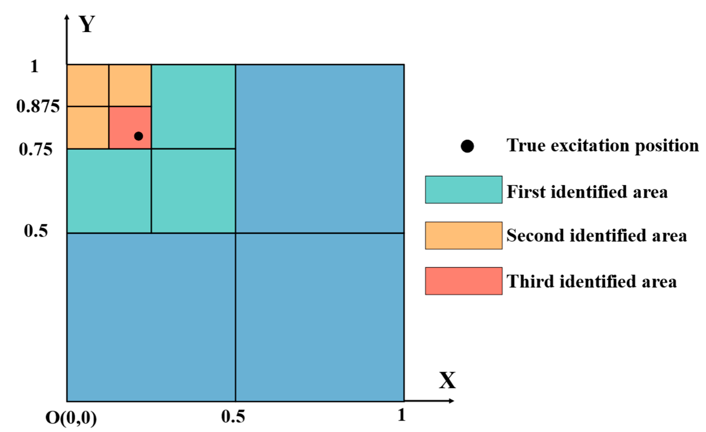
The specific identification process is depicted in Figure 10, and the results are shown in

Table 10. Results of step-by-step identification.

	Excitation Position/m
	x	y
True value	0.2	0.8
Identification result	0.1875	0.8125

.

4.1.5. Identification Accuracy

In this paper, since the structure used in the simulation experiment is a square thin plate, the calculation formula to define the experimental error rate has the following form.

$${\eta }_{error}={\displaystyle \frac{\frac{\left|x_t-x_i\right|}{L}+\frac{\left|y_t-y_i\right|}{W}}{2}}\times 100\%,$$

(28)

In Equation (28), $x_t$ is the real x-coordinate of the dynamic load, $x_i$ is the x-coordinate of the dynamic load identified using the proposed method, $y_t$ is the real y-coordinate of the dynamic load, and $y_i$ is the y-coordinate of the dynamic load identified using the proposed method. L and W are the length and the width of the structure, respectively. In the simulation experiment, the two values are 1 m for the square thin plate. The position error of the step-by-step recognition is 1.25%, indicating high recognition accuracy.

4.1.6. Computational Time for the Identification of Single Point Dynamic Load

After a demonstration of the feasibility of recognition, the computational requirements of this method are compared with those of the general method. Initially, the thin plate is divided into regions, as shown in Figure 1. This division results in a total of 400 elements and 441 nodes. Under operational condition 1, in the first measurement step, the virtual loads are applied to four virtual excitation points, and four response data points are measured. This requires the total of 16 dynamic response data to be measured. Subsequently, at each sub-step, four virtual excitations are applied, and 16 dynamic responses are measured. Across 3 steps, 12 virtual excitations are required to measure 48 dynamic responses. In comparison, the general method would necessitate 441 virtual loads and 1764 dynamic response measurements. Under operational condition 2, in the first measurement step, the virtual loads are applied to four virtual excitation points, and nine response data points are measured. This requires the total of 36 dynamic response data to be measured. Subsequently, at each sub-step, 4virtual excitations are applied, and 36 dynamic responses are measured. Across 3 steps, 12 virtual excitations are required to measure 108 dynamic responses. In comparison, under operational condition 1, the general method would necessitate 441 virtual loads and 1764 dynamic response measurements. Under operational condition 2, the general method would necessitate 441 virtual loads and 3969 dynamic response measurements.

Therefore, this method apparently significantly reduces the calculation time and increases solving efficiency compared to the general dynamic load identification method.

Table 11. Comparison of computation for identification of single-point dynamic load between traditional and step-by-step methods.

	Number of Applied Loads	Number of Response Data	Number of Loads Applied in Traditional Method	Number of Responses Collected in Traditional Method
Step 1	4	16/36	441	1764/3969
Step 2	8	32/72
Step 3	12	48/108

shows the number of virtual loads that should be applied and the number of measured responses in the traditional method and the method used in this paper.

4.2. Multi-Point Excitation

It can be seen from the single-point excitation in Section 4.1 that the stepwise identification method is feasible. This section continues to verify the feasibility of the stepwise identification method for the multi-point excitations.

4.2.1. Noise-Free Identification of Multi-Point Dynamic Loads Under Operational Condition 1

Two excitations $f_1$ and $f_2$ are applied on the sheet.

$$\left\{\begin{array}{c}{f}_1(t)=10\sin (40\pi t)\\ f_2(t)=20\sin (40\pi t)\end{array}\right.,$$

(29)

In Figure 11, the black triangles denote the response positions and the virtual excitation positions, while the black circles show the true excitation positions. The specific location information is shown in

Table 12. Locations of excitation and response positions.

	Excitation Position 1	Excitation Position 2	Response Position 1	Response Position 2	Response Position 3	Response Position 4
x/m	0.2	0.8	0.25	0.75	0.25	0.75
y/m	0.8	0.6	0.75	0.75	0.25	0.25

. The introduction of the virtual unit load in this example is similar to that in the method above, except that the number of loads in this example is 2.

Since there are two excitation signals, four points in the structure are selected as virtual excitation points in the process of step-by-step recognition, with the response positions coinciding with those of the excitation positions, as shown in

Table 13. Locations of virtual excitation points.

	Excitation Position 1	Excitation Position 2	Excitation Position 3	Excitation Position 4
x/m	0.25	0.75	0.25	0.75
y/m	0.75	0.75	0.25	0.25

.

Then, the acceleration responses are obtained through the random combination of the above two excitations, and the correlation coefficients are calculated based on the experimental accelerations; the specific results are shown in

Table 14. Correlation metrics for the first noise-free identification under Operational Condition 1.

	First Identification
Location number	1, 2	1, 3	1, 4	2, 3	2, 4	3, 4
Correlation metric	5.22	4.27	4.67	4.53	4.73	4.67

.

As can be seen from the table, the largest correlation metric is number 1, 2, so the two excitations are considered in positions 1 and 2.

Then the second identification is performed. First, the locations number 1 and number 2, obtained from the first identification, are subdivided, with sub-regions numbered—see

Table 15. Locations of virtual excitation points in second recognition.

	Number 1 in Step 1				Number 2 in Step 1
Location number	1	2	3	4	1	2	3	4
x/m	0.125	0.375	0.125	0.375	0.625	0.875	0.625	0.875
y/m	0.875	0.875	0.625	0.625	0.875	0.875	0.625	0.625

.

Next, the correlation metrics are calculated as in the first step.

As can be seen from

Table 16. Correlation metrics for the second noise-free identification under Operational Condition 1.

	Second Identification
Location number	1, 1	1, 2	1, 3	1, 4	2, 1	2, 2	2, 3	2, 4
Correlation metric	4.97	4.87	5.90	6.05	5.01	4.97	5.75	5.87
Location number	3, 1	3, 2	3, 3	3, 4	4, 1	4, 2	4, 3	4, 4
Correlation metric	4.90	4.80	5.35	5.38	5.07	5.05	5.30	5.35

, the largest correlation coefficient is number 1, 4, so the regions numbered 1 and 4 are selected for the next subdivision.

Then, the third recognition is performed. The virtual excitation points are selected based on the divided and numbered positions, identified in the second step (

Table 17. Locations of virtual excitation points for third recognition.

	Number 1 in Step 2				Number 4 in Step 2
Location number	1	2	3	4	1	2	3	4
x/m	0.0625	0.1875	0.0625	0.1875	0.8125	0.9375	0.8125	0.9375
y/m	0.9375	0.9375	0.8125	0.8125	0.6875	0.6875	0.5625	0.5625

).

Next, as in the previous step, the correlation metrics are calculated.

As shown in

Table 18. Correlation metrics for the third noise-free identification under Operational Condition 1.

	The Third Identification
Location number	1, 1	1, 2	1, 3	1, 4	2, 1	2, 2	2, 3	2, 4
Correlation metric	5.24	5.41	5.18	5.53	5.59	5.53	5.71	6.04
Location number	3, 1	3, 2	3, 3	3, 4	4, 1	4, 2	4, 3	4, 4
Correlation metric	5.70	5.71	5.73	5.53	5.70	5.13	6.23	5.27

, the largest correlation metric is number 4, 3, indicating that the first excitation is located at number 4 and the second excitation at number 3.

4.2.2. Identification Results of Multi-Point Dynamic Loads with Noise Under Operational Condition 1

The construction method of the virtual unit load in this simulation is similar to that in the previous case, with the key difference being that the number of loads in this case is two. The virtual acceleration responses under different conditions are obtained by randomly combining two virtual excitations. The correlation metric M is then calculated using the virtual acceleration response and the noisy acceleration response. The results of this calculation are shown in

Table 19. Correlation metrics for the first identification under 5% noise in Operational Condition 1.

	First Identification
Location number	1, 2	1, 3	1, 4	2, 3	2, 4	3, 4
Correlation metric	3.0861	3.0610	3.0778	3.0737	3.0803	3.0556

.

As can be seen from Table 19, the largest correlation metric is number 1, 2, so these two loads are considered in positions 1 and 2. Next, the second identification was conducted, and the correlation indicators were calculated, with the results shown in

Table 20. Correlation metrics for the second identification under 5% noise in Operational Condition 1.

	Second Identification
Location number	1, 1	1, 2	1, 3	1, 4	2, 1	2, 2	2, 3	2, 4
Correlation metric	3.0839	3.0823	3.0890	3.0891	3.0844	3.0839	3.0887	3.0889
Location number	3, 1	3, 2	3, 3	3, 4	4, 1	4, 2	4, 3	4, 4
Correlation metric	3.0825	3.0807	3.0871	3.0870	3.0850	3.0846	3.0869	3.0871

.

The largest correlation metric after the second identification is 1, 4, so these two loads are assigned to positions 1 and 4. The third identification is then performed, and the result is presented in

Table 21. Correlation metrics for the third identification under 5% noise in Operational Condition 1.

	The Third Identification
Location number	1, 1	1, 2	1, 3	1, 4	2, 1	2, 2	2, 3	2, 4
Correlation metric	3.0872	3.0880	3.0868	3.0884	3.0886	3.0881	3.0889	3.0891
Location number	3, 1	3, 2	3, 3	3, 4	4, 1	4, 2	4, 3	4, 4
Correlation metric	3.0888	3.0884	3.0889	3.0891	3.0884	3.0852	3.0892	3.0863

.

After the third identification, the largest correlation metric is 4, 3, so these two incentives are assigned to positions 4 and 3. It can be concluded that when the acceleration response contains 5% Gaussian noise, the identified locations of the multi-point dynamic load based on four acceleration response points are consistent with those obtained without noise, demonstrating high accuracy.

Next, 10% Gaussian white noise is added to the response data measured at four acceleration response points, and the identification process is repeated. The correlation metric M is calculated using both the computed virtual acceleration response and the measured acceleration response containing noise. The results of the first identification are shown in

Table 22. Correlation metrics for the first identification under 10% noise in Operational Condition 1.

	First Identification
Location number	1, 2	1, 3	1, 4	2, 3	2, 4	3, 4
Correlation metric	2.5312	2.5205	2.5271	2.5266	2.5290	2.5183

.

The largest correlation metric is number 1, 2, so these two loads are considered in positions 1 and 2. Next, the second identification was conducted, and the correlation metrics were calculated, with the results shown in

Table 23. Correlation metrics for the second identification under 10% noise in Operational Condition 1.

	Second Identification
Location number	1, 1	1, 2	1, 3	1, 4	2, 1	2, 2	2, 3	2, 4
Correlation metric	2.5304	2.5294	2.5326	2.5327	2.5307	2.5304	2.5323	2.5324
Location number	3, 1	3, 2	3, 3	3, 4	4, 1	4, 2	4, 3	4, 4
Correlation metric	2.5300	2.5291	2.5320	2.5317	2.5311	2.5310	2.5320	2.5320

.

The largest correlation metric after the second identification is 1, 4, so these two loads are assigned to positions 1 and 4. The third identification is then performed, and the result is presented in

Table 24. Correlation metrics for the third identification under 10% noise in Operational Condition 1.

	The Third Identification
Location number	1, 1	1, 2	1, 3	1, 4	2, 1	2, 2	2, 3	2, 4
Correlation metric	2.5326	2.5325	2.5321	2.5323	2.5319	2.5320	2.5321	2.5323
Location number	3, 1	3, 2	3, 3	3, 4	4, 1	4, 2	4, 3	4, 4
Correlation metric	2.5327	2.5324	2.5319	2.5323	2.5324	2.5321	2.5326	2.5310

.

The largest correlation metric is 3, 1, so these two loads are assigned to positions 3 and 1. This deviates from the actual position of the dynamic load. During the third identification, an error occurred in the identification of the dynamic load’s position.

As shown in Table 24, when there are only four acceleration response points on the thin plate, the dynamic response with 10% Gaussian white noise causes an error in the identification of the dynamic load position during the third identification step. This error occurs because the dynamic response of the thin plate is the result of two dynamic loads that are coupled together. Due to the differing amplitudes of these loads, using two identical unit virtual loads for identification results in errors when the dynamic response contains excessive noise.

4.2.3. Identification Results of Multi-Point Dynamic Loads with Noise Under Operational Condition 2

In operating condition 2, there are nine acceleration response measurement points. The acceleration responses from these points are collected and 5% noise is added. The construction method of the virtual unit load is consistent with the previous section. After collecting the virtual acceleration responses from the nine points, the correlation metric M is calculated, and the first step of identification results are shown in

Table 25. Correlation metrics for the first identification under 5% noise in Operational Condition 2.

	First Identification
Location number	1, 2	1, 3	1, 4	2, 3	2, 4	3, 4
Correlation metric	3.1078	3.0921	3.1029	3.0980	3.1025	3.0838

.

The largest correlation metric is number 1, 2, so these two loads are considered in positions 1 and 2. Next, the second identification was conducted, and the correlation indicators were calculated, with the results shown in

Table 26. Correlation metrics for the second identification under 5% noise in Operational Condition 2.

	Second Identification
Location number	1, 1	1, 2	1, 3	1, 4	2, 1	2, 2	2, 3	2, 4
Correlation metric	3.1057	3.1051	3.1095	3.1096	3.1056	3.1054	3.1093	3.1090
Location number	3, 1	3, 2	3, 3	3, 4	4, 1	4, 2	4, 3	4, 4
Correlation metric	3.1062	3.1056	3.1087	3.1088	3.1071	3.1069	3.1082	3.1083

.

The largest correlation metric after the second identification is 1, 4, so these two loads are assigned to positions 1 and 4. The third identification is then performed, and the result is presented in

Table 27. Correlation metrics for the third identification under 5% noise in Operational Condition 2.

	The Third Identification
Location number	1, 1	1, 2	1, 3	1, 4	2, 1	2, 2	2, 3	2, 4
Correlation metric	3.1075	3.1079	3.1072	3.1083	3.1085	3.1084	3.1088	3.1095
Location number	3, 1	3, 2	3, 3	3, 4	4, 1	4, 2	4, 3	4, 4
Correlation metric	3.1088	3.1090	3.1089	3.1096	3.1090	3.1074	3.1097	3.1084

.

After the third identification, the largest correlation metric is 4, 3, so these two incentives are assigned to positions 4 and 3.

Next, noise is added to the real dynamic responses up to 10%, and the steps are repeated to perform multi-point dynamic load identification. The correlation metric M is then calculated, and the first step of identification results are shown in

Table 28. Correlation metrics for the first identification under 10% noise in Operational Condition 2.

	First Identification
Location number	1, 2	1, 3	1, 4	2, 3	2, 4	3, 4
Correlation metric	2.5391	2.5311	2.5362	2.5339	2.5366	2.5273

.

The largest correlation metric is number 1, 2, so these two loads are considered in positions 1 and 2. Next, the second identification was conducted, and the correlation metric s were calculated, with the results shown in

Table 29. Correlation metrics for the second identification under 10% noise in Operational Condition 2.

	Second Identification
Location number	1, 1	1, 2	1, 3	1, 4	2, 1	2, 2	2, 3	2, 4
Correlation metric	2.5385	2.5382	2.5398	2.5399	2.5385	2.5384	2.5397	2.5397
Location number	3, 1	3, 2	3, 3	3, 4	4, 1	4, 2	4, 3	4, 4
Correlation metric	2.5383	2.5378	2.5392	2.5392	2.5387	2.5385	2.5391	2.5391

.

The largest correlation metric after the second identification is 1, 4, so these two loads are assigned to positions 1 and 4. The third identification is then performed, and the result is presented in

Table 30. Correlation metrics for the third identification under 10% noise in Operational Condition 2.

	The Third Identification
Location number	1, 1	1, 2	1, 3	1, 4	2, 1	2, 2	2, 3	2, 4
Correlation metric	2.5393	2.5395	2.5389	2.5394	2.5397	2.5396	2.5395	2.5398
Location number	3, 1	3, 2	3, 3	3, 4	4, 1	4, 2	4, 3	4, 4
Correlation metric	2.5397	2.5397	2.5395	2.5397	2.5397	2.5389	2.5399	2.5392

.

After the third identification, the largest correlation metric is 4, 3, so these two incentives are assigned to positions 4 and 3. It can be concluded that when the acceleration response contains 10% Gaussian noise, the identified locations of the multi-point dynamic load based on 9 acceleration response points are consistent with those obtained without noise, demonstrating high accuracy.

4.2.4. Identification Results of Multi-Point Dynamic Loads

When the measured dynamic response contains 5% noise, the method proposed in this paper can accurately identify the regions of the two dynamic loads during the three position identification processes, regardless of whether under operational condition 1 or operational condition 2, demonstrating high accuracy. When the dynamic response contains 10% noise, the method can still accurately identify the regions of the dynamic loads during the three identification processes under operational condition 2.

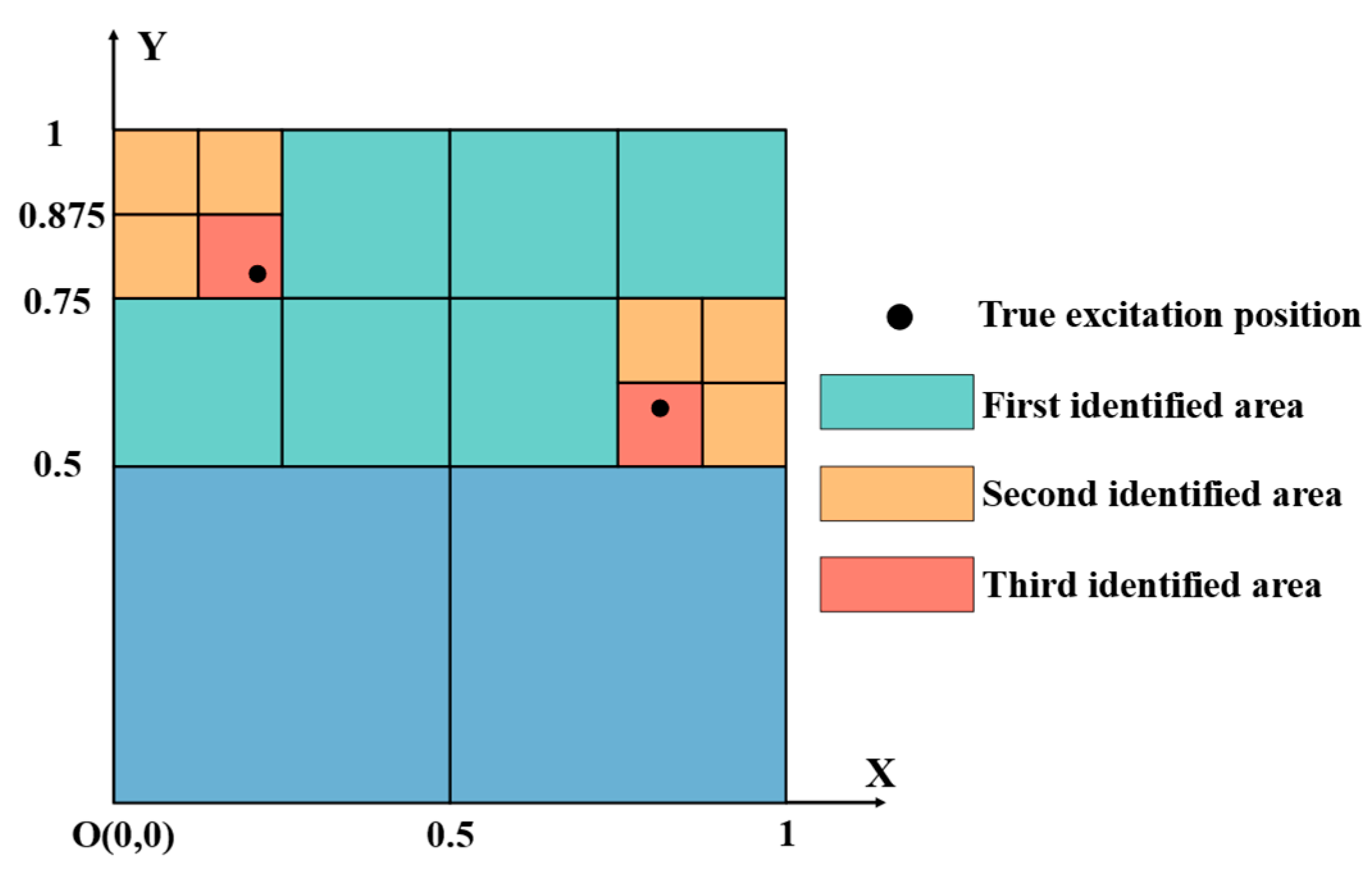
Repetition of the identification steps results in continuous approximation of the excitation positions (Figure 12).

After the completion of the identification process, the excitation positions are obtained and compared with the true excitation positions in

Table 31. Excitation positions.

		Step-By-Step Recognition Method	True Value	${\mathit{\eta }}_{\mathit{e}\mathit{r}\mathit{r}\mathit{o}\mathit{r}}$/%
$f_1$	x/m	0.1875	0.2	1.25
	y/m	0.8125	0.8
$f_2$	x/m	0.8125	0.8	2.5
	y/m	0.5625	0.6

.

Table 31 demonstrates some errors in step-by-step identification, but it basically meets the requirements of location identification accuracy in engineering practice. In order to obtain a more accurate solution, the number of identification steps can be increased, until the required precision is achieved.

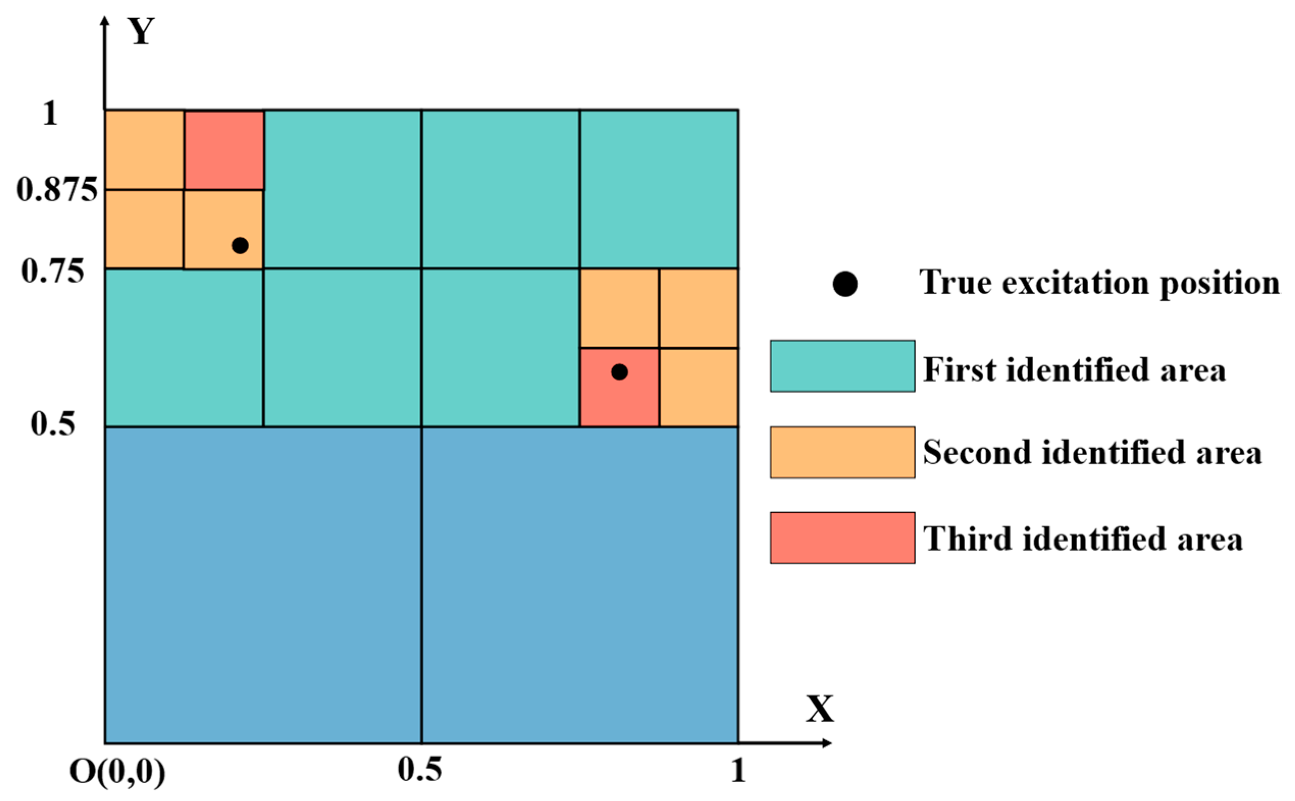
When the dynamic response contains 10% noise, under operational condition 1 (with four dynamic response measurement points on the structure), one of the dynamic load locations is incorrectly identified during the third identification process. The identification process is illustrated in Figure 13.

In this case, the recognition error for multi-point dynamic loads is larger compared to previous operational condition. The main error is attributed to the mistake in the final recognition process. The specific recognition errors are presented in

Table 32. Excitation positions of multi-point dynamic loads with 10% noise under operating condition 1.

		Step-By-Step Recognition Method	True Value	${\mathit{\eta }}_{\mathit{e}\mathit{r}\mathit{r}\mathit{o}\mathit{r}}$/%
$f_1$	x/m	0.1875	0.2	7.5
	y/m	0.9375	0.8
$f_2$	x/m	0.8125	0.8	2.5
	y/m	0.5625	0.6

.

4.2.5. Computational Time for the Identification of Multi-Point Dynamic Loads

When considering two dynamic loads on the same structure, traditional methods require randomly selecting two mesh nodes on the structure for combination. This combination increases rapidly as the number of meshes increases. In contrast, the method proposed in this paper only requires selecting a small number of nodes for identification at each step.

Under operational condition 1, two virtual loads are applied and four virtual accelerations are measured for each identification, in the first step, the virtual loads are applied to 12 virtual excitation points, and 24 response data points are measured. This requires the total of 24 dynamic response data to be measured. Subsequently, at each sub-step, 32 virtual excitations are applied, and 64 dynamic responses are measured. Across three steps, 76 virtual excitations are required to measure 152 dynamic responses. Under operational condition 2, two virtual loads are applied and nine virtual accelerations are measured for each identification, in the first step, the virtual loads are applied to 12 virtual excitation points, and 54 response data points are measured. This requires the total of 54 dynamic response data to be measured. Subsequently, at each sub-step, 32 virtual excitations are applied, and 144 dynamic responses are measured. Across three steps, 76 virtual excitations are required to measure 342 dynamic responses. In comparison, the general method will result in a total of ${\mathrm{C}}_{441}^2=97020$ combinations, which necessitate $2\cdot {\mathrm{C}}_{441}^2$ virtual loads and $4\cdot {\mathrm{C}}_{441}^2$ dynamic response measurements under operational condition 1, and $9\cdot {\mathrm{C}}_{441}^2$ dynamic response measurements under operational condition 2.

Therefore, this method apparently significantly reduces the calculation time and increases solving efficiency compared to the general dynamic load identification method.

Table 33. Comparison of computation for identification of multi-point dynamic loads between traditional and step-by-step methods.

	Number of Applied Loads	Number of Response Data	Number of Loads Applied in Traditional Method	Number of Responses Collected in Traditional Method
Step 1	12	24/54	$2\cdot {\mathrm{C}}_{441}^2$	$4\cdot {\mathrm{C}}_{441}^2/9\cdot {\mathrm{C}}_{441}^2$
Step 2	44	88/198
Step 3	76	152/342

shows the number of virtual loads that should be applied and the number of measured responses in the traditional method and the method used in this paper.

5. Experimental Verification

5.1. Thin Plate Modal Test

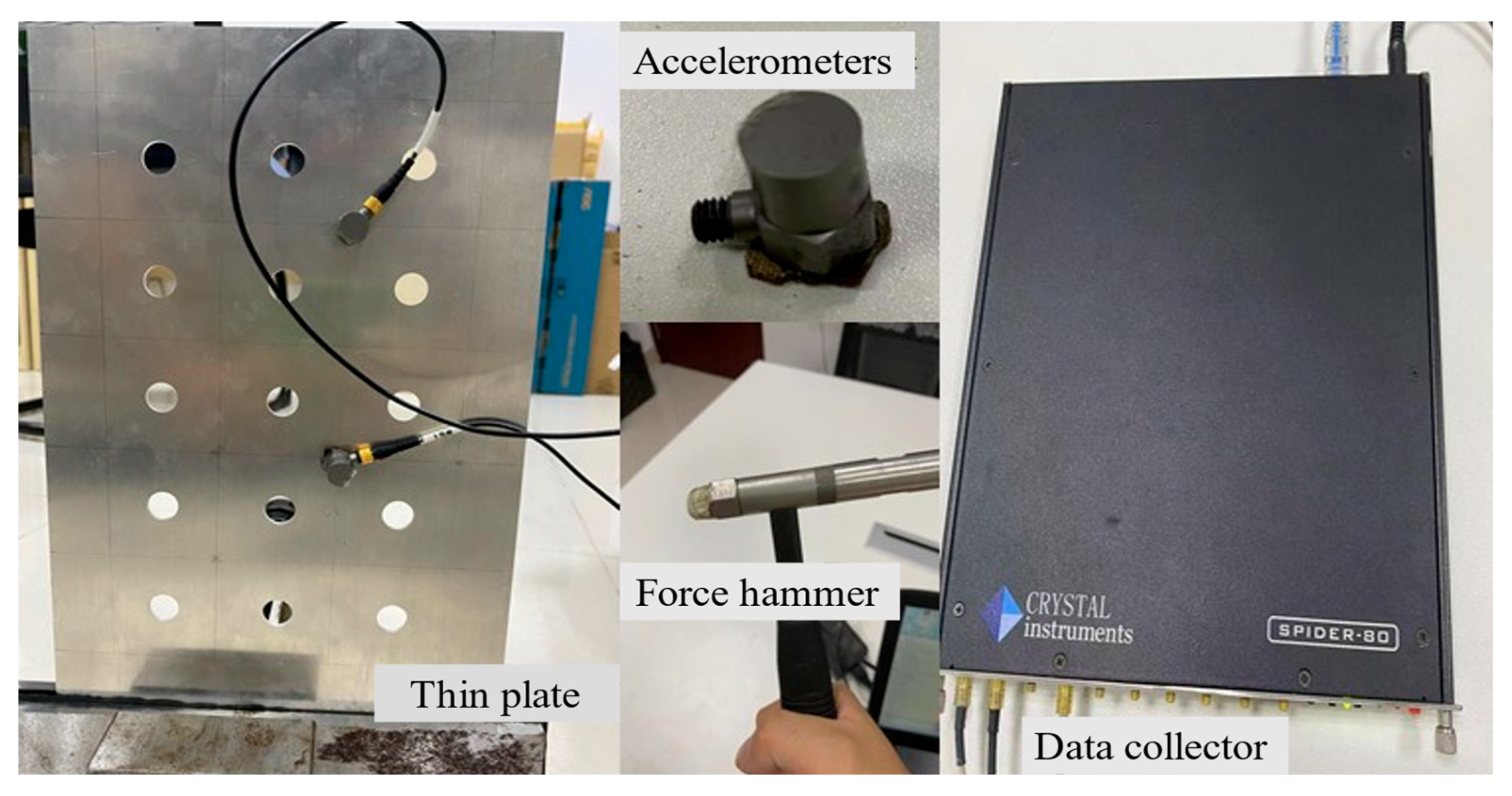
A rectangular thin plate with holes is used as a test piece to verify the step-by-step identification method. The thin plate measures 0.3 m in length, 0.2 m in width, and 0.002 m in thickness. The test equipment is depicted in Figure 14.

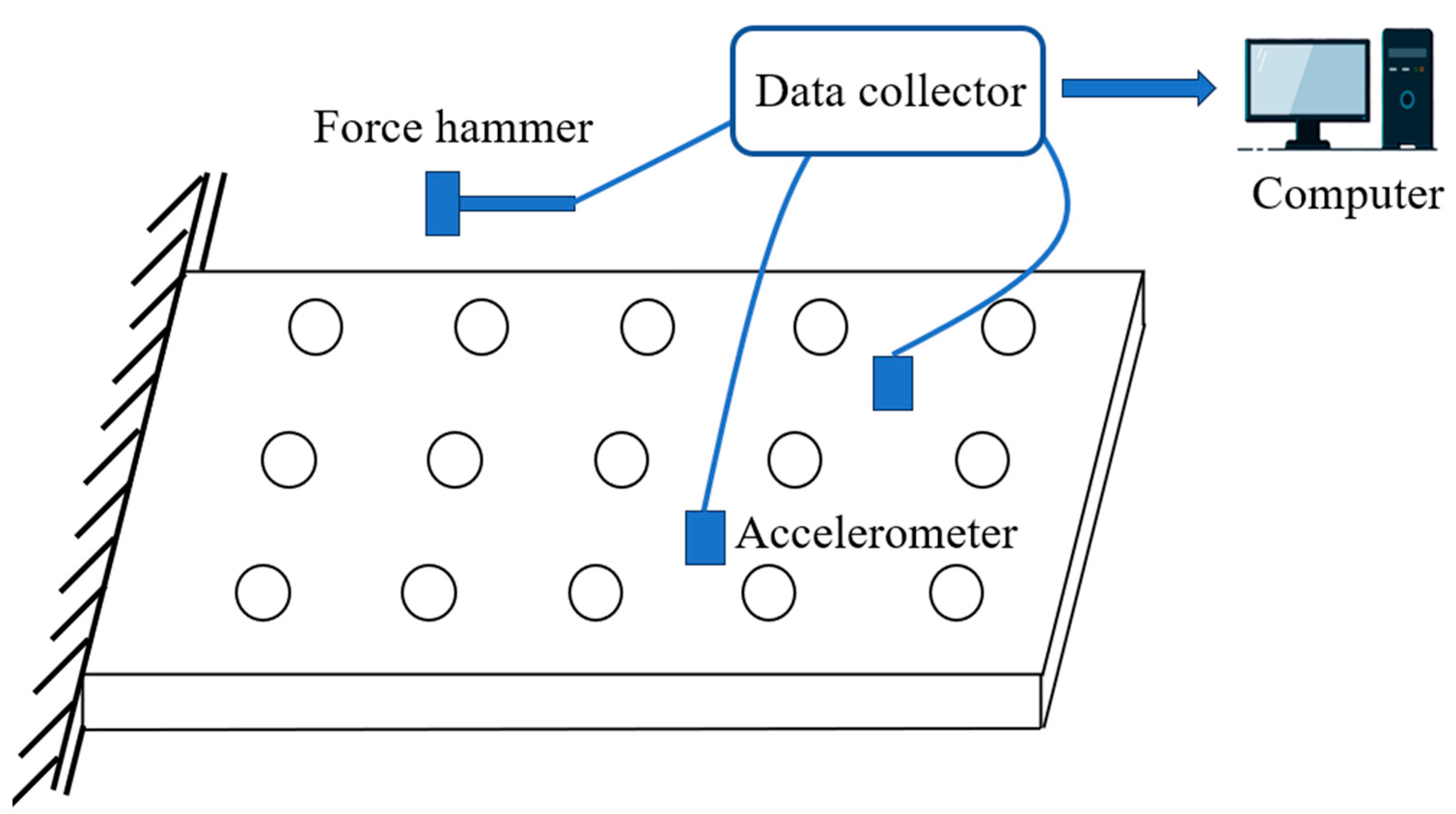
The three sides of the test plate with holes are free, while the fourth side is fixed. During the experiment, accelerometers are attached to the thin plate, and a force hammer is used to strike it. The data collected from both the force hammer and the accelerometers are transmitted to a data collector, which then sends the data to a computer. The corresponding software is used to process the data, enabling the successful execution of the experiment. A detailed schematic of the experimental setup is shown in Figure 15.

The model is adjusted according to the natural frequencies measured during the thin plate test to ensure similarity between the first three natural frequencies of the model and the test results. The measured natural frequencies and the adjusted natural frequencies are presented in

Table 34. The first 4 orders of the natural frequency of sheet metal (in Hz).

Modes Order	1	2	3	4
Experimental data	18.0	62.5	112.5	204
Modal modification	18.5	61.5	114.8	207.9

.

Finite-element model correction is typically performed after the first few natural frequencies of the structure have been measured experimentally, with the goal of minimizing the discrepancy between the finite-element simulation and the experimental data. Due to factors such as manufacturing errors, modeling inaccuracies, material inhomogeneity, or environmental effects, the experimentally measured natural frequencies of the structure may differ from those calculated by the finite-element software.

After modification of the finite-element structural parameters according to the test data, the adjusted natural frequency is similar to the natural frequency measured in the test, and the next step of dynamic load identification can be carried out.

5.2. Identification Process

The coordinate system of the thin plate is given in Figure 16. An impact load is applied at the point (0.225 m, 0.075 m), and two response points are selected, located at (0.225 m, 0.125 m) and (0.125 m, 0.125 m), respectively.

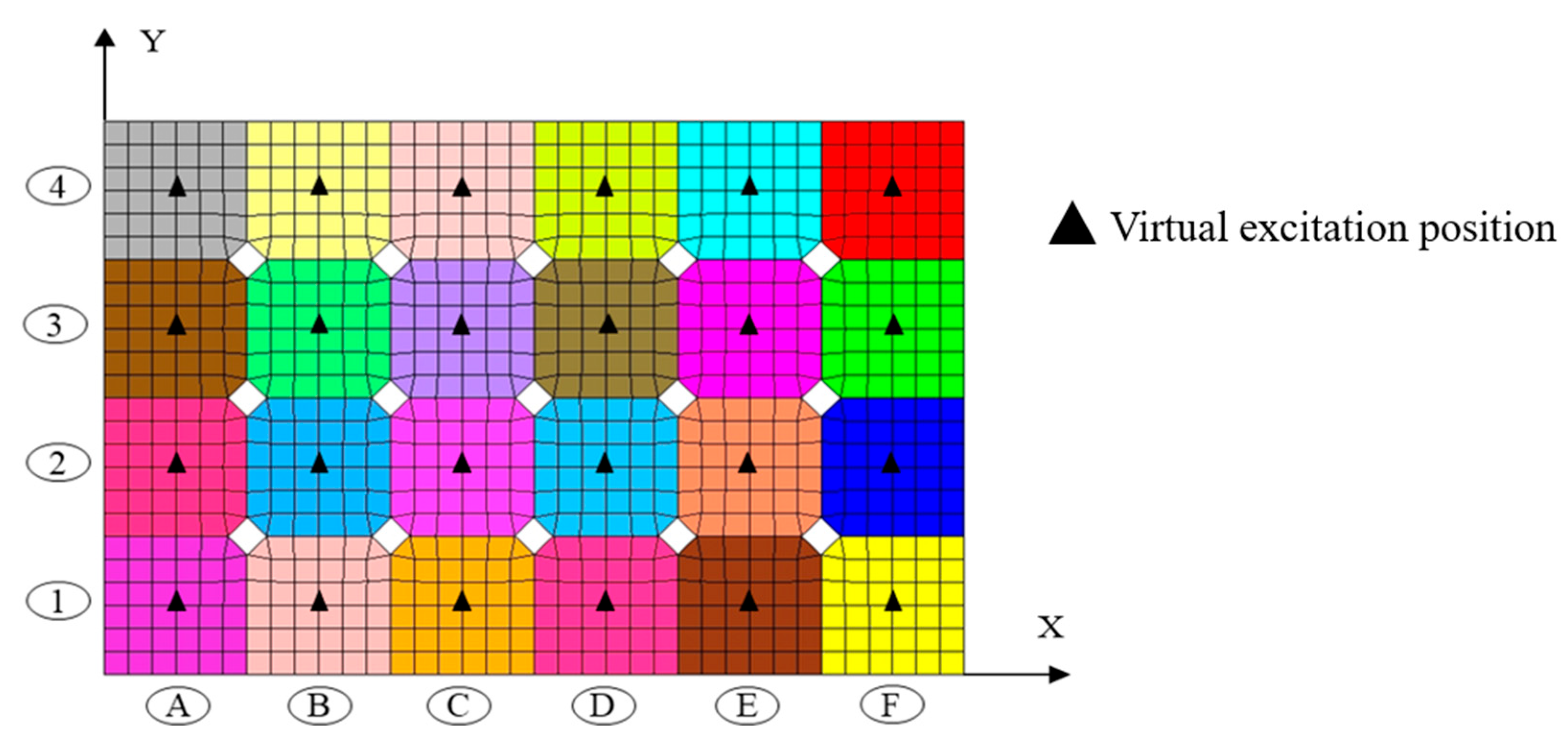
The finite-element model of the thin plate is developed, divided into 24 regions (denoted with different colors) in Figure 17. Subsequently, a virtual excitation point is selected within each area, and a unit impact load is applied at these virtual excitation positions using the software. The locations of the selected response points correspond to those of the response points in the test model.

The black triangles indicate the locations of the selected virtual excitation points. To simplify identification, each region of the plate is labeled. The acceleration data at the response points are obtained by applying a unit load at the virtual excitation point. The correlation metrics are calculated between these responses and the test acceleration data, as shown in

Table 35. Correlation metrics for first identification for various regions.

	A	B	C	D	E	F
1	0.9069	0.9260	0.9386	0.9454	0.9478	0.9479
2	0.9267	0.9361	0.9444	0.9492	0.9503	0.9495
3	0.9171	0.9290	0.9397	0.9467	0.9487	0.9482
4	0.8786	0.9071	0.9269	0.9383	0.9430	0.9442

.

The highest correlation metric is for region E2 indicating that the impact load during the test is located in this region. Subsequently, the finite-element model of this region is further divided into smaller sub-regions, with appropriate labeling (Figure 18).

For the second identification, the correlation metrics between the acceleration responses under virtual excitation and the experimental acceleration data are presented in

Table 36. Correlation metrics for second identification for various regions.

	A	B	C
1	0.9532	0.9534	0.9533
2	0.9536	0.9537	0.9536
3	0.9534	0.9535	0.9534

.

It is evident from Table 36 that the correlation metric of region B2 is the highest. Therefore, it can be inferred that the test impact load is situated in this region (0.225 ± 0.0083 m, 0.075 ± 0.0083 m), with the minimal difference between the identified and actual positions (0.225 m, 0.075 m). Subsequent subdivision of the finite-element model could further enhance accuracy. However, the correlation metrics in region B2 are already quite close. This is attributed to the small element size relative to the thin plate in Figure 18.

Since the test thin plate model is relatively simple, with fewer finite-element nodes, the entire model mesh can be subdivided into finer elements. But there is no need to refine the finite-element mesh in the subsequent stages of the identification process. In contrast, models of actual engineering structure are complex, allowing a coarse initial finite-element mesh. After determining the initial location region, only the local mesh needs refinement to avoid excessive remeshing of the overall model, which could complicate the calculations.

6. Conclusions

At the outset of this paper, a formula for the calculation of the correlation coefficient for dynamic responses is presented. Various types of virtual loads are discussed in relation to different dynamic load scenarios. It is observed that all types of dynamic loads can be characterized in terms of a single-point dynamic load with a single frequency or a multi-point dynamic load with a single frequency for identification purposes. Subsequently, in simulations, the effectiveness of this method was verified through the identification of single-point and two-point dynamic loads with different noise magnitudes and sensor numbers. In practical experiments, the method proposed in this study is employed to ascertain the spatial distribution of dynamic loads on thin plates, meeting the accuracy requirements for engineering applications. Consequently, the following conclusions can be drawn:

• By applying the method of step-by-step identification, the identification of dynamic load location can be changed from applying virtual loads on each node on the finite-element model to their use on some nodes step-by-step, greatly reducing the simulation.
• Numerical studies and experimental results show that, for a single dynamic load, its location can be accurately identified even with 10% noise in the response and only four sensors, with a location identification error of 1.25%.
• For two-point dynamic loads, when the response contains 10% noise, the structure with only four sensors results in a 7.5% error in the identification of one of the dynamic load locations. However, with nine sensors, the location can be accurately identified, reducing the error to 1.25%.

However, the step-by-step identification method also has some shortcomings. For special load locations, for instance, when the distance between multiple dynamic loads is too small, it may not be able to accurately identify multiple dynamic loads since they cannot be distinguished in the first step. At the same time, it is necessary to know the number of dynamic loads in advance when identifying multi-point dynamic loads. These will be the key points for future research on the identification of dynamic load positions.

References

1. Chen, Z.; Chan, T.; Nguyen, A.; Yu, L. Identification of vehicle axle loads from bridge responses using preconditioned least square QR-factorization algorithm. Mech. Syst. Signal Process. 2019, 128, 479–496. [Google Scholar] [CrossRef]
2. Park, J.; Ha, S.; Chang, F. Monitoring impact events using a system-identification method. AIAA J. 2009, 47, 2011–2021. [Google Scholar] [CrossRef]
3. Giannopoulos, I.; Georgantzinos, K. Establishing detection maps for carbon nanotube mass sensors: Molecular versus continuum mechanics. Acta Mech. 2017, 6, 2377–2390. [Google Scholar] [CrossRef]
4. Bartlett, F.; Flannelly, W. Model verification of force determination for measuring vibratory loads. J. Am. Helicopter. Soc. 1979, 24, 10–18. [Google Scholar] [CrossRef]
5. Qin, Y.; Zhang, Y.; Silberschmidt, V. Distributed dynamic load in structural dynamics by the impulse-based force estimation algorithm. Comput. Model. Eng. Sci. 2024, 139, 2865–2891. [Google Scholar] [CrossRef]
6. Jiang, J.; Cui, W.; Chen, S.; Guo, X.; Zhao, J. A novel dynamic load identification method based on improved basis functions and implicit Newmark for continuous system with unknown initial conditions. Mech. Syst. Signal Process. 2024, 208, 110987. [Google Scholar] [CrossRef]
7. Rezayat, A.; Nassiri, V.; Pauw, D.; Ertveldt, J.; Vanlanduit, S.; Guillaume, P. Identification of dynamic forces using group-sparsity in frequency domain. Mech. Syst. Signal Process. 2016, 70–71, 756–768. [Google Scholar] [CrossRef]
8. Li, K.; Xiao, L.; Liu, M.; Kou, Y. A distributed dynamic load identification approach for thin plates based on inverse Finite Element Method and radial basis function fitting via strain response. Eng. Struct. 2025, 322, 119072. [Google Scholar] [CrossRef]
9. Liu, Y.; Wang, L.; Feng, B. A hybrid model-data-driven framework for inverse load identification of interval structures based on physics-informed neural network and improved Kalman filter algorithm. Appl. Energy 2024, 359, 122740. [Google Scholar] [CrossRef]
10. Prawin, J.; Rao, A. An online input force time history reconstruction algorithm using dynamic principal component analysis. Mech. Syst. Signal Process. 2018, 99, 516–533. [Google Scholar] [CrossRef]
11. Zhang, C.; Zhang, W.; Ying, G.; Ying, L.; Hu, J.; Chen, W. A deep learning method for heavy vehicle load identification using structural dynamic response. Comput. Struct. 2024, 297, 107341. [Google Scholar] [CrossRef]
12. Wang, L.; Xu, H.; Liu, Y. A novel dynamic load identification approach for multi-source uncertain structures based on the set-theoretical wavelet transform and layered noise reduction. Structures 2023, 51, 91–104. [Google Scholar] [CrossRef]
13. Wang, C.; Chen, D.; Chen, J.; Lai, X.; He, T. Deep regression adaptation networks with model-based transfer learning for dynamic load identification in the frequency domain. Eng. Appl. Artif. Intell. 2021, 102, 104244. [Google Scholar] [CrossRef]
14. Zhou, R.; Qiao, B.; Liu, J.; Chen, W.; Chen, X. Impact force localization and reconstruction via gated temporal convolutional network. Aerosp. Sci. Technol. 2024, 144, 108819. [Google Scholar] [CrossRef]
15. Zhou, J.; Dong, L.; Guan, W.; Yan, J. Impact load identification of nonlinear structures using deep Recurrent Neural Network. Mech. Syst. Signal Process. 2019, 133, 106292. [Google Scholar] [CrossRef]
16. Zhang, J.; Zhang, F.; Jiang, J. Research on load position identification technology using separated variable method. J. Vib. Eng. 2021, 34, 584–591. [Google Scholar]
17. Chen, B.; Hei, C.; Luo, M.; Song, G. Pipeline two-dimensional impact location determination using time of arrival with instant phase (TOAIP) with piezoceramic transducer array. Smart Mater. Struct. 2018, 27, 105003. [Google Scholar] [CrossRef]
18. Zhao, G.; Hu, H.; Li, S.; Liu, L.; Li, K. Localization of impact on composite plates based on integrated wavelet transform and hybrid minimization algorithm. Compos. Struct. 2017, 176, 234–243. [Google Scholar] [CrossRef]
19. Jang, B.; Kim, C. Impact localization of composite stiffened panel with triangulation method using normalized magnitudes of fiber optic sensor signals. Compos. Struct. 2019, 211, 522–529. [Google Scholar] [CrossRef]
20. Simone, M.; Ciampa, F.; Meo, M. A hierarchical method for the impact force reconstruction in composite structures. Smart Mater. Struct. 2019, 28, 085022. [Google Scholar] [CrossRef]
21. Ciampa, F.; Meo, M. Impact localization on a composite tail rotor blade using an inverse filtering approach. J. Intell. Mater. Syst. Struct. 2014, 25, 1950–1958. [Google Scholar] [CrossRef]
22. Liu, Q.; Wang, F.; Liu, M.; Xiao, W. A two-step localization method using wavelet packet energy characteristics for low-velocity impacts on composite plate structures. Mech. Syst. Signal Process. 2023, 188, 110061. [Google Scholar] [CrossRef]
23. Qin, Y.; Zhang, Y.; Silberschmidt, V.; Zhang, L. Method for dynamic load location identification based on FRF decomposition. Aerospace 2023, 10, 852. [Google Scholar] [CrossRef]
24. Thiene, M.; Sharif, K.; Aliabadi, M. Comparison of artificial neural networks and the transfer function method for force reconstruction in curved composite plates. Key Eng. Mater. 2014, 627, 301–304. [Google Scholar] [CrossRef]
25. Wen, X.; Sun, Q.; Li, W.; Ding, G.; Song, C.; Zhang, G. Localization of low velocity impacts on CFRP laminates based on FBG sensors and BP neural networks. Mech. Adv. Mater. Struct. 2022, 29, 5478–5487. [Google Scholar] [CrossRef]
26. Liu, Q.; Wang, F.; Li, J.; Xiao, W. A hybrid support vector regression with multi-domain features for low-velocity impact localization on composite plate structure. Mech. Syst. Signal Process. 2021, 154, 107547. [Google Scholar] [CrossRef]
27. Yan, D.; Hu, Y.; Lang, L. Bending load monitoring and positioning method of long-span composite structures. Chin. Mech. Eng. 2023, 34, 2257–2267. [Google Scholar]
28. Liu, J.; Qiao, B.; Chen, Y.; Zhu, Y.; He, W.; Chen, X. Impact force reconstruction and localization using nonconvex overlapping group sparsity. Mech. Syst. Signal Process. 2022, 162, 107983. [Google Scholar] [CrossRef]
29. Giannopoulos, I. Crack Identification in Graphene Using Eigenfrequencies. Int. J. Appl. Mech. 2017, 9, 18. [Google Scholar] [CrossRef]
Figure 1. Preliminary calibration diagram of thin plate.
Aerospace 12 00953 g001
Figure 2. Selection diagrams of virtual load points for different structures.
Aerospace 12 00953 g002
Figure 3. Result of the first identification when the loads are too close.
Aerospace 12 00953 g003
Figure 4. Flowchart of multi-point identification of dynamic loads with multiple frequencies.
Aerospace 12 00953 g004
Figure 5. Model for first identification.
Aerospace 12 00953 g005
Figure 6. Model for second identification.
Aerospace 12 00953 g006
Figure 7. Flow chart for stepwise identification.
Aerospace 12 00953 g007
Figure 8. Position of the acceleration sensors under two operational conditions.
Aerospace 12 00953 g008
Figure 9. Location of excitation and response points.
Aerospace 12 00953 g009
Figure 10. Step-by-step identification diagram.
Aerospace 12 00953 g010
Figure 11. Locations of excitation and response points on thin plate.
Aerospace 12 00953 g011
Figure 12. Step-by-step identification diagram for multi-point dynamic load case.
Aerospace 12 00953 g012
Figure 13. Identification results of multi-point dynamic loads with 10% noise under operating condition 1.
Aerospace 12 00953 g013
Figure 14. Schematic diagram of sheet test.
Aerospace 12 00953 g014
Figure 15. Experimental schematic diagram of a thin plate with round holes.
Aerospace 12 00953 g015
Figure 16. Plane coordinates for test with thin plate.
Aerospace 12 00953 g016
Figure 17. Finite-element model of thin plate for first identification.
Aerospace 12 00953 g017
Figure 18. Finite-element model of region E2 of thin plate for second identification.
Aerospace 12 00953 g018