Abstract
In this study, experiments and numerical simulations were conducted to investigate the oscillation phenomena in a pressure swirl injector. The flow field was captured using high-speed photography, and the gray values were analyzed using the Matlab image processing program. The oscillation frequency was recorded using FFT transform. Additionally, the flow field of the pressure swirl injector was simulated based on the volume of fluid (VOF) interface-tracking method. Both the experimental and numerical results revealed periodic oscillations in the pressure swirl injector, with a corresponding frequency of several hundred Hertz. The oscillation frequency is closely related to the behavior of the central gas core, which has greater turbulent kinetic energy than the liquid phase. As the mass flow rate increases, the velocity of the gas core is increased. The turbulent kinetic energy of the central gas core increased, which led to an increase in the oscillation frequency. Finally, the relationship between Re and the oscillation frequency was obtained.
1. Introduction
Pressure swirl injectors, which produce a hollow cone spray, are widely utilized in liquid rocket engines, gas turbine engines, and boilers due to their excellent atomization characteristics. The liquid enters from the tangential slots on the swirl chamber with a certain tangential velocity and then moves spirally downward. After passing through the convergent section, the liquid velocity increases significantly and expands along the radial direction. This results in the formation of a spray cone after leaving the injector. The gas enters the injector under the influence of a pressure difference between the inside and outside of the injector [1,2].
The phenomenon of oscillation in the pressure swirl injector has been confirmed by research. Horvay and Leuckel [3] were the first to measure the flow field inside the pressure swirl injector. They used a mixture with the same refractive index as plexiglas and determined the axial and tangential velocities inside the injector using a Laser Doppler Anemometer (LDA). Pulsations were observed in both the axial and tangential velocities, which were attributed to velocity pulsations caused by turbulence within the injector. Chinn [4] asserted that velocity fluctuation was due to instability in the gas core. Wang Zhiren [5] likened the flow inside the injector to shallow water waves in an open groove and deduced a frequency formula for vibration within the injector. Zhou Jin et al. [6] and Huang Yuhui et al. [7] studied the self-excited oscillation of coaxial centrifugal injectors in YF-75 engines, concluding that it resulted from resonance between central air vortexes and the airflow in gas channels. Ma [8] measured axial and tangential velocities inside injectors using LDA with water as the medium; the results suggested an oscillation phenomenon with a frequency of 100 Hz within injectors. Marchione [9] utilized a light source and CCD camera to observe the spray morphology of a conical liquid film from a pressure swirl injector injecting into a static atmosphere. Two different oscillation frequencies were identified through FFT transformation: one ranging from 100 to 125 Hz, and another exhibiting high-frequency oscillations at 1800 Hz.
Xue Shuaijie et al. [10] discovered that the open-type centrifugal injector exhibited a self-excitation oscillation phenomenon with a frequency of 10–40 Hz, and the internal gas core periodically displayed “discontinuity” and “continuity”, leading to a wrinkling and accumulation phenomenon similar to the Klystron effect. The self-excited oscillation may be attributed to the interaction between the liquid film flow and gas core oscillation in the swirl chamber. Chinn et al. [11] and Maly et al. [12] conducted numerical simulations and experimental research on centrifugal nozzles with different structures, revealing periodic oscillations in the internal gas core at frequencies around tens of Hz. Additionally, Zhang Xinqiao [13] designed and processed a transparent centrifugal nozzle, observing high-frequency oscillations ranging from 1100 Hz to 2200 Hz in the gas core within the swirl chamber. Moreover, it was noted that the oscillation frequency increased as the Reynolds number at the liquid inlet rose, with the characteristics of the gas core oscillation considered as indicative of changes in rotation speed within the swirl chamber. Furthermore, Cheng Peng [14] found that inner flow parameters such as the air core diameter and axial velocity fluctuate due to pressure variations in the supply system at driving frequency. G. Arun Vijay et al. [15] conducted a comprehensive review of the literature on the flow inside and outside the pressure swirl injector and pointed out that the flow inside nozzles is turbulent and unsteady. Researchers [16,17,18,19] have used numerical simulation and indicated the unsteady flow character inside the injector and its influence on liquid sheet formation. More studies on the oscillation characteristics in pressure swirl injectors can be found in [20].
Although the instability of the simplex swirl injectors has been verified through experiments and simulations, the mechanism of the instability still needs further exploration. Due to the significant influence of the internal flow process on the liquid film fragmentation, the internal flow of the injector needs to be studied more thoroughly [21]. With the improvement in optical measurement techniques and the enhancement of numerical simulation methods, more detailed research has become feasible. In this study, a transparent injector was designed for the purpose of investigating the internal flow field using high-speed photography. Following image processing, the gray values of the image inside and outside the injector were subjected to FFT transformation, allowing for determination of the periodic frequency of the gray value within the image. In order to elucidate the reason for the oscillation phenomena, numerical simulations of the flow field within the injector were conducted utilizing a VOF method coupled with N-S incompressible equations. Furthermore, an investigation of the flow field is performed to explain the oscillation phenomenon in the pressure swirl injector.
2. Experimental Setup and Numerical Model
2.1. Experimental Setup
The structure of the injector can be divided into three parts: the swirl chamber, the convergent section, the central post, and the divergent section (as shown in Figure 1). The geometric parameters of the injector are listed in Table 1. The diameters of the swirl chamber, the central post, and the tangential slot are 10.2 mm, 4.7 mm, and 2.0 mm respectively. A transparent injector was constructed using various transparent modules that were individually designed and machined [13,14], as shown in Figure 2.
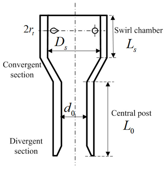
Figure 1.
Sketch map of pressure swirl injector.

Table 1.
The geometric parameters of the pressure swirl injector.

Figure 2.
The transparent injector.
The velocity at the tangential slot and the Reynolds number could be determined using Formulas (1) and (2).
where , , and represent the mass flow rate, the density, and the kinetic viscosity of liquid fuel, respectively. rt and d0 represent the radius of the tangential slots and the diameter of the central post, respectively. The mass flow rate was maintained at 232.25 g/s during the test. As the area of the tangential hole is 3.14 mm2, the velocity at the inlet was 18.5 m/s and the Reynolds number was 86,517, according to Formulas (1) and (2).
Two points, point B and point C, located outside and inside the injector, respectively, were chosen for studying the change in Mie scattering intensity. The experimental principle is depicted in Figure 3. A uniform light source is emitted from a camera lamp and filtered through depolished glass. High-speed photography was utilized to capture the instantaneous flow field at a capturing frequency of 8000 fps and with an exposure time of 1/8000 s. Each image had dimensions of 1024 by 1024 pixels. Finally, the spray image was obtained, as shown in Figure 2. Using the image processing functions of Matlab, the grayscale values of each point on the image were obtained. By performing an FFT transformation on the gray values, the spectral information was obtained.

Figure 3.
Schematic of experimental setup.
2.2. Numerical Model and Grid Independence Validation
Gas and liquid phases coexist within the interior of the injector, and the interface tracking method [22,23,24,25] plays a crucial role in the numerical simulation of gas–liquid two-phase flow. By utilizing the VOF model and the incompressible Navier–Stokes equation, it is possible to solve for the flow field inside the pressure swirl injector. Specifically, in order to utilize a structured grid, the tangential circular inlet was considered equivalent to a 1.57 mm2 square inlet in the simulation. The size of this equivalent square slot along the axial direction was set to be equal to the diameter of the tangential slots.
The governing equations for the incompressible Navier–Stokes equations are as follows:
where represents the velocity in grid i and is the surface tension of the gas–liquid interface
where represents the volume fraction of liquid phase in the computed cell. These cases should be considered when one of the following conditions is met:
, besides , or
, besides
The transport equation of the volume content of the liquid phase is as follows:
The density and the viscosity of each cell in the mixture region should be calculated as follows:
The following are the descriptions of the boundary conditions.
At the inlet of the swirl chamber, the velocity was specified as 18.5 m/s and the mass flow rate was 232.25 g/s. Water was used as the simulation medium, with a turbulent intensity of 5%. At the exit of the injector, pressure was specified as 1 atm and the turbulent intensity was increased to 10%. The wall boundary condition was set as a non-slip stationary wall. Gravity effects on water were taken into account, and the surface tension was considered to be 0.07237 N/m. The turbulence model employed in this study was the RNG k-e model, which is known for its effectiveness in modeling strong swirl flow. A non-equilibrium wall function was employed to simulate the flow field near the wall. The unsteady formulation used in this simulation was a first-order implicit method with a time step of 5 × 10⁻⁵ s. The initial liquid content at the beginning of simulation was 0. Additionally, numerical simulation monitored the liquid content of grid G (as shown in Figure 2) and the average total pressure of the tangential slot; the oscillation frequency was then obtained through FFT analysis.
The static pressure at the tangential slot and the liquid content at grid G were calculated to compare the grid resolution. Three different grids were utilized for this comparison, specifically 108 × 26 × 117, 128 × 30 × 140, and 156 × 37 × 175. The static pressure at the inlet and the liquid content at grid G were monitored; the average results are listed in Table 2. Taking the results of the 156 × 37 × 175 grid as the standard, the errors of static pressure and the liquid content at grid G are 8% and 7.6%, respectively, using the 108 × 26 × 117 grids. While the errors using the 128 × 30 × 140 grids are below 5%. Taking the computing costs into account, the 128 × 30 × 140 grid was selected as the calculation grid, as shown in Figure 4.
Table 2.
Validation of grid independence.
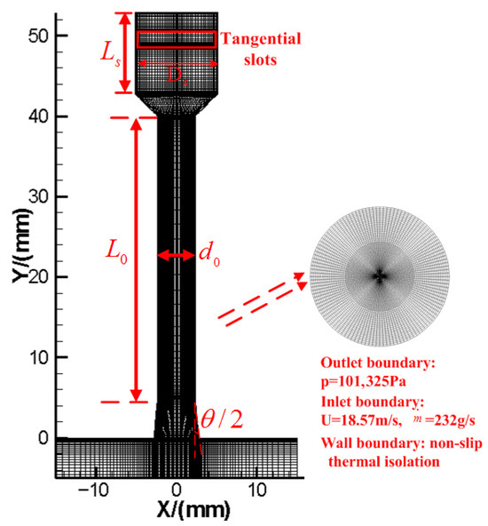
Figure 4.
Grid configuration of the injector.
There are two more steps for verifying the reliability of the calculation results.
Figure 5 shows the tangential velocity in the swirl chamber from numerical results. The liquid phase velocity exists at the location where the water fraction is equal to 1, that is, within the area enclosed by the dotted line in the figure. The numerical results and the experimental results from Ma [8] are compared in Figure 6. Ma [8] obtained experimental results using LDV, which only reflects the speed of the liquid phase. The calculated results are obtained from theoretical calculation [8]. The numerical results are closest to those of Experiment 3 in the liquid phase. At the position of 0.45 times the radius, the error reaches its maximum, ranging from 10.5% to 11.7%. From 0.8 times the radius to the wall, the velocities of both the numerical results and the experimental results from Ma [8] are almost the same.
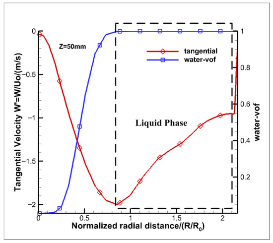
Figure 5.
The tangential velocity in the swirl chamber from numerical results.
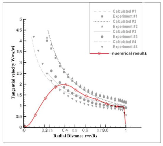
Figure 6.
The comparison between the numerical results and experimental results from Ma [8].
The mean spray angle, as calculated from the computations, was also determined. Figure 7 shows the spray cone angle of 52.38° from the simulation results. Figure 8 shows the spray cone angle of 59°obtained by the image processing of the spray image under the same operating conditions. The two results also align well. Research on the spray cone angle can be found in [26].
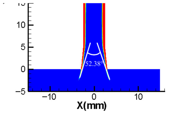
Figure 7.
Spray cone angle from numerical results: 52.38°.

Figure 8.
Spray cone angle from experimental results: 59.6°.
3. Results and Discussion
3.1. Experimental Results
The internal flow images of the injector, captured by high-speed photography, are shown in Figure 2. Based on the image processing function of Matlab, the original image was transformed into a grayscale image with values ranging from 0 to 255. The changes in the gray values of points B and C over time were obtained, as shown in Figure 9a and Figure 9b, respectively. The average gray level in the swirl chamber is approximately 55, while it is about 50 outside the injector—slightly lower than that within the swirl chamber. This difference is attributed to the curvature of the injector and variations in refractive indices of water, quartz, and air [13]. Following FFT transformation, the oscillation frequencies of points B and C were determined, as depicted in Figure 9c. Both points B and C exhibit periodic changes in gray values with a frequency of 100 Hz. This frequency aligns with the findings from Marchione [9], indicating that the spray field of the pressure swirl injector is characterized by an oscillation phenomenon at a frequency of 100 Hz.
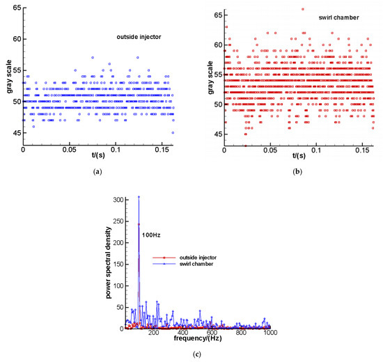
Figure 9.
(a) Gray scale of point B. (b) Gray scale of point C. (c) FFT frequency from the experiments.
3.2. Numerical Results
In order to study the internal flow field of the injector, a model of the same size as the experimental injector was established and numerical simulation results were obtained using the numerical method discussed in Section 2.2.
During the simulation process, some parameters were monitored, and the changes in these parameters over time were obtained. Periodic signals were obtained by performing FFT transformation on these parameters. Figure 10a is the liquid content of grid G. The average liquid fraction at grid G is 0.16, and the amplitude of the liquid fraction is 150%. Figure 10b is the spectrum information obtained through FFT transformation over 15 timesteps, revealing periodic changes of 400 Hz. The pressure at the tangential slot was also monitored, which is omitted from this list. The average pressure is 1.475 MPa, and the amplitude of pressure vibration is 2%. Also, the FFT result shows periodic changes of 400 Hz.
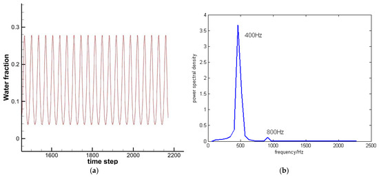
Figure 10.
(a) Liquid content at point G. (b) FFT results for liquid content.
Meanwhile, variation in the gas core diameter inside the swirl chamber was analyzed. Figure 11 illustrates the gas–liquid distribution in the Y = 47 mm plane that lies in the swirl chamber. The blue region in the center represents the gas core, while the surrounding area is occupied by the liquid phase. At the gas–liquid interface, the liquid volume c equals 0.5. The variation in the radius of the gas core over several cycles was recorded; finally, a periodic sinusoidal change was obtained, as listed in Formula (9).
where “r” represents the instantaneous radius of the gas core, “r0” denotes the average radius of the gas core, “w” denotes the angular frequency, and φ0 is the initial phase.
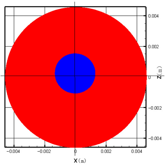
Figure 11.
Gas–liquid distribution in the Y = 47 mm plane (liquid phase—red region, gas core—blue region).
The radius in different planes and the parameters in Formula (9) are recorded in Table 3, where the value of “Y” represents the position of the gas core. Y = 12 mm and Y = 40 mm are located in the central post, while Y = 45 mm is located in the swirl chamber. It can be deduced that the diameter of the gas core is larger in the central post than in the swirl chamber. All of the diameters of the gas core exhibit an angular frequency around 2500 Hz. According to the following formula, the period of the gas core diameter is calculated to be approximately 400 Hz.
Table 3.
Parameters in Formula (9).
The period aligns with the frequency of total pressure at the tangential slot and the water content in grid G, as illustrated in Figure 10b.
The internal flow field of the injector also exhibits periodic variations. Figure 12 shows the variation process of the liquid volume fraction in the central symmetry plane. Also, the red area indicates that the volume fraction of the liquid phase c equals 1, and the blue area indicates that c equals 0. The transition zone represents different levels of the volume fraction of the liquid phase. The time interval between two adjacent pictures is 1.25 ms. In Figure 12a, the horizontal ordinate value of the center of the gas core is x < 0 in the swirl chamber. After 1.25 ms, the center of the gas core moves to the right. Finally, it returns to its initial position after 2.5 ms. It is evident that the flow field in the injector appears to be periodic. The period is calculated to be 2.5 ms, and the corresponding frequency is 400 Hz.

Figure 12.
The flow field in the central symmetry plane.
Based on the aforementioned analysis, it is evident that the internal flow field of the pressure swirl injector exhibits low-frequency oscillation characteristics, as indicated by the experimental and numerical results. Although there may be discrepancies between the frequency obtained from numerical simulation and experimental results, both sources concur that the pressure swirl injector operates with low-frequency oscillation at the given boundary conditions.
3.3. Explanations of the Oscillation Phenomenon
Numerical simulation can provide detailed flow field structures, facilitating the analysis of problems. We will provide specific details of the flow field to analyze the reasons for the internal oscillation of the injector.
Figure 13 presents the pressure, liquid phase content, and axial velocity distribution inside the swirl chamber. From the figure, the static pressure is negative at the central gas core. Under the effect of the pressure difference between the ambient atmospheric pressure and the central gas core, the gas enters the interior of the injector. It can be observed that the axial velocity direction in the central gas core region is positive, meaning that the gas core goes upward. The maximum velocity is 15 m/s. In the mixture region, the axial velocity is 0 around the gas–liquid interface, where the liquid volume fraction c equals 0.5. As the liquid volume fraction increases, the axial velocity becomes negative, meaning that the mixture moves downward. The maximum value is around 15 m/s. Figure 14 shows the static pressure at different lines. The three different lines represent the central gas core zone where x = 0, the gas–liquid mixture zone where x = 1.9 mm, and the liquid phase zone where x = 3.0 mm, respectively. The static pressure is lowest in the central gas core zone, followed by the gas–liquid mixture zone; it is highest in the liquid phase zone. The greatest pressure difference between the gas and the liquid exists in the swirl chamber. Based on the analysis above, it is evident that the gas–liquid phases exhibit distinctly different behaviors. The differences in velocity and static pressure exacerbate the interface instability.

Figure 13.
The flow field inside the swirl chamber.

Figure 14.
The static pressure at different x lines.
Figure 15 illustrates the distribution of turbulent kinetic energy at different radial positions. The turbulent kinetic energy is highest at the gas core, followed by the gas–liquid mixture zone; it is lowest in the liquid phase. Turbulent kinetic energy describes the intensity of turbulent motion, with higher levels indicating stronger turbulence. The gas phase is more unstable due to its lighter mass and smaller inertia, resulting in greater turbulent kinetic energy. The instability of the gas core leads to the instability of the gas–liquid interface and even the liquid phase.
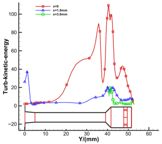
Figure 15.
The turbulent kinetic energy at different radial positions.
When the mass flow rate is raised, the internal flow field changes and the corresponding frequency changes. Figure 16 shows the static pressure of the gas core at different mass flow rates. As the mass flow rate increases, the static pressure of the gas core decreases. In relation to the results for a mass flow rate of 232 g/s, the static pressure decreases by 33% in the swirl chamber when the mass flow rate increases to 300 g/s. Figure 17 shows the turbulent kinetic energy distribution of the gas core at different mass flow rates. It was observed that a reduction in the mass flow rate effectively decreases the turbulent kinetic energy. There is a notable difference in turbulent kinetic energy around the transition area between the central post and the contraction section. When the mass flow rate is increased from 232 g/s to 300 g/s, the turbulent kinetic energy increases by 73.0%. As the turbulent kinetic energy increases, the corresponding frequency increases too. Figure 18a–c show the numerical results of the oscillation frequencies at different mass flow rates. They are 400 Hz, 685.7 Hz, and 1029 Hz at mass flow rates of 232 g/s, 250 g/s, and 300 g/s, respectively. When the mass flow rate increases from 232 g/s to 300 g/s, the oscillation frequency increases by 157%.

Figure 16.
The static pressure of the gas core at different mass flow rates.

Figure 17.
The turbulent kinetic energy at different mass flow rates.
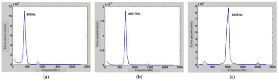
Figure 18.
The frequency at different mass flow rates. (a) The frequency when the mass flow rate is 232 g/s. (b) The frequency when the mass flow rate is 250 g/s. (c) The frequency when the mass flow rate is 300 g/s.
According to Bernoulli’s equation, when the static pressure of the gas core decreases, its velocity increases. According to Equation (11), the turbulent kinetic energy is positively correlated with its velocity. It can be deduced that as the mass flow rate increases, the turbulent kinetic energy of the gas core, as well as the oscillation frequency, is increased.
Compared with acoustic oscillation in a round tube filled with gas, the frequency can be related to the non-dimensional parameter Re, as stated in Formula (2).
In order to obtain the fitting formula, another operating condition with a mass flow rate of 200 g/s was designed, and the oscillation frequency was found to be 300 Hz. Finally, the fitting formula between the oscillation frequency and Re is
where the coefficient of determination is 0.95, as shown in Figure 19. The oscillation frequency increases as the Re number increases.
f = 4.65 × 10⁻¹³ Re 3.04

Figure 19.
The relationship between oscillation frequency and Re.
Wang [5] compared the oscillation of the liquid–gas interface to the self-pulsation of gas in a round tube and deduced the oscillation frequency to be
where K = 0, 1, 2, ……, and l is the length of the round tube.
The geometry parameter A for the base injector was 3.35, and the length of the round tube was 0.0121 m. So, the frequencies for the four different mass flow rates are 360 Hz, 466 Hz, 545.6 Hz, and 657.5 Hz, respectively. They are different from what we calculated. This is because Equation (13) is deduced based on the theory of the shallow water wave and did not consider the effect of the air core, which was only qualitatively used.
4. Conclusions
Fluctuations in the diameters of the gas core and the thickness of the liquid film produce variations in the SMD of droplets. It is closely related to the instability of combustion. In order to investigate the oscillation phenomena in a pressure swirl injector, a transparent injector was designed and assembled for this study. The instantaneous flow field was then captured using high-speed photography. After image processing, a frequency of 100 Hz was obtained. The flow field inside the injector was simulated using VOF coupled with incompressible N-S equations. Analysis of the static pressure at the tangential slot, the liquid volume fraction at the computed cell, and the radius of the gas core at different axial positions indicated a periodic oscillation of 400 Hz. Although the numerical simulation yielded a higher frequency than the experimental results, both suggested low-frequency oscillation in the pressure swirl injector. The conclusions are as follows:
- The internal flow fields inside the injectors, including velocity, pressure, and the liquid fraction at the interface, change periodically. The velocity and pressure differences between the liquid and gas phases lead to instability of the interface. The behavior of the gas core plays a significant role in the periodic variations of the entire flow field. Under the given conditions, the frequency is about several hundred Hz.
- The diameter of the gas core differs along the axial position inside the pressure swirl injector. The smallest diameter of the gas core exists in the swirl chamber of the injector and increases when approaching the exit of the injector. The oscillation amplitude of the gas core is largest in the central post section.
- As the mass flow rate at the tangential slot increases, the pressure of the gas core decreases, while its velocity rises. This leads to more intense instability, which subsequently results in a higher oscillation frequency within the injector. The fitting formula between the oscillation frequency and Re is f = 4.65 × 10⁻¹³ Re3.04.
Author Contributions
Methodology, Y.H.; Writing—original draft, J.L.; Writing—review and editing, J.L. All authors have read and agreed to the published version of the manuscript.
Funding
This work was supported by the Key Research and Development Promotion Special Project (Science and Technology Research Project) of Henan Province (Grant No.232102240048).
Data Availability Statement
The raw data supporting the conclusions of this article will be made available by the authors, upon reasonable request.
Acknowledgments
The experiments were conducted at the National University of Defense Technology. We would like to express our sincere gratitude for the invaluable assistance provided by Cheng Peng.
Conflicts of Interest
The authors declare no conflict of interest.
References
- Gan, X.-H. Aero Gas Turbine Engine Fuel Nozzle Technology; National Defense Industry Press: Beijing, China, 2006. (In Chinese) [Google Scholar][Green Version]
- Zhu, N.-C. Design of Liquid Rocket Engines; Astronautics Press: Beijing, China, 1994. (In Chinese) [Google Scholar][Green Version]
- Horvay, M.; Leuckel, W. LDA-Measurements of liquid swirl flow in converging swirl chambers with tangential inlets. In Proceedings of the 2nd International Symposium LDA, Lisbon, Portugal, 2–4 July 1985. [Google Scholar][Green Version]
- Chinn, J.J. The Internal Flow Physics of Swirl Atomizer Nozzles. Ph.D. Thesis, Department of Mechanical Engineering, Thermo-Fluids Division, University of Manchester Institute of Science and Technology, Manchester, UK, October 1996. [Google Scholar][Green Version]
- Wang, Z.-R. Theoretical analysis of pressure swirl injector operating condition. Propuls. Technol. 1996, 17, 1–8. [Google Scholar][Green Version]
- Zhou, J.; Hu, X.-P.; Huang, Y.-H.; Wang, Z.-G. An experimental study on acoustic characteristics of gas-liquid coaxial injector of liquid rocket engines. J. Propuls. Technol. 1996, 17, 37–41. (In Chinese) [Google Scholar][Green Version]
- Huang, Y.-H.; Zhou, J.; Hu, X.-P. Experiment and acoustic model for the self-oscillation of coaxial swirl injector and its influence to combustion of liquid rocket engine. Acta Acust. 1998, 23, 459–465. (In Chinese) [Google Scholar][Green Version]
- Ma, Z.-H. Investigation on the Internal Flow Characteristics of Pressure-Swirl Atomizer. Ph.D. Thesis, University of Cincinati, Cincinnati, OH, USA, 2001. [Google Scholar][Green Version]
- Marchione, U.; Allouis, C.; Amoresano, A.; Beretta, F. Experimental investigation of a pressure swirl atomizer spray. J. Propuls. Power 2007, 23, 1096–1101. [Google Scholar] [CrossRef]
- Xue, S.-J.; Liu, H.-J.; Hong, L.; Chen, P.-F. Experiment on self-excited oscillation characteristics of open centrifugal nozzle with thick liquid film. J. Aviat. 2018, 39, 77–86. [Google Scholar]
- Chinn, J.J.; Cooper, D.; Yule, A.J.; Nasr, G.G. Stationary rotary force waves on the liquid-air core interface of a swirl atomizer. Heat Mass Transf. 2015, 52, 2037–2050. [Google Scholar] [CrossRef]
- Maly, M.; Jedelsky, J.; Slama, J.; Janackova, L.; Sapik, M.; Wigley, G.; Jicha, M. Internal flow and air core dynamics in Simplex and Spill-return pressure-swirl atomizers. Int. J. Heat Mass Transf. 2018, 123, 805–814. [Google Scholar] [CrossRef]
- Zhang, X.-Q. Research on Spray Combustion of Multi-Component Fuel Based on Swirl Injector; National University of Defense Technology: Changsha, China, 2016. [Google Scholar]
- Cheng, P.; Li, Q.; Kang, Z.; Chen, H. Response of inner flow and spray characteristics of a pressure swirl injector to pressure oscillation in supply system. Acta Astronaut. 2019, 154, 82–91. [Google Scholar] [CrossRef]
- Vijay, G.A.; Moorthi, N.S.V.; Manivannan, A. Internal and external flow characteristics of swirl atomizers: A review. At. Sprays 2015, 25, 153–188. [Google Scholar] [CrossRef]
- Laurila, E.; Roenby, J.; Maakala, V.; Peltonen, P.; Kahila, H.; Vuorinen, V. Analysis of viscous fluid flow in a pressure-swirl atomizer using large-eddy simulation. Int. J. Multiph. Flow 2019, 113, 371–388. [Google Scholar] [CrossRef]
- Copper, D.; Yule, A.J. Waves on the air core/liquid interface of a pressure swirl atomizer. In Proceedings of the ILASS-Europe, Zürich, Switzerland, 2–6 September 2001. [Google Scholar]
- Maatje, U.; Lavante, E. Numerical simulation of unsteady effects in simplex nozzles. In Proceedings of the 32nd AIAA Fluid Dynamics Conference and Exhibit, St. Louis, MO, USA, 24–26 June 2002. [Google Scholar]
- Vashahi, F.; Lee, J.K. Insight into the Dynamics of Internal and External Flow Fields of the Pressure Swirl Nozzle. At. Sprays 2018, 28, 11. [Google Scholar] [CrossRef]
- Jiang, C.; Ren, Y.; Tong, Y.; Xie, Y.; Chu, W.; Li, X.-Q. Current status and trend of dynamic atomization characteristcis of swirl injector under oscillating environment in liquid rocket engines. J. Natl. Univ. Def. Technol. 2023, 45, 1–19. [Google Scholar]
- Ferrando, D.; Carreres, M.; Belmar-Gil, M.; Cervelló-Sanz, D.; Duret, B.; Reveillon, J.; Salvador, F.J.; Demoulin, F.-X. Modelling internal flow and primary atomization in a simplex pressure-swirl atomizer. At. Sprays 2023, 33, 1–28. [Google Scholar] [CrossRef]
- Liu, J.; Li, Q.-L.; Wang, Z.-G. Flow field in pressure-swirl injector based on VOF interface tracking method and experimental investigation. In Proceedings of the IAC-11-C4.1.16, 62st International Astronautical Congress, Prague, Czech Republic, 3–7 October 2011. [Google Scholar]
- Daniel, L.; Laszlo, F. High-order surface tension VOF-model for 3D bubble flows with high density ratio. J. Comput. Phys. 2004, 200, 153–176. [Google Scholar]
- López, J.; Hernández, J.; Gómez, P.; Faura, F. An improved PLIC-VOF method for tracking thin fluid structures in incompressible two-phase flows. J. Comput. Phys. 2005, 208, 51–74. [Google Scholar] [CrossRef]
- Gopala, V.R.; van Wachem, B.G. Volume of Fluids Methods for Immiscible-fluid and Free-surface Flows. Chem. Eng. J. 2008, 141, 204–221. [Google Scholar] [CrossRef]
- Liu, J.; Zhang, X.-Q.; Li, Q.-L.; Wang, Z.-G. Effect of the geometrical parameters on spray coneangle in a pressure swirl injector. Proc. ImechE Part G J. Aerosp. Eng. 2013, 227, 342–353. [Google Scholar] [CrossRef]
Disclaimer/Publisher’s Note: The statements, opinions and data contained in all publications are solely those of the individual author(s) and contributor(s) and not of MDPI and/or the editor(s). MDPI and/or the editor(s) disclaim responsibility for any injury to people or property resulting from any ideas, methods, instructions or products referred to in the content. |
© 2025 by the authors. Licensee MDPI, Basel, Switzerland. This article is an open access article distributed under the terms and conditions of the Creative Commons Attribution (CC BY) license (https://creativecommons.org/licenses/by/4.0/).