Article

Joint Estimation of Attitude and Optical Properties of Uncontrolled Space Objects from Light Curves Considering Atmospheric Effects

1
GMV, Calle Isaac Newton 11, 28670 Tres Cantos, Spain
2
Department of Aerospace Engineering, Universidad Carlos III de Madrid, Avenida de la Universidad 30, 28911 Leganés, Spain
*
Author to whom correspondence should be addressed.
Aerospace 2025, 12(10), 942; https://doi.org/10.3390/aerospace12100942
Submission received: 25 September 2025 / Revised: 16 October 2025 / Accepted: 17 October 2025 / Published: 19 October 2025
(This article belongs to the Special Issue Advances in Space Surveillance and Tracking)

Abstract

The unprecedented increase in the number of objects orbiting the Earth necessitates a comprehensive characterisation of these objects to improve the effectiveness of Space Surveillance and Tracking (SST) operations. In particular, accurate knowledge of the attitude and physical properties of space objects has become critical for space debris mitigation measures, since these parameters directly influence major perturbation forces like atmospheric drag and solar radiation pressure. Characterising a space object beyond its orbital position improves the accuracy of SST activities such as collision risk assessment, atmospheric re-entry prediction, and the design of Active Debris Removal (ADR) and In-Orbit Servicing (IOS) missions. This study presents a novel approach for the simultaneous estimation of the attitude and optical reflective properties of uncontrolled space objects with known shape using light curves. The proposed method also accounts for atmospheric effects, particularly the Aerosol Optical Depth (AOD), a highly variable parameter that is difficult to determine through on-site measurements. The methodology integrates different estimation, optimisation, and data analysis techniques to achieve an accurate, robust, and computationally efficient solution. The performance of the method is demonstrated through the analysis of a simulated scenario representative of realistic operational conditions.

1. Introduction

Since the dawn of the Space Age in 1957 with the launch of Sputnik 1, the world’s first artificial satellite, the number of active satellites and defunct space objects in Earth’s orbit has steadily increased. Over the past decade, this growth has accelerated with the advent of the New Space era, characterised by the commercialisation and privatisation of space exploration and services. This transition, driven by private companies operating alongside traditional governmental agencies, has led to increased innovation, reduced costs, and the development of new applications in space. One of the most significant consequences, particularly impacting the safety of space operations and the sustainability of the space environment, is the deployment of satellite mega-constellations [1].
The ever-increasing number of space objects in Earth’s orbit has created a pressing need for their accurate and timely characterisation to support satellite operations, mitigate the risks posed by space debris, and ensure the long-term sustainability of the space environment. In particular, knowledge of the attitude and physical properties of space objects has become essential across a wide range of Space Surveillance and Tracking (SST) activities, including the identification of objects, the detection of stability anomalies, the improvement of orbit determination accuracy, the refinement of collision probability and atmospheric re-entry predictions, and the design of space debris mitigation missions such as Active Debris Removal (ADR) and In-Orbit Servicing (IOS).
One of the most cost-effective techniques for characterising space objects is the analysis of light curves, that is, the variation in observed brightness over time measured by ground-based sensors. Light curves encode valuable information about a space object’s shape, size, attitude, and surface reflective properties, and are also significantly influenced by factors such as the relative position between the Sun, the space object and the sensor, and the atmospheric conditions at the sensor location. The process of estimating unknown object parameters from light curves is traditionally known as light curve inversion [2].

1.1. Literature Review

Light curve inversion methods were originally developed in astronomy to determine the shape and rotational characteristics of asteroids. Generally, these methods assume smooth, convex shapes with uniform reflective properties that behave as diffuse reflectors [3,4]. In contrast, satellites and space debris typically have highly angular shapes, with surfaces composed of diverse materials that reflect sunlight both diffusely and specularly. Consequently, early attempts to apply light curve inversion methods to artificial objects in Earth’s orbit sought to simplify the problem by introducing two strategies that are completely independent of either the attitude or body parameters: attitude-independent shape analysis and shape-independent attitude analysis [5].
In real space operations, the attitude of a space object is the parameter most likely to be unknown, especially in the case of uncontrolled objects like defunct satellites, operational satellites exhibiting anomalous behaviour, and rocket bodies or other forms of space debris. Conversely, prior information is more likely to be available regarding the object’s geometry, as it may be known to the satellite’s owner or manufacturer, or determined through imaging techniques. Therefore, this work focuses on the shape-independent attitude analysis due to its broader operational applicability. As the objective of this research is to rely solely on knowledge of the object’s geometry, previous attempts to simultaneously estimate the attitude and the reflective optical properties are also reviewed in detail.
Regarding light curve inversion strategies that assume perfect knowledge of a space object’s geometry and optical properties, several estimation techniques were first introduced in [5], including the use of variations in the apparent rotation rate to determine the sidereal spin rate and the spin axis orientation of stably rotating objects. A few years later, the Unscented Kalman Filter (UKF) was used in [6] to estimate the attitude of a simulated rocket body, concluding that the convergence of the UKF is heavily dependent on the accuracy of the attitude used to initialise it. This result arises from measurement ambiguity, namely from different attitude states that produce nearly identical photometric signatures. The same phenomenon was reported by [7], who applied the UKF to estimate the attitude of objects in spinning and tumbling rotational states. A bank of UKFs, each associated with a different candidate shape model, was employed in the Multiple-Model Adaptive Estimation (MMAE) technique proposed by [8] for the simultaneous estimation of the rotational and translational states, providing a probabilistic metric of each candidate shape model’s contribution to the final estimate.
In general, the probability density function associated with the state of an unknown object’s attitude and/or physical parameters is non-Gaussian, as the measurement model is highly non-linear due to pronounced angular geometries, specular reflections, and self-shadowing effects. The probability density function can also be multimodal, since different combinations of geometric, optical, and attitude parameters may produce equivalent light curves (measurement ambiguity). This complexity has motivated the use of Bayesian sequential estimation techniques to address the light curve inversion problem.
Within the family of Bayesian sequential estimators, different implementations of particle filters have been explored for attitude estimation assuming known physical properties. The fundamental Sample Importance Resampling (SIR) particle filter was analysed in [9,10], with the latter comparing it to the UKF and concluding that the particle filter provided more robust results. Alternatives to the SIR particle filter have also been investigated, such as the Rao-Blackwellised Particle Filter (RBPF) employed in [11,12,13] to estimate the attitude of manoeuvring space objects, in which the linear states are estimated using a Kalman filter. An Unscented Particle Filter (UPF) is used in [14], where the UKF generates the proposal probability distribution and the RMS-UKF partially corrects the prediction covariance matrix to mitigate particle degeneracy. More recently, two SIR particle filters were combined in [15] to reduce the attitude estimation error by identifying particles near the true state using the first filter, thus enabling the second filter to commence with a better initial particle distribution. Alternative approaches to particle filters have also been proposed, such as the Probability Hypothesis Density (PHD) filter in [16], which employs a Gaussian mixture density function of the object’s attitude state at each measurement time, and the Adaptive Gaussian Mixtures Unscented Kalman Filter (AGMUKF) in [17], where the state probability density function is represented as a Gaussian mixture and the UKF is used to propagate and update each Gaussian kernel.
An alternative to Bayesian estimation methods is the use of optimisation algorithms, particularly Particle Swarm Optimisation (PSO). The study in [18] compared PSO with four other optimisation methods and found that it achieved one of the best performances, together with a genetic algorithm, in terms of attitude estimation accuracy. A two-stage PSO was also applied in [19] to estimate arbitrary torque-free attitude motion. In this method, the first PSO identifies a set of attitude states capable of reproducing the measurement at the initial observation time, while the second PSO refines the search over the space of initial orientations and angular velocities to determine the initial state that best reproduces the entire light curve. Another two-stage PSO was proposed in [20], in which the first stage identifies candidate initial orientations, while the second determines the optimal initial angular velocity based on the best orientation obtained from the first stage. These initial estimates are subsequently refined using the UKF. The use of PSO was further analysed in [21] by introducing the Multiplicative Particle Swarm Optimisation (MPSO), which employs quaternion kinematics to perform attitude optimisation directly in quaternion space. In addition to PSO, genetic algorithms have also been explored for attitude estimation from light curves, assuming known geometric and optical properties [18,22,23].
Regarding methods that do not assume perfect knowledge of the surface properties, a SIR particle filter was employed in [24,25] to estimate the attitude under shape model uncertainty. The parameters considered included the surface area, the relative diffuse/specular weighting factor, the diffuse albedo, and the microfacet slope parameter. A SIR particle filter was also used in [10] to explicitly estimate these surface parameters, reporting convergence to local optima. A particle filter augmented with an expectation-maximisation clustering algorithm was introduced in [26] to approximate the state distribution via Gaussian mixture models for the simultaneous estimation of position, velocity, orientation, angular rates, and surface parameters of a space object in near-geostationary orbit. Alternatives to particle filtering include the Adaptive Hamiltonian Markov Chain Monte Carlo (AHMC) technique proposed in [27], which generates samples from the posterior probability density function using relatively simple proposal and rejection rules. Applied to a model comprising four surfaces under simplified observation conditions, this approach successfully estimated the diffuse albedo-area product and two parameters defining surface orientation. In terms of optimisation methods, PSO has also been investigated for simultaneous estimation of attitude and optical properties in [28], reporting promising performance metrics. Finally, an observation model for attitude estimation that does not require prior knowledge of optical parameters was proposed in [29] by employing Gaussian Process Regression (GPR), a machine learning technique. However, machine learning methods, which are typically employed for the classification of the attitude motion [30,31,32], rely on training data influenced by numerous unbounded parameters—such as the object’s shape and the observation conditions—making the construction of a representative dataset particularly challenging.

1.2. Research Objectives

The light curve inversion method proposed in this study builds directly upon the research initiated in [33], where a novel Bayesian inference method based on Adaptive Importance Sampling (AIS) was introduced, integrating different estimation, optimisation, and data analysis techniques. Those research efforts addressed the estimation of the attitude of uncontrolled space objects with known geometric and optical properties, assuming known atmospheric conditions at the sensor location. In addition to providing excellent estimation accuracy without requiring an initial attitude estimate, this approach was designed for computational scalability, enabling its application in real operational scenarios. However, the inertial spin period was determined using Hall’s method [5], which derives it from variations in the apparent rotation period and imposes a restrictive constraint on the relative position between the Sun, the space object, and the sensor, limiting its applicability.
The present work aims to remove the simplifying assumptions adopted in the previous study, thus extending the operational applicability of the light curve inversion method. The primary objective is the simultaneous estimation of the attitude (orientation and angular velocity) at a given time and the optical properties (diffuse reflection coefficients) of uncontrolled space objects. The estimation of optical reflectance characteristics is necessary for accurate attitude determination due to their inherent coupling, and both are critical for the effective execution of other SST activities, as they directly affect drag force and solar radiation pressure. This joint estimation problem is particularly challenging because, in most cases, no a priori information is available for either parameter set. Even the optical properties of surface materials are generally unknown, given the vast diversity of potential materials, which makes reliable initialisation difficult. Furthermore, even if materials were initially well characterised, prolonged exposure to the space environment is likely to cause ageing effects that unpredictably alter their optical properties.
For an operationally feasible solution, the simultaneous estimation of attitude and optical reflectance parameters must account for atmospheric extinction effects. In this work, the different sources of atmospheric light extinction are examined. Some of these can be modelled accurately using analytical expressions; however, the attenuation due to scattering by aerosols suspended in the atmosphere presents a significant challenge. This effect depends on the Aerosol Optical Depth (AOD), which is highly variable with weather conditions and therefore requires on-site measurements at the time of observation. Due to both this operational constraint and the strong influence of the AOD on the observed photometric signature of the space object, it is estimated jointly with the attitude and the optical parameters. As with the latter, the AOD is determined under a worst-case scenario in which no prior information is available.
As a result, the only remaining assumption is that the space object’s shape is known. The geometric characteristics of space objects cannot be uniquely determined from light curves alone, specially if the attitude and the optical properties are unknown, because of the infinite number of possible combinations of shapes, instruments, antennas, solar array orientations, and other structural features. In many operational scenarios, such as the loss of control of an active satellite or the planning of Active Debris Removal (ADR) and In-Orbit Servicing (IOS) missions, knowledge of the target’s shape is a realistic assumption. In such cases, although no public databases exist, reliable information may be obtained from the satellite owner or manufacturer, provided the object has not undergone catastrophic collisions or fragmentation events. Nevertheless, if the shape is unknown, it can be determined prior to applying the light curve inversion method proposed in this work from the products of imaging techniques such as Adaptive Optics (AO) telescopes [34,35,36] or Inverse Synthetic Aperture Radars (ISAR) [37,38].
With these objectives in mind, the light curve inversion method developed in this work, described in Section 2, is designed to deliver an accurate, robust, and computationally efficient solution applicable to real operational scenarios. Its performance is evaluated in Section 3, where the results of a realistic test case are presented, demonstrating the methodology’s suitability for improving the accuracy of other SST activities, such as attitude monitoring, collision risk assessment, and atmospheric re-entry prediction.

2. Materials and Methods

This section presents the attitude and observation models used to simulate light curves under different combinations of attitude states, material optical properties, and atmospheric conditions. It also introduces the proposed light curve inversion method, termed AISwarm-LS, which builds on Adaptive Importance Sampling (AIS) principles and integrates techniques such as Particle Swarm Optimisation (PSO), the Least Squares Method (LSM), and the Lomb–Scargle periodogram. Particular emphasis is given to the rationale for selecting these techniques and to their integration within the overall framework.

2.1. Attitude Model

The attitude motion of an uncontrolled space object is influenced by perturbing torques arising from sources such as the gravitational field, eddy currents, solar radiation pressure, and atmospheric drag. However, the effects of these external torques can be considered negligible over the short visibility interval. Moreover, including these torques in the attitude model would yield little improvement in estimation accuracy, as key parameters governing the dynamics, such as the eddy current tensor and mass distribution, are generally unknown. Accordingly, the attitude evolution of the object during its visibility period from the ground station is modelled purely kinematically in this study.
In general, even in free space, an object that does not rotate about a principal axis of inertia exhibits tumbling, a complex attitude motion in which its rotation axis changes over time. The complete characterisation of a tumbling motion would require accounting for the time-varying angular velocity, but it is generally unnecessary in operational contexts since most space objects targeted for characterisation satisfy one or both of the following conditions:
  • Over extended periods, energy dissipation causes space objects that have remained free from collisions or explosions to settle into a flat spin, rotating solely around their principal axis of maximum inertia. This phenomenon is caused by dissipative torques like those generated by eddy currents and atmospheric drag. Indeed, even in the absence of external torques, objects gradually lose energy through internal damping because they are not perfectly rigid [39].
  • Even if space objects undergo precession, in which the spin axis traces a conical path around a fixed reference axis, the precession period is generally much longer than the spin period—typically on the order of tens of seconds for spinning, compared to hundreds or even thousands of seconds for precession [40]. Considering that typical visibility intervals for Low Earth Orbit (LEO) objects are around five minutes, the precession period usually extends beyond the observation window. Consequently, sensors primarily capture the photometric signature induced by the spinning motion.
As a result, the kinematic attitude model used to compute the orientation of the space object at the times of the photometric measurements assumes a purely spinning motion. Considering a body-fixed reference frame B, attached to the space object, and an inertial reference frame I, such as the Geocentric Celestial Reference Frame (GCRF) [41], the kinematic equation governing the rotational motion of a rigid body is given by [42]:
q B I ( t ) = cos ω B / I 2 t I + 1 ω B / I sin ω B / I 2 t Ω q B , 0 I
Ω = 0 ω x ω y ω z ω x 0 ω z ω y ω y ω z 0 ω x ω z ω y ω x 0
where q B I is the quaternion representing the rotation of frame B relative to frame I at time t, q B , 0 I represents the rotation at a reference time, ω B / I = [ ω x , ω y , ω z ] T is the constant angular velocity of frame B relative to frame I, expressed in the rotating frame B, and I is the identity matrix.
Under the previous assumptions, a total of six unknown parameters must be estimated to characterise the rotational motion of a space object: three associated with the reference orientation and three associated with the constant angular velocity. In this work, the following set of attitude parameters is used to facilitate the implementation and integration of the different techniques constituting the proposed light curve inversion method. The set consists of five angular parameters, which are used in the particle-based methods, and the spin period, which is estimated separately for each combination of angular parameters:
  • The orientation of the body-fixed frame B with respect to the inertial frame I, represented by Euler angles (yaw, pitch and roll) following the ZYX convention.
  • The orientation of the spin axis relative to frame B, expressed in terms of azimuth and elevation angles.
  • The inertial spin period, which should not be confused with the apparent rotation period observed from the sensor’s location.

2.2. Observation Model

Solving the light curve inversion problem requires a measurement model capable of simulating photometric observations at the times of the actual measurements. In this work, GMV’s light curve simulator Grial [43] is used. Grial computes the irradiance reaching the optical sensor from light reflected by each illuminated and visible surface of a three-dimensional space object and can evaluate different combinations of attitude states, material properties, and atmospheric conditions.
Grial employs OpenGL to compute graphically the contribution of each illuminated and visible pixel on the surface of the space object to the reflected light. It also accounts for self-shadowing interactions between different parts of the object. By using the computer’s Graphics Processing Unit (GPU) to perform these calculations, Grial can simulate an accurate photometric measurement with an average computation time of 1.4 ms.
A detailed description of the complete measurement model implemented in Grial, covering the entire process from the incidence of sunlight on the space object to the reflection of light from its surfaces and its reception by a ground-based optical sensor, is provided in [33]. For conciseness, only the main aspects relevant to the subsequent development of the AISwarm-LS light curve inversion method are summarised below.
The simulated apparent bolometric magnitude, that is, a measure of the space object’s brightness accounting for the total observed irradiance across all wavelengths of the electromagnetic spectrum as perceived by a ground-based optical sensor, is given by [44]:
m s i m = 2.5 log I o I r e f + T a t m
where I r e f = 2.518 × 10 8 W / m 2 corresponds to the zero point of the apparent bolometric magnitude scale, I o is the irradiance incident on the sensor, and T a t m is an atmospheric transmission factor accounting for light extinction caused by the Earth’s atmosphere.
The computation of the incident irradiance detected by the sensor relies on the Bidirectional Reflectance Distribution Function (BRDF) [45], which describes how sunlight incident on the space object is reflected from its surfaces. The object is modelled as a collection of facets, and the light reflected by each facet and detected by the sensor depends on its orientation relative to both the Sun and the sensor. The total observed irradiance I o is then computed as the sum of the contributions from each facet γ [33]:
I o γ f r , s + f r , d γ I i ( v · n ) γ A γ r 2
where f r , s and f r , d are the specular and diffuse components of the BRDF, respectively; I i is the irradiance received from the Sun by the space object; v is the unit vector pointing towards the sensor; n is the unit normal vector of the facet; A γ is the area of the facet; and r is the distance from the space object to the sensor.
The diffuse component of the BRDF f r , d represents light that is scattered approximately equally in all directions. This scattering may occur either due to internal interactions, where incident light penetrates beneath the material’s surface, or from multiple reflections when the surface is sufficiently rough. The specular component f r , s represents light that is reflected directly from the material’s surface. This component corresponds to highlights, that is, light concentrated around the mirror reflection direction.
The BRDF model used for the specular term f r , s is based on the formulation proposed by Cook and Torrance [46]. This model represents each surface element as a distribution of smooth microfacets and is mathematically expressed as:
f r , s = F D G 4 ( v · n )
where F is the Fresnel factor, D is the facet slope distribution function, implemented using the GGX model [47], and G is the geometrical attenuation factor [46].
The Fresnel factor determines the fraction of incident light reflected by microfacets whose normal vector aligns with the halfway vector h , defined as the angular bisector of the unit vectors pointing towards the light source l and the sensor v . It is computed using Schlick’s approximation [48], which is provided explicitly here because it also influences the diffuse component of the BRDF due to energy conservation:
F = k s + ( 1 k s ) ( 1 h · n ) 5
where k s is the reflection coefficient for light incident parallel to the normal, corresponding to the minimum value of the Fresnel factor.
For the diffuse component of the BRDF, the Lommel–Seeliger model [49] is adopted because it accounts for both the angles of incidence and emission. This model assumes that the incident light penetrates the surface, is attenuated by scattering and absorption, and is then scattered isotropically. The Lommel–Seeliger BRDF is given by:
f r , d = min { k d , 1 F } ( l · n ) 2 π ( l · n + v · n )
where min { k d , 1 F } defines the diffuse reflection coefficient at a given half-angle. As can be noticed, it is determined considering its value at normal incidence and the corresponding specular reflection coefficient given by the Fresnel factor from Equation (6). This formulation ensures that energy conservation is satisfied for light interacting with the surface at any incident angle ( k a + k s + k d = 1 ), where k a is the material’s absorption coefficient.
Finally, the atmospheric transmission factor T a t m accounts for the extinction of light caused by the Earth’s atmosphere, which is crucial for accurately solving the light curve inversion problem under operational conditions. The model described in [50] is adopted to consider the principal sources of atmospheric light extinction: Rayleigh scattering by air molecules, ozone absorption, and scattering by aerosols suspended in the atmosphere.
T a t m = T R a y + T O 3 + T A O D
The attenuation of light due to Rayleigh scattering T R a y depends on the mean wavelength of light, the altitude of the sensor above mean sea level, and the elevation angle of the observed space object relative to the sensor. In contrast, the attenuation due to ozone absorption T O 3 depends only on the mean wavelength and the elevation angle. Both contributions can be calculated with high accuracy using the analytical expressions provided in [50]. The attenuation of light due to scattering by aerosols T A O D is characterised by the Aerosol Optical Depth (AOD), which depends on the optical depth of atmospheric aerosols at a reference wavelength of 550 nm. This parameter exhibits considerable variability with weather conditions and therefore requires on-site measurements at the sensor location and at the time of observation for accurate determination. The attenuation due to aerosol scattering can be computed as [50]:
T A O D = 2.5 m a i r log exp A O D
A O D = A O D 550 λ λ r e f 1.3
where λ r e f = 550 nm and m a i r is the air mass between the sensor and the space object. The air mass can be computed using Rozenberg’s formula [51]:
m a i r = cos z + 0.025 exp 11 cos z 1
where z is the zenith distance of the observed space object.

2.3. AISwarm-LS Light Curve Inversion Method

The proposed light curve inversion method relies on Bayesian inference and Adaptive Importance Sampling (AIS) to estimate the unknown attitude, optical, and atmospheric parameters. The approach is designed to be operationally feasible, ensuring high accuracy and robustness while maintaining computational efficiency. This performance is achieved through the coordinated use of complementary estimation, optimisation, and data analysis techniques. The foundations of each are presented below, together with the rationale for their selection and an explanation of their integration into the AISwarm-LS method.
The information required by the AISwarm-LS method includes the space object’s orbit and geometry, the observed light curves, the location of the ground stations, and the sensors’ noise standard deviation. If multiple light curves are used, their observations must be within approximately the same time intervals (stereoscopic measurements) to satisfy the assumption of a spinning attitude law described in Section 2.1. With this information, the AISwarm-LS method can be applied to estimate the attitude parameters, the optical properties of the materials, and the Aerosol Optical Depth (AOD) at each sensor location. The schematic representation of the proposed algorithm is presented in Figure 1.
The AISwarm-LS method begins by pre-processing the observed light curves according to the methodology presented in Section 2.3.1. Once the proposal particle distribution has been initialised, the global estimation algorithm described in Section 2.3.2 is initiated. In each iteration, a subset of measurements is selected to estimate the unknown orientation parameters, the inertial spin period, and the optical and atmospheric properties. For each candidate set of orientation parameters (i.e., for each particle), the inertial spin period is estimated using the analytical formulation presented in Section 2.3.3. The attitude states are then propagated to the observation times to estimate the optical material properties and the AOD at each sensor location using the Least Squares Method (LSM), as described in Section 2.3.4. The quality metrics of the particles are finally computed after simulating the measurements with the estimated parameters. The global estimation algorithm incorporates an initial Adaptive Particle Allocation strategy, followed by the application of Systematic Resampling and Particle Swarm Optimisation (PSO) to improve convergence accuracy, robustness, and computational efficiency. Additionally, a Cluster Analysis is used to identify the modes of the posterior probability distribution and to assess convergence.

2.3.1. Light Curves Pre-Processing

The first step of the AISwarm-LS approach is the pre-processing of the observed light curves. As noted previously, the light curve inversion problem is strongly influenced by the coupling between attitude, material, and atmospheric parameters. Furthermore, because the visibility interval is relatively short compared with the object’s orbital period, in operational scenarios the complete light curve is generally processed in near real-time, albeit offline, once the visibility window has ended. These considerations motivate the adoption of a batch processing strategy, in which the particle quality metrics are updated using a subset of measurements at each iteration of the light curve inversion method. This approach reduces the risk of convergence to local optima and improves computational efficiency by enabling the parallelisation of calculations.
Accurate and simultaneous estimation of the attitude, surface optical properties, and the AOD at the sensor locations requires that, in each iteration of the AISwarm-LS method, the selected observations span a complete rotation of the space object and capture the elevation variation as seen from the sensors. To this end, the light curves are divided into sub-tracks, each comprising consecutive measurements covering a full rotation about the object’s spin axis. Since the inertial spin period is unknown and will be estimated by the AISwarm-LS method, the light curves are initially divided into sub-tracks based on the apparent rotation periods as observed from the sensor locations.
The Lomb–Scargle periodogram [52] is used to obtain an estimate of the apparent rotation period from the full set of observations of each light curve. The Lomb–Scargle periodogram is a statistical technique that characterises periodic signals by fitting sinusoidal functions at different frequencies, yielding a power spectrum that highlights the dominant periodicities. This method is chosen because it can handle unevenly sampled data. The estimation accuracy is improved by compensating for variations in the sensor-object distance r through correcting the apparent magnitude with the term 5 log r , obtained by substituting Equation (4) into Equation (3) and isolating the contribution of r.
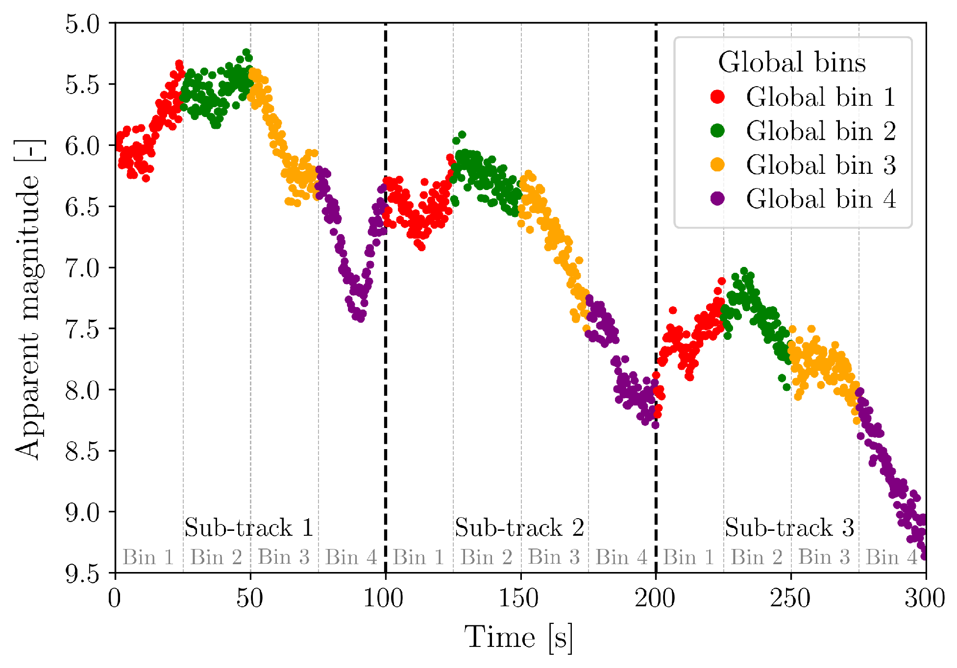
Afterwards, each sub-track is further divided into bins. The number of bins is the same for all sub-tracks, and it has been determined experimentally that partitioning each apparent rotation into 20 bins—each corresponding to a 18-deg rotation change—provides sufficient resolution to solve the light curve inversion problem accurately. The final step involves creating the measurement subsets, or global bins, by aggregating data from the corresponding bins across all sub-tracks. Measurements from the first bin of each sub-track are combined, followed by those from the second bin, and so forth.
The result of this pre-processing step is a set of global bins containing measurements taken at similar time points within a rotation period—meaning that roughly the same parts of the space object are observed—but at different elevation angles. Figure 2 illustrates the procedure using a portion of a light curve with an average apparent rotation period of approximately 100 s, divided into three sub-tracks and four bins. These numbers are provided for illustrative purposes only.

2.3.2. Global Estimation Method

Once the observed light curves have been pre-processed to generate the observation subsets, the iterative estimation method is initiated. The optical and atmospheric parameters, as well as the inertial spin period, are static. In contrast, the orientation parameters—namely, the orientation of the body-fixed reference frame with respect to the inertial reference frame, and the orientation of the spin axis relative to the body-fixed frame—change over time. Nevertheless, they are estimated at a specific time without requiring prior knowledge, in a manner conceptually analogous to Initial Orbit Determination (IOD) [53], where an unknown orbit is estimated from sensor measurements (e.g., range and range rate) at a given time, typically corresponding to the most recent observation.
Before describing the individual techniques and their integration within the overall estimation algorithm, it is first useful to introduce the foundations of the AISwarm-LS method. The AISwarm-LS method relies on statistical inference to estimate the unknown parameters from a probability distribution conditioned on the observed light curves. Let us define a d x dimensional vector of unknown static real parameters x X R d x that is assumed to follow a probability density function (pdf) defined as [54]:
π ˜ ( x ) = π ( x ) Z , Z = X π ( x ) d x
where π ( x ) is a non-normalised, non-negative pdf, and Z is a finite normalising constant. The challenge of the light curve inversion problem lies in the fact that the true pdf of the orientation parameters is not known a priori.
This is precisely where Importance Sampling methods [54] prove useful, providing an efficient means of estimating unknown parameters of a target probability distribution by drawing samples from a different, more tractable distribution. Let q ( x ) denote the so-called proposal or importance density, a pdf with heavier tails than the target distribution from which N independent samples { x i } i = 1 N can be easily drawn. A corresponding weighting function can then be defined to quantify the contribution of each sample drawn from q ( x ) in approximating the target distribution π ( x ) [54]:
w ( x ) = π ( x ) q ( x )
Consequently, the target probability distribution can be approximated by a weighted sum over the generated samples, as follows [54]:
π ˜ N ( x ) i = 1 N w ¯ ( x i ) δ ( x x i ) , x i q ( x )
where w ¯ ( x i ) are the normalised weights of the samples, calculated as [54]:
w ¯ ( x i ) = w ( x i ) i = 1 N w ( x i ) , x i q ( x )
Moreover, as the objective of the light curve inversion problem is to estimate the unknown parameters from the observed light curves, it can be formulated as a Bayesian inference problem. Bayes’ theorem is expressed mathematically as [54]:
π ˜ ( x ) = p ( x | z ) = 𝓁 ( z | x ) p 0 ( x ) Z ( z ) 𝓁 ( z | x ) p 0 ( x ) = π ( x )
where p ( x | z ) is the posterior pdf linked to the observed data z , 𝓁 ( z | x ) is the likelihood function, p 0 ( x ) is the prior pdf, and Z ( z ) is the model evidence or partition function. Since Z ( z ) is generally unknown and difficult to obtain, it is treated as a normalising constant Z for the non-normalised target pdf π ( x ) .
The weighting function can be incorporated into the Bayesian inference framework by substituting Equation (16) into Equation (13). This expression simplifies further if the importance density is chosen as the prior density at each iteration of the AISwarm-LS method, that is, q ( x ) = p 0 ( x ) :
w ( x ) = π ( x ) q ( x ) = 𝓁 ( z | x ) p 0 ( x ) q ( x ) = 𝓁 ( z | x )
The decision to process measurements using a batch strategy, as described in Section 2.3.1, requires a metric that quantifies the deviation between real and simulated measurements from multiple sensors with different noise levels. For this purpose, the Weighted Root Mean Square Error (WRMSE) is used and is computed for a given particle as [55]:
WRMSE = 1 M j = 1 M y j z j σ s , j 2
where z j is a real photometric observation, y j is the simulated measurement obtained for a particle state x i at the time of z j , M is the number of measurements selected in a given iteration, and σ s , j is the standard deviation of the corresponding sensor’s noise. The computation of each particle’s WRMSE requires propagating its attitude state to the times of the selected measurements using the kinematic model described in Section 2.1. Simulated measurements are then generated based on the observation model explained in Section 2.2. These calculations are performed in parallel to improve the computational efficiency.
The weight associated with each particle plays a crucial role in the Systematic Resampling and Clustering steps of the AISwarm-LS method. These weights are computed by mapping the particle’s WRMSE to a probability using a softmax function [56]:
w ¯ ( x i ) = 𝓁 { z j } j = 1 M | x i = exp WRMSE i 2 1 / T i = 1 N exp WRMSE i 2 1 / T
where the likelihood function represents the probability of observing the selected set of photometric measurements conditioned on a specific particle state.
A temperature parameter T is incorporated into the particle weight formulation in Equation (19) to implement Simulated Annealing [57,58]. This strategy aims to reduce the risk of premature convergence to local optima, particularly when Systematic Resampling is applied during the early stages of the AISwarm-LS method. The rationale for this approach arises from the relative nature of particle-based estimation methods, which assess each particle’s quality in comparison with others. Such relative evaluation can be problematic when multiple strong local optima are present, as in the current application. In addition to the inherent measurement ambiguities of the light curve inversion problem, the difficulty is compounded by the fact that the optical properties and the AOD are also estimated in the process for each candidate attitude state using a reduced subset of measurements, as explained in Section 2.3.4.
Simulated Annealing is therefore applied during the initial iterations of the light curve inversion method. Specifically, the temperature parameter decreases linearly from 5 to 1 over the first five iterations following the completion of the Adaptive Particle Allocation process. This strategy is particularly important when no prior knowledge of the object’s attitude exists and the method is initialised with a uniform particle distribution, as it flattens the weight distribution in the early stages, promoting broader exploration of the search space guided by the Particle Swarm Optimisation algorithm. As the temperature approaches unity, the weighting sharpens, allowing particles with lower WRMSE to dominate the distribution. Consequently, Systematic Resampling replicates the best-performing particles more aggressively, concentrating them in the most promising regions of the solution space for local exploration and refinement in subsequent iterations.
Returning to the operational details of the AISwarm-LS method, the initial proposal density is generated solely with respect to the orientation parameters, since the inertial spin period and the optical and atmospheric parameters are estimated implicitly using more computationally efficient techniques. The initial proposal density is typically chosen as a uniform distribution over the entire solution space, reflecting the usual lack of prior knowledge about the space object’s attitude. If a more accurate initial estimate is available, the proposal density can instead be initialised as a Gaussian distribution centred on that estimate, which helps accelerate convergence. The particle initialisation process respects the valid domain of each orientation parameter. Subsequently, the proposal distribution is updated at each iteration to more accurately approximate the target distribution, employing the adaptive strategy first introduced in [33] to address the challenges of the light curve inversion problem, which is also discussed in detail below.
As mentioned earlier, a group of measurements is selected to update the particle quality metrics at each iteration of the AISwarm-LS method. This selection involves randomly choosing one measurement from each global bin, ensuring that the selected measurements are spaced by at least the duration of a sub-track, corresponding to the initial estimate of the apparent rotation period. This strategy guarantees that the measurements collectively capture a full rotation of the object while including observations taken at different elevation angles. The adaptive process then proceeds through several steps that integrate different estimation and optimisation techniques. Initially, an Adaptive Particle Allocation strategy is applied during the early iterations to ensure the identification of all promising candidate solutions. In subsequent iterations, the combined use of Systematic Resampling and Particle Swarm Optimisation (PSO) enables thorough exploration of high-probability regions and accelerates convergence towards the most promising candidate solutions, while avoiding the computational cost associated with the explicit computation of the proposal distribution. A detailed description of these techniques is provided below, together with the Cluster Analysis used to assess convergence and determine the most probable solution.
(a)
Adaptive Particle Allocation
The adaptive allocation of particles is performed during the first two iterations of the AISwarm-LS method to refine the initial proposal distribution. The number of iterations for this technique was determined experimentally by analysing different test cases. This step is especially important when a uniform distribution is used as the initial proposal density. The primary goal is to ensure a robust exploration of the solution space, enabling the detection of all plausible candidate solutions. This approach also improves the estimation accuracy and the convergence performance in subsequent iterations.
The adaptive allocation process consists of relocating particles from low-probability regions to areas of the solution space with higher probability. Specifically, particles with a WRMSE in the upper tertile of the WRMSE distribution are repositioned near the best-performing particles. The new positions are determined using the sampling step of the initial proposal distribution, ensuring that the relocated particles occupy intermediate locations between the top-performing ones.
(b)
Systematic Resampling
Resampling is a statistical technique in which samples are repeatedly drawn from a dataset to improve the accuracy of probability distribution estimates. It helps mitigate the particle degeneracy problem [59], which arises when only a small subset of particles carries significant weight while the majority contribute little to the overall estimate. In such situations, computational resources are wasted on particles that provide no valuable information. An estimate of the effective sample size, which quantifies this issue, is [60]:
N ^ e f f = 1 i = 1 N w ¯ i 2
where w ¯ i is the normalised weight of each particle and N is the total number of particles.
The resampling strategy adopted in this work selects new particles with replacement from the weighted particle set, keeping the total number of particles constant. Particles with higher weights are more likely to be selected multiple times, whereas those with lower weights tend to be discarded. Among the different resampling algorithms available in the literature, Systematic Resampling [61] is chosen for the AISwarm-LS estimation method because it is simple to implement, takes O ( N ) time, and minimises the Monte Carlo variation [60].
The Systematic Resampling and Particle Swarm Optimisation (PSO) steps are applied within the AISwarm-LS method to update the particle states for the next iteration whenever the convergence criteria from the Cluster Analysis is not satisfied. The application of Systematic Resampling not only reduces the computational cost of updating low-weight particles, but also improves the convergence of the method when used in conjunction with PSO. It is particularly effective at removing particles from regions that initially appeared to have high probability but become less relevant as the estimation process progresses. This reallocation typically occurs as new photometric measurements are incorporated, and the estimation of the true optimal solution is progressively refined. Systematic Resampling is executed prior to PSO if the effective sample size falls below 25% of the total number of particles, a reasonable threshold also employed in particle filters [62].
(c)
Particle Swarm Optimisation
Particle Swarm Optimisation (PSO) [63] is a population-based global optimisation algorithm that mimics the social behaviour of birds flocking or fish schooling to find optimal solutions in a search space. PSO has been successfully applied in a wide range of application domains [64]. In this work, PSO is adopted not only for its performance but also for its simplicity—its particle update mechanism requires tuning only a few parameters—and for its adaptability, which makes it well suited for integration into the AISwarm-LS method.
In PSO, a group of candidate solutions (particles) move through the search space according to their momentum, which adjusts the trajectory of the particles and accelerates their convergence towards optimal solutions. The momentum of the particles is updated iteratively based on both their own experience and that of the neighbouring particles (the swarm). In this case, a particle’s position vector corresponds to the set of orientation parameters at the reference time to be estimated. Let the j-th component of the i-th particle’s position and velocity vectors at iteration k be denoted as x i , j k and v i , j k , respectively. Each scalar orientation parameter and its associated velocity are then updated according to the following equations [65]:
v i , j k = w v i , j k 1 + c 1 r 1 ( x i , j p b e s t x i , j k ) + c 2 r 2 ( x j g b e s t x i , j k ) x i , j k = x i , j k 1 + v i , j k
where w is the inertia weight factor, c 1 is the cognitive coefficient, x i , j p b e s t is the j-th component of the best state found by the i-th particle (personal best), c 2 is the social coefficient, x j g b e s t is the j-th component of the best state found by any particle in the swarm (global best), and r 1 and r 2 are random numbers drawn from U ( 0 , 1 ) .
In the proposed AISwarm-LS method, PSO is used to assist in the implicit estimation of the target probability distribution, avoiding the computational cost of explicitly computing it at each iteration. In addition, PSO provides a more efficient alternative to traditional techniques commonly employed in particle filters to preserve particle diversity, such as the injection of artificial noise, enabling faster convergence to the correct solutions. PSO is applied in combination with Systematic Resampling once the Adaptive Particle Allocation phase is completed, and it continues to update the proposal distribution in subsequent iterations until the convergence criteria are satisfied.
The PSO parameters are chosen to prioritise local exploration during the early iterations of the AISwarm-LS method and, as the process progresses, to promote exploitation by accelerating the convergence of particles towards globally optimal states [66]. This behaviour is achieved by linearly decreasing the inertia weight and the cognitive coefficient, while simultaneously increasing the social coefficient. The parameter values, determined experimentally, are set to w m i n = 0.2 , w m a x = 0.4 , c 1 , m i n = c 2 , m i n = 0.5 , c 1 , m a x = c 2 , m a x = 2.5 . The linear variation of these parameters is applied during the same iterations in which Simulated Annealing is active, that is, until K = 5 . For all subsequent PSO executions, the parameter values reached at iteration K are retained.
In the first execution of PSO, directly applying Equation (21) would make the particle velocity depend solely on the global best state, since particles have no prior velocity and their personal best state coincides with their current state. In the AISwarm-LS framework, this can be problematic because each particle’s WRMSE is computed using the optical properties and AOD that minimise the residuals with respect to the measurements selected in that iteration, which may lead to convergence to local optima or overfitting. To mitigate this and promote broader exploration of the solution space in the early iterations, the particle velocity is initialised using the following equation, which combines attraction towards the global best state with an exploratory component:
v i , j k = 1 = c 2 , m i n r 2 ( x j g b e s t x i , j k = 1 ) + r 3 Δ i , j
where c 2 , m i n = 0.5 , r 2 U ( 0 , 1 ) , r 3 U ( 1 , 1 ) , and Δ i , j is the exploratory step, computed as follows:
Δ i , j = Δ j , m i n + η i ( Δ j , m a x Δ j , m i n )
η i = WRMSE i * WRMSE m i n WRMSE Q 3 WRMSE m i n
Here, Δ j , m a x is half the sampling step of the initial uniform proposal distribution for the j-th state parameter, and Δ j , m i n = Δ j , m a x / 2 . The parameter η i [ 0 , 1 ] represents a particle performance score. WRMSE m i n is the minimum WRMSE across the swarm, while WRMSE Q 3 denotes the third quartile of the WRMSE distribution. The value WRMSE * = min WRMSE i , WRMSE Q 3 clamps the actual WRMSE of the i-th particle, WRMSE i , to the third quartile value to mitigate the influence of outliers.
Finally, it is important to bear in mind that the target probability distribution is likely to be multimodal. Therefore, PSO must maintain a set of global best states, which is updated at each iteration based on two criteria that must be satisfied simultaneously:
  • Selected particles must have a WRMSE within the first tertile of the current iteration’s WRMSE distribution. Replicated particles resulting from the resampling step, if any, are considered only once. Global best states from the previous iteration that meet this WRMSE threshold are also retained.
  • Only the particle with the lowest WRMSE within a defined neighbourhood is selected. Neighbourhoods are defined under the assumption that distinct attitude solutions cannot exist within an angular separation of 30 deg. Two particles are considered to belong to the same neighbourhood if the angular distance between their respective attitude states is lower than this threshold.
At each iteration of PSO, the velocity of each particle is updated considering its nearest global best state, which is identified using the Manhattan distance [67] calculated across all orientation parameters and taking into account the periodicity of some of them.
(d)
Cluster Analysis
Clustering is a technique used to group similar data points based on shared characteristics. The proposed light curve inversion method uses Density-Based Spatial Clustering of Applications with Noise (DBSCAN) [68] to identify the modes of the target probability distribution, assess the convergence of the estimation process, and compute the most likely solution within each cluster along with its associated standard deviation.
DBSCAN identifies clusters according to the density of data points. Unlike partition-based methods like K-Means, DBSCAN does not require the number of clusters to be specified in advance. Instead, it operates based on two key parameters:
  • The neighbourhood radius, which defines the maximum distance within which a point is considered a neighbour of another point.
  • The minimum number of points required to form a cluster.
The DBSCAN implementation from the Hipparchus library [69] is used in this work. However, due to the presence of different types of unknown parameters—orientation angles, reflection coefficients and AOD—a customised distance metric is defined as the average Manhattan distance [67] computed across all parameters. This metric is normalised using half the sampling step of the initial proposal distribution for the orientation parameters and half the parameter range for the optical and atmospheric parameters. The inertial spin period is not considered in the clustering process, as it is a direct consequence of the orientation parameters. The threshold values used to identify particle clusters have been determined empirically by analysing different test cases. Specifically, the minimum cluster size is set to 10% of the total number of particles, and the neighbourhood radius is set to 0.1 in terms of the average normalised Manhattan distance.
Once a cluster is identified, the posterior expected state x ^ and its associated covariance matrix Σ can be computed as [70]:
x ^ = i = 1 N w ¯ i x i
Σ = i = 1 N w ¯ i x i x ^ x i x ^ T
The Cluster Analysis is performed from the seventh iteration onwards, after the Simulated Annealing process concludes, since it is computationally intensive. This delay allows the particles a few iterations to move towards high-probability regions of the solution space and was determined experimentally through the analysis of different test cases. Two criteria are defined to assess the convergence of the AISwarm-LS light curve inversion method, ensuring accurate and robust estimation of the unknown parameters:
  • Global criterion: at least 80% of the particles must be assigned to a cluster.
  • Local criterion: the WRMSE associated with the state estimate of each cluster must be below 1.1, and the relative change in WRMSE between consecutive iterations must be less than 5%.
The local criterion is evaluated after refining the weighted average state through a two-step optimisation process. This refinement is necessary to obtain a stable WRMSE metric for assessing convergence, since small changes in any of the attitude, optical or atmospheric parameters can produce significant variations in the resulting WRMSE.
In the first refinement step, the estimates of the optical and atmospheric parameters are improved using the Least Squares Method (LSM) described in Section 2.3.4, applied to an extended set of photometric measurements sampled from the observed light curve at a configurable time interval. This initial optimisation is necessary because, in each iteration of the AISwarm-LS method, only 20 measurements are employed to update the particle quality metrics and maintain computational efficiency. As a result, the estimation accuracy may be insufficient, particularly if some material components are not observed at the time of the selected measurements or if their contribution is dominated by other materials observed simultaneously.
In the second refinement step, the weighted average attitude state from the cluster, together with the refined estimates of the optical and atmospheric parameters obtained in the first refinement step, are jointly refined using Powell’s Bound Optimisation BY Quadratic Approximation (BOBYQA) algorithm [71]. The objective is to minimise the WRMSE with respect to the extended set of observed measurements. In this work, the BOBYQA implementation provided by the Hipparchus library [72] is employed.
Powell’s BOBYQA is a derivative-free optimisation algorithm designed for solving non-linear, bound-constrained problems. Analytic partial derivatives of the residuals with respect to the attitude parameters are unavailable, and numerical derivatives are often unstable and expensive to compute. Therefore, BOBYQA’s reliance solely on function evaluations to iteratively construct and update a quadratic approximation of the objective function makes it especially well-suited for this application. The number of interpolation points used to construct the quadratic model is 2 d x + 1 [72], where d x is the dimension of the vector of unknown parameters. In order to ensure sufficient margin to optimise the solution, the search of all parameters is constrained within the ± 3 σ range, where σ is the weighted standard deviation for each parameter.
If convergence is not achieved, the proposal distribution is updated for the next iteration through the combined use of Systematic Resampling and PSO, as described above. The refined estimate of each cluster is incorporated into the particle set by replacing the particles with the highest WRMSE values.

2.3.3. Inertial Spin Period Estimation

Once a set of orientation parameters is defined according to the methodology described in Section 2.3.2, the inertial spin period remains the only parameter required to fully characterise the object’s attitude. Although this parameter could, in principle, be estimated jointly with the orientation parameters, doing so would necessitate sampling in a higher dimensional space. Since the AISwarm-LS method is sensitive to the curse of dimensionality, reducing the dimensionality even by a single parameter results in a significant improvement in computational efficiency, which is particularly important in operational scenarios.
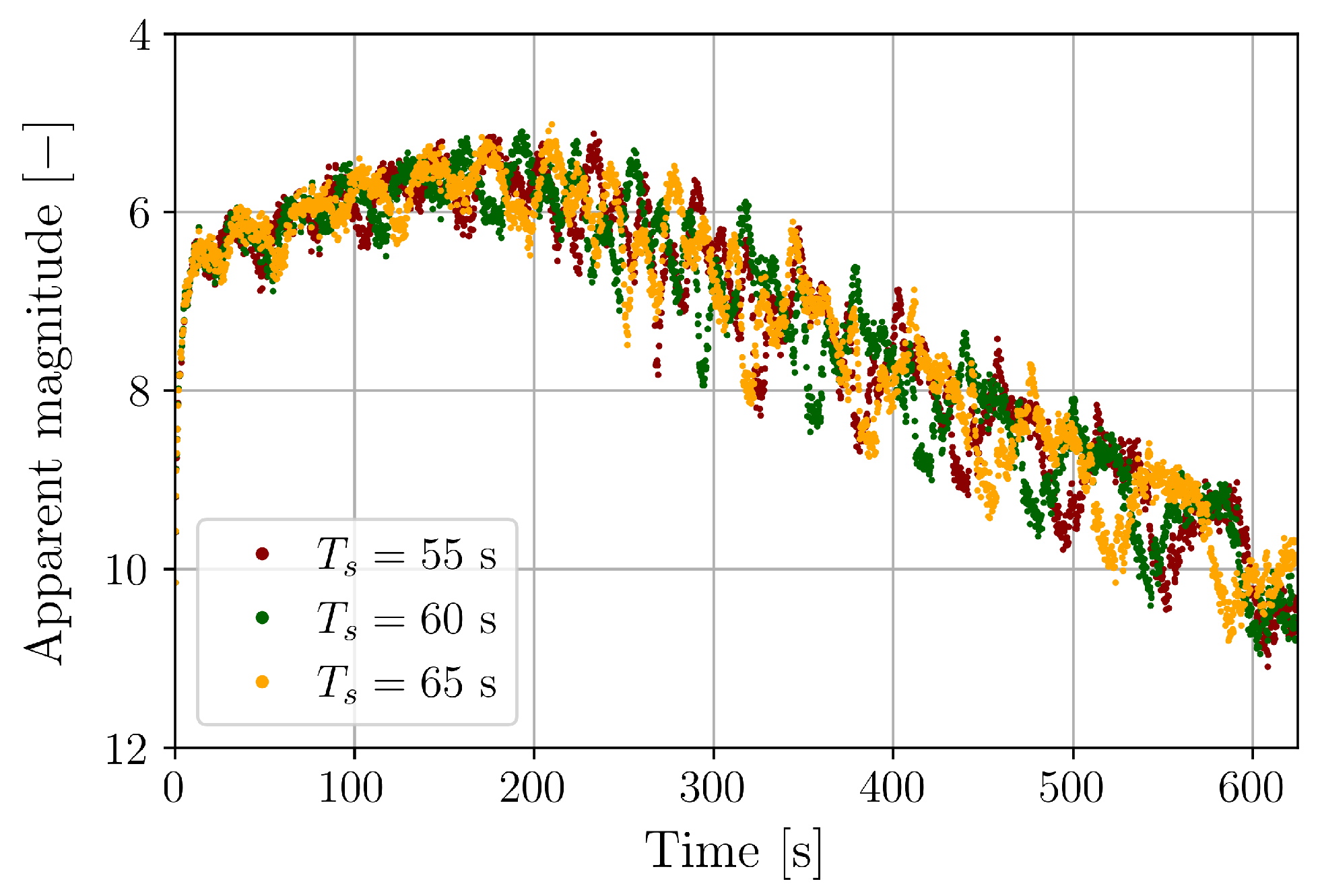
This dimensionality reduction is possible because, for a given set of orientation parameters, the inertial spin period can be reliably inferred from the observed light curve. The influence of the inertial spin period on the light curve is illustrated in Figure 3 for the satellite model presented in Section 3. Since the spin period is independent of the vertical shifts caused by the reflection coefficients or atmospheric attenuation, it is estimated individually for each particle at the start of every AISwarm-LS iteration, prior to the estimation of the material and atmospheric parameters.
The estimation of the inertial spin period is based on the relationship between the magnitude of the inertial angular velocity ω i n e r t i a l , the apparent angular velocity observed from the sensor location ω a p p a r e n t , and the projection of the topocentric orbital angular velocity ω o r b i t onto the direction of the inertial spin axis u ^ ω i n e r t i a l :
ω i n e r t i a l = ω a p p a r e n t ω o r b i t · u ^ ω i n e r t i a l
where ω o r b i t is computed from the position and velocity vectors of the space object in the topocentric reference frame centred at the sensor location.
The apparent angular velocity can be estimated from the observed light curve using the Lomb–Scargle periodogram [52]. In contrast, the topocentric orbital angular velocity can be computed directly, as the topocentric position and velocity of the space object are known over the observation interval. However, it is important to note that both the apparent angular velocity and the orbital angular velocity as observed from the ground station change over time. In fact, the result of the Lomb–Scargle periodogram can be interpreted as an average of the dominant frequencies within the selected signal range. Since the Lomb–Scargle periodogram requires a time series covering at least two full apparent rotations to reliably determine the dominant frequency of the photometric signal, a time interval spanning 2.5 times the initial estimate of the apparent rotation period—derived from the complete light curve—is selected. To mitigate the impact of variations in orbital angular velocity relative to the topocentric frame, the interval is chosen to minimise changes in observation elevation, which typically occurs near the zenith.
The apparent rotation period and the average topocentric orbital angular velocity are estimated once, prior to the iterative steps of the AISwarm-LS method. At each iteration, the inertial spin period for each particle is then computed using Equation (27), with the direction of the inertial spin axis derived from the particle’s orientation parameters.

2.3.4. Optical Properties and AOD Estimation

Important parameters in the light curve inversion problem, due to their strong coupling with the attitude state, are the optical properties of the space object’s surfaces and the atmospheric conditions at the sensor location. The diversity of aerospace materials, combined with their degradation after prolonged exposure to the space environment, makes their estimation at the time of observation necessary for reliable characterisation. With respect to the atmospheric sources of light extinction, aerosol attenuation is governed by the Aerosol Optical Depth (AOD) at the sensor location, which can vary significantly with weather conditions. Consequently, the AOD is incorporated into the estimation process to eliminate the need for on-site measurements at the time of observation.
Regarding the optical properties of materials, this work focuses on estimating their diffuse reflection coefficients, since the specular contribution arises only under specific relative geometries between the Sun, the satellite, and the sensor. This strategy is supported by previous studies. A global albedo of 0.175 is recommended in [73] for debris objects, although the later work in [74] reported variability in this reference value, ranging from 0.12 to 0.275. Moreover, the primary factor influencing the reflectance spectra of three-axis stabilised GEO satellites is the presence of Multi-Layer Insulation (MLI) on the platform surface [75]. Different MLI materials are analysed in [76], with diffuse reflectance reported to range from 0.05 to 0.25. However, the wide range of aerospace materials used in satellite components leads to greater variability, with some materials exhibiting substantially higher values than MLI, such as white paint [77,78] or certain aluminium alloys [77,79,80]. In contrast, solar arrays can be modelled as purely specular reflectors, consistent with previous studies [77,81], which report an albedo of approximately 0.1 with minimal dispersion.
In a previous work by the authors [82], the attitude of an uncontrolled space object was accurately estimated using a global diffuse reflection coefficient, which accounted for the contributions of the different materials. However, this approach has a significant limitation because a set of attitude parameters differing from the true values, when combined with a uniform material for all main body surfaces, could produce a photometric signature that matches the observed one. Moreover, the estimation of the global diffuse coefficient is insufficient for accurate modelling of the solar radiation pressure. These limitations, together with the wide variety of aerospace materials and the fact that exposure to the space environment can alter their optical properties unpredictably, led to abandoning that approach in the present work. In the current AISwarm-LS method, a diffuse reflection coefficient is estimated for each material composing the main body of the space object.
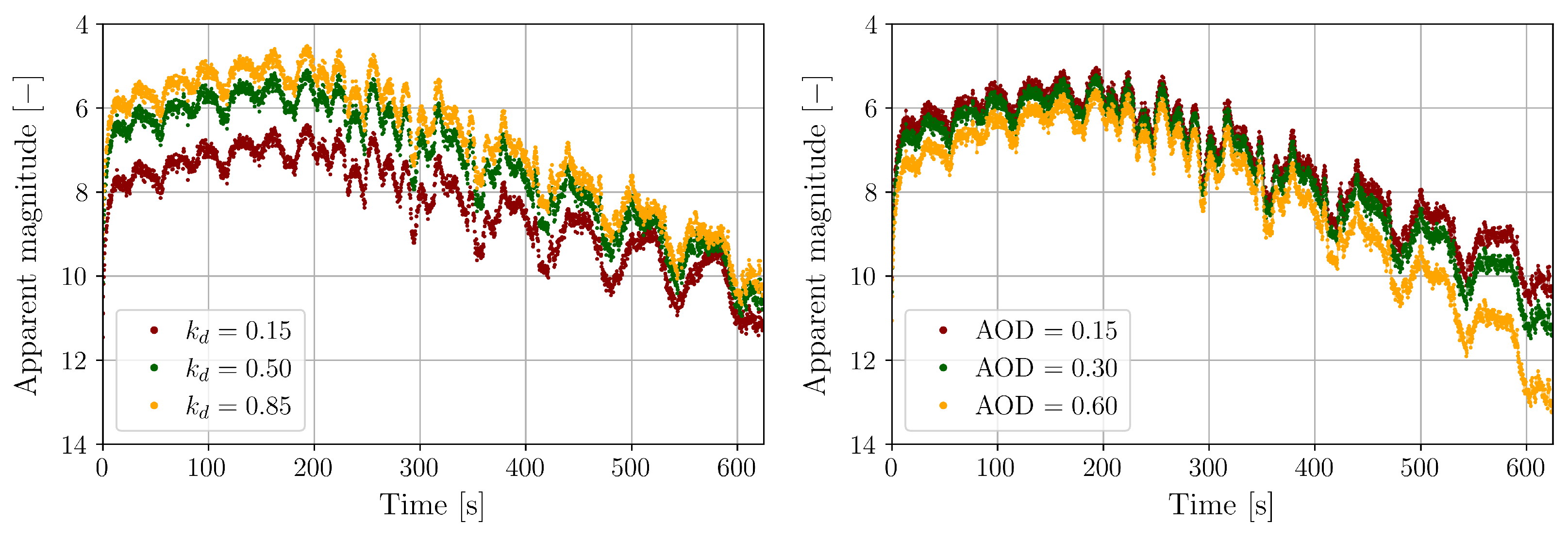
The influence of the diffuse reflection coefficient and the AOD on the resulting light curve is shown in Figure 4. The satellite model presented in Section 3 is used with uniform material properties for all the surfaces, and only the diffuse reflection coefficient and the AOD are varied in their respective plots. The effect of these parameters becomes more evident when the light curve is analysed in its entirety rather than through individual measurements, which further supports the batch processing strategy of photometric measurements. For space objects with uniform material properties, such as a rocket fairing, the diffuse optical properties affect all measurements similarly, producing a vertical shift. However, for objects composed of different materials, the problem becomes more complex, as each measurement is affected differently depending on the surface or combination of surfaces observed at that moment. Regarding the attenuation of light due to aerosols, the AOD produces a consistent shift in magnitude, but this effect is modulated by the air mass between the space object and the sensor. Consequently, the attenuation is stronger at lower elevation angles, typically occurring at the beginning and end of the observation interval.
The estimation of the diffuse optical properties of the different materials composing the surfaces of the space object, as well as the AOD at the different sensor locations, is performed using a Least Squares Method (LSM). As indicated in Figure 1, this estimation is carried out for each particle at every iteration of the AISwarm-LS method. Unlike the approach introduced in [82], the LSM avoids increasing the dimensionality of the state associated with the particle-based methods, improving the computational efficiency. Once the diffuse reflection coefficients and the AOD have been estimated, the simulated measurements can be computed at the times corresponding to the selected observations, enabling the particle quality metrics to be obtained. The LSM is adopted because the observation model defined in Equations (3)–(11) can be expressed analytically in terms of the k d , Γ and AOD parameters:
m s i m = 2.5 log Γ C Γ k d , Γ + I o , a r r a y I r e f + 2.5 m a i r ln 10 A O D + T R a y + T O 3
C Γ = I i 2 π r 2 I r e f γ Γ A γ ( l · n ) γ ( v · n ) γ ( l · n + v · n ) γ
where the subscript Γ refers to surface components of the object that share the same diffuse reflection coefficient k d , Γ , while the subscript γ denotes the facets into which each surface Γ is divided to compute its contribution to the reflected light. The term I o , a r r a y represents the observed irradiance from the solar arrays of the space object, if present. In this work, the worst-case scenario, in which only photometric measurements from a single sensor are available, is considered. Nevertheless, the formulation can be readily extended to incorporate measurements from multiple sensors or different observation windows by estimating the AOD at each sensor location and for each time window. Furthermore, as previously discussed, only the specular contribution of the incident irradiance from the solar arrays is considered (but not estimated), while the surfaces of the main body are modelled as purely diffuse reflectors.
The Levenberg–Marquardt (LM) algorithm [83,84], as implemented in the Hipparchus library [85], is employed to solve the non-linear least squares problem. This optimisation algorithm combines the fast local convergence of the Gauss–Newton method with the global stability of gradient descent. Its ability to exploit analytical Jacobians while maintaining robustness in the presence of non-linearities makes it particularly well-suited for this estimation problem. Moreover, the Levenberg–Marquardt algorithm performs unconstrained optimisation, preserving the advantages of such methods—most notably computational efficiency and algorithmic simplicity—while avoiding the additional overhead typically associated with constrained solvers. This benefit is especially important in the present work, as the algorithm is executed for every candidate particle at each iteration of the AISwarm-LS method.
Since the domains of the unknown parameters k d , Γ and AOD are constrained to the interval [ 0 , 1 ] , applying an unconstrained optimisation algorithm like Levenberg–Marquardt can be problematic. This issue is effectively addressed through a reparametrisation strategy, in which each constrained parameter is expressed as a smooth, differentiable function of an unconstrained variable. This ensures that the residuals and their Jacobians remain continuous, a property essential for reliable convergence in non-linear least squares solvers. The standard logistic function [86] is convenient for this purpose, as it maps the entire set of real numbers R onto the open interval ( 0 , 1 ) :
σ ( u ) = 1 1 + exp ( u )
Therefore, the Levenberg–Marquardt algorithm operates on the unconstrained variables, which are related to the constrained parameters through the transformations k d , Γ = σ ( u k d , Γ ) for the diffuse reflection coefficient of surface Γ , and A O D = σ ( u A O D ) for the Aerosol Optical Depth at the sensor location. With this reparametrisation strategy, the parameters are automatically confined to their physically meaningful domain, eliminating the need for additional constraint-handling techniques, such as penalty terms or post-iteration projections.
Moreover, the residual function ϵ used in solving the least-squares problem with the Levenberg–Marquardt algorithm is defined as the difference between the observed apparent magnitude m o b s and the simulated measurement m s i m given by Equation (28). This difference is normalised by the standard deviation of the sensor noise σ s , expressing the residual in units of measurement uncertainty, as shown in Equation (31). Such normalisation improves both the accuracy and robustness of the estimation, particularly when incorporating photometric measurements from different sensors.
ϵ = m o b s m s i m σ s
The partial derivatives of the residual with respect to the unconstrained parameters, which constitute the Jacobian matrix, are given by:
ϵ u k d , Γ = 2.5 C Γ k d , Γ 1 k d , Γ Γ C Γ k d , Γ + I o , a r r a y I r e f σ s ln 10
ϵ u A O D = 2.5 m a i r A O D 1 A O D σ s ln 10
Finally, it is worth noting that the previous LSM problem can be simplified if the optical properties of the surfaces do not need to be estimated, as Equation (28) is linear with respect to the AOD. In this case, the AOD can be estimated using an Ordinary Least Squares (OLS) method [87]. This simplified approach is also applicable for the simultaneous estimation of the diffuse reflection coefficient and the AOD, provided that all surfaces of the space object are made of the same material and there are no specular contributions from any component.

3. Results and Discussion

This section presents the results of the analysis performed to evaluate the performance of the proposed light curve inversion method. The objective is to estimate the attitude parameters and the optical reflective properties of an uncontrolled space object of known shape, together with the AOD at the sensor location. The study considers the worst-case scenario, in which only photometric measurements from a single sensor are available and no prior knowledge of the unknown parameters is assumed. This case study reflects realistic operational conditions, such as situations in which a satellite operator has lost control of a satellite and seeks to assess the feasibility of In-Orbit Servicing (IOS) or Active Debris Removal (ADR) operations, or scenarios in which accurate estimation of attitude and optical parameters is required to improve the reliability of other Space Surveillance and Tracking (SST) activities, including collision risk assessment or atmospheric re-entry predictions.
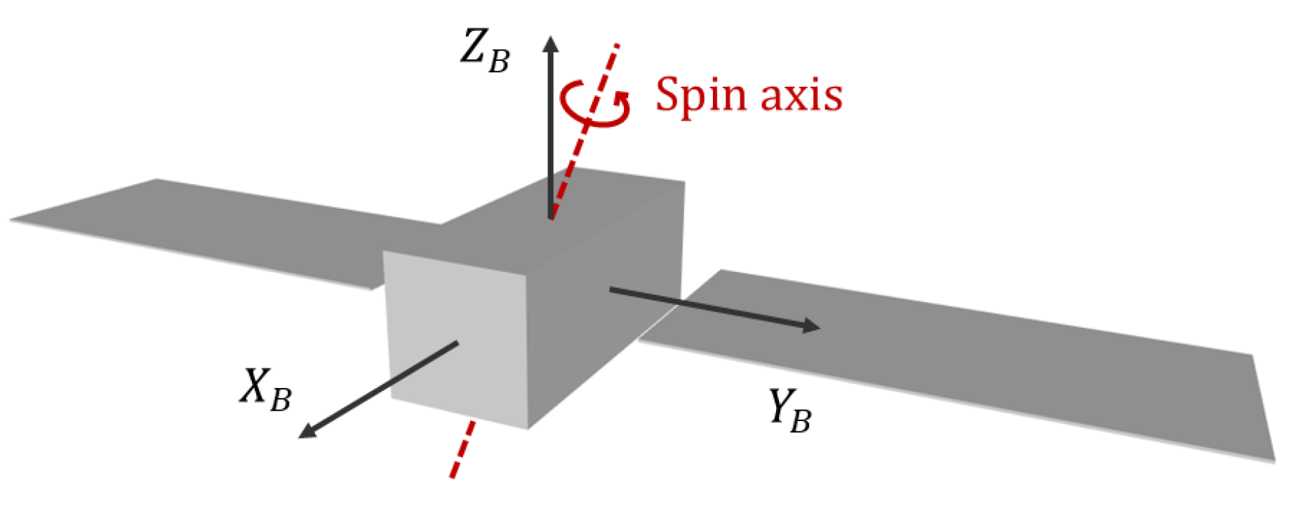
The satellite is in a circular orbit at an altitude of 1000 km, with an orbital inclination of 20 deg and a right ascension of the ascending node of 0 deg. The satellite model, shown in Figure 5, consists of a quadrangular prism platform with dimensions 2.5 × 1 × 1 m, and a solar array measuring 1.5 × 3.5 × 0.01 m, resulting in a total span of 9 m. The reference attitude at the time of the first observation and the reference optical and atmospheric parameters are provided in Table 1. As discussed in Section 2.3.4, the platform is assumed to be a purely diffuse reflector, while the solar arrays are modelled as purely specular reflectors with k s = 0.1 . All surfaces are assigned a roughness coefficient of n s = 0.1 .
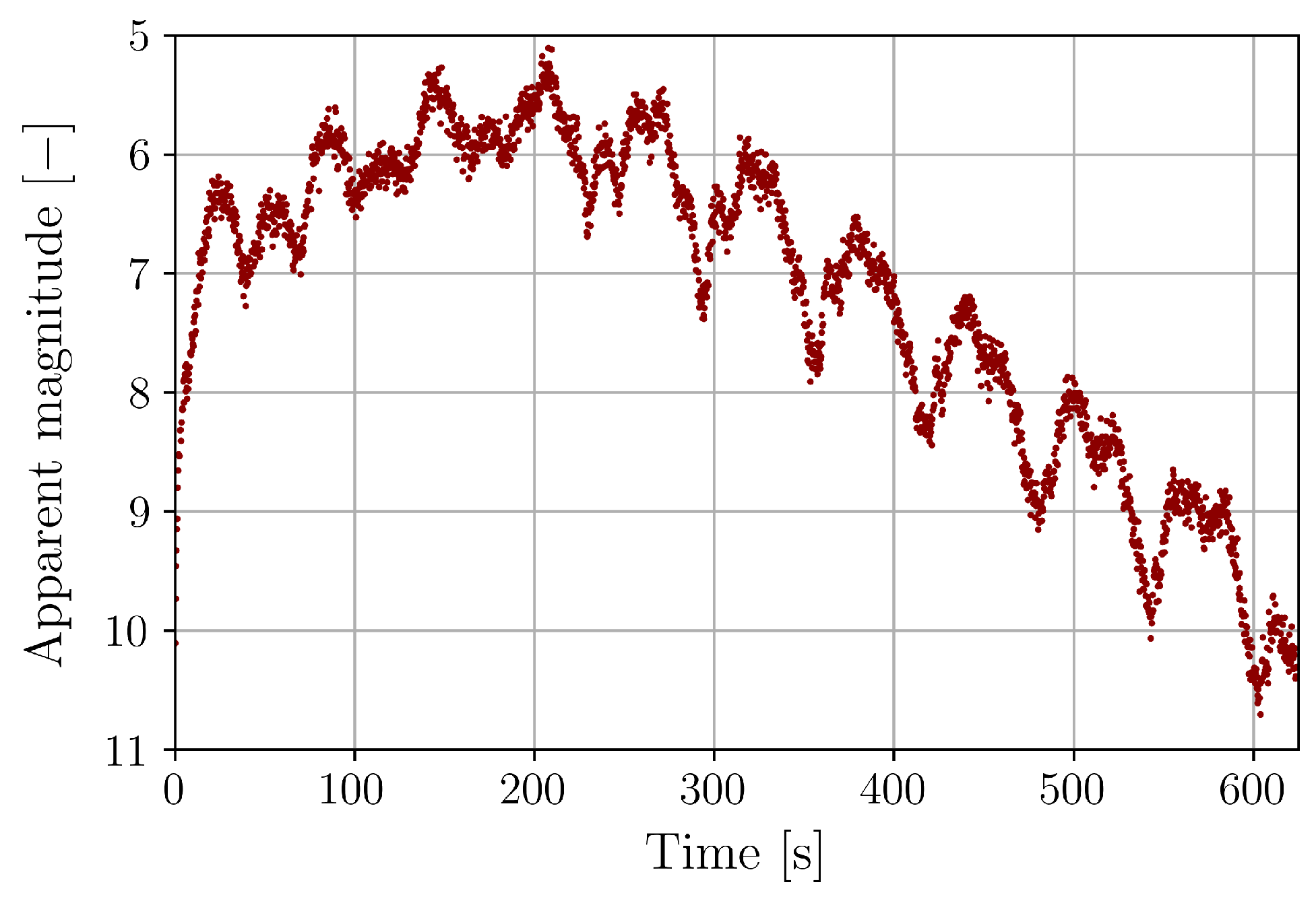
The satellite model, with the previous reference attitude, optical and atmospheric parameters, produces the light curve shown in Figure 6, as observed from a hypothetical sensor located at 5° N, 20° E, 1600 m above mean sea level (WGS84). The light curve is simulated with a sensor noise standard deviation of σ s = 0.1 in apparent magnitude.
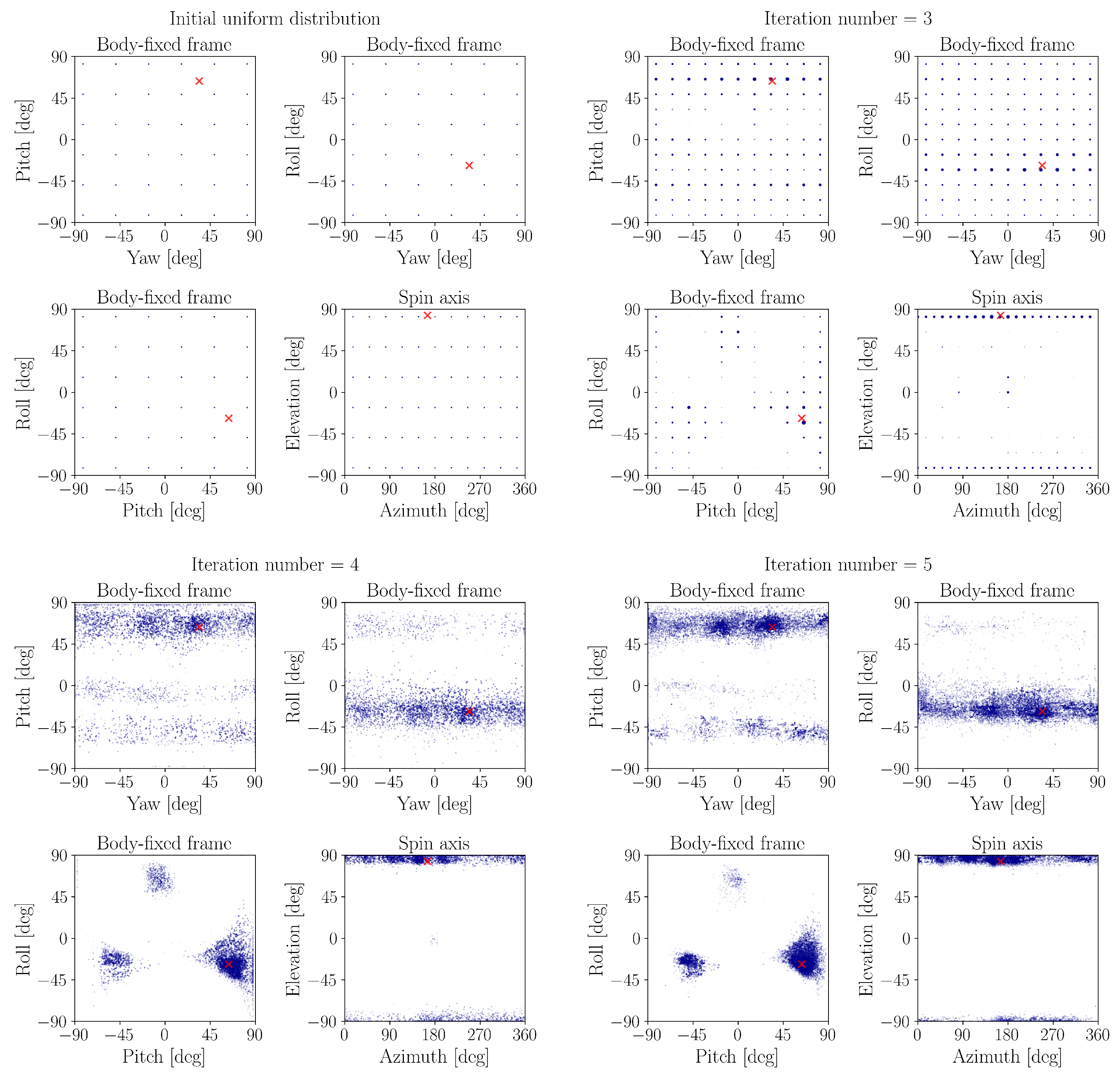
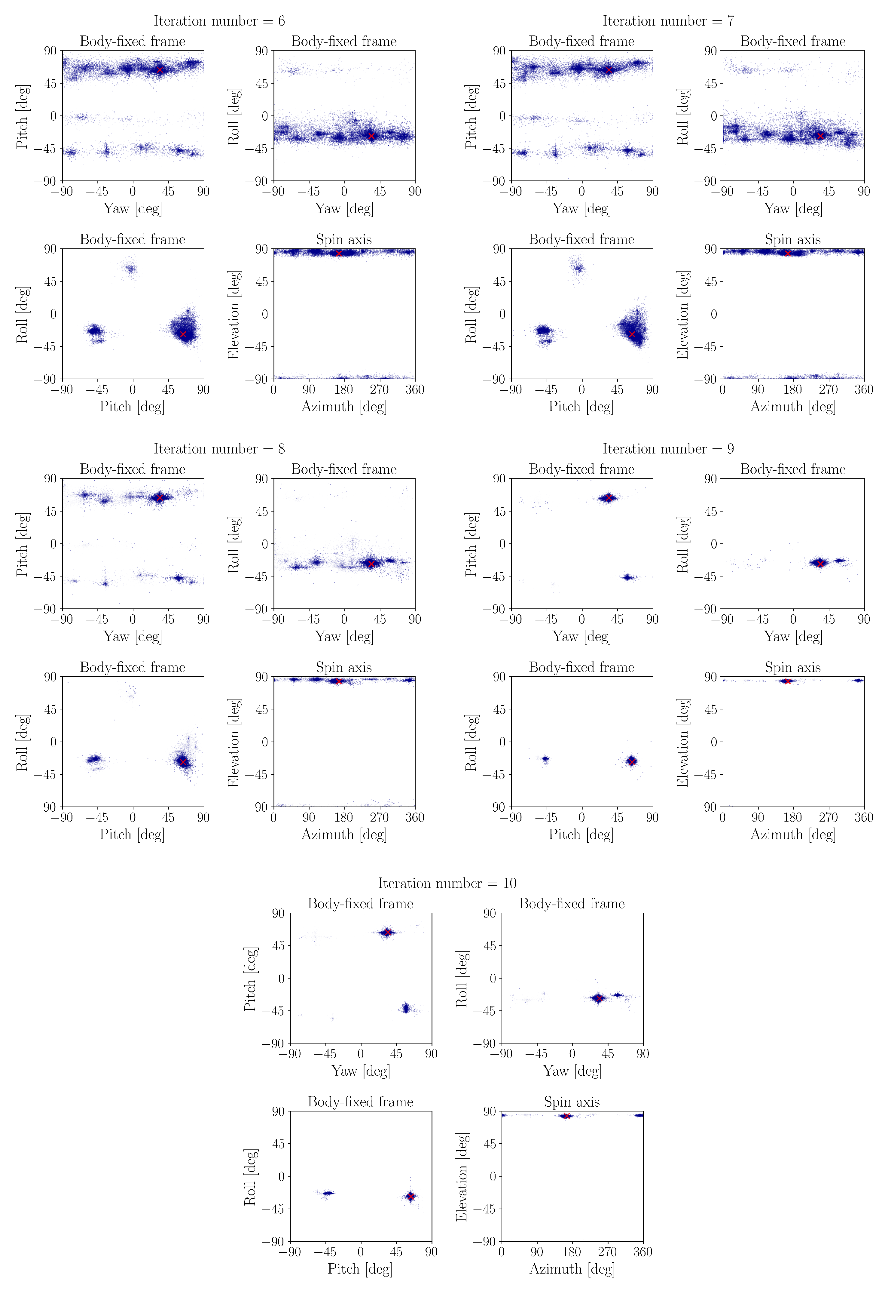
The execution of the AISwarm-LS method is illustrated in Figure 7, which shows the distribution of particles within the solution space of the orientation parameters across different iterations. The actual attitude state to be estimated is marked by a red cross. The process begins by pre-processing the reference light curve to create the global bins used for selecting measurements at each iteration. A uniform distribution of particles is then generated across the solution space, as no prior knowledge of the attitude is assumed. The solution space is constrained by the symmetric geometric and optical properties of the satellite model, so any solutions identified within the defined search domain will have corresponding symmetric attitude states. The sampling resolution was determined experimentally by analysing different test cases, and it was found that dividing the 360-deg range into 11 equally spaced intervals provides a sufficiently fine discretisation to solve the problem accurately. This configuration results in a total of 14,256 particles.
The first two iterations of the AISwarm-LS method are devoted to exploring the search space through the Adaptive Particle Allocation process, ensuring the identification of all high-probability regions. As shown in Figure 7, by the third iteration, high-probability regions begin to emerge. At this iteration, the particle velocities are computed considering both the global best states and an exploratory term, which enables further exploration of these regions. In subsequent iterations, particles progressively accelerate towards the most promising candidate solutions through the combined effects of Systematic Resampling and PSO. The linear evolution of the PSO parameters, together with the temperature schedule of the Simulated Annealing process, ensures that convergence occurs gradually, reducing the likelihood of becoming trapped in local optima. A cluster is identified for the first time at the ninth iteration, in which the absolute convergence criterion is already satisfied. Both the local and the absolute convergence criteria are satisfied at the tenth iteration, achieving a WRMSE of 1.008 and a relative change of 3.41% compared to the previous iteration.
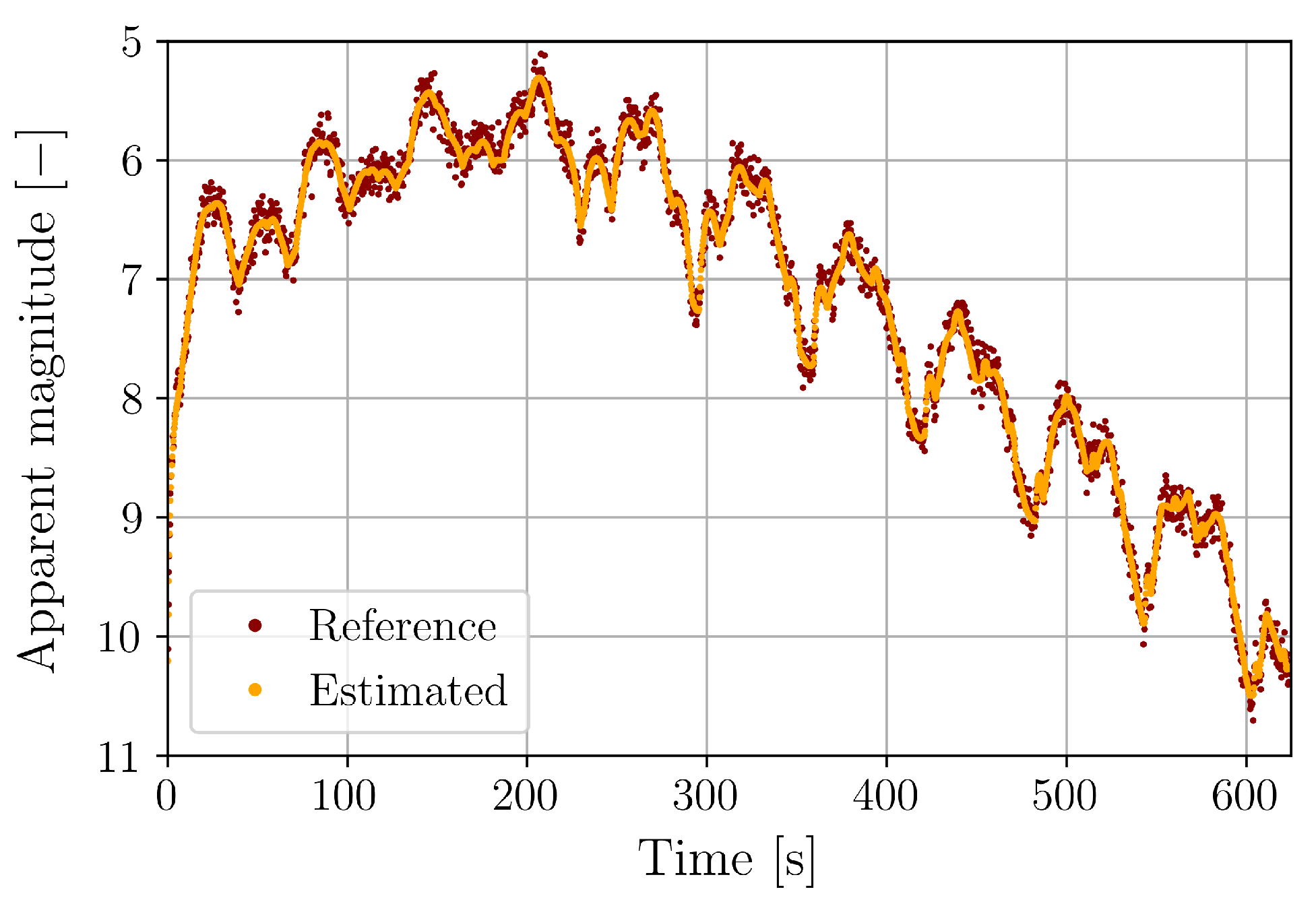
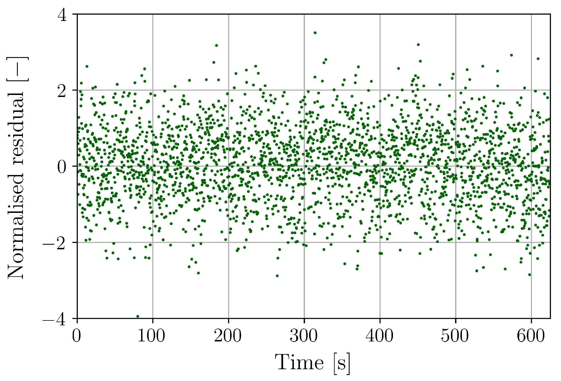
The numerical results obtained at the iteration in which convergence is achieved are presented in Table 2. The table reports the weighted average and standard deviation of the cluster, together with the final estimates of each parameter after the refinement step. For comparison, the reference parameters are also provided. As can be observed, the weighted state of the cluster already yields a relatively good approximation to the reference parameters. However, because small variations in any of these parameters produce substantial changes in the resulting WRMSE, a refinement procedure is necessary. This refinement is performed using the extended subset of measurements. Firstly, the analytical LSM with the Levenberg–Marquardt algorithm is applied to the material parameters. Then, the derivative-free LSM with the BOBYQA algorithm is applied to all the parameters. This two-stage process further reduces the WRMSE, enabling the convergence thresholds to be satisfied. Notably, the final WRMSE is very close to unity, indicating that the discrepancy between the estimated and reference light curves is comparable to the noise used to generate the reference photometric measurements. It is important to note that the weighted standard deviation of the cluster is not a reliable measure of the final parameter estimation error, as it is computed using only the reduced subset of measurements.
The light curve obtained using the final AISwarm-LS parameter estimates is shown in Figure 8, together with the reference light curve. To further evaluate the accuracy of the solution, the residuals between each simulated measurement and the corresponding reference values are computed and normalised by the standard deviation of the sensor noise. These normalised residuals are shown in Figure 9, where it can be seen that the majority of the measurements, specifically 95.43%, lie within the ± 2 normalised residual range. The results show that the light curve inversion method can accurately estimate the attitude, optical, and atmospheric parameters. The deviations from the reference parameters arise from the measurement noise. Moreover, the present test case is partially affected by the indetermination of the azimuth angle of the spin axis, as the elevation angle of the spin axis is 83.5 deg, which is relatively close to 90 deg, where the azimuth becomes fully undetermined. This effect leads to a greater dispersion of particles in the azimuth component.
Finally, the computational cost associated with each process of the AISwarm-LS light curve inversion method is provided in Table 3. The analysis of the test case was performed on a computer equipped with an Intel(R) Core(TM) i7-10610U CPU @ 1.80 GHz, using eight parallel threads, and an Intel(R) UHD Graphics GPU with 7.9 GB of memory. The reported results correspond to the average processing time per iteration for the 14,256 particles used in the test case. The total time represents the duration required to satisfy both the absolute and the relative convergence criteria.
As can be observed, the most computationally demanding step is the simulation of photometric measurements, followed by the clustering process. The number of measurements simulated depends on the number of different materials in the object model (four in this test case), but the process is fully parallelised, enabling significant computational improvements to be readily achieved through the use of additional CPU cores. By contrast, the DBSCAN algorithm is particularly affected by the curse of dimensionality because of its neighbour identification procedure, and improving its efficiency is difficult. The third most time-consuming step is the refinement of the cluster estimate, primarily driven by the final optimisation stage performed using the BOBYQA algorithm. Nevertheless, the overall performance confirms that the AISwarm-LS light curve inversion method is suitable for operational application.

4. Conclusions

This study addresses the light curve inversion problem for the simultaneous estimation of the attitude and optical properties of uncontrolled space objects with known geometric characteristics. The proposed method also accounts for atmospheric light extinction, which plays a fundamental role in shaping the photometric signature of space objects. In particular, the formulation incorporates the estimation of the Aerosol Optical Depth (AOD), an atmospheric parameter characterised by high variability and difficult to determine with on-site measurements. This scenario is highly relevant to real-world operational applications, including the estimation of the rotational state of satellites that have lost control, the optimisation of Active Debris Removal (ADR) and In-Orbit Servicing (IOS) mission design, and the improvement of collision risk assessment and atmospheric re-entry predictions.
The proposed light curve inversion method, named AISwarm-LS, is based on Bayesian inference and integrates different estimation, optimisation, and data analysis techniques. This combined approach reinforces the strengths of each individual technique while mitigating their respective limitations. Its performance is evaluated through a realistic test case representative of an operational scenario. The AISwarm-LS method can address the intrinsic measurement ambiguity of the light curve inversion problem, robustly identifying the attitude, optical, and atmospheric parameters. Moreover, it efficiently explores the entire solution space, even in worst-case scenarios where no prior knowledge of any parameter exists and only a single-sensor light curve is available. The AISwarm-LS method also incorporates a local refinement step to further improve the accuracy of the final solution. In addition, the method can be readily applied to stereoscopic measurements obtained from multi-sensor configurations, estimating the AOD at each sensor location. Designed for computational scalability, the algorithm is appropriate for real operational scenarios.
Future research could focus on incorporating the estimation of the specular contribution to the observed irradiance, which would complete the characterisation of optical parameters that strongly influence solar radiation pressure and improve attitude estimation accuracy when specular effects are significant. The robustness analysis could also be extended to a wider range of satellite models, orbital regimes, and attitude states. In addition, the proposed approach could be further adapted to integrate Radar Cross-Section (RCS) measurements obtained from ground-based radar systems, as well as multi-spectral data. Applying the method to real observational datasets represents another important direction for future work. Further improvements in computational performance may be achieved by exploring alternative clustering algorithms that identify the modes of the particle distribution more efficiently. Overall, the AISwarm-LS method demonstrates high accuracy, robustness, and computational efficiency, making it well suited for integration into space surveillance operations aimed at attitude estimation and the monitoring of uncontrolled space objects.

Author Contributions

Conceptualization, J.R., A.d.A. and C.P.; methodology, J.R. and A.d.A.; software, J.R., A.d.A. and C.P.; validation, J.R. and A.d.A.; formal analysis, J.R. and A.d.A.; investigation, J.R. and A.d.A.; resources, J.R. and A.d.A.; data curation, J.R.; writing—original draft preparation, J.R.; writing—review and editing, J.R. and A.d.A.; visualization, J.R.; supervision, A.d.A., Á.G. and D.E.; project administration, Á.G. and D.E.; funding acquisition, D.E. All authors have read and agreed to the published version of the manuscript.

Funding

This project was funded by the “Comunidad de Madrid” under the “Ayudas destinadas a la realización de doctorados industriales” program (project IND2023/TIC-28739).

Data Availability Statement

The original contributions presented in this study are included in the article. Further inquiries can be directed to the corresponding author.

Acknowledgments

The authors gratefully acknowledge Prof. Manuel Sanjurjo from Universidad Carlos III de Madrid for his attentive support throughout the development of this work, and Prof. Joaquín Míguez, also from Universidad Carlos III de Madrid, for introducing Adaptive Importance Sampling methods and providing invaluable insights into their application.

Conflicts of Interest

The authors declare no conflicts of interest.

Abbreviations

The following abbreviations are used in this manuscript:
AHMCAdaptive Hamiltonian Markov Chain Monte Carlo
AISAdaptive Importance Sampling
ADRActive Debris Removal
AGMUKFAdaptive Gaussian Mixtures Unscented Kalman Filter
AOAdaptive Optics
AODAerosol Optical Depth
BOBYQABound Optimisation BY Quadratic Approximation
BRDFBidirectional Reflectance Distribution Function
CPUCentral Processing Unit
DBSCANDensity-Based Spatial Clustering of Applications with Noise
GCRFGeocentric Celestial Reference Frame
GPRGaussian Process Regression
GPUGraphics Processing Unit
IODInitial Orbit Determination
IOSIn-Orbit Servicing
ISARInverse Synthetic Aperture Radar
LEOLow Earth Orbit
LMLevenberg–Marquardt
LSMLeast Squares Method
MMAEMultiple-Model Adaptive Estimation
MPSOMultiplicative Particle Swarm Optimisation
MLIMulti-Layer Insulation
OLSOrdinary Least Squares
PSOParticle Swarm Optimisation
PHDProbability Hypothesis Density
RCSRadar Cross-Section
RBPFRao-Blackwellised Particle Filter
SIRSample Importance Resampling
SSTSpace Surveillance and Tracking
UKFUnscented Kalman Filter
UPFUnscented Particle Filter
WRMSEWeighted Root Mean Square Error

References

  1. European Space Agency. Space Debris by the Numbers. 2025. Available online: https://www.esa.int/Space_Safety/Space_Debris/Space_debris_by_the_numbers (accessed on 15 October 2025).
  2. Kaasalainen, M.; Lamberg, L.; Lumme, K. Inversion methods for interpretation of asteroid lightcurves. In Proceedings of the Asteroids, Comets, Meteors, Flagstaff, AZ, USA, 24–28 June 1991; Lunar and Planetary Institute: Houston, TX, USA, 1992. [Google Scholar]
  3. Kaasalainen, M.; Torppa, J. Optimization Methods for Asteroid Lightcurve Inversion: I. Shape Determination. Icarus 2001, 153, 24–36. [Google Scholar] [CrossRef]
  4. Kaasalainen, M.; Torppa, J.; Muinonen, K. Optimization Methods for Asteroid Lightcurve Inversion: II. The Complete Inverse Problem. Icarus 2001, 153, 37–51. [Google Scholar] [CrossRef]
  5. Hall, D.; Calef, B.; Knox, K.; Bolden, M.; Kervin, P. Separating Attitude and Shape Effects for Non-resolved Objects. In Proceedings of the 2007 AMOS Technical Conference Proceedings, Kihei, Maui, HI, USA, 12–15 September 2007; pp. 464–475. [Google Scholar]
  6. Wetterer, C.J.; Jah, M. Attitude Determination from Light Curves. J. Guid. Control Dyn. 2009, 32, 1648–1651. [Google Scholar] [CrossRef]
  7. Rush, K.; Yost, M.; Smith, L.; Zizzi, A. An Application of the Unscented Kalman Filter for Spacecraft Attitude Estimation on Real and Simulated Light Curve Data. In Proceedings of the Advanced Maui Optical and Space Surveillance Technologies Conference (AMOS), Maui, HI, USA, 15–18 September 2020. [Google Scholar]
  8. Linares, R.; Crassidis, J.; Jah, M.; Kim, H. Astrometric and Photometric Data Fusion for Resident Space Object Orbit, Attitude, and Shape Determination Via Multiple-Model Adaptive Estimation. In Proceedings of the AIAA Guidance, Navigation, and Control Conference, Toronto, ON, Canada, 2–5 August 2010. [Google Scholar] [CrossRef]
  9. Linares, R.; Crassidis, J.; Jah, M. Particle filtering light curve based attitude estimation for non-resolved space objects. Adv. Astronaut. Sci. 2014, 152, 119–130. [Google Scholar]
  10. Bernard, A. Attitude and Reflection Parameter Estimation of Resident Space Objects Using Ground-Based Photometry. Ph.D. Thesis, Utah State University, Logan, UT, USA, 2021. All Graduate Theses and Dissertations, Spring 1920 to Summer 2023. [Google Scholar] [CrossRef]
  11. Coder, R.; Linares, R.; Holzinger, M. Improved Models for Radiometric Attitude Estimation of Agile Space Objects. In Proceedings of the AAS/AIAA Space Flight Mechanics Meeting, AAS 15-231, Williamsburg, VA, USA, 11–15 January 2015. [Google Scholar]
  12. Coder, R.; Holzinger, M.; Linares, R. Three-Degree-of-Freedom Estimation of Agile Space Objects Using Marginalized Particle Filters. J. Guid. Control Dyn. 2018, 41, 388–400. [Google Scholar] [CrossRef]
  13. Coder, R.; Wetterer, C.; Hamada, K.; Holzinger, M.; Jah, M. Inferring Active Control Mode of the Hubble Space Telescope Using Unresolved Imagery. J. Guid. Control Dyn. 2018, 41, 164–170. [Google Scholar] [CrossRef]
  14. Du, X.; Wang, Y.; Hu, H.; Gou, R.; Liu, H. The attitude inversion method of geostationary satellites based on unscented particle filter. Adv. Space Res. 2018, 61, 1984–1996. [Google Scholar] [CrossRef]
  15. Wang, Y.; Du, X.; Gou, R.; Liu, Z.; Chen, H. A Secondary Particle Filter Photometric Data Inversion Method of Space Object Characteristics. Electronics 2023, 12, 2044. [Google Scholar] [CrossRef]
  16. Burton, A.; Frueh, C. Two methods for light curve inversion for space object attitude determination. In Proceedings of the 8th European Conference on Space Debris, Darmstadt, Germany, 20–23 April 2021. [Google Scholar]
  17. Cabrera, D.V.; Utzmann, J.; Förstner, R. The adaptive Gaussian mixtures unscented Kalman filter for attitude determination using light curves. Adv. Space Res. 2023, 71, 2609–2628. [Google Scholar] [CrossRef]
  18. Clark, R.; Dave, S.; Wawrow, J.; Lee, R. Performance of Parameterization Algorithms for Resident Space Object (RSO) Attitude Estimates. In Proceedings of the Advanced Maui Optical and Space Surveillance Technologies, Maui, HI, USA, 14–18 September 2020; pp. 15–18. [Google Scholar]
  19. Burton, A.; Robinson, L.; Frueh, C. Light curve attitude estimation using particle swarm optimizers. Adv. Space Res. 2024, 74, 5619–5638. [Google Scholar] [CrossRef]
  20. Bencivenga, P.; Isoletta, G.; Opromolla, R.; Fasano, G. Integrating PSO and UKF for attitude estimation of Resident Space Objects via Light Curves. In Proceedings of the 9th European Conference on Space Debris, Bonn, Germany, 1–4 April 2025. [Google Scholar]
  21. Gagnon, S.; Crassidis, J.L. Particle Swarm Optimization on the Space of Quaternions with Applications to Attitude Estimation from Light Curves. J. Astronaut. Sci. 2025, 72, 8. [Google Scholar] [CrossRef]
  22. Piergentili, F.; Santoni, F.; Seitzer, P. Attitude Determination of Orbiting Objects from Lightcurve Measurements. IEEE Trans. Aerosp. Electron. Syst. 2017, 53, 81–90. [Google Scholar] [CrossRef]
  23. Gallucci, M. Light Curve Inversion for Attitude Reconstruction of Tumbling Space Debris. Ph.D. Thesis, Politecnico di Milano, Milan, Italy, 2020. [Google Scholar]
  24. Holzinger, M.; Alfriend, K.; Wetterer, C.; Luu, K.; Sabol, C.; Hamada, K.; Harms, A. Attitude Estimation for Unresolved Agile Space Objects with Shape Model Uncertainty; Technical Report; Air Force Research Laboratory: Dayton, OH, USA, 2012. [Google Scholar]
  25. Holzinger, M.; Alfriend, K.; Wetterer, C.; Luu, K.; Sabol, C.; Hamada, K. Photometric Attitude Estimation for Agile Space Objects with Shape Uncertainty. J. Guid. Control Dyn. 2014, 37, 921–932. [Google Scholar] [CrossRef]
  26. Yun, S.; Zanetti, R. Nonlinear filtering of light-curve data. Adv. Space Res. 2020, 66, 1672–1688. [Google Scholar] [CrossRef]
  27. Linares, R.; Crassidis, J. Space-object shape inversion via adaptive Hamiltonian Markov Chain Monte Carlo. J. Guid. Control Dyn. 2018, 41, 47–58. [Google Scholar] [CrossRef]
  28. Clark, R.; Fu, Y.; Dave, S.; Lee, R. Resident space object (RSO) attitude and optical property estimation from space-based light curves. Adv. Space Res. 2022, 70, 3271–3280. [Google Scholar] [CrossRef]
  29. Hara, R.; Yoshimura, Y.; Hanada, T. Attitude estimation from photometric data using Gaussian process regression. J. Space Saf. Eng. 2025, 12, 227–238. [Google Scholar] [CrossRef]
  30. Zhong, W.; Liu, H.; Gong, Y.; Geng, Y.; Yang, Z.; Zhao, C. Space objects attitude discrimination via light-curve measurements and deep convolutional neural networks. In Proceedings of the MIPPR 2019: Pattern Recognition and Computer Vision, Wuhan, China, 2–3 November 2019; Sang, N., Udupa, J.K., Wang, Y., Liu, Z., Eds.; International Society for Optics and Photonics, SPIE: Bellingham, WA, USA, 2020; Volume 11430, p. 114300F. [Google Scholar] [CrossRef]
  31. Badura, G.P.; Valenta, C.R.; Gunter, B. Convolutional Neural Networks for Inference of Space Object Attitude Status. J. Astronaut. Sci. 2022, 69, 593–626. [Google Scholar] [CrossRef]
  32. Isoletta, G.; Opromolla, R.; Fasano, G. Attitude motion classification of resident space objects using light curve spectral analysis. Adv. Space Res. 2025, 75, 1077–1095. [Google Scholar] [CrossRef]
  33. Rubio, J.; de Andrés, A.; Paulete, C.; Gallego, Á.; Escobar, D. Attitude Estimation of Uncontrolled Space Objects: A Bayesian-Informed Swarm Intelligence Approach. Adv. Space Res. 2025, in press.
  34. Lowe, D.G. Distinctive image features from scale-invariant keypoints. Int. J. Comput. Vis. 2004, 60, 91–110. [Google Scholar] [CrossRef]
  35. Sarlin, P.E.; DeTone, D.; Malisiewicz, T.; Rabinovich, A. Superglue: Learning feature matching with graph neural networks. In Proceedings of the IEEE/CVF Conference on Computer Vision and Pattern Recognition, Seattle, WA, USA, 14–19 June 2020; pp. 4938–4947. [Google Scholar]
  36. Hartley, R.I. Euclidean reconstruction from uncalibrated views. In Proceedings of the Joint European-US Workshop on Applications of Invariance in Computer Vision, Azores, Portugal, 9–14 October 1993; Springer: Berlin/Heidelberg, Germany, 1994; pp. 235–256. [Google Scholar]
  37. Suwa, K.; Wakayama, T.; Iwamoto, M. Three-Dimensional Target Geometry and Target Motion Estimation Method Using Multistatic ISAR Movies and Its Performance. IEEE Trans. Geosci. Remote Sens. 2011, 49, 2361–2373. [Google Scholar] [CrossRef]
  38. Zhou, Z.; Liu, L.; Du, R.; Zhou, F. Three-Dimensional Geometry Reconstruction Method for Slowly Rotating Space Targets Utilizing ISAR Image Sequence. Remote Sens. 2022, 14, 1144. [Google Scholar] [CrossRef]
  39. Schaub, H.; Junkins, J.L. Analytical Mechanics of Space Systems, 2nd ed.; AIAA Education Series: Reston, VA, USA, 2009. [Google Scholar] [CrossRef]
  40. Fu, X.J.; Wang, M.; Wang, C.; Gao, M.G. Attitude Stability Determination Based on RCS Series Information Extraction for Space Objects. In Proceedings of the Information Technology for Manufacturing Systems. Appl. Mech. Mater. 2010, 20, 936–941. [Google Scholar] [CrossRef]
  41. Kaplan, G.H. The IAU Resolutions on Astronomical Reference Systems, Time Scales, and Earth Rotation Models: Explanation and Implementation; US Naval Observatory: Washington, DC, USA, 2005; Circular No. 179. [Google Scholar] [CrossRef]
  42. Wertz, J.R. Attitude Prediction. In Spacecraft Attitude Determination and Control; Wertz, J.R., Ed.; Springer: Dordrecht, The Netherlands, 1978; pp. 558–587. [Google Scholar] [CrossRef]
  43. McNally, K.; de Andrés, A.; Paulete, C.; Torras, M.; Tirado, D.I.; Gallego, Á.; Antón, A.M. Object Characterization and Attitude Determination using Data Fusion. In Proceedings of the 4th International Conference on Space Situational Awareness (ICSSA), Daytona Beach, FL, USA, 8–10 May 2024. [Google Scholar]
  44. Karttunen, H.; Kröger, P.; Oja, H.; Poutanen, M.; Donner, K.J. Fundamental Astronomy; Springer: Berlin/Heidelberg, Germany, 2007. [Google Scholar]
  45. Nicodemus, F.E. Directional Reflectance and Emissivity of an Opaque Surface. Appl. Opt. 1965, 4, 767–775. [Google Scholar] [CrossRef]
  46. Cook, R.L.; Torrance, K.E. A Reflectance Model for Computer Graphics. ACM Trans. Graph. 1982, 1, 7–24. [Google Scholar] [CrossRef]
  47. Walter, B.; Marschner, S.R.; Li, H.; Torrance, K.E. Microfacet models for refraction through rough surfaces. In Proceedings of the 18th Eurographics Conference on Rendering Techniques, Goslar, Germany, 25–27 June 2007; pp. 195–206. [Google Scholar]
  48. Schlick, C.M. An Inexpensive BRDF Model for Physically-based Rendering. Comput. Graph. Forum 1994, 13, 233–246. [Google Scholar] [CrossRef]
  49. Fairbairn, M.B. Planetary Photometry: The Lommel-Seeliger Law. J. R. Astron. Soc. Can. 2005, 99, 92–93. [Google Scholar]
  50. Buil, C. Le Calcul de la Transmission Spectrale Atmosphérique: Application à la Surveillance de l’Activité Be d’étoiles Faibles. 2009. Available online: http://www.astrosurf.com/aras/extinction/calcul.htm (accessed on 19 December 2024).
  51. Rozenberg, G.V. Twilight: A Study in Atmospheric Optics; Plenum Press: New York, NY, USA, 1966. [Google Scholar]
  52. Scargle, J.D. Studies in astronomical time series analysis. II-Statistical aspects of spectral analysis of unevenly spaced data. Astrophys. J. Part 1 1982, 263, 835–853. [Google Scholar] [CrossRef]
  53. Escobal, P. Methods of Orbit Determination; John Wiley & Sons: New York, NY, USA, 1965. [Google Scholar]
  54. Bugallo, M.F.; Elvira, V.; Martino, L.; Luengo, D.; Míguez, J.; Djuric, P.M. Adaptive Importance Sampling: The past, the present, and the future. IEEE Signal Process. Mag. 2017, 34, 60–79. [Google Scholar] [CrossRef]
  55. DiStefano, C.; Liu, J.; Jiang, N.; Shi, D. Examination of the weighted root mean square residual: Evidence for trustworthiness? Struct. Equ. Model. A Multidiscip. J. 2018, 25, 453–466. [Google Scholar] [CrossRef]
  56. Gao, B.; Pavel, L. On the Properties of the Softmax Function with Application in Game Theory and Reinforcement Learning. arXiv 2017, arXiv:1704.00805. [Google Scholar]
  57. Kirkpatrick, S.; Gelatt, C.D.; Vecchi, M.P. Optimization by Simulated Annealing. Science 1983, 220, 671–680. [Google Scholar] [CrossRef]
  58. Deutscher, J.; Blake, A.; Reid, I. Articulated Body Motion Capture by Annealed Particle Filtering. In Proceedings of the Proceedings IEEE Conference on Computer Vision and Pattern Recognition. CVPR 2000 (Cat. No.PR00662), Hilton Head Island, SC, USA, 13–15 June 2000; Volume 2, pp. 126–133. [Google Scholar] [CrossRef]
  59. Daum, F.; Huang, J. Particle degeneracy: Root cause and solution. Proc. SPIE—Int. Soc. Opt. Eng. 2011, 8050, 80500W. [Google Scholar] [CrossRef]
  60. Arulampalam, M.S.; Maskell, S.; Gordon, N.; Clapp, T. A tutorial on particle filters for online nonlinear/non-Gaussian Bayesian tracking. IEEE Trans. Signal Process. 2002, 50, 174–188. [Google Scholar] [CrossRef]
  61. Kitagawa, G. Monte Carlo Filter and Smoother for Non-Gaussian Nonlinear State Space Models. J. Comput. Graph. Stat. 1996, 5, 1–25. [Google Scholar] [CrossRef]
  62. Elfring, J.; Torta, E.; Van De Molengraft, R. Particle filters: A hands-on tutorial. Sensors 2021, 21, 438. [Google Scholar] [CrossRef]
  63. Kennedy, J.; Eberhart, R. Particle swarm optimization. In Proceedings of the ICNN’95—International Conference on Neural Networks, Perth, WA, Australia, 27 November–1 December 1995; Volume 4, pp. 1942–1948. [Google Scholar] [CrossRef]
  64. Gad, A.G. Particle Swarm Optimization Algorithm and Its Applications: A Systematic Review. Arch. Comput. Methods Eng. 2022, 29, 2531–2561. [Google Scholar] [CrossRef]
  65. Shi, Y.; Eberhart, R. A modified particle swarm optimizer. In Proceedings of the 1998 IEEE International Conference on Evolutionary Computation Proceedings. IEEE World Congress on Computational Intelligence (Cat. No. 98TH8360), Anchorage, AK, USA, 4–9 May 1998; pp. 69–73. [Google Scholar] [CrossRef]
  66. Ratnaweera, A.; Halgamuge, S.K.; Watson, H.C. Self-Organizing Hierarchical Particle Swarm Optimizer With Time-Varying Acceleration Coefficients. IEEE Trans. Evol. Comput. 2004, 8, 240–255. [Google Scholar] [CrossRef]
  67. Han, J.; Pei, J.; Tong, H. Data Mining: Concepts and Techniques, 3rd ed.; Morgan Kaufmann: Burlington, MA, USA, 2022. [Google Scholar]
  68. Ester, M.; Kriegel, H.P.; Sander, J.; Xu, X. A density-based algorithm for discovering clusters in large spatial databases with noise. In Proceedings of the Second International Conference on Knowledge Discovery and Data Mining, Portland, OR, USA, 2–4 August 1996; AAAI Press: Washington, DC, USA, 1996; pp. 226–231. [Google Scholar]
  69. Hipparchus. Cluster Algorithms. 2024. Available online: https://www.hipparchus.org/hipparchus-clustering/ (accessed on 17 December 2024).
  70. Bohm, G.; Zech, G. Introduction to Statistics and Data Analysis for Physicists, 4th ed.; World Scientific: Singapore, 2025. [Google Scholar] [CrossRef]
  71. Powell, M.J.D. The BOBYQA Algorithm for Bound Constrained Optimization Without Derivatives; Technical Report; Cambridge NA Report NA2009/06; University of Cambridge: Cambridge, UK, 2009. [Google Scholar]
  72. Hipparchus. Class BOBYQAOptimizer. 2025. Available online: https://www.hipparchus.org/apidocs/org/hipparchus/optim/nonlinear/scalar/noderiv/BOBYQAOptimizer.html (accessed on 10 June 2025).
  73. Mulrooney, M.; Matney, M.; Hejduk, M.; Barker, E. An Investigation of Global Albedo Values. In Proceedings of the Advanced Maui Optical and Space Surveillance Technologies, Maui, HI, USA, 16–19 September 2008; p. E65. [Google Scholar]
  74. Mulrooney, M.; Matney, M.; Barker, E. A New Bond Albedo for Performing Orbital Debris Brightness to Size Transformations. In Proceedings of the 2008 International Astronautical Congress (IAC), Glasgow, Scotland, 29 September–3 October 2008. [Google Scholar]
  75. Qiao, Q.; Ping, Y.; Chen, J.; Lu, Y.; Zhang, C. Investigation of factors affecting the reflectance spectra of GEO Satellites. Adv. Space Res. 2024, 74, 3028–3044. [Google Scholar] [CrossRef]
  76. Rodriguez, H.; Abercromby, K.; Mulrooney, M.; Barker, E. Optical Properties of Multi-Layered Insulation. In Proceedings of the 2007 AMOS Conference, Maui, HI, USA, 12–15 September 2007. [Google Scholar]
  77. Hall, D. Surface Material Characterization from Multi-Band Optical Observations. In Proceedings of the Advanced Maui Optical and Space Surveillance Technologies, Maui, HI, USA, 14–17 September 2010. [Google Scholar]
  78. Han, Y.; Sun, H.; Feng, J.; Li, L. Analysis of the optical scattering characteristics of different types of space targets. Meas. Sci. Technol. 2014, 25, 075203. [Google Scholar] [CrossRef]
  79. Bédard, D.; Lévesque, M. Analysis of the CanX-1 Engineering Model Spectral Reflectance Measurements. J. Spacecr. Rocket. 2014, 51, 1492–1504. [Google Scholar] [CrossRef]
  80. Cowardin, H.M.; Hostetler, J.M.; Murray, J.; Reyes, J.A.; Cruz, C. Optical Characterization of DebriSat Fragments in Support of Orbital Debris Environmental Models. J. Astronaut. Sci. 2021, 68, 1186–1205. [Google Scholar] [CrossRef]
  81. Cao, Y.; Wu, Z.; Bai, L.; Zhang, H. Measurement of optical characteristics of solar panels used on satellite. In Proceedings of the 9th International Symposium on Antennas, Propagation and EM Theory, Guangzhou, China, 29 November–2 December 2010; pp. 746–748. [Google Scholar] [CrossRef]
  82. Rubio, J.; de Andrés, A.; Paulete, C.; Gallego, Á.; Escobar, D. An Accurate and Efficient Particle Filtering Method for Attitude Estimation Using Photometric Measurements. In Proceedings of the 9th European Conference on Space Debris, Bonn, Germany, 1–4 April 2025. [Google Scholar]
  83. Levenberg, K. A method for the solution of certain non-linear problems in least squares. Q. Appl. Math. 1944, 2, 164–168. [Google Scholar] [CrossRef]
  84. Marquardt, D.W. An Algorithm for Least-Squares Estimation of Nonlinear Parameters. J. Soc. Ind. Appl. Math. 1963, 11, 431–441. [Google Scholar] [CrossRef]
  85. Hipparchus. Class LevenbergMarquardtOptimizer. 2025. Available online: https://www.hipparchus.org/apidocs/org/hipparchus/optim/nonlinear/vector/leastsquares/LevenbergMarquardtOptimizer.html (accessed on 10 June 2025).
  86. Agresti, A.; Finlay, B.; Porcu, M. Statistica per le Scienze Sociali; Pearson/Prentice Hall: Milano, Italy, 2009. [Google Scholar]
  87. Baddeley, M.C.; Barrowclough, D.V. Running Regressions: A Practical Guide to Quantitative Research in Economics, Finance and Development Studies; Cambridge University Press: Cambridge, UK, 2009. [Google Scholar]
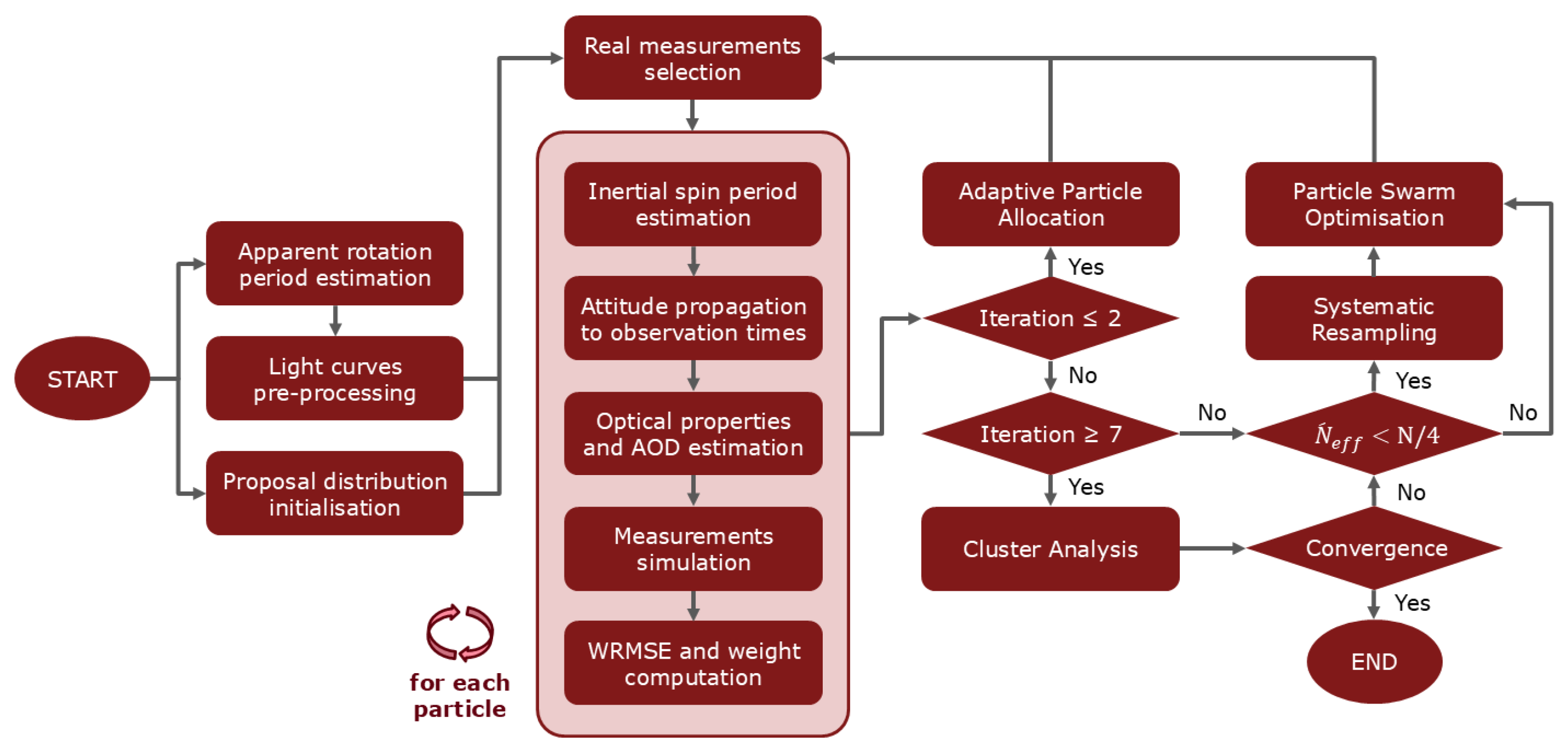
Figure 1. AISwarm-LS light curve inversion algorithm.
Aerospace 12 00942 g001
Figure 2. Light curve pre-processing to build the global bins of measurements.
Aerospace 12 00942 g002
Figure 3. Effect of the inertial spin period on the light curve.
Aerospace 12 00942 g003
Figure 4. Effect of the diffuse reflection coefficient and the AOD on the light curve.
Aerospace 12 00942 g004
Figure 5. Satellite model.
Aerospace 12 00942 g005
Figure 6. Reference light curve.
Aerospace 12 00942 g006
Figure 7. Particle distribution evolution during the AISwarm-LS execution.
Aerospace 12 00942 g007aAerospace 12 00942 g007b
Figure 8. Comparison of estimated and reference light curves.
Aerospace 12 00942 g008
Figure 9. Relative error between the estimated and reference light curves.
Aerospace 12 00942 g009
Table 1. Reference attitude, optical and atmospheric parameters.
Attitude parametersYaw [deg]34
Pitch [deg]63.5
Roll [deg]–28
Spin axis azimuth [deg]165
Spin axis elevation [deg]83.5
Spin period [s]60
Optical and
atmospheric
parameters
k d , ± X B [–]0.5
k d , ± Y B [–]0.15
k d , ± Z B [–]0.85
AOD [–]0.2
Table 2. Results of the light curve inversion method.
ReferenceWeighted Cluster
Estimate
Final Estimate
(LM + BOBYQA)
Attitude parametersYaw [deg]3432.906 ± 2.02632.406
Pitch [deg]63.562.670 ± 1.19662.919
Roll [deg]–28–26.393 ± 1.247–27.959
Azimuth [deg]165159.903 ± 2.869162.204
Elevation [deg]83.584.047 ± 0.45083.552
Spin period [s]6060.043 ± 0.03760.046
Optical and
atmospheric
parameters
k d , ± X B [–]0.50.455 ± 0.0190.481
k d , ± Y B [–]0.150.161 ± 0.0070.149
k d , ± Z B [–]0.850.819 ± 0.0450.829
AOD [–]0.20.178 ± 0.0230.186
WRMSE [–]1.1731.008
Table 3. Computational performance of the AISwarm-LS method.
Average Time
Light curve pre-processing1.16 s
Measurements simulation497.2 s
LSM for k d , Γ and AOD estimation0.55 s
Inertial spin period estimation0.41 s
WRMSE and weight computation1.53 s
Adaptive Particle Allocation47.3 s
Systematic Resampling0.052 s
Particle Swarm Optimisation0.58 s
Clustering245.3 s
Cluster refinement74.8 s
Total time85.3 min
Disclaimer/Publisher’s Note: The statements, opinions and data contained in all publications are solely those of the individual author(s) and contributor(s) and not of MDPI and/or the editor(s). MDPI and/or the editor(s) disclaim responsibility for any injury to people or property resulting from any ideas, methods, instructions or products referred to in the content.