Article

Aerodynamic Performance of a Natural Laminar Flow Swept-Back Wing for Low-Speed UAVs Under Take Off/Landing Flight Conditions and Atmospheric Turbulence

by
Nikolaos K. Lampropoulos
1,*,
Ioannis E. Sarris
2,
Spyridon Antoniou
3,
Odysseas Ziogas
3,
Pericles Panagiotou
3 and
Kyros Yakinthos
3
1
Hellenic Air Force Academy, Dekelia Air Base, Acharnes Attikis, 13671 Tatoi, Greece
2
Department of Mechanical Engineering, University of West Attica, 250 Thivon P. Ralli Str., 12241 Athens, Greece
3
Laboratory of Fluid Mechanics and Turbomachinery, Department of Mechanical Engineering, Aristotle University of Thessaloniki, 54124 Thessaloniki, Greece
*
Author to whom correspondence should be addressed.
Aerospace 2025, 12(10), 934; https://doi.org/10.3390/aerospace12100934 (registering DOI)
Submission received: 31 August 2025 / Revised: 8 October 2025 / Accepted: 14 October 2025 / Published: 16 October 2025
(This article belongs to the Section Aeronautics)

Abstract

The topic of the present study is the aerodynamic performance of a Natural Laminar Flow (NLF) wing for UAVs at low speed. The basis is a thoroughly tested NLF airfoil in the wind tunnel of NASA which is well-customized for light aircrafts. The aim of this work is the numerical verification that a typical wing design (tapered with moderate aspect ratio and wash-out), being constructed out of aerodynamically highly efficient NLF airfoils during cruise, can deliver high aerodynamic loading under minimal freestream turbulence as well as realistic atmospheric conditions of intermediate turbulence. Thus, high mission flexibility is achieved, e.g., short take off/landing capabilities on the deck of ship where moderate air turbulence is prevalent. Special attention is paid to the effect of the Wing Tip Vortex (WTV) under minimal inflow turbulence regimes. The flight conditions are take off or landing at moderate Reynolds number, i.e., one to two millions. The numerical simulation is based on an open source CFD code and parallel processing on a High Performance Computing (HPC) platform. The aim is the identification of both mean flow and turbulent structures around the wing and subsequently the formation of the wing tip vortex. Due to the purely three-dimensional character of the flow, the turbulence is resolved with advanced modeling, i.e., the Improved Delayed Detached Eddy Simulation (IDDES) which is well-customized to switch modes between Delayed Detached Eddy Simulation (DDES) and Wall-Modeled Large Eddy Simulation (WMLES), thus increasing the accuracy in the shear layer regions, the tip vortex and the wake, while at the same time keeping the computational cost at reasonable levels. IDDES also has the capability to resolve the transition of the boundary layer from laminar to turbulent, at least with engineering accuracy; thus, it serves as a high-fidelity turbulence model in this work. The study comprises an initial benchmarking of the code against wind tunnel measurements of the airfoil and verifies the adequacy of mesh density that is used for the simulation around the wing. Subsequently, the wing is positioned at near-stall conditions so that the aerodynamic loading, the kinematics of the flow and the turbulence regime in the wing vicinity, the wake and far downstream can be estimated. In terms of the kinematics of the WTV, a thorough examination is attempted which comprises its inception, i.e., the detachment of the boundary layer on the cut-off wing tip, the roll-up of the shear layer to form the wake and the motion of the wake downstream. Moreover, the effect of inflow turbulence of moderate intensity is investigated that verifies the bibliography with regard to the performance degradation of static airfoils in a turbulent atmospheric regime.

1. Introduction

The capability of the wing to keep the flow laminar over large part of its surface is key in enhancing its aerodynamic performance. For the category of light aircrafts at low speeds, Mach ≈ 0.1, NASA designed the the NLF(1)-0416 airfoil which keeps the flow over large parts of its surface laminar. The use of this airfoil for the design of typical wings for low-speed UAVs seems quite promising; nevertheless, the aerodynamic efficiency and safety of an industrially relevant wing must be verified numerically before testing. To this end, a CFD code that models or predicts the transition must be used in order to quantify the gain by keeping the flow laminar. Apart from performance, it must be verified that the typical wing design can either retain much of its lift capability at high AoA even if the laminar flow is not achieved, e.g., due to insect contamination, and the laminar separation bubble on the suction side of the wing finally is suppressed and the boundary layer becomes turbulent as it happens in the wind tunnel test. Otherwise, if the bubble continues growing without reattachment of the flow on the wing, an abrupt separation and stall may happen. With regard to transition modeling, an option is the incorporation of the e n method (see van Ingen [1]) in the code or the use of RANS models, such as the one proposed by Langtry and Menter [2], which are compatible with modern CFD codes running on massively parallel computers. These models have a degree of efficiency since a swept-back wing at high AoA produces a strong WTV which promotes spanwise flow, e.g., three-dimensional effects that have been shown to have an effect, and an increase in sweep angle leads to higher amplification rates and faster transition; see Fischer [3]. On the other hand, the selection of a Direct Navier–Stokes solver or Large Eddy Simulation (LES) model for the identification of the transition is not applicable at the range of a couple of million Reynolds number flow around a UAV wing. An interesting alternative, which is used in the current work, is the IDDES turbulence model [4] which has already been used successfully for boundary layer transition, at these Reynolds numbers, in the bibliography by Verhoefen [5].
Apart from its transition capability, IDDES has higher accuracy than RANS models to simulate the WTV inception and formation which is also within the scope of the current work. Its correct prediction concerns the aerodynamic efficiency of the wing itself, the stability of the aircraft if the WTV interacts with the empennage and stability issues to the following aircrafts. With swept-back wings, the effect of WTV is more pronounced on the following grounds: the aft movement of the aerodynamic center by wing aft sweep raises the lift force on the outer panel relative to the inner one according to Sadraey [6]. This results in the amplification of the WTV and subsequently of the spanwise flow, which, in turn, causes the thickening of the boundary layer in the wing tip region; hence, this area becomes more susceptible to stall. By increasing the AoA even further, the aerodynamically inactive, stalled region expands from tip to root (Soltani et al. [7]); thus, the center of pressure moves forward inducing the wing pitch-up tendency (Antoniou et al. [8]). It is worth mentioning that the WTV-induced spanwise flow from root to tip due to low pressure in the vortex region also results in lift reduction since the inclination of the freestream velocity vector reduces the component parallel to airfoil chord which is capable of producing lift. Moreover, any lateral motion contributes to additional skin friction drag and wasted kinetic energy. The negative effect of WTV can also be attributed to the reduction of α e f f in the vicinity of the leading edge which results not only in lower lift but also in the aft tilt of the lift vector, thus producing the so called induced drag. Therefore, the mitigation of the WTV is a major concern in the design phase of low-speed/swept-back and relatively short wings.
In terms of the computational methods that simulate the WTV, there is a series of approaches spanning from the least to very accurate but computationally intensive methods. The former is typically the unsteady Navier–Stokes equations with linear eddy viscosity turbulence models (URANS), and the latter are either the Large Eddy Simulation (LES) for academic or low Reynolds number flows, or the Detached Eddy Simulation (DES) for industrial applications. In this context, O’Regan et al. [9] investigated the near-field development of a WTV at two angles of attack (AoA) (five and ten degrees) for a square tip NACA0012 wing at chord Reynolds number R e c   =   3.25  ×  10 5 . It was proven that both models (URANS and LES) predicted the mean flow for A o A = 5 0 reasonably well, but URANS greatly underpredicted the mean flow for A o A = 10 0 , and the level of turbulence levels at all downstreams locations. On the contrary, the LES model could identify the jet-like axial velocity surplus in the wake and match the experimental value even at ten degrees. This is due to the limitations of the Boussinesq approximation as it is applied by the linear eddy viscosity models within the highly rotational and anisotropic WTV. The concentration of the whole turbulent content in the eddy viscosity results in an overprediction of this factor which in turns leads to unrealistic numerical diffusion and increased decay rate as stated by Feder et al. [10]. An alternative to computationally intensive LES model is DES which can switch to LES model in the wake and circumvent the aforementioned deficiencies. Liang et al. [11] intercompared DES and RANS-Spalart-Allmaras (RANS-SA) results with experiments finding the NACA0012 rectangular wing (Moderate Reynolds number and high AoA). They claimed that RANS-SA underestimated the highest value of axial vorticity in the WTV by 25–40%, whereas DES matched better with the experiment in terms of prediction of the streamwise vorticity. The underprediction of the WTV intensity is also verified by overprediction of minimum pressure in the WTV center. Li et al. [12] attempted an LES simulation for a NACA0012 airfoil wing with rounded wing tip at R e   =   4.6  ×  10 6 . They identified that the rotation of the WTV produces such low pressure in the core that can lead up to 2.0  ×  U axial surplus.
In terms of mesh requirement for implementation of the DES method around a wing within the range of one million Reynolds number, the bibliography provides the following information: Rogowski et al. [13] simulated the thick DU 91-W2-250 airfoil with a maximum thickness of 25 % for a big wind turbine using OpenFOAM® v2112 and the DES model with the transition SST turbulence model. The mesh size was Δ x + 900 , Δ y + 1 and Δ z + 800 . They managed to predict transition, but this can be attributed to the transitional RANS model which is incorporated in DES. Mitchel et al. [14] attempted a DES analysis of a delta wing aiming at the identification of vortical substructures in the shear layers that are formed near the apex of the wing. The flow conditions were high AoA at Reynolds numbers close to one million. They claimed that the DES model proposed by Spalart-Allmaras was implenented on meshes having a surface resolution 200 times larger than the wall normal direction.
Regarding the aerodynamic analysis of low-speed NLF wings with advanced turbulence modeling, the bibliography is very limited. Pereira et al. [15] investigated an unswept wing with the NLF(1)-1015 airfoil at low speed (Mach = 0.1–0.3). The CFD code was the Lattice Boltzmann software XFlow by Dassault Systèmes [16]. The turbulence model was the Wall-Adapting Local-Eddy-viscosity (WALE) which is a computationally more economical variant of LES. The NLF wing produced an increase in efficiency, in comparison to the NACA4615 wing, from roughly 5 % at Mach = 0.1 to over 15 % at Mach = 0.25.
In this context, the objective of the present computational study is complementary to the aforementioned bibliography since it attempts the identification of inception, evolution and decay of the WTV under low turbulence levels for a moderate aspect ratio swept-back wing at low speeds. The selected flight condition, as tabulated in Table 1, is the high AoA/take off or landing regime by which the WTV is expected to be more prominent. The Navier–Stokes equation solver uses turbulence modeling of both engineeering and high-level accuracy. Four different models are used herein which either model/resolve the transition of the flow from laminar to turbulent or consider the flow full turbulent. Regarding the methods that estimate the transition points on airfoils and activate the turbulent models, it is the temporarily steady two-dimensional RANS model of Langtry and Menter [2], named as kOmegaSSTLM. In terms of transient simulations, three models are used which are the following: the unsteady RANS model as initially proposed by Spalart and Allmaras [17] and the IDDES as as proposed by Shur at al. [18] which differs considerably in the treatment of turbulence. While the former estimates the Reynolds stresses through the Boussinesq approximation, namely by considering them as proportional to eddy viscosity and the mean strain rate, the latter switches modes between DDES in the inner region of the boundary layer, where a highly stretched mesh is used, and WMLES in the shear layer and wake region, where the use of uniform and very dense meshes is feasible. In this way, the regions where the wing tip vortex is generated and evolves are estimated by WMLES; namely the large eddies which carry most of the turbulent kinetic energy are resolved on the spatial and temporal scale of the flow, while the remaining regions are modeled through DDES. Finally, the dynamic k-equation LES model proposed by Kim and Menon [19] is used for high-level simulation of the flow around the natural laminar airfoil. This analysis is enhanced by introducing synthetic inflow turbulence as proposed by Poletto et al. [20] so that realistic atmospheric conditions, i.e., values of intermediate turbulence levels (≈2%), are considered. Such conditions can be reproduced numerically by imposing a synthetic velocity field at the inlet of the computational domain. The practical interest of this simulation is the investigation of wing performance under considerable turbulent weather as complementary to minimal inflow turbulence CFD simulations which are common practice for industrial applications. For example, the rotation speed V R , which is the speed at which the crew makes a control input with the intention of lifting the aircraft out of contact with the runway, must be well above the stall speed so that the aircraft can take off even at conditions of intermediate turbulence. Moreover, the propulsion system must be capable of producing enough thrust to counteract the high induced drag which is developed during take off at high AoA under turbulent weather. Vertical take off of a drone from the deck of a frigate is also of interest since the wings encounter a complex airflow being generated in the wake of the bluff body, such as the ship. The aforementioned applications are supported by the CFD code OpenFOAM® [21] which is exclusively used herein. The computational meshes were produced by a commercial mesh generation while the computations were executed on the HPC platform ARIS.
This paper has the following structure: it initially attempts benchmarking of the IDDES model with wind tunnel results of the airfoil. By making use of a highly dense mesh (used for LES simulation), as well as a coarser one with mesh density close to the 3D wing simulation, it is verified that the method produces aerodynamics metrics close to the experiment while the transition points are well-predicted. Results of additional models such as the LES and kOmegaSSTLM are presented to verify the CFD solver. Subsequently, a comprehensive study of the flow around the wing at minimal freestream turbulence is executed in order to prove grid sensitivity of the code with different type of meshes. The prediction of the transition line on both sides of the wing is also illustrated and explained. The kinematics of the flow in the near wing is identified in order to verify that the wing adheres to the standards of the wing design bibliography. The inception, formation and evolution of the wing is examined in detail in order to estimate the WTV’s strength and coherence in the near- and far-field downstream. Finally, the wing is investigated under an intermediate freestream turbulence regime which is constructed with a synthetic turbulence model generator. The aim is the verification of performance and safety (avoidance of high lift mitigation or abrupt stall) with a more realistic unsteady CFD solver. Intercomparison with conventional RANS models is also executed.

2. Material and Methods

2.1. Geometry of the Wing and Airfoil Selection: Benchmarking of the CFD Code

The airfoil used for the wing development is the NLF(1)-0416 Natural Laminar Flow (NLF) which is developed by NASA and being extensively tested in the Langley Low-Turbulence Pressure Tunnel [22]. The airfoil which targets low-speed, light, single-engine aircrafts aims to keep the flow laminar through an extensive part of both pressure and suction side while it exhibits a high C l , m a x and profile drag at cruise lift coefficient of 0.4 comparable to NACA 6-series airfoils. The airfoil was investigated numerically with the current code in order to validate the method against the experimental results. The flow conditions and simulation details are tabulated in Table 2, respectively. The 2D mesh is a typical O-type with about 160 points on each side of the airfoil while high aspect ratio cells are used near the wall so that the condition y + < 1 is observed. The 3D mesh is a very dense LES-type mesh which is an O-type around the airfoil with 60 inflation layers being subsequently extruded in 70 layers spanwise. The span is 0.1 × chord wide so that the boundary layer is fully developed near the trailing edge. This enables the proper application of periodic boundary conditions spanwise. A total of 800 points are put on each side of the airfoil while 40 points are put lower on the blunt trailing edge; see Figure 1. According to the flat plate theory, the expected y + = 1 corresponds to a cell size on the wall equal to d s = 2.3 × 10 5 m. Under this assumption, the 3D mesh sizing reads as follows: Δ x + 50 , Δ y + < 1 and Δ z + 60 are close to the limits proposed by Piomelli U. and J.R. Chasnov J.R. [23] so that the coherent turbulent structures can be captured in a wall-resolved LES. In terms of discretization of the convective term, a second-order bounded Total Variation Diminishing (TVD) scheme is used for high accuracy IDDES (NLF3) and LES (NLF4) simulations, whereas a second-order upwind scheme is preferred for RANS simulations (NLF1 and NLF2). The time step is d t = 1 × 10 3 s for NLF2, d t = 5 × 10 5 s for NLF3 and d t = 3 × 10 6 s for NLF4.
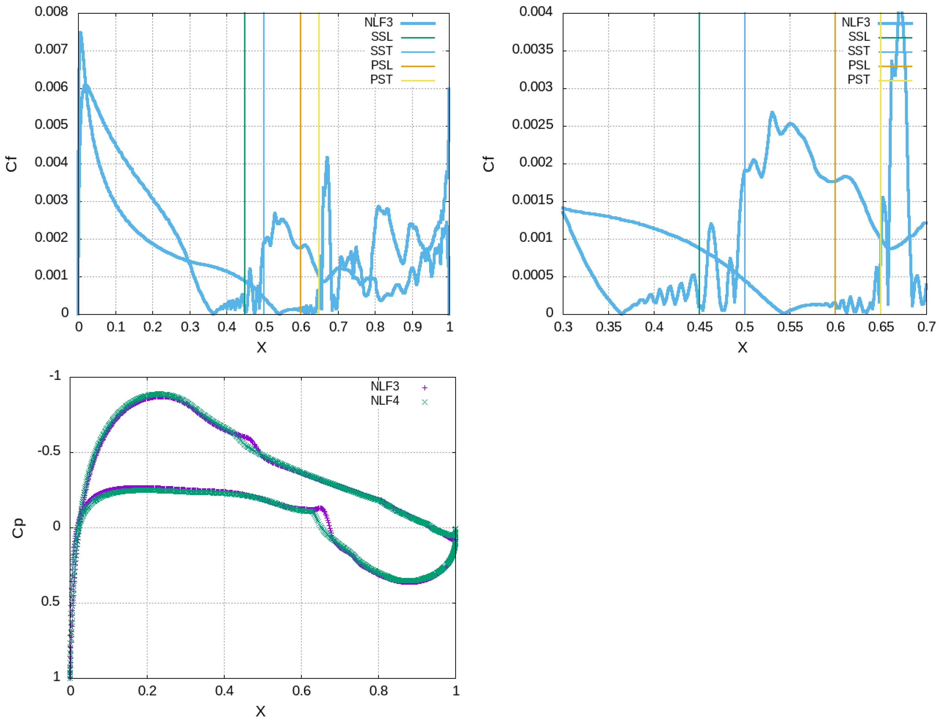
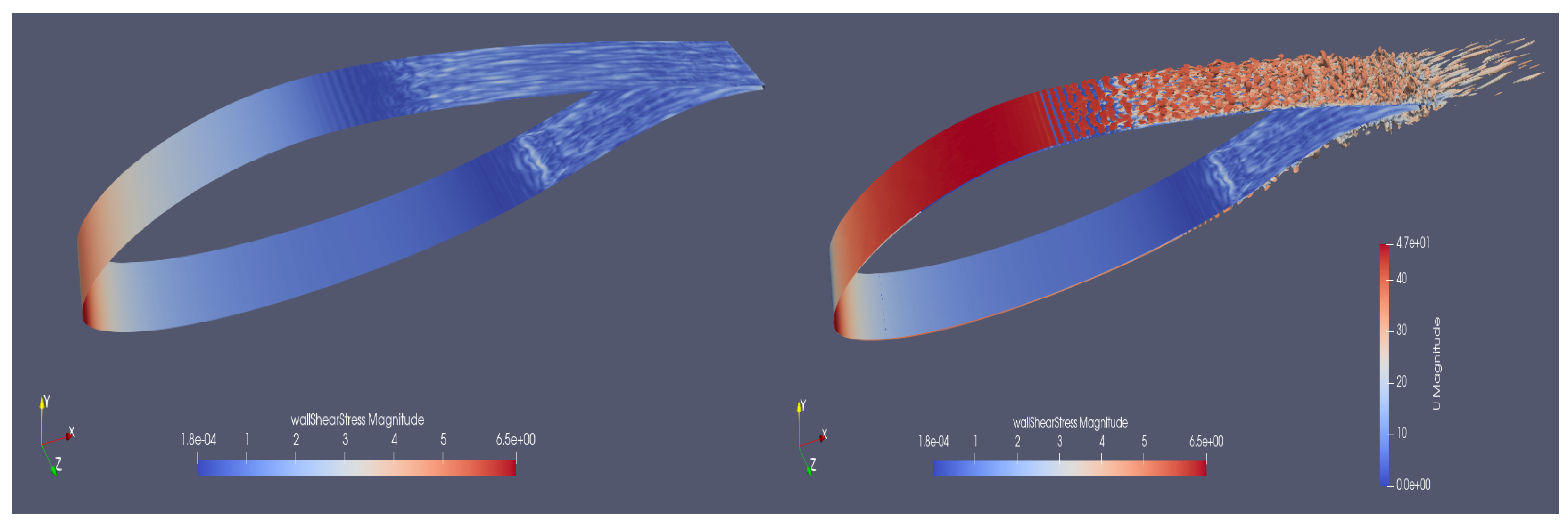
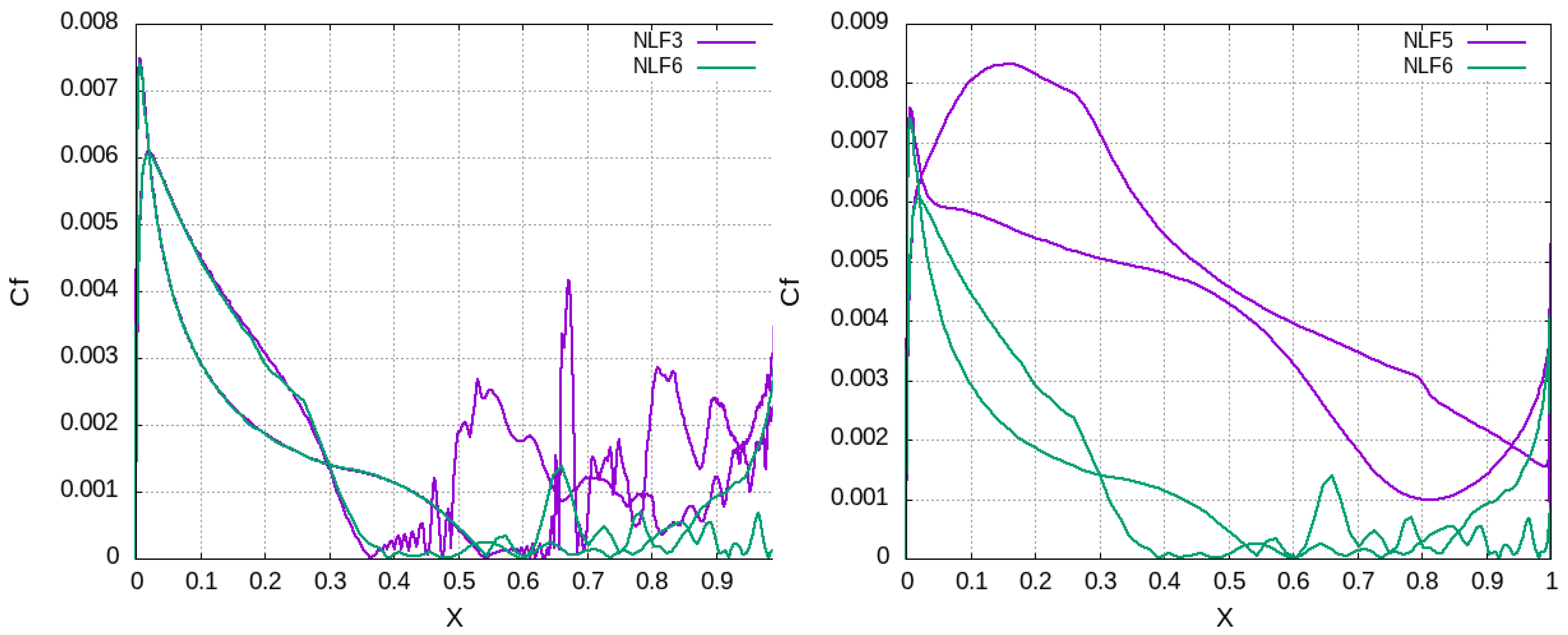
The numerical results are benchmarked against the findings of the wind tunnel experiment [22]; see Table 3. On the experimental results, low-speed wind tunnel boundary corrections have been applied so that a direct comparison with isolated airfoil CFD simulation is enabled. The experimental data comprise C l and C d coefficient results as well as the positioning of transition to turbulence (as percentage of chord) by use of microphone measurements. In the three-letter terminology, PS stands for Pressure Side, SS for the Suction Side, L for Laminar and T for Turbulent. With regard to the NLF1 simulation (see Table 3, Figure 1, a good match with the experiment in terms of both force coefficient and transition prediction, see spikes in C f distribution. On the contrary, the NLF2 method underpredicts the lift and overpredicts the drag since no transition model is used; thus, errors are introduced through the activation of the turbulence model from the leading edge of the airfoil. More accurate results are produced by NLF3 which resolves the turbulence and the mechanisms of transition as being verified by the C f distribution (see Figure 2), where a smooth distribution (Laminar region) is followed by a resonant one (instabilities) and finally an oscillatory one (turbulent). It is worth mentioning that the IDDES method (NLF3) which is used in the subsequent 3D simulation around the wing is capable of resolving the transition, as also identified by the kinks in Cp distribution (see Figure 2), while it is numerically stable with large time steps, i.e., d t = 5 × 10 5 , which are realistic for industrial applications. The difference between resolution of transition (NLF3) and prediction (NLF1) is depicted in Figure 3 where NLF3 produces realistic wall shear stress distributions whereas NLF1 activates the turbulence model downstream of the predicted transition point. The most advanced method used herein is NLF4 (wall resolved LES) which produces instabilities that are evident in Figure 4 where the Q-criterion isosurface for vortex visulization is depicted. The capabilities of the code on coarse meshes to be used around the wing are tested in cases NLF5 and NLF6. As depicted in Figure 5 and Figure 6, NLF6 (IDDES, coarse) can predict the transition close to the points identified by NLF3 (IDDES, dense), although it underestimates the wall shear stress in the turbulent region. Nevertheless, the laminar parts also have identical stress which is much smaller than the one predicted by NLF5 (URANS-SA, coarse). The aerodynamic metrics in Table 3 verify that NLF6 produces results close to experimental data, whereas the RANS-SA simulations underestimate lift and considerably overestimate drag since they do not predict the laminar part of the flow.
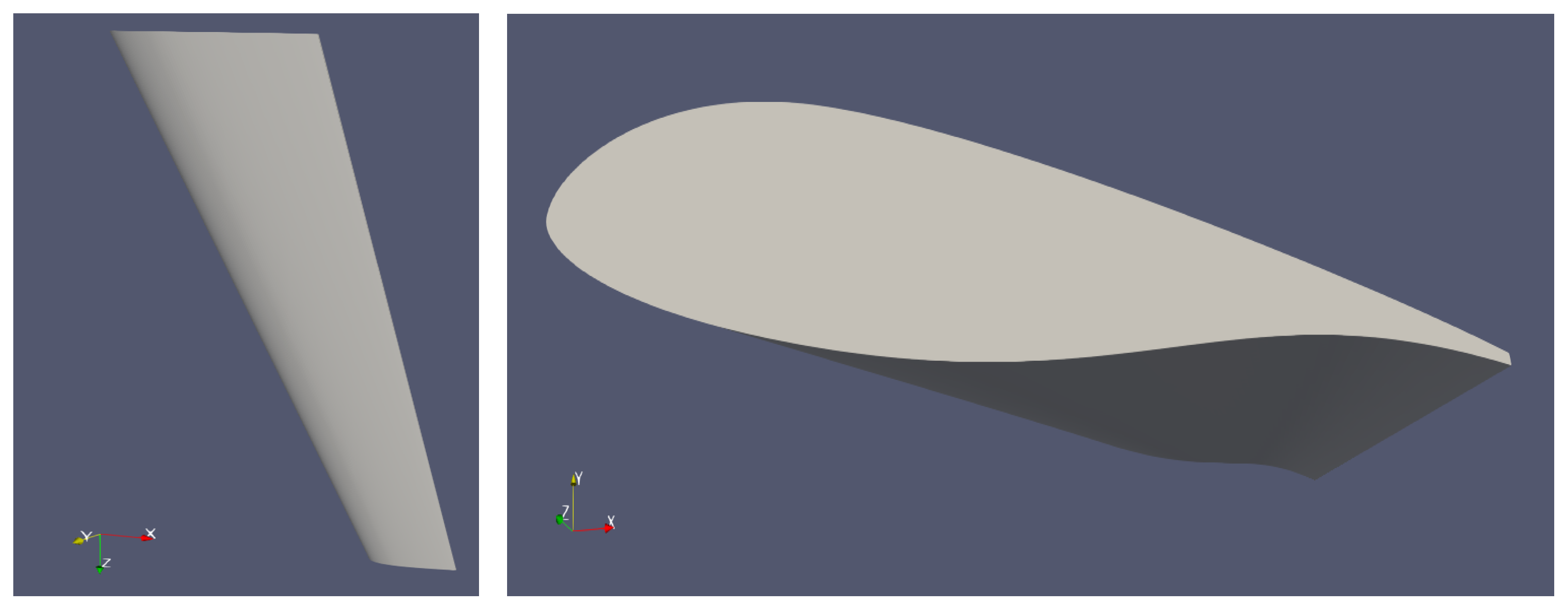
On the basis of the preceding analysis and the guidelines for wing design provided by Raymer [24], a wing for a low-speed light aircraft is designed (see Figure 7), whose geometrical details are tabulated in Table 4. In a nutshell, it is a moderate aspect ratio swept-back wing for blended wing body aircrafts with zero incidence angle at the root and four degrees twist. This value is selected for safety reasons (the outboard section of the wing remains aerodynamically active even if the inboard sections is stalled). Moreover, with twisting of the wing, the ideal spanwise elliptical lift distribution is pursued, aiming at the mitigation of the wing tip vortex. To this end, this twist angle is also chosen since the zero lift AoA of the airfoil is A o A = 4 0 ; therefore, the wing tip is expected to be minimally loaded during cruise flight ( A o A = 0 0 ) which results in a weak WTV. The three degrees anhedral conduces to the reduction in swept-back wing lateral stability, which, when being excessive, may lead to dutch roll-type dynamic instabilities.

2.2. CFD Simulation and Turbulence Modeling

The turbulent flow is simulated herein through a transient in-time simulation by making use of the Improved Delayed Deatched Eddy Simluation (IDDES). This is based on the baseline RANS-Spalart-Allmaras one-equation turbulence model which solves a transport equation for the viscosity like variable ν ˜ . This model switched modes between DDES (inner boudary layer region) and WMLES (outer boundary layer and beyond). Thus, the flow in the inner region of the boundary layer is better resolved than RANS models, and instabilities that result in transition of the boundary layer can be identified. Moreover, WMLES resolves the large vortical structures in the boundary layer and beyond where the near-cubic-sized hexahedra have comparable size with the large eddies which carry about 70 to 80% of turbulence. The size of these eddies is the integral length scale which has the magnitude of some hundredths of the characteristic length of the flow, e.g., the airfoil chord. Since the eddy is a spiral motion which can be identified adequately with four cells in two and eight cells in three dimension, it is readily deduced that an LES-type mesh in the near-wake and beyond is feasible even for industrial wall-bounded flows of Reynolds number in the order of several millions, as it is the present case.
A further extension of this method is attempted herein by introducing synthetic inflow turbulence as proposed by Poletto et al. [20], aimimg at resembling the atmospheric turbulence. The inlet conditions are a divergence-free turbulence field that can reproduce almost all possible states of Reynolds stress anisotropy. The simulation consists of two distinct phases. Initially, synthetic turbulence is generated on a virtual rectangular structured-mesh plane by solving steady state RANS. Thus, the Reynolds stress tensor, the velocity field and the integral length scale, e.g., the average size of the largest, energy-containing eddies, are estimated for the devoloped flow in a rectangular duct, being of the size of the aerodynamic wing tunnel. Subsequently, these quantities are mapped on the inlet plane of the computational domain that contains the wing, and velocity fluctuations are reproduced by means of these quantities and appropriate shape functions. Finally, these fluctuations are superimposed to the baseline velocity which is already estimated through the precursor RANS simulation. In this way, fictitious eddies entering the domain can produce a divergent free-flow field, e.g., constant mass flow rate, at inlet that guarantees that the incompressible solver does not produce unrealistic pressure fluctuations on the aerodynamic body during the unsteady simulation. The latter unfavorable solution is reached in case that a white noise, that is, chaotic signal of velocity, is imposed at the inlet of the aerodynamic wind tunnel since this boundary condition is inappropriate for incompressible CFD solvers that have constant pressure boundary condition at the exit. This synthetic eddies generation is computationally inexpensive since the precursor mesh is very small and the simulation runs once. Moreover, the method is user-friendly since the flow speed and the turbulence level of the constructed flow field can be set by imposing the appropriate boundary conditions for velocity, k (turbulent kinetic energy), and ϵ (dissipation of k).
In terms of computational meshes, three grids are used herein (see Figure 8), whose characteristics are tabulated in Table 5. The grid is a wind tunnel type design where the semi-span of the wing is simulated. About 200 points are placed in each side of the airfoils and 350 points are used spanwise. A total of 30 points are used in the blunt/cut-off trailing edge in order to develop 60 high orthogonality inflation layers with hyperbolic extrusion. Two meshes of different mesh density in the vicinity of the wall are constructed for the simulations S1 and S2 so that the grid independence of results is examined. The regions of the mesh where the wake and the WTV are expected to emerge are also densely populated. The size of the cells is selected through a prior estimation of the dimension of the turbulence length scale by executing a R A N S ( k ϵ ) model simulation and subsequently using Equation (1). This results in a diameter L T = 0.02 m which is the size of large eddies carrying most of energy contents, which are meant to be resolved by an adequately dense isotropic mesh. The cell size in highly turbulent regions is selected to be about 5 mm and the time step d t = 5 × 10 5 s, which is expected to be small enough for the accuratate temporal resolution of vortices (LES regions) while it ensures the numerical stability of the DDES mode in the highly stretched mesh region near the wall boundary. Special attention is given in the wing tip and near wake region, up to one tip chord downstream, where nearly cubic cells are achieved. Thus, the switch of the turbulence model to LES mode is enabled in order to capture the phenomenon of wake formation and the downwash.
Regarding the S3 case, a different meshing strategy is selected. This comprises the structured mesh with the inflation layers around the wing and a series of cartesian-type isotropic structured meshes of decreasing density in the direction away from the wing, which are interconnected with layers of pyramids. This so-called Voxel-type meshing strategy enables the transportation of synthetically constructed eddies at the inlet throughout the domain, thus retaining a large portion of the inflow turbulence. The time step for the S3 case is selected to be d t = 1 × 10 3 s since a large physical time span must be simulated.
ϵ = C m 3 4 k 3 2 L T
In terms of the CFD solver it uses a second-order implicit backward temporal discretization scheme which implements the time marching by using the current and the two previous updated values of variables in the calculation of the temporal derivative. The convective terms are discretized by a second-order scheme which is a mix of linear and upwind methods, thus being a good compromise between accuracy (linear) and numerical stability (upwinding). The temporarily unsteady equations are solved by the PIMPLE algorithm which is a combination of PISO (Pressure Implicit with Splitting of Operator) and SIMPLE. This algorithm retains the numerical stability of the code, even at Courant numbers higher than one; thus, it is well-formulated for IDDES simulations on meshes with dozens of millions of computational cells which can be hardly handled even by HPC platforms. The method aims at the increase in the time step up to a value which enables the adequate temporal discretization of the vortical structures in the shear layer, the tip vortex and the wake where the WMLES mode is activated. At the same, time this time step must be small enough to enable WMLES to resolve the large vortical structures of the outer boundary layer and DDES for the instabilities in the buffer zone and the logarithmic part of the boundary layer. This model uses empirical blending function to switch between DDES and WMLES depending on the flow conditions and the grid resolution. It turns to WMLES when there is sufficient grid resolution and automatically switches to DDES when these requirements are not met [25]. Thus, it can capture the instabilities that trigger the transition of the boundary layer from laminar to turbulent. This was already reported in the master thesis of Verhoeven [5], who identified transition on the surface of a NACA0012 airfoil at zero angle of attack and Reynolds number of one million with the IDDES model of OpenFOAM®. The mesh resolution was 240 points on the suction side, 130 points on the pressure side and 34 cells in the spanwise direction, where the mesh thickness was equal to one tenth of the chord. It is worth mentioning that on some parts of the wing of the current study, the Reynolds number is even below one million since the effective velocity is reduced due to the sweep angle.

3. Results and Discussion

The numerical results are depicted in the form of Pressure Coefficient C p and Friction Coefficient C f distributions at several spanwise locations of the wing as well as the produced total lift and drag. The flow is illustrated by field distributions on cross-flow planes at axial positions in the wake and the WTV depiction along with the streamlines. The wake formation and stength is also estimated through flow field distributions in directions crossing the wake at several axial positions. The effective angle of attack as well as the downwash angle are estimated spanwise. For the minimal inflow conditions, the mean fields are obtained by averaging over a period of 1 s which corresponds to around 20 non-dimensional time units (one time unit is the time it takes for the flow to run 1 mean chord of the wing). This time window is estimated as adequate for obtaining statistically stationary results since the main aerodynamic performance metrics (lift and drag) are stabilized. On the contrary, the cases with inflow turbulence are extended to 7 s since the large time step affords such extended physical time simulations.

3.1. Take Off/Landing Flight Conditions Under Minimal Inflow Turbulence (Simulations S1 and S2) A o A = 12 0 , V = 20 m / s , ν = 1.5 × 10 5 m 2 / s

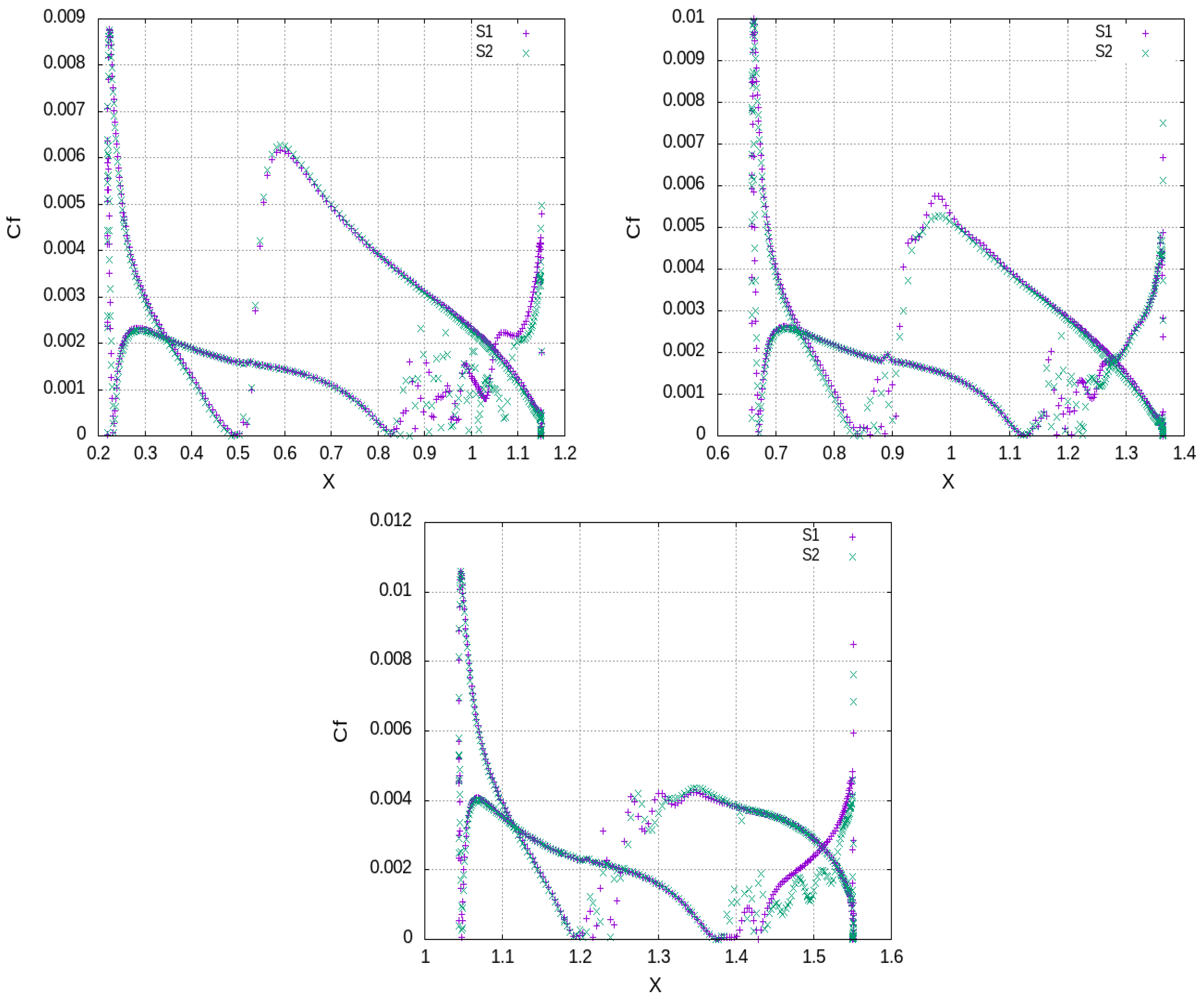
The analysis of the flow under low-speed take off/landing conditions is attempted through a detailed examination of the flow in the near-wing and in the wake for minimal inflow turbulence. The estimated performance of the wing for simulations S1 and S2 are depicted in Table 6. The grid independence of the results is identified through intercomparison of C p distributions (see Figure 9) and the wing aerodynamic metrics (Lift, Drag). The slight higher loading for S2 case is due to the higher spike in pressure at the leading edge which can be attributed to lower mesh density near the wall. The kinks in pressure distribution are accompanied by wall friction kinks, as depicted in C f distributions (see Figure 10), which are evidence of transition from laminar to turbulent flow. In terms of C f values on the suction side, the immediate drop after the peak on the leading edge hints at laminar flow which persists with a continuous drop up to the transition point where a spike is identified. Subsequently, the boundary layer becomes turbulent and the flow decelerates; thus, C f follows a continuous drop. On the pressure side, the laminar flow is more extended while an increase is observed in the cusp region. The differences in the predicted wall shear stress by the RANS and IDDES models is also depicted in Figure 11. By S0, the boundary layer is fully turbulent throughout the chord; thus, high skin friction is predicted. The results of S0 and S5 converge after the transition points. In terms of the pressure recovery in both sides of the airfoil, this is successful since the pressure distribution on both sides converges close to datum atmospheric pressure (zero value) at the trailing edge, thus inhibiting separation. The concave aft part of the airfoil in the pressure side leads also to deceleration of the flow/increase in pressure which enhances the produced lift.
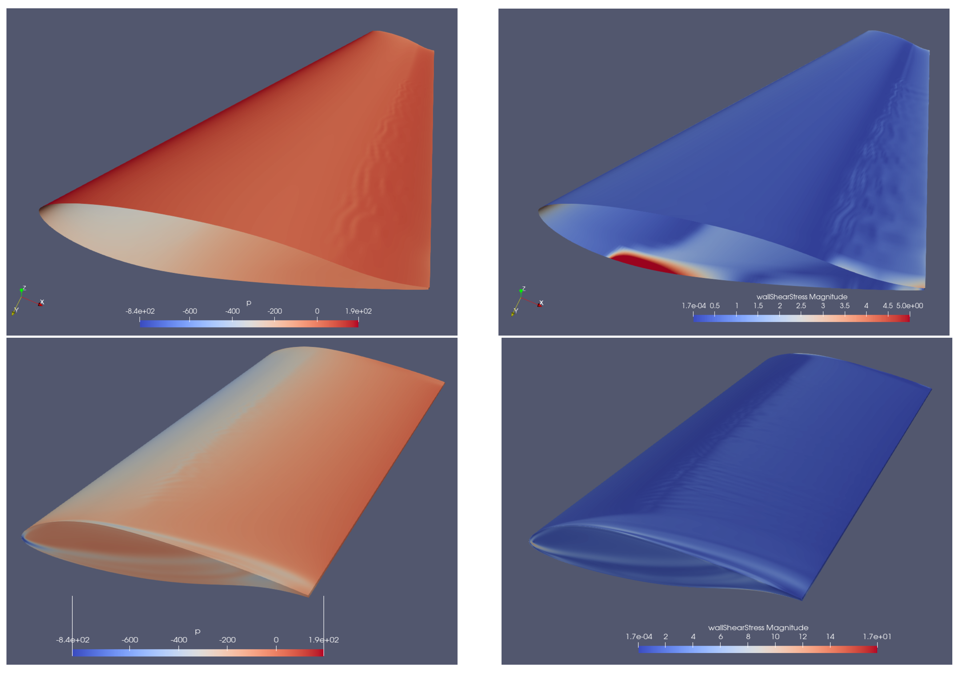
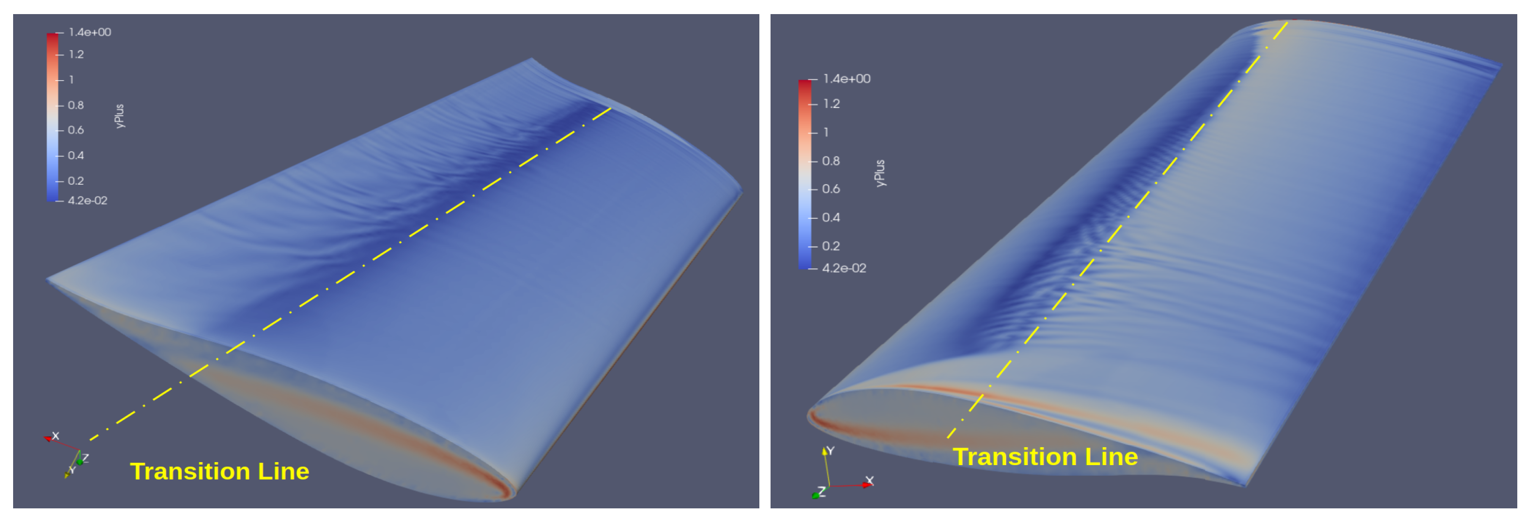
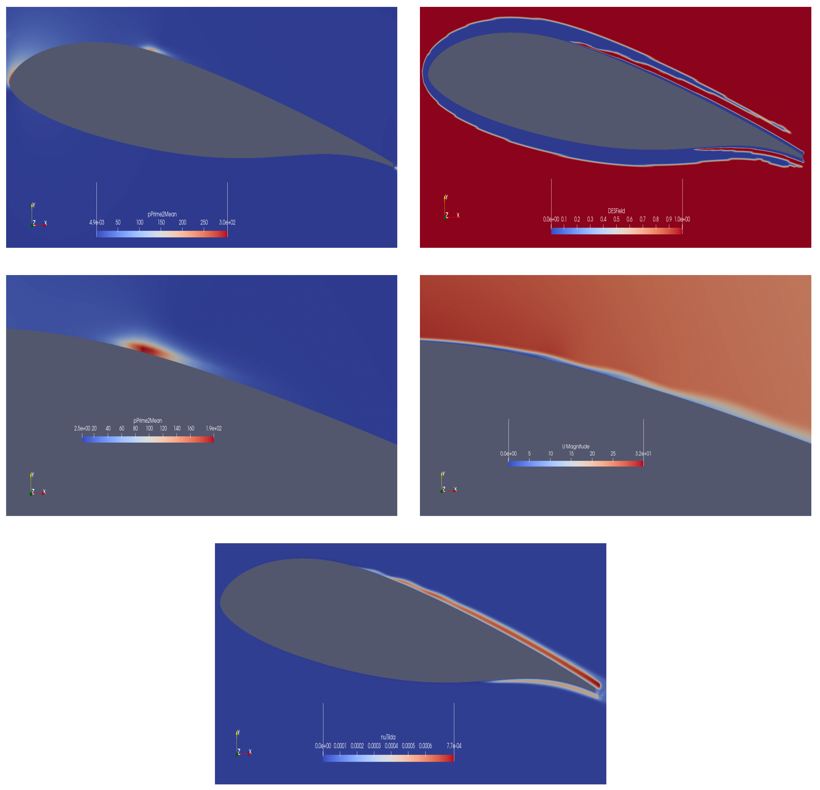
The ability of the method to predict transition is also verified by pressure and wall shear isosurfaces (see Figure 12) where faint instabilities are recognized. The transitional line is more pronounced in Figure 13 where a spike in y + distribution hints at an increase in wall shear stress. The mechanism of transition is depicted in more detail in Figure 14. A laminar separation bubble is formed on the suction side which is identified by the activity in pressure fluctuations. Subsequently, this bubble is suppressed and the boundary layer becomes fully turbulent as verified by its thickening. The distribution of the DESField metrics depicts how transition is identified by IDDES. In the near-wall region of the mesh, IDDES works on DDES mode. This is a dual RANS mode (very close to the wall, where turbulence is limited) and LES (in the remaining inner region of the boundary layer). As long as no flow disturbances are recognized, since the flow is laminar, the DDES mode persists. Once the disturbances emerge, IDDES switches to WMLES which is a purely LES variant (red color) that can resolve large vortical instabilities within the boundary layer and beyond. This results in the activation of the turbulence model in order to resolve the turbulent boundary layer (increase of ν ˜ ). In the near-wall, the mode remains DDES since WMLES cannot resolve the inner region due to low mesh density and the high aspect ratio of cells (persistence of blue color all over the near-wall region).

3.1.1. Analysis of the near-Wing Flow Under Minimal Inflow Turbulence (Case S2)

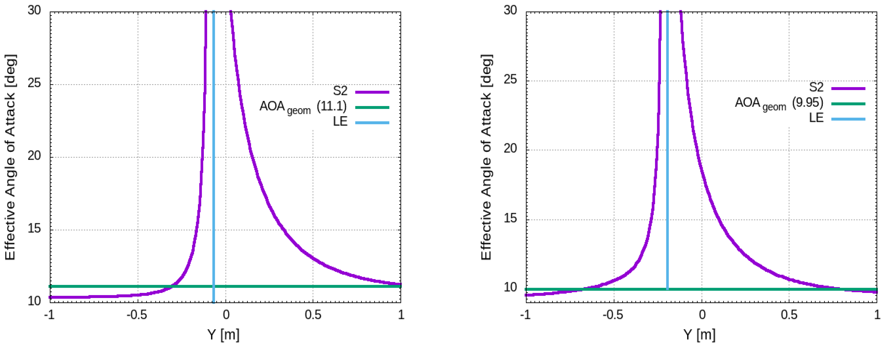
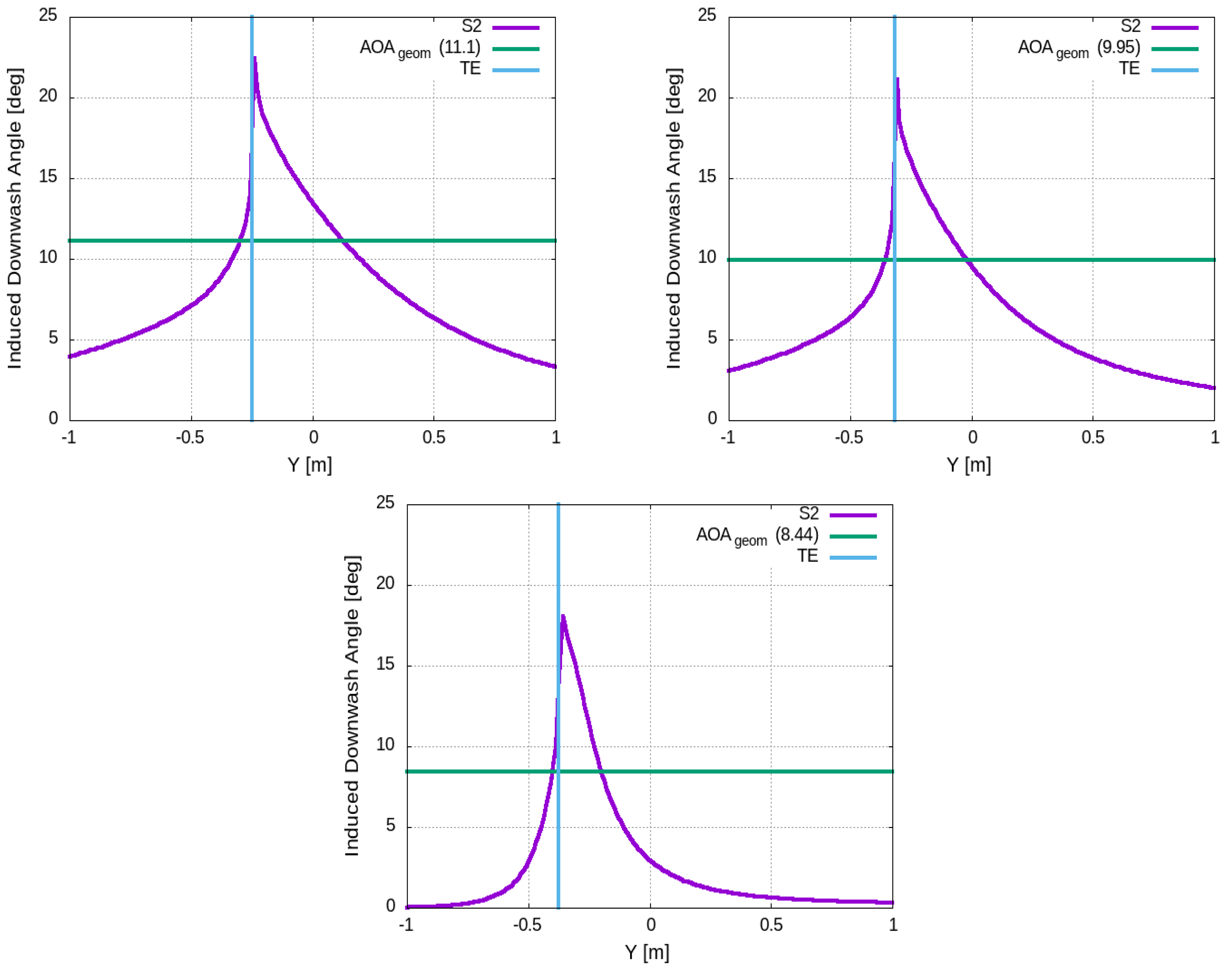
The pressure difference between the pressure and suction side of the wing give rise to a coherent WTV (see Figure 15). This is expected to be intense due to flow conditions (high AoA and low speed) as well as the significant spanwise flow, due to sweep angle, which conduces to vortex formation. This vortex induces in turn a spanwise diversion of the flow outboard on the pressure side and an inverse inboard diversion on the suction side (see Figure 15) (upper, left), which results in lower loading of the wing since the spanwise flow cannot produce lift, as well as in lost kinetic energy. Moreover, the WTV induces a downward diversion of the flow which reduces the AoA to α e f f (see Figure 16). This results not only in the reduction in lift but also in the inclination of the lift force, which is always perpendicular to local relative wing, to the rear; thus, the lift force vector conduces to drag, producing the so-called induced drag. This kinematics of the flow near the wing is depicted in Figure 17 where the angle α e f f is plotted along the dashed black line passing by the leading edge (see Figure 16) left at several spanwise positions. The geometric AoA, which reduces spanwise due to twist, is also depicted in the figure. The effect of the WTV on the incoming flow is identified by the reduction of α e f f at the position Y = 1 m, at both spanwise positions, below the geometric angle of attack of the airfoil. This is reasonably attributed to the WTV effect, e.g., the induced downwash to the freestream which reduces α e f f . In terms of the flow pattern after passing through the wing, we investigate it through the downwash angle ϵ (see Figure 16, right and Figure 18). The downwash angle is a function of the wing AoA ( α w ) and is determined in Sadraey [6] by Equation (2):
ϵ = ϵ 0 + ϵ α α w
In Equation (2), ϵ 0 stands for the downwash angle at zero AoA and ϵ α for the downwash slop with typical values of 1 degree and 0.3 degree/degree, respectively. In the current work, where A o A = 12 0 , a value of 5 degrees downwash is expected according to the prior analysis, while this value is expected to vary across the span and approach zero near the wing tip where the aerodynamic loading minimizes, as demonstrated by Raymer [24]. The results in Figure 18, across the dashed black line passing by the trailing edge (see Figure 16, right), are in conformity with the bibliography, since at the position Y = 1 m, the downwash angle is slightly below 5 degrees at 20 % of the semi-span, showing a tendency to reduce in the outboard direction up to zero value close to the wing tip. The downwash angle ϵ can also be estimated by Equation (3), and the induced angle of attack ( α i ) by Equation (4) (see Figure 16), as stated by Gudmundsson [26]. By substitution of C L = 1.147 into the last two equations, they yield ϵ = 5 . 13 0 and α i = 2 . 56 0 .
ϵ s i n ϵ = w V = 2 C L π A R
α i t a n α i = 1 2 w V = C L π A R
From the correlation A O A g e o m = A O A = α e f f + α i , and Figure 17, we can readily estimate α i at the position Y = 1 m, i.e., at about one mean chord from the leading edge at spanwise positions 20 % and 60 % which are tabulated in Table 7. Both estimations of α i are close to the theoritical value α i = 2 . 56 0 .

3.1.2. Analysis of the near-Wake Flow Under Minimal Inflow Turbulence (Case S2): Comparison of Near- and Far-Wake with RANS Predictions

The process of vortex formation is identified by examining flow quantities at several cross planes (see Table 8). The inception of the vortex starts as the emergence of two shear layers at the tip corners (see Figure 19), which circumvent the tip and merge. The high-level turbulence regions (shear layers) are wrapped, then they are mixed and gradually form a coherent vortex which is recognized downstream of the plane XC4. The process of shear layers wrapping is also depicted in Figure 20 where the minimum static pressure value defines the vortex center. Downstream of trailing edge, plane XC2, the minimum pressure increases and maximum cross-flow velocity decreases, hinting that the formed vortex loses quickly in strength. This is verified by the axial velocity contours (see Figure 21), where two chords downstream (plane XC6) the velocity range is between 18 m/s and 21 m/s, i.e., the freestream velocity is almost recovered. The maximuum axial velocity in the core at XC4 is equal to 31 m/s which represents a significant 1.5 × U i n f velocity surplus. The accelaration of the flow in the core gives rise to the wrapping of the shear layer and the suction of the air in the core which leads to a coherent vortex formation. Finally, the four-leaf clove pattern of the Reynolds shear stress v w ¯ is observed in Figure 22 where the Reynolds stress are shifted 45 deg from the corresponding mean strain rate. This phenomenon, which is also verified experimentally by Chow et al. [27] and numerically in a Large Eddy Simulation conducted by Jiang et al. [12], hints that the Boussinesq eddy viscosity assumption, which is the basis of isotropic linear eddy viscosity model, does not hold in the high anisotropic field of the WTV.
In terms of the vortex trajectory and strength, several quantities such as the pressure, axial velocity and normalized axial vorticity are plotted along a line being parallel to the y-axis passing through the core center at several cross-flow planes (see Figure 23). It is readily deduced that the vortex weakens quickly downstream since all quantities are reduced while the trajectory is not meandering, but points steadily towards the lift direction (increasing y-axis) and inboard (decreasing z-axis), as also depicted in Table 9. The WTV decay rate in terms of axial velocity surplus/deficit and turbulence intensity level is also examined through intercomparison of S0, S1 and S2 results which are tabulated in Table 6, where DR (Decay Ratio) stands for the ratio of axial to freestream velocity, hinting at either surplus (>1) or deficit (<1). The sampling is in the vortex center (as being identified by the minimum pressure at each cross plane) at several downstream positions, e.g., 0.5 m, 1.25 m and 3.25 m from the trailing edge of the tip airfoil. Both S1 and S2 predict an initial surplus which turns to a considerable deficit through a continuous deceleration in the WTV core. The mixing results in an increase in the turbulent content which amounts to T u 20 % at XC6, which is retained up to XC7. On the contrary, S0 identifies a continuous axial velocity deficit downstream (lower than S1, S2) and considerably lower turbulence levels. The considerable difference in RANS vs. IDDES models is readily attributed to the limitations of the Boussinesq assumption which estimates the Reynolds stresses through the mean strain tensor, which fails in the highly turbulent WTV. On the contrary, IDDES switches to LES in the wake, and thus, the turbulent flow is resolved in a purely unsteady manner where only the small eddies contribution is modeled through the subgrid scale viscosity. In this way, a small amount of artificial dissipation is introduced in the momentum equations which results in more realistic results. The practical implication of RANS modeling deficiencies for engineers is that the model underpredicts the authority loss of the empennage in pitching up the aircraft. As depicted in Figure 15, the WTV is coherent and widens downstream, while its trajector points inboard (see Table 9). IDDES predicts a velocity deficit of about 55 % and over 80 % for RANS at about 3 m downstream of the wing tip where the empennage may be mounted. Therefore, any part of the horizontal stabilizer and the elevator which are shadowed by the WTV will experience a considerable lift reduction, which is underestimated by the RANS simulation.

3.1.3. Aerodynamic Loading of the Wing by Intermediate Inflow Turbulence Levels

Following the preceding analysis, the aerodynamic performance of the wing is also investigated under take off/landing conditions under atmospheric turbulence conditions. To this end, the turbulent inflow is numerically reproduced by making use of the methodology proposed by Poletto et al. [20], i.e., by imposition of velocity fluctuations at the inlet of the computational domain so that a divergent free flow field is constructed. The baseline velocity and turbulence, being lumped in the form of turbulent kinetic energy, is calculated in prior through a RANS simulaton in a rectangular empty wing tunnel through recycling the exit flow to the inlet. Subsequently, the fluctuations being calculated on the basis of the integral length scale and the Reynolds stress tensor are superimposed to the RANS flow field to produce a a velocity front that travels through the computational domain. The time step is set at d t = 0.001 s so that a considerable physical time (7 s) simulation is feasible with the existing HPC resources. It is worth mentioning that the computational load with the synthetically produced inflow turbulence is about 20 times higher than the simulation with the constant velocity at inlet. This is due to the continuously changing velocity field which requires, within each time step, additional iterations so that the discretized mass and momentum equations can converge and stability of the algorithm is achieved. In this way, the transition phenomena on the wing cannot be identified; therefore, the boundary layer is assumed turbulent throughout the wing skin. Nevertheless, the imposition of the synthetically reproduced free stream is expected to reproduce more realistically the aerodynamically loading of the wing than the standar RANS models. The use of IDDES instead of RANS is also convenient in the sense that it enables the eddies to retain much of their turbulent content as they travel through the domain, whereas RANS would dissipate them due to the numerical dissipation of eddy viscosity.
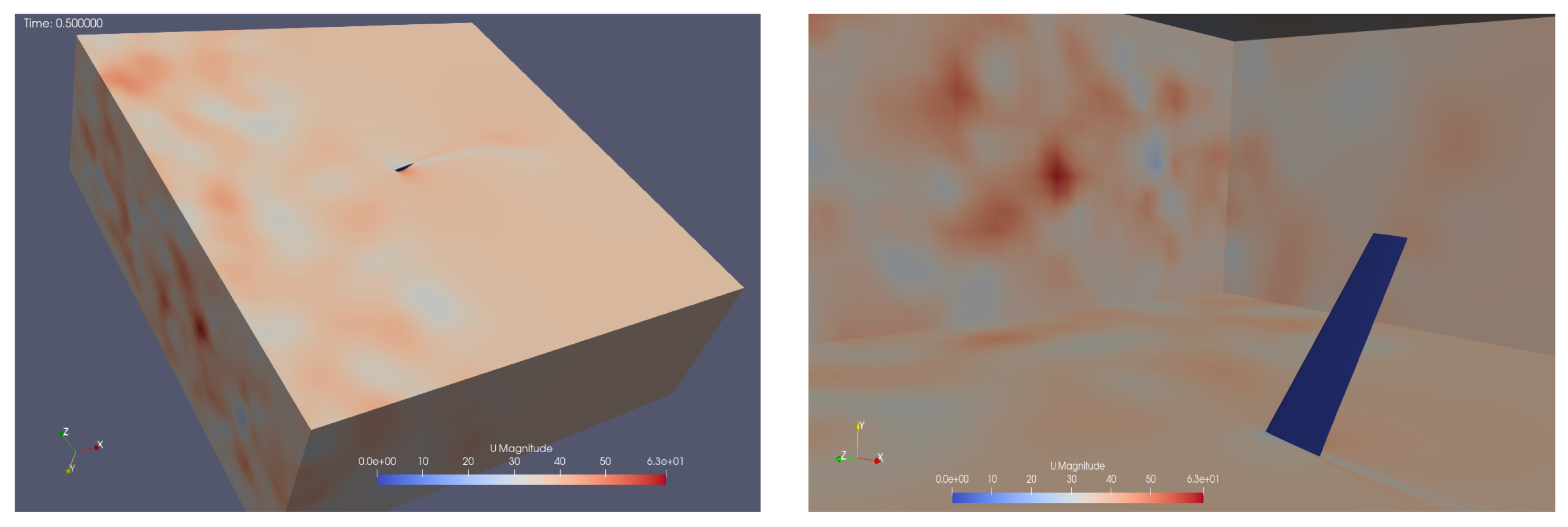
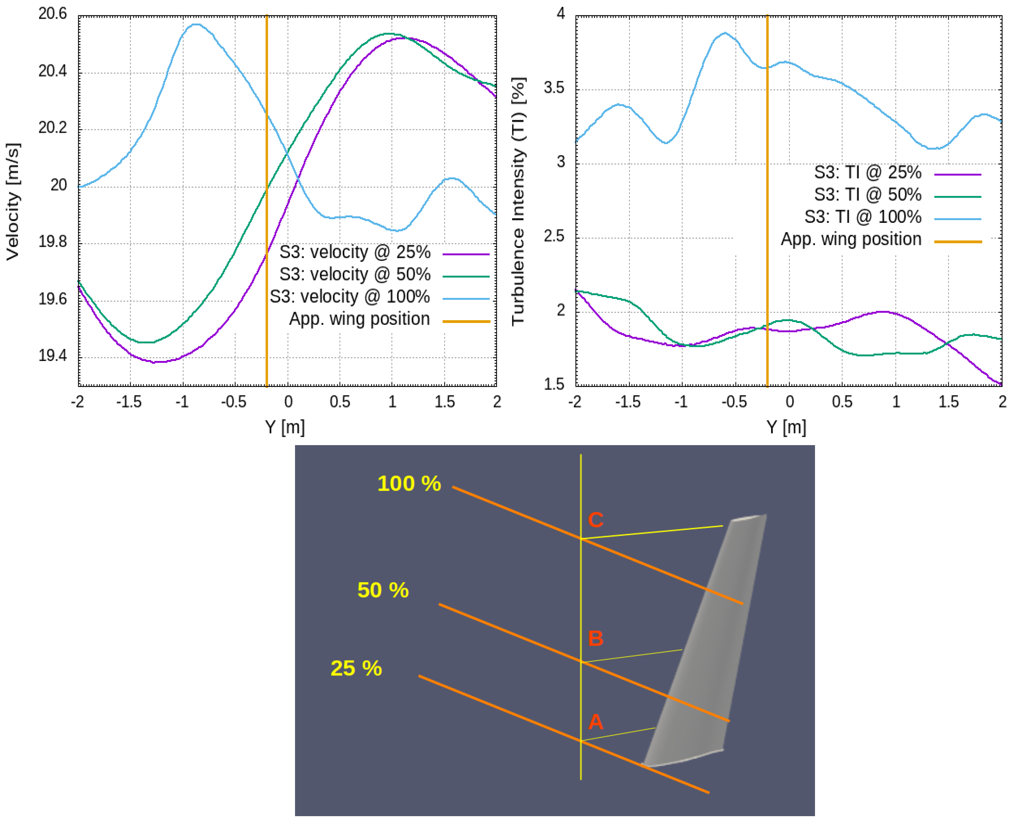
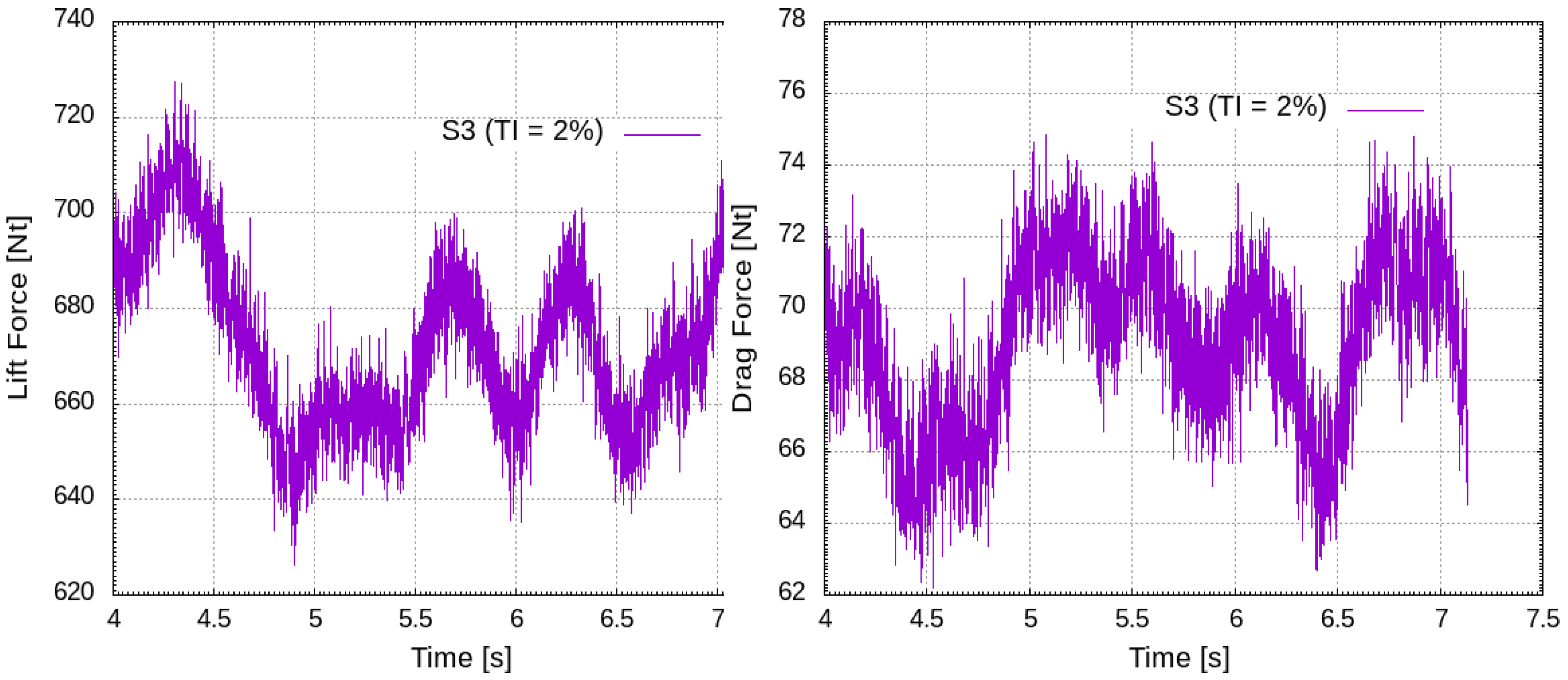
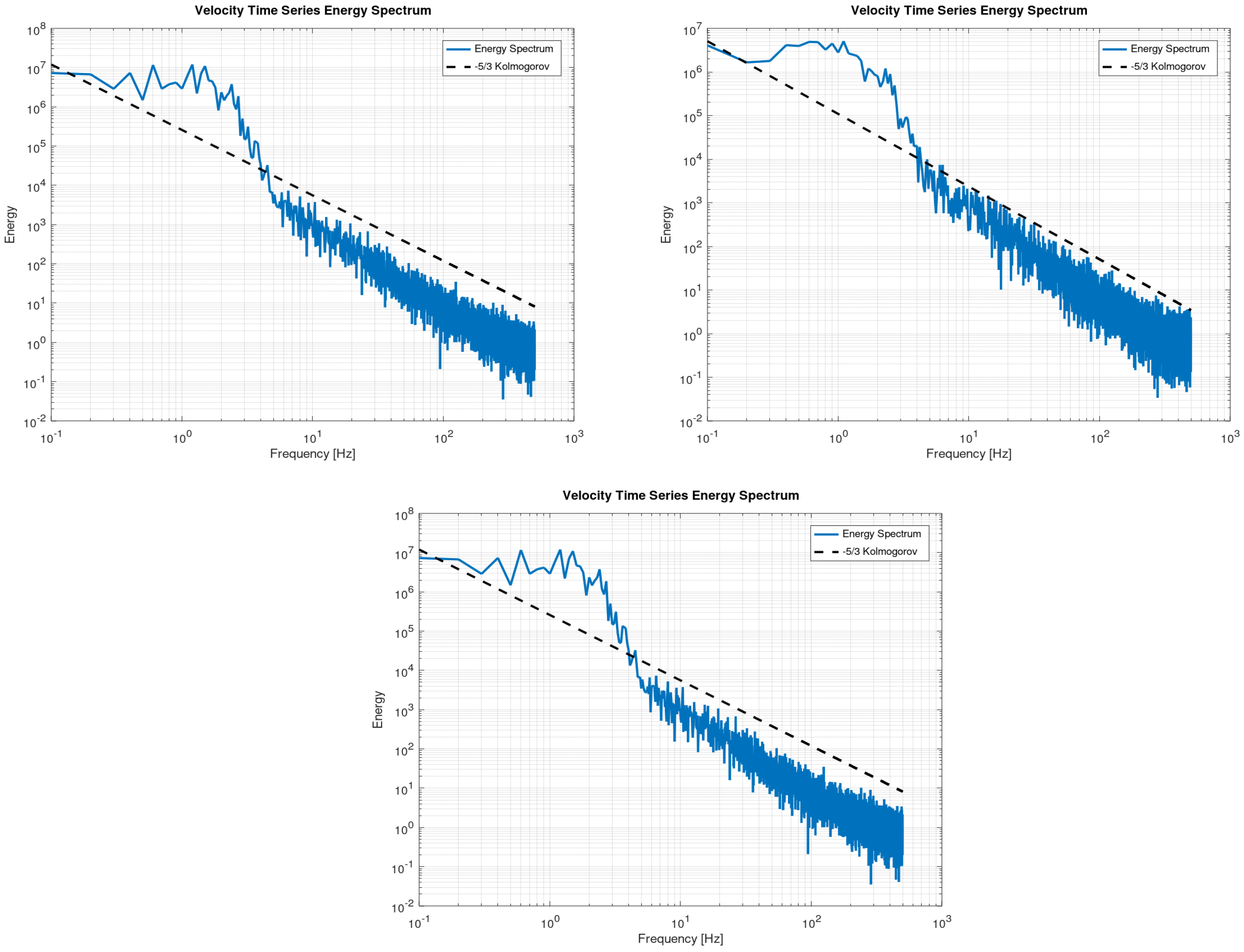
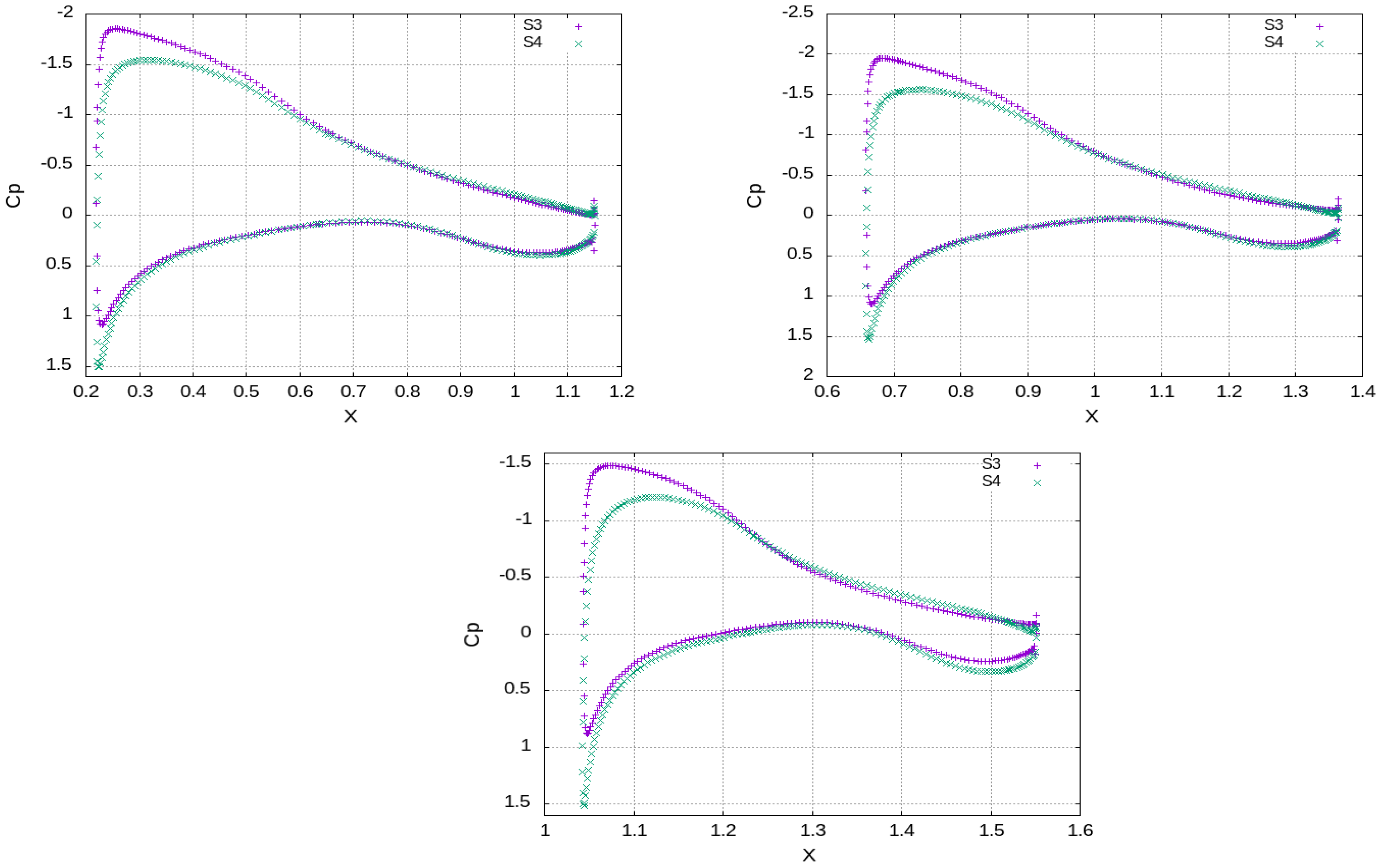
An instant of the velocity field at time t = 0.5 s, as being produced in this way, is depicted in Figure 24 where the wing has not yet encountered the incoming front. The quality of the produced velocity field is investigated through sampling the mean velocity and Reynolds stresses along the y-axis at three spanwise positions, i.e., 25 % , 50 % and 100 % of semi-span, one mean aerodynamic chord upstream of the wing; see orange lines in Figure 25. The results show that both the magnitude of the velocity field and the calculated turbulence intensity have smooth distributions spanwise. The velocity lies in the range of the freestream mean value of 20 m/s while the flow retains a considerable level of incoming turbulence, i.e., T u 2.5 % . In terms of the aerodynamic loading (see Figure 26 and Table 6), the mean value of lift reduces by approximately 10 % and the drag increases by almost 80 % in comparison to S1 case of minimal inflow turbulence. The integrity of the synthetically reproduced velocity field is also examined through a statistical analysis of the velocity time series at points A, B, C. The turbulent energy spectra (see Figure 27) follow the Kolmogorov’s law in the inertial subrange, showing a reasonable energy cascade without any spikes that would hint at high energy content of a specific eddy size. Moreover, the smooth pressure distribution on the wing, see Figure 28 also verifies the reproduction of a divergent free velocity field that ensures incompressible flow. The reduction in lift can be attributed to freestream flow irregularities that impede the normal mechanism of production of suction which reads as follows: the laminar boundary layer near the leading edge accelerates due to the curvature of the wing up to a point where a laminar separation bubble is formed, which is subsequently suppressed, and the flow reattaches as turbulent. On the contrary, the turbulent boundary layer being formed from the leading edge under the freestream turbulence conditions does not have the kinematic properties to follow this sequence; therefore, it cannot withstand the adverse pressure gradient, and it accelerates less on the wing surface, thus producing finally lower suction than the laminar one. The increase in skin friction drag is due to the large time step that impedes the prediction of laminar flow on the wing. The fact that the boundary layer is assumed to be fully turbulent is verified by the similar values of skin friction drag by cases S0 and S3 as well as by the absence of C p kinks on the S3 distribution. The increase in pressure drag can be attributed to dynamic stalls phenomena, namely the local detachment of the boundary layer due to a constantly changing AoA under a turbulent incoming flow regime. The current method is also intercompared with the stady state k ϵ turbulence model (case S4), whose inflow boundary condition for k is properly adjusted to observe the freestream turbulence intensity level. From Table 6, it is deduced that the steady state model also predicts a reduction in lift in the range of 10 % , as does C3, in comparison to S0, S1, S2, but overpredicts considerably the pressure drag. This can attributed to the effect of increased eddy vicosity, which comprises the whole content of turbulence in RANS models, on the momentum equations that result in increased acceleration of the boundary layer on the suction side. This is depicted in Figure 29 where the S4 achieves lower values than S3 of C p , which makes it evident that the flow fails to remain attached, thus producing considerable drag. This is also depicted in Figure 30 where the flow is separated in the trailing edge region and in the C p distribution where the pressure value on both pressure and suction side near the trailng edge do not coincide, which is evident of flow separation. These findings are consistent with the argument that large-scale freestream turbulence reduces the aerodynamics performance of static airfoils (Boy at al. [28], Wang and Xiao [29], Herbst et al. [30], Mahmoodilari [31]).

4. Conclusions

The current study examines the aerodynamic performance of a typical wing design for low-speed UAVs. The aim is the verification of high aerodynamic loading during the take off and landing which enables mission planning flexibility, e.g., short take off from the deck of a ship with low speed under minimal and moderate atmospheric turbulence. Special attention is paid to the WTV formation and the atmospheric conditions which are correlated to the aerodynamic loading of the aircraft under take off/landing flight conditions. The effect of the WTV and the inflow turbulence is measured with metrics such as the lift and drag while an investigation of the inception and formation of the WTV is attempted. It is worth mentioning that such numerical studies on industrial wings with taper and wash-out are very limited in the bibliography which mainly focuses on simulations with high-level turbulence modeling on wings constructed out of extrusion of standard airfoils. The main findings of the work with regards to high aerodynamic loading flight conditions read as follows:
  • The use of NLF(1)-0416 low-speed airfoil for the design of a light aircraft wing is very promising. There is strong evidence that the wing achieves significant extents of laminar flow, at least 30 % of the chord, solely through favorable pressure gradients. This results in a considerable lift-to-drag ratio close to 19 under take off/landing flight consditions (wing aerodynamic metrics: Cl = 1.147 and Cd = 0.0596 at AoA = 12 0 , which is stall condition).
  • By the flat wing tip, the boundary initially detaches at the two tip corners, and thus, two shear layers are formed which subsequently roll up and merge to form a coherent vortex. This mechanism leads to a tip vortex with significant axial velocity surplus, e.g., 1.5 × U inf , which diminishes downstream, i.e., an almost full recovery of the freestream flow is achieved at a cross-plane two chords downstream of the wing. The WTV also exhibits a straight, instead of a meandering, trajectory.
  • The CFD code delivers well in benchmarking against the wind tunnel results of the NLF airfoil at conditions AoA = 0 0 , Mach = 0.1 and Re = 1 × 10 6 . Although the kOmegaSSTLM turbulence model satisfactorily reproduces the experimental finding in 2D simulations, the IDDES model for the 3D cases around the wing is chosen since the latter does not predict but simulates the transition. In the current work, definite evidence is produced that the IDDES model can identify the transition (emergence of instabilities) even for industrial applications with relatively coarse meshes and high time steps for light aircrafts at low speeds.
  • The numerical method verifies that some shear Reynolds stresses are shifted 45 degrees from the corresponding mean strain rate in the rolling wing tip vortex, which is also verified experimentally by Chow et al. [27] and numerically by Jiang et al. [12]. This hints at the inadequacy of the Boussinesq Approximation for modeling the highly anisotropic nature of turbulence in regions such as in the vicinity of the wing tip. The calculation of Reynolds stresses through the Boussinesq assumption introduces errors that result in considerably different wake patterns. IDDES predicts a considerably higher velocity deficit and higher turbulence levels than RANS in the WTV that persist at least 3 m downstream of the wing tip. The WTV trajectory is also directed inboard (towards the empennage) while the WTV diameter widens downstream. The shadowing of the empennage (if it happens, it depends on the design) and the authority mitigation of the control surfaces is predicted to be higher by IDDES than RANS simulation. Therefore, the use of safety factors in the design of the control surfaces is recommended if the designer uses RANS models for the prediction of WTV/empennage aerodynamic interaction.
  • The inflow turbulence plays a significant role in the aerodynamic performance of the wing in question. Although the synthetically constructed velocity field that encounters the wing has a medium-level turbulence intensity T u 2 % , the predicted lift reduction is in the order of 10 % and the increase in drag close to 80 % , in comparison to minimal inflow turbulence simulation (S1). This fact does not pose a threat to the aircraft during take off, which is the main concern of the study, since a large portion of the lift is retained but increases the thrust requirements. These findings are in accordance with the bibliography that claims the aerodynamic performance mitigation of airfoils in turbulent weather calls for a more exhaustive research on the effect of turbulence on low-speed, swept-back wings under high loading conditions.
  • The wing is safe against stall at high AoA since the laminar separation bubble is suppressed, the boundary layer becomes turbulent and the flow reattaches. This is verified by the C p , C f distributions, the visualization of the flow in the bubble region and the kinematics of the flow (angles α i , ϵ ) , which are close to the theoretical values.
  • The meshing strategy, as tabulated in Table 5, gives confidence in the results which are tabulated in Table 6. All block-structured meshes (S0, S1, S2) produce high lift-to-drag ratio of about 18 to 19. S0 produces double skin friction drag vs. S1, S2 due to its fully turbulent character. S5, which is an unstructured voxel-type mesh, also identifies the transition since it produces low-level skin friction drag and a slightly higher lift than S1, S2. The voxel meshes being used for the inflow turbulence cases (S3, S4) predict both the lift reduction in comparison to minimal inflow turbulence case and the high increase in drag.

Author Contributions

Conceptualization, N.K.L., I.E.S., S.A., O.Z., P.P. and K.Y.; methodology, N.K.L.; software, N.K.L.; resources, S.A.; writing—original draft preparation, N.K.L., I.E.S., S.A., O.Z., P.P. and K.Y.; writing—review and editing, N.K.L., I.E.S., S.A., O.Z., P.P. and K.Y. All authors have read and agreed to the published version of the manuscript.

Funding

This research received no external funding.

Data Availability Statement

The original contributions presented in this study are included in the article. Further inquiries can be directed to the corresponding author.

Acknowledgments

This work was supported by computational time granted from the National Infrastructures for Research and Technology S.A. (GRNET S.A.) in the National HPC facility - ARIS - under project ID p r 016038 t h i n .

Conflicts of Interest

The authors declare no conflicts of interest.

Nomenclature

α e f f Effective Angle of Attack
α i Induced Angle of Attack
AoAAngle of Attack
ARAspect Ratio
C L Lift Coefficient
C D Drag Coefficient
DDESDelayed Deatched Eddy Simulation
ϵ Induced Downwash Angle
HPCHigh-Performance Computing
IDDESImproved Delayed Detatched Eddy simulation
kOmegaSSTLM k ω Shear Stress Transport Turbulence Model with Modeling of Transition
from Laminar to Turbulence
LESLarge Eddy Simulation
NLFNatural Laminar Flow
RANS-SAReynolds Averaged Navier–Stokes Turbulence Model of Spalart-Allmaras
URANSUnsteady Reynolds Averaged Navier–Stokes
WMLSWall-Modeled Large Eddy Simulation
WTVWing Tip Vortex
ν Kinematic viscosity

References

  1. Van Ingen, J.L. The eN method for transition prediction. Historical review of work at TU Delft. In Proceedings of the 38th Fluid Dynamics Conference and Exhibition, Seattle, DC, USA, 23–26 June 2008. [Google Scholar] [CrossRef]
  2. Langtry, R.B.; Menter, F.R. Correlation-Based Transition Modeling for Unstructured Parallelized Computational Fluid Dynamics Codes. AIAA J. 2009, 47, 2894–2906. [Google Scholar] [CrossRef]
  3. Fischer, J.S. A Framework for the Transition Delay Using Linear Stability Theory and Adjoint Optimization. Ph.D. Thesis, Universiteit Twente, Oldenburg, Germany, 1991. [Google Scholar]
  4. Spalart, P.R.; Deck, S.; Shur, M.L.; Squires, K.D.; Strelets, M.K.; Travin, A. A new version of detached-eddy simulation, resistant to ambiguous grid densities. Theor. Comput. Fluid Dyn. 2006, 20, 181–195. [Google Scholar] [CrossRef]
  5. Verhoeven, O. Trailing Edge Noise Simulations Using IDDES in OpenFOAM. Master’s Thesis, Delft University of Technology, Delft, The Netherlands, 2011. [Google Scholar]
  6. Sadraey, M.H. Aircraft Design: A System Engineering Approach; Aerospace Series; John Wiley and Sons: Chichester, UK, 2013. [Google Scholar] [CrossRef]
  7. Soltani, M.; Masdari, M.; Tirandaz, M. Effect of an end plate on surface pressure distributions of two swept wings. Chin. J. Aeronaut. 2017, 30, 1631–1643. [Google Scholar] [CrossRef]
  8. Antoniou, S.; Kapsalis, S.; Panagiotou, P.; Yakinthos, K. Parametric Investigation of Leading-Edge Slats on a Blended-Wing-Body UAV Using the Taguchi Method. Aerospace 2023, 10, 720. [Google Scholar] [CrossRef]
  9. O’Regan, M.S.; Griffin, P.C.; Young, T.M. A vorticity confinement model applied to URANS and LES simulations of a wing-tip vortex in the near-field. Int. J. Heat Fluid Flow 2016, 61, 355–365. [Google Scholar] [CrossRef]
  10. Feder, D.F.; Dhone, M.; Kornev, N.; Abdel-Maksoud, M. Comparison of different approaches tracking a wing-tip vortex. Ocean. Eng. 2018, 147, 659–675. [Google Scholar] [CrossRef]
  11. Liang, Z.; Xue, L. Detached-eddy simulation of wing-tip vortex in the near field of NACA 0015 airfoil. J. Hydrodyn. 2014, 26, 199–206. [Google Scholar] [CrossRef]
  12. Jiang, L.; Cai, J.; Liu, C. Large-eddy Simulation of Wing Tip Vortex in the Near Field. Int. J. Comput. Fluid Dyn. 2008, 22, 289–330. [Google Scholar] [CrossRef]
  13. Rogowski, K.; Hansen, M.O.L.; Hanse, R.; Piecna, J.; Lichota, P. Detached Eddy Simulation Model for the DU-91-W2-250 Airfoil. J. Phys. Conf. Ser. 2018, 1037, 022019. [Google Scholar] [CrossRef]
  14. Mitchell, A.; Morton, S.; Forsythe, J.; Cummings, R. Analysis of Delta-Wing Vortical Substructures Using Detached-Eddy Simulation. AIAA J. 2006, 44, 964–972. [Google Scholar] [CrossRef]
  15. Pereira, R.L.; Lucci, J.O.M.; Medina, F.N. Aerodynamic Performance of Natural Laminar Flow Aerofoils Applied to Low-and High-Speed Wings. In Proceedings of the 10th Aerospace Technology Congress, Stockholm, Sweden, 8–9 October 2019; Swedish Society of Aeronautics and Astronautics (FTF): Stockholm, Sweden, 2019; Available online: https://ep.liu.se/ecp/162/006/ecp19162006.pdf (accessed on 13 October 2025).
  16. Dassault Systèmes, “XFlow Brochure,” 2019. [Online]. Available online: https://www.3ds.com/ (accessed on 26 June 2019).
  17. Spalart, P.R.; Jou, W.-H.; Strelets, M.; Allmaras, S.R. Comments on the Feasibility of LES for Wings, and on a Hybrid RANS/LES. In Advances in DNS/LES; Greyden Press: Columbus, OH, USA, 1997; pp. 137–147. [Google Scholar]
  18. Shur, M.L.; Spalart, P.R.; Strelets, M.K.; Travin, A.K. A hybrid RANS-LES approach with delayed-DES and wall-modelled LES capabilities. Int. J. Heat Fluid Flow 2008, 29, 1638–1649. [Google Scholar] [CrossRef]
  19. Kim, W.W.; Menon, S. A new dynamic one-equation subgrid-scale model for large eddy simulations. In Proceedings of the 33rd Aerospace Sciences Meeting and Exhibit, Reno, NV, USA, 9–12 January 1995. [Google Scholar] [CrossRef]
  20. Poletto, R.; Craft, T.; Revell, A. A New Divergence Free Synthetic Eddy Method for the Reproduction of Inlet Flow Conditions for LES. Flow Turbul. Combust. 2013, 91, 519–539. [Google Scholar] [CrossRef]
  21. Weller, H.G.; Tabor, G.; Jasak, H.; Fureby, C. A tensorial approach to computational continuum mechanics using object-oriented techniques. Comput. Phys. 1998, 12, 620–631. [Google Scholar] [CrossRef]
  22. Somers, D.M. Design and Experimental Results for a Natural-Laminar-Flow Airfoil for General Aviation Applications; NASA Technical Paper 1861; NASA: Washington, DC, USA, 1981. [Google Scholar]
  23. Piomelli, U.; Chasnov, J.R. Large-eddy simulations: Theory and applications. In Transition and Turbulence Modelling; Henningson, D., Hallbaeck, M., Alfreddson, H., Johansson, A., Eds.; Kluwer Academic Publishers: Dordrecht, The Netherlands, 1996; pp. 269–336. [Google Scholar]
  24. Raymer, D. Aircraft Design: A Conceptual Approach, 15th ed.; American Institute of Aeronautics and Astronautics, Inc.: Reston, VA, USA, 2012. [Google Scholar] [CrossRef]
  25. McConnell, M.R.; Knight, J.; Buic, J. Improved Delayed Detached-Eddy Simulation of Turbulent Vortex Shedding in Inert Flow over a Triangular Bluff Body. Fluids 2024, 9, 246. [Google Scholar] [CrossRef]
  26. Gudmundsson, S. General Aviation Aircaft Design: Applied Methods and Procedures; Aerospace Series; John Wiley and Sons, Elsevier Science: Waltham, MA, USA, 2021; ISBN 978-0-12-818465-3. [Google Scholar]
  27. Chow, J.S.; Zilliac, G.G.; Bradshaw, P. Mean and turbulence measurements in the near field of a wingtip vortex. AIAA J. 1997, 35, 1561–1567. [Google Scholar] [CrossRef]
  28. Boy, T.E.; Djidjeli, K.; Xie, Z. Impact of Large-Scale Freestream Turbulence on a Pitching Airfoil. Flow 2023, 4, E3. [Google Scholar] [CrossRef]
  29. Wang, R.; Xiao, Z. Influence of free-stream turbulence on the aerodynamic performance of a three-dimensional airfoil. AIP Adv. 2021, 11, 075304. [Google Scholar] [CrossRef]
  30. Herbst, S.L.; Kähler, C.J.; Hain, R. Influence of large-scale free-stream turbulence on an SD7003 airfoil at low reynolds numbers. In Proceedings of the 2018 Applied Aerodynamics Conference, Atlanta, GA, USA, 25–29 June 2018. [Google Scholar]
  31. Mahmoodilari, M. The Effect of Turbulent Flow on Wind Turbine Loading and Performance. Ph.D. Thesis, University of Manchester, Manchester, UK, 2012. [Google Scholar]
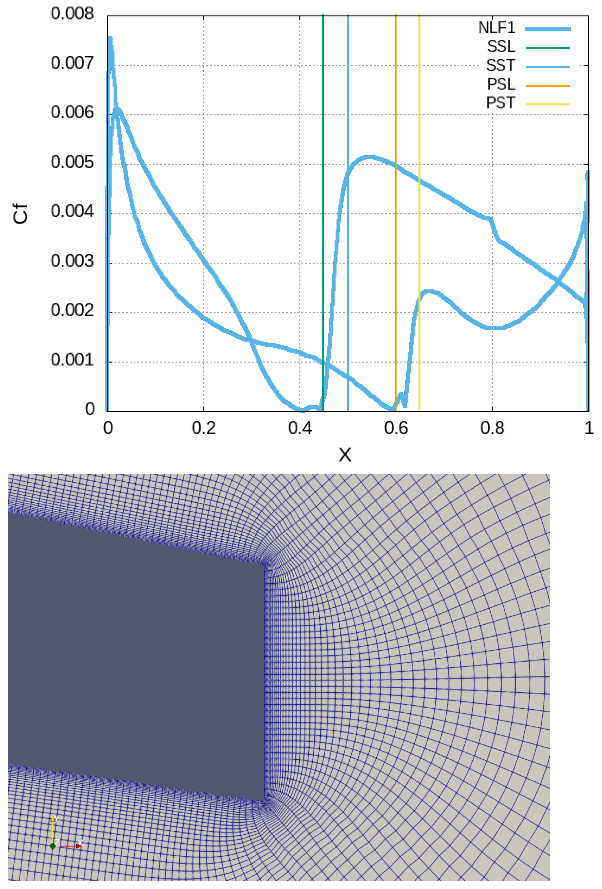
Figure 1. Cf distribution for NLF1 case (upper). Detail of the 3D computational mesh for cases NLF2, NLF3 and NLF4 in the trailing edge region (lower). The blunt trailing edge is cut-off, 0.005c wide, identical to the wind tunnel model.
Aerospace 12 00934 g001
Figure 2. Cf distribution for NLF4 case (upper, left), zoom in the transition region (upper, right) and Cp intercomparison between NLF3 and NLF4 cases (lower).
Aerospace 12 00934 g002
Figure 3. Contours of the shear stress magnitude over density [ m 2 / s 2 ] on the wing. NLF1 case, range [ 1.2 × 10 2 , 6.4 ] (left) and NLF3 range [ 3.8 × 10 4 , 6.3 ] (right).
Aerospace 12 00934 g003
Figure 4. NLF4 case. Contours of the shear stress magnitude over density [ m 2 / s 2 ] on the wing, range [ 1.8 × 10 4 , 6.5 ] (left). Q-isosurface 1 × 10 5 colored with instantaneous velocity (right).
Aerospace 12 00934 g004
Figure 5. Contours of the shear stress magnitude over density [ m 2 / s 2 ] , range [ 3.8 × 10 3 , 6.3 ] on the wing. NLF6 case (left) and NLF6 case with the surface mesh (right).
Aerospace 12 00934 g005
Figure 6. Cf distributions: NLF3 vs. NLF6 (left). NLF5 vs. NLF6 (right).
Aerospace 12 00934 g006
Figure 7. Wing design. The x-axis is aligned with the freestream direction while the y-axis points from the suction to the pressure side. The wing tapering and sweep back are recognized in the left figure while the washout in the right. The considerable aft camber of the pressure side conduces to high C l , m a x .
Aerospace 12 00934 g007
Figure 8. Type of meshes from left to right: Block-structured (left), Voxel-type (middle). Detail of the structured mesh on the wing (right).
Aerospace 12 00934 g008
Figure 9. S1 vs. S2. C p distribution (Mean) at several spanwise positions, i.e., 20 % (upper, left), 60 % (upper, right) and 95 % (lower, center) of semi-span.
Aerospace 12 00934 g009
Figure 10. S1 vs. S2. C f distribution at several spanwise positions, i.e., 20 % (upper, left), 60 % (upper, right) and 95 % (lower, center) of semi-span.
Aerospace 12 00934 g010
Figure 11. S0 vs. S5. C f distribution at several spanwise positions, i.e., 20 % (upper, left), 60 % (upper, right) and 95 % (lower, center) of semi-span.
Aerospace 12 00934 g011
Figure 12. Case S2. Isosurfaces of pressure pressure over density [ m 2 / s 2 ] , range [ 8.4 × 10 2 , 1.9 × 10 2 ] (left column) and magnitude of wall shear stress magnitude over density [ m 2 / s 2 ] , range [ 1.7 × 10 4 , 5 ] (right column, upper) and range [ 1.7 × 10 4 , 17 ] (right column, lower). Distributions on pressure side of the wing (upper figures) and suction side (lower figures).
Aerospace 12 00934 g012
Figure 13. Case S5. Isosurfaces of y + on the pressure side (left) and on the suction side (right). Non-dimensional values. Range [ 4.2 × 10 2 , 1.4 ] The spike in shear stress is evidence of transition from laminar to turbulent flow.
Aerospace 12 00934 g013
Figure 14. Case S1. Isourfaces on a plane cut at 95 % of semi-span. Metrics of pressure fluctuations over density [ m 2 / s 2 ] , range [2.5, 1900] (upper, left), DES field (0 = DDES, 1 = WMLES) (upper, right), detail of pressure fluctuation metrics over density [ m 2 / s 2 ] near the laminar separation bubble on the suction side, range [2.5, 1900] (middle, left), velocity magnitude [ m / s ] near the bubble, range [0, 32] (middle, right), variable of the turbulence model ν ˜   [ m 2 / s ] range [0, 7.7 × 10 4 ] (lower).
Aerospace 12 00934 g014
Figure 15. Streamlines emanating from 20% of span (Uz [ m / s ] range [−5, 5] ) (upper, left) and 100% of span (upper, right) (U magnitude [ m / s ] range [9.6,33]). Close-up view near the tip (Uy [ m / s ] range [–21, 21]) (lower, center).
Aerospace 12 00934 g015
Figure 16. Terminology of flow angles around the airfoil.
Aerospace 12 00934 g016
Figure 17. Effective angle of attack at 20 % (left), 60 % (right) of semi-span.
Aerospace 12 00934 g017
Figure 18. Downwash angle ϵ at 20 % (upper, left), 60 % (upper, right) and 95 % (lower, center) of semi-span.
Aerospace 12 00934 g018
Figure 19. Contours of cross-flow velocity magnitude at planes XC1 to XC6 (from left to right).
Aerospace 12 00934 g019
Figure 20. Contours of static pressure over density [ m 2 / s 2 ] at planes XC1 to XC6 (from left to right). The center of low pressure region is identified as the center of the WTV. The values of minimum pressure at each plane read as follows: XC2 (-640), XC3 (-560), XC4 (-500), XC5 (-510), XC6(-400).
Aerospace 12 00934 g020
Figure 21. Contours of axial velocity [ m / s ] in the wake core at planes XC4, XC5 and XC6 (from left to right). The values of maximum velocity read as follows: XC4 (31), XC5(28), XC6(21).
Aerospace 12 00934 g021
Figure 22. Contours of Reynolds stress v w ¯ (1st and 3rd figure) vs. mean strain rate v z + w y (2nd and 4th figure). The 1st and 2nd figure correspond to plane XC5 and the 3rd and 4th to plane XC6.
Aerospace 12 00934 g022
Figure 23. Distribution of P, U, ω n o r m across a line in the y-axis direction passing through the vortex core center at several cross-flow planes.
Aerospace 12 00934 g023
Figure 24. Case S3. Velocity field in the computational time at physical time t = 0.5 s. The x-axis is in the flow direction, the y-axis points spanwise and the z-axis is on the cross-flow plane.
Aerospace 12 00934 g024
Figure 25. Case S3. Velocity (upper, left) and turbulence intensity (upper, right) distributions along orange sampling lines at several spanwise positions (lower). The axial position of sampling points is about one mean chord upstream of the wing, while the orange lines extend about 2 mean chords laterally.
Aerospace 12 00934 g025
Figure 26. Case S3. Aerodynamic loading of the wing.
Aerospace 12 00934 g026
Figure 27. Case S3. Turbulent energy spectra at point A (upper, left), B (upper, right), C (lower, center). A, B, C points are depicted in Figure 25.
Aerospace 12 00934 g027
Figure 28. Case S1 vs. S3. Cp distribution (Mean) at several spanwise positions at 20 % (upper, left), 60 % (upper, right) and 95 % (lower, center) of semi-span.
Aerospace 12 00934 g028
Figure 29. Case S3 vs. S4. Cp distribution (Mean) at several spanwise positions at 20 % (upper, left), 60 % (upper, right) and 95 % (lower, center) of semi-span.
Aerospace 12 00934 g029
Figure 30. Case S3. Instantaneous velocity contours [ m / s ] , range [0, 31]. Macroscopic view of the the inflow turbulent field (left). Separation of the flow near the trailing edge at 60% of semi-span (right).
Aerospace 12 00934 g030
Table 1. The wing flight conditions. Cases S0, S1, S2, S3, S4, S5.
Speed [m/s]20
AoA [deg]12
Kinematic Viscosity [m2/s] 1.5 × 10 5
Density [Kg/m3]1.225
Table 2. Type of meshes and their sizes (number of points on airfoil, number of inflation layers near the wall, spanwise layers) and turbulence models used for flow simulation around the NLF airfoil. The flow conditions read as follows: Angle of Attack A o A = 0 0 , freestream velocity V = 34.3 m/s, Mach number Ma = 0.1, Re = 1 × 10 6 , ρ = 0.5215 kg/m3 and kinematic viscosity ν = 34.3 × 10 6 m2/s.
Simulation No.Type of MeshMesh Size (Cells)Turbulence Model
NLF12D320 × 100kOmegaSSTLM
NLF23D1600 × 60 × 70URANS-SA
NLF33D1600 × 60 × 70IDDES
NLF43D1600 × 60 × 70LES
NLF53D300 × 30 × 20URANS-SA
NLF63D300 × 30 × 20IDDES
Table 3. Prediction of the aerodynamic performance of the wing (lift and drag) for several combinations of turbulence models and computational meshes. The values are converged numbers for steady state simulations and arithmetic means over the sampling period for unsteady ones.
Simulation No. C l C lref C d C dref SSLSSTPSLPST
NLF10.41420.420.008560.00840.450.50.60.65
NLF20.37870.420.01270.00840.450.50.60.65
NLF30.42140.420.0070.00840.450.50.60.65
NLF40.41050.420.00750.00840.450.50.60.65
NLF50.38670.420.013110.00840.450.50.60.65
NLF60.41710.420.00730.00840.450.50.60.65
Table 4. Geometry of the wing.
Semi-Span [m]3.25
Sweep ( Λ L E ) [deg]35
Twist [deg]4
Dihedral [deg]−3
Root Chord [m]1.1
Tip Chord [m]0.5
Mean Chord [m]0.8375
Aspect Ratio (AR)8.12
Blunt trailing edge width (Tip) [mm]3.2
Blunt trailing edge width (Root) [mm]7
Table 5. Take off/landing conditions for the wing. Number of simulation, type of mesh and size of the inflation layers near the wall (points along the airfoil, number of inflation layers, number of points spanwise), turbulence model, turbulence intensity, total size of the mesh, mean y + .
NoType of MeshModel Tu ( % ) Mesh Size
(Cells)
y +
S0Block-Structured
(408 × 60 × 354)
RANS-SAMinimal32 M1
S1Block-Structured
(408 × 60 × 354)
IDDESMinimal27 M0.46
S2Block-Structured
(408 × 60 × 354)
IDDESMinimal32 M0.85
S3Voxel
(252 × 30 × 500)
IDDES≈2%13 M<1
S4Voxel
(252 × 30 × 500)
k ϵ ≈2%13 M<1
S5Voxel
(252 × 30 × 500)
IDDESMinimal17 M<1
Table 6. Prediction of the aerodynamic performance of the wing (lift and drag) for several combinations of turbulence models and computational meshes details. DR (Decay Ratio) stands for the ratio of axial to freestream velocity in the vortex core, surplus (>1) or deficit (<1), and T u for the turbulence intensity at each cross plane. The values are arithmetic means over the sampling period for unsteady simulations.
NoLift [Nt]Drag [Nt]L/DPres Drag [Nt]Visc Drag [Nt]DR (XC4) 0.5 mDR (XC6) 1.25 mDR (XC7) 3.25 mTu % (XC4) 0.5 mTu % (XC6) 1.25 mTu % (XC7) 3.25 m
S072240183460.950.840.8384.13.12
S17313819.23531.420.880.551.319.323.4
S27493819.73531.480.920.593.621.813.25
S3672699.7362.56.51------
S46441006.44928.5------
S57834218.6393------
Table 7. Estimation of α i at two spanwise positions (angle units in degrees).
Position AOA geom α eff α i
20 % 11.110.360.74
60 % 9.959.520.43
Table 8. Abbreviations used in near-wake analysis.
AbbreviationDescription
XC1Cross section at 50% of tip chord measured from the leading edge
XC2Cross section plane at 99%
XC3Cross section plane at 110%
XC4Cross section at 150%
XC5Cross section at 200%
XC6Cross section at 300%
XC7Cross section at 700%
PInstantaneous Static Pressure (P = 0 atmospheric datum pressure)
U a x i a l Instantaneous Axial Velocity
ω n o r m = ω x C t i p U inf Instantaneous normalized axial vorticity
UPrime2MeanPrime-squared mean of the velocity field
Table 9. Position of the vortex center in the wake at several cross planes.
Cross PlaneCoordinates of Vortex Center
XC3x = 1.630   y = −0.3530   z = 3.242
XC4x = 1.822   y = −0.3330   z = 3.210
XC5x = 2.065   y = −0.3260   z = 3.200
XC6x = +2.548   y = −0.3056   z = 3.176
Disclaimer/Publisher’s Note: The statements, opinions and data contained in all publications are solely those of the individual author(s) and contributor(s) and not of MDPI and/or the editor(s). MDPI and/or the editor(s) disclaim responsibility for any injury to people or property resulting from any ideas, methods, instructions or products referred to in the content.