Abstract
Agile satellites leverage rapid and flexible maneuvering to image more targets per orbital cycle, which is essential for time-sensitive emergency operations, particularly disaster assessment. Correspondingly, the increasing observation data volumes necessitate the use of on-orbit computing to bypass storage and transmission limitations. However, coordinating precedence-dependent observation, computation, and downlink operations within limited time windows presents key challenges for agile satellite service optimization. Therefore, this paper proposes a deep reinforcement learning (DRL) approach to solve the joint observation and on-orbit computation scheduling (JOOCS) problem for agile satellite constellations. First, the infrastructure under study consists of observation satellites, a GEO satellite (dedicated to computing), ground stations, and communication links interconnecting them. Next, the JOOCS problem is described using mathematical formulations, and then a partially observable Markov decision process model is established with the objective of maximizing task completion profits. Finally, we design a joint scheduling decision algorithm based on multiagent proximal policy optimization (JS-MAPPO). Concerning the policy network of agents, a problem-specific encoder–decoder architecture is developed to improve the learning efficiency of JS-MAPPO. Simulation results show that JS-MAPPO surpasses the genetic algorithm and state-of-the-art DRL methods across various problem scales while incurring lower computational costs. Compared to random scheduling, JOOCS achieves up to 82.67% higher average task profit, demonstrating enhanced operational performance in agile satellite constellations.
1. Introduction
For time-sensitive Earth observation applications in natural disaster responses, such as earthquakes, tsunamis, and floods, rapid and efficient target capture is crucial [1]. Conventional Earth Observation Satellites (CEOSs), primarily maneuverable only along the roll axis [2], are designed for systematic large-area monitoring. While effective for long-term missions, their limited agility, constrained by slower attitude control systems and fixed observation windows [3], makes them unsuitable for urgent, unpredictable scenarios. CEOSs cannot dynamically adjust their orientation during an overpass, limiting their flexibility in responding to changing mission requirements. Consequently, CEOSs struggle to provide timely and efficient coverage for critical applications, such as disaster monitoring or other time-sensitive data collection tasks, where rapid adjustment of observation windows is essential. Conversely, agile Earth Observation Satellites (AEOSs) with flexible attitude adjustment capabilities are increasingly deployed in constellations. AEOSs can capture targets before, during, and after a single overpass through rapid rotation along the roll, pitch, and yaw axes [4], effectively extending restricted observation intervals into longer observation time windows (OTWs). This capability enables AEOSs to observe affected areas at different points before, during, and after a single orbital pass by adjusting their pitch angle. As the satellite approaches the target area, it can increase its pitch angle to begin observing the region earlier, allowing for faster data acquisition, which is crucial for disaster assessment and emergency response. If the satellite has already passed over the target area, it can then decrease its pitch angle to reorient the observation, ensuring data acquisition at the earliest possible time, particularly when no other satellite is scheduled to pass over the affected area in the near future. Such flexibility is essential for mitigating damage, coordinating relief, and saving lives, as it allows for more timely data acquisition during critical emergency situations. The acquired data is subsequently downlinked to the ground, which is constrained by transmission time windows (TTWs) due to sparse ground station deployment. Hence, the agile attitude adjustment of AEOSs decouples potentially overlapping OTWs and TTWs. As illustrated in Figure 1, in the widely adopted direct ground station communication mode, CEOSs need to choose between observation and transmission during temporally overlapping windows. Due to battery constraints, we assume that observation and transmission cannot occur simultaneously in each time slot, as power limitations prevent the satellite from observing and transmitting large amounts of data at the same time. Meanwhile, AEOSs can flexibly schedule observation and transmission start times by adjusting their pitch angle, thereby enabling more target capture per orbital cycle.
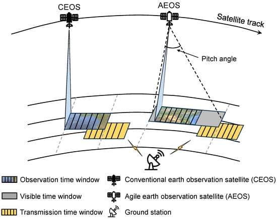
Figure 1.
A comparison of observation capabilities between CEOSs and AEOSs. The figure illustrates how AEOSs can adjust their attitude to shift the observation start time, thereby resolving the overlap between observation and transmission windows. In contrast, CEOSs can only choose one window to operate when the observation and transmission windows overlap.
Since AEOSs can have more observation opportunities within a single orbital cycle, their data acquisition volume increases accordingly, as long as operational constraints are satisfied. For instance, even if two observation objects lie along the same ground track and have overlapping observation windows, they may require different sensor configurations. One area might need higher spatial resolution, whereas the other requires a broader swath or different spectral bands. Due to limited maneuverability and fixed observation parameters, conventional CEOSs are unable to satisfy both sets of requirements within a single pass. In contrast, AEOSs can flexibly adjust their pitch angle and extend the observation window. As a result, they can start one observation before the target reaches nadir and delay the other, thereby using the appropriate imaging parameters to complete both tasks. This extended observation capability naturally generates larger volumes of data, which in turn imposes heavier burdens on onboard storage and downlink transmission, thus highlighting the necessity of adopting the on-orbit computing paradigm. Recently, more satellites have been equipped with computational units dedicated to data processing (e.g., GPU and FPGA), which enables them to process observation data locally [5,6], and transmit only essential information to ground stations, remarkably reducing downlink overhead. However, all spacecraft, including AEOSs, face inherent limitations in mass, volume, and power, which constrain the extent of their onboard computational resources. In particular, these constraints make it infeasible for AEOSs or other satellites to accommodate extensive data processing capabilities, highlighting the need for satellites that can provide computing support as processing satellites [7,8,9,10,11,12,13]. To mitigate this limitation, some constellation systems introduce specialized processing satellites, which are configured with enhanced onboard computational capacity for handling tasks offloaded from observation satellites. Such a design enables other AEOSs to strategically offload their computation tasks to processing satellites through inter-satellite links. For example, Jiang et al. [14] established satellite edge computing with high-performance computing hardware, and utilized resource allocation to achieve efficient on-orbit data processing. However, due to orbital dynamics, inter-satellite link TTWs inevitably exist, requiring that task offloading be scheduled within these windows. This constraint necessitates rational satellite mission planning and scheduling decisions. Similarly, satellite-to-ground link TTWs must also be considered when transmitting processed results to ground stations.
To achieve the efficient operation of AEOS constellations under multiple time window constraints (i.e., OTWs and TTWs), effective scheduling of observation and on-orbit computation tasks is required. Initially, substantial research efforts focused on observation scheduling for satellites [15,16], particularly for AEOSs [17,18]. Another stream of studies concentrated on data transmission scheduling [19,20], with the objective of optimizing the throughput and efficiency of the data downlink within limited TTWs. Recognizing that data acquisition is only valuable if the data can be successfully transmitted, more advanced studies have addressed the joint observation and transmission scheduling problem [21,22]. The primary goal of such joint scheduling is to resolve conflicts between OTWs and TTWs to improve end-to-end data delivery efficiency. However, existing research has not considered the on-orbit computation enabled by processing satellites. Its real-time processing capability can reduce data downlink latency, thus allowing AEOSs to complete more observation missions. Given the TTWs imposed by inter-satellite links, the rational choice between executing computational tasks locally or offloading them to processing satellites is critical for achieving efficient data processing. Hence, it is imperative to jointly consider observation scheduling and on-orbit computation scheduling.
Coordinating observation, on-orbit computation, and downlink operations in agile satellite constellations introduces a series of inherent challenges that go beyond conventional scheduling. First, the coexistence of OTWs and TTWs often leads to temporal conflicts due to power limitations, as observation and downlink operations cannot be performed simultaneously. Second, strict precedence constraints enforce that data acquisition must be completed before computation, and computation must be completed before downlink transmission, which substantially increases scheduling complexity. Third, limited on-board computational resources and constrained inter-satellite link capacity create bottlenecks when tasks are offloaded to processing satellites. Moreover, communication resource contention at both processing satellites and ground stations may cause overload if multiple transmissions occur simultaneously. Finally, these interdependent requirements substantially enlarge the decision space and increase scheduling complexity, posing significant challenges for algorithm design to balance solution quality and computational efficiency.
To overcome the above deficiencies and unsolved challenges in previous studies, we propose a joint observation and on-orbit computation scheduling (JOOCS) scheme for agile satellite constellations. The main contributions of our work are summarized as follows:
- We consider an integrated satellite-edge infrastructure comprising AEOSs, a computing-specialized processing satellite, ground stations, and cross-layer communication links. We then rigorously formulate the JOOCS problem using mathematical constraints and develop a partially observable Markov decision process (POMDP) model that optimizes task completion profit.
- We propose a novel joint scheduling algorithm based on multiagent proximal policy optimization (JS-MAPPO), a DRL algorithm, to maximize AEOS mission throughput under OTW and TTW constraints. In addition, JS-MAPPO incorporates a tailored encoder–decoder policy network that enhances learning efficiency through spatiotemporal state embedding and action masking.
- We conduct extensive simulations to validate our approach. The results demonstrate that JS-MAPPO achieves competitive performance, closely approaching the near-optimal solutions provided by the commercial solver, Gurobi, while maintaining computational efficiency. Moreover, our method outperforms other metaheuristics and DRL algorithms in terms of total task profit, especially in large-scale scenarios.
The remainder of this paper is outlined as follows. In Section 2, we provide an overview of the related work. Section 3 presents the problem formulation and the relevant POMDP model is constructed in Section 4. Section 5 elaborates on the proposed algorithm. In Section 6, we present simulation results and discussions. Finally, we give concluding remarks in Section 7.
2. Related Work
This section reviews literature relevant to scheduling optimization in agile satellite constellations. We first examine satellite observation scheduling, from single-satellite algorithms to multi-satellite coordination using machine learning and metaheuristics. Next, we analyze on-orbit computation scheduling, addressing the emergence of space-borne processing driven by increasing data volumes. Finally, we investigate existing joint scheduling frameworks, and point out the critical gap addressed by our research.
2.1. Satellite Observation Scheduling
Extensive research has investigated observation resource allocation in agile satellite networks. A comprehensive survey [2] examined AEOSs scheduling problem (AEOSSP) literature from recent decades, analyzing models, constraints, and algorithms. Early studies addressed single-satellite scenarios through metaheuristic approaches, including local search [23], hybrid differential evolution [24], and neighborhood search [25], alongside machine learning methods [26]. Recent advances incorporate deep reinforcement learning with local attention mechanisms [27], frequent pattern-based parallel search (FPBPS) algorithms [17], and bidirectional dynamic programming iterative local search (BDP-ILS) utilizing pre-computed transition times [28]. Multi-satellite coordination has gained increasing attention. Wei et al. [29] addressed multi-objective AEOSSP balancing observation profit and image quality through a multi-objective neural policy (MONP). Shang et al. [22] developed a constraint satisfaction model for energy-limited satellites, proposing the LSE-ACO-MKTA algorithm to unify observation, transmission, and charging planning. Additional studies incorporated cloud coverage impacts [30] and integrated mission scheduling [18]. Despite these advances, existing research predominantly emphasizes observation scheduling while overlooking critical transmission and computation resource coordination.
2.2. Satellite On-Orbit Computation Scheduling
The exponential growth in data volumes from advanced remote sensing cameras for Earth monitoring applications [31,32,33,34,35] has necessitated on-orbit processing to mitigate transmission bottlenecks and enable real-time operations. Mateo-García et al. [36] demonstrated a machine learning (ML) payload named “WorldFloods” on the on-orbit D-Orbit ION Satellite Carrier “Dauntless David”, which is capable of generating and transmitting compressed flood maps from observed imagery. Another study [37] deployed a lightweight foundational model named RaVAEn, a variational autoencoder (VAE), on D-Orbit’s ION SCV004 satellite. RaVAEn can generate compressed latent vectors from small image tiles, thereby enabling several downstream tasks. Building on these technological advances, researchers have developed sophisticated orbital computing solutions. Jiang et al. [38] introduced a scheduling model for complex remote sensing image processing on heterogeneous multi-processor systems (HMPS), employing directed acyclic graphs (DAGs) for parallel task representation and a Pareto-based iterative greedy optimizer (PIGO) for joint optimization. Subsequently, Jiang et al. [14] proposed SECORS, achieving substantial reductions in processing time and energy consumption through offline-online satellite operation modes and the SEC-MPH algorithm. Furthermore, an edge computing-enabled MSOCS framework [39] leveraged multiagent deep reinforcement learning (MADRL), formulating the problem as a POMDP under intermittent satellite-ground link constraints and developing a MAPPO-based solution.
2.3. Joint Scheduling
Despite increasing interest in integrated satellite mission scheduling, such research is still in its infancy. He et al. [40] analyzed coupling relationships among AEOS subsystems, developing state variable prediction methods and inference rules for different coupling states. Chatterjee et al. [41] formulated a mixed-integer nonlinear optimization model incorporating energy and memory constraints, proposing the elite mixed coding genetic algorithm (EMCGA-SS) and its hill-climbing enhanced variant (EMCHGA-SS). Assuming sufficient transmission resources, Zhu et al. [42] introduced a two-stage genetic annealing algorithm for integrated imaging and data transmission scheduling. Li et al. [43] developed an attention-based distributed satellite mission planning (ADSMP) algorithm for autonomous coordination in fully distributed AEOS constellations, addressing observation and downlink task integration.
Existing joint satellite scheduling research predominantly addresses observation–transmission coupling, while JOOCS remains largely unexplored. This paper addresses this critical gap. As on-orbit computation becomes indispensable for data-intensive missions, joint observation and computation scheduling is essential for optimizing the operational efficiency of modern agile satellite systems.
3. Problem Description
The JOOCS involves developing a collaborative scheduling strategy for the constellation of AEOSs. The primary goal is to coordinate the observation of ground targets, the on-orbit computation of collected data, and the subsequent data transmission to ground stations, all within a finite planning horizon, in order to maximize the total profit obtained from completed missions. In this problem, a set of agile satellites, denoted as , is tasked with observing a set of ground targets . Based on satellite on-orbit computing technique, the observation data can be processed locally and only the key information is transmitted to the ground, reducing downlink latency. Several available ground stations are provided to receive the data from satellites. Additionally, we consider the deployment of dedicated computing satellite with more computational resources, enabling faster on-orbit computation compared to AEOSs. Thus, AEOSs may either perform data processing locally using onboard resources (local computation) or offload computation tasks to the processing satellites (edge computation). All notations commonly used in the problem formulation are listed in Table 1.

Table 1.
Nomenclature for the JOOCS model.
The objective is to accomplish more target acquisition via scheduling observation, computation, and downlink under the constraints of OTWs and TTWs. All tasks associated with a given target execute exactly once under strict precedence constraints: computation must follow observation, and downlinking must succeed computation. Moreover, for AEOSs, the operations of observation, offloading computation to the processing satellite, and downlink exhibit mutual exclusivity, while both inter-satellite offloading and satellite-to-ground downlink transmissions are subject to communication resource constraints. We subsequently construct mathematical formulations to model this process.
- Uniqueness and Precedence Constraints: Each target m can be observed at most once during the planning horizon, i.e., it can be assigned to at most one satellite and one observation time. The constraint is formulated as follows:For any given target m, observation must be completed before subsequent actions. Computation must precede the final downlink. Then, the following constraints are established:
- Time Window Constraints: Each action must be fully executed once within a valid time window. Let denote an observation window for satellite i on target m. The observation action is constrained by the following:where denotes the indicator function, which takes the value 1 if the condition holds, and 0 otherwise. Similarly, the constraints of offloading computation to processing satellite and downlink can be formulated as follows:where indicates an available window for offloading or downlink.
- Satellite Operation Constraints: Each satellite can initiate at most one operation (observation, offloading, or downlink) at each time step t, which can be described as follows:For simplicity, we assume that on-orbit computation follows a First-In-First-Out (FIFO) queuing discipline, meaning that the computation of a task begins only after all previously arrived tasks have been executed. This assumption reduces scheduling complexity and provides a tractable framework for our study.
- Communication Resource Constraints: A constraint is imposed on the communication resources of both the processing satellite and ground stations. At any given time, each is limited to receiving a single data transmission from AEOSs, thereby preventing their communication modules from being overloaded by simultaneous transmissions. This can be formulated as follows:
4. JOOCS POMDP Model
As shown in Figure 2, the JOOCS framework consists of two components: POMDP model and MADRL. POMDP provides a formal representation of the satellite scheduling environment. This model is defined as a seven-tuple , where represents the state space, the action space, the state transition probability function, the reward function, and the observation space. denotes the reward discount factor. The value of n represents the number of agents. The second component is a MADRL approach, following the centralized training with decentralized execution (CTDE) paradigm. During the execution phase, each satellite agent (denoted as i) acts autonomously, determining its actions via a dedicated policy network () based exclusively on its local observation (). Conversely, the training phase employs a centralized critic () that leverages the global state (), an aggregation of all agent information, and generalized advantage estimation (GAE) to enable an accurate evaluation of the joint actions. The learning process is driven by an interaction loop wherein each agent selects an action upon its received observation. The environment then transitions to a new state () based on the joint action and yields a reward signal (). This reward is subsequently utilized by the MADRL to update both the individual policy networks and the centralized critic, thereby continuously optimizing the scheduling strategy.
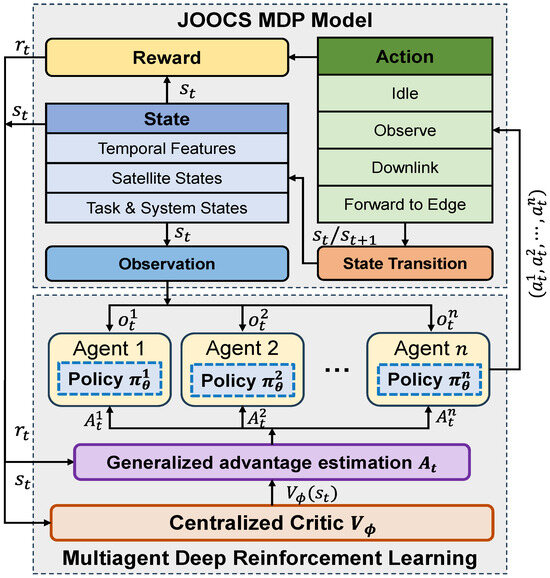
Figure 2.
The architecture of JOOCS framework.
4.1. State Space
The state at any given decision step t is represented with static and dynamic parts, which are detailed in Table 2. For the purpose of notational simplicity, the time index t is omitted from the table. The static part remains constant throughout the scheduling horizon, while the dynamic part evolves during the whole process. The total state space is formally defined as follows:
Table 2.
Dynamic feature attributes.
Specifically, the static state contains all pre-calculated time windows for potential actions, formulated as follows:
where , , and are the sets of all feasible time windows for observation, offloading, and transmission actions, respectively. The dynamic state is constructed as follows:
4.2. Observation Space
In the proposed POMDP framework, each AEOS (agent i) receives a local observation, , at any given decision step t, rather than the full global state . This local observation vector is carefully designed to provide the agent with all pertinent information required for effective decision-making, while withholding the internal states of other agents to reduce input dimensionality.
Specifically, the local observation for agent i is composed of system-wide information, its own state, and state information pertaining to all tasks. It can be formally defined as the following set:
Here, we assume that the whole system information can be obtained through multi-satellite routing mechanisms within the constellation. Since satellite system state information typically involves relatively small data volumes (e.g., task status, queue length, binary operational state), this information can be efficiently propagated through inter-satellite links with minimal bandwidth requirements. However, this approach introduces an inherent trade-off between scheduling optimality and service timeliness. While system information accessibility improves scheduling optimality, the routing process inevitably introduces communication delays that may compromise the timeliness of satellite services. This represents a limitation of our current approach, particularly in scenarios requiring low latency responses.
4.3. Action Space
The action space, , describes the set of all possible operations that can be executed by the agents at each decision step t. Within the proposed multiagent formulation, the joint action from all agents is represented as follows:
where is the action for agent i.
For an individual agent i, its is discrete and encompasses four distinct types of AEOSs operations.
- Observe: An agent selects a ground target for observation. The validity of this action is determined by whether target m is within a time window.
- Offload to Edge: An agent selects a previously observed target m to offload observation data to the processing satellite for processing. This action is constrained by the TTWs of inter-satellite link between AEOSs and the processing satellite.
- Downlink: An agent selects a previously observed and computed task related to target m to transmit the final data to an available ground station . This action is constrained by the TTWs of satellite-to-ground link.
- Idle: This serves as the default action when no other valid actions are available or selected.
At each step t, the set of available actions for each agent is dynamically determined by the environment based on the current state , considering all OTWs, TTWs, and precedence constraints. To enforce these constraints during policy execution, an action masking mechanism is employed.
The action mask is a critical mechanism that functions as a binary vector, denoted as , which has the same dimension as the action space . An element in is set to 1 if the corresponding action is valid and 0 otherwise. This mask is then applied within the actor network to filter the output logits before the final action selection. The process is as follows:
- 1.
- The actor network’s final layer outputs a vector of raw scores (logits) for every possible action.
- 2.
- The logits corresponding to all invalid actions (where the mask value in is 0) are set to a large negative number (effectively ).
- 3.
- These modified logits are then passed through a softmax function to generate the final probability distribution over the actions, where the probabilities of valid actions are normalized to sum to 1.
This procedure ensures that the probabilities for all invalid actions become zero, thereby compelling the agent to sample only from the set of currently feasible actions. This dramatically improves training efficiency and guarantees the validity of the generated schedule.
4.4. Transition Function
The state transition function determines the next state based on the current state and the joint action . In our environment, the transition is deterministic and can be expressed as . The evolution of the dynamic state is controlled by two changes:
- Action-driven Transitions: The execution of the joint action directly alters the state. The state updates for the primary actions are defined as follows.If agent i executes a successful Observe action on target m at time t, thenThis action updates the execution status of target m () to “observed”, the status of satellite i over the subsequent duration () to “busy”, and the flag indicating that target m is observed by satellite i. It also adds a new task into the local computation queue of satellite i ().If agent i executes a successful Offload action for target m at time t, thenThis action updates the execution status of target m () to “offloaded”, the status of satellite i over the subsequent duration () to “busy”, and the communication status of the processing satellite over the subsequent duration () to “busy”. It also adds a new task into the computation queue of the processing satellite.If agent i executes a successful Downlink action for target m to ground station g at time t, thenThis action updates the execution status of target m () to “transmitted”, the status of satellite i over the subsequent duration () to “busy”, the status of ground station g over the subsequent duration () to “busy”, and the flag indicating that processed result of target m (observed by satellite i) is transmitted to the ground. It also removes the corresponding task from the downlink queue of satellite i.
- Time-driven Transitions: The state also evolves implicitly with the increment of time step (). First the value of time step is normalized by . Second, upon completion of local computation for target m on satellite i, the following transitions are executed.where a task is moved from the computation queue to the downlink queue of satellite i, and the corresponding flag is updated. Finally, upon completion of edge computation for target m, the following transitions are executed.where the computation status is updated according to the length of the computation queue, and a task is moved from the computation queue to the downlink queue on the processing satellite.
4.5. Reward Function
The reward function , is defined to guide the agents toward maximizing the total profit from completed missions. A shaped reward function is employed to mitigate the issue of sparse rewards. Specifically, the total reward at each time step t is defined as a sum of rewards obtained for accomplishing a specific mission for target m, minus a constant step penalty:
where PL is a small constant penalty set to 0.01 to promote efficiency, and is the event-driven reward for task m at time t, defined as follows:
where is a fixed profit of task m. Note that, to avoid processing satellite overloading, the reward for an offload action is dynamically impacted by the length of computation queue ().
The design of the reward function in Equation (38) follows two main considerations. First, we regard a task as truly completed only when it is successfully downlinked to a ground station; therefore, in principle, the full task reward is granted at this stage. To alleviate reward sparsity during training, partial rewards are also provided at intermediate stages, namely when a task is observed and when its computation is completed. In addition, for computation offloading to the processing satellite, we introduce a dynamic reward term to discourage excessive congestion at the processing satellite and to balance the utilization of system resources. Second, the coefficients associated with these reward components were determined empirically: we conducted preliminary training runs with different candidate settings and compared their performance in terms of convergence stability and task completion profit. The final set of coefficients was chosen as the one that offered the best trade-off between training efficiency and solution quality.
5. Learning Framework and Training of JS-MAPPO
This section presents JS-MAPPO, an algorithm based on DRL. DRL is a machine learning method that is based on deep neural networks and reinforcement learning principles, and relies on foundational concepts in probability theory, statistics, and optimization. In this framework, each agile satellite is modeled as an autonomous agent that makes scheduling decisions at every time step. Based on its local observation of system status and task progress, the policy network outputs a discrete action, such as observing a target, offloading data to the processing satellite, downlinking processed results, or remaining idle. An action masking mechanism ensures that only actions satisfying time-window and precedence constraints are considered valid. Training follows the CTDE paradigm, where a centralized critic evaluates joint actions using the global state, while individual satellites execute their policies independently in real time. JS-MAPPO employs an encoder–actor–critic architecture, in which the actor network integrates two key components: a state encoder that processes high-dimensional observational data, and a recurrent neural network (RNN) module that captures temporal dependencies inherent in the scheduling sequence. Figure 3 depicts the comprehensive architecture of the proposed network.
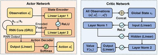
Figure 3.
The proposed encoder–actor–critic network architecture.
5.1. Actor Network
The actor network maps an agent’s local observation, , to a policy over the discrete action space. A key feature of our architecture is the state encoder, designed to handle high-dimensional and complex observation vectors efficiently. The network comprises three main components: a state encoder, an RNN core, and an action decoder.
5.1.1. State Encoder
The state encoder is implemented as a two-layer multi-layer perceptron (MLP) that extracts compact and informative feature representations from raw observation vectors. The input observation passes through a linear layer followed by a rectified linear unit (ReLU) activation, then through a second linear layer to produce the encoded feature . This transformation is formulated as follows:
where and represent the trainable parameters of the first and second linear layers, respectively.
By compressing high-dimensional and heterogeneous scheduling information into a compact embedding, the state encoder reduces input complexity and highlights task feasibility, which facilitates more stable policy learning and faster convergence.
5.1.2. RNN Core
To accommodate temporal dependencies in sequential scheduling, the encoded feature feeds into a gated recurrent unit (GRU) core. Specifically, the GRU maintains a hidden state that encodes the history of observations and actions. It employs an update gate and a reset gate to regulate information flow, allowing it to effectively capture temporal dependencies with relatively low computational complexity [44]. At each time step, the hidden state updates as follows:
where is the previous hidden state and denotes the GRU’s trainable parameters.
By capturing temporal patterns such as the opening/closing of OTWs/TTWs, queue evolution for computation/downlink, and precedence-induced state changes, the GRU yields more consistent decisions across successive time steps and improves policy stability.
5.1.3. Action Decoder
The last component of the actor network, action decoder, processes the GRU’s hidden state , which encodes both current observations and historical context. A linear layer transforms this hidden state into action logits :
where denotes the decoder’s trainable parameters. These logits parameterize the policy , with representing the complete set of actor network parameters. The policy defines a probability distribution over the discrete action space, from which action is sampled.
By combining the action decoder with an action-masking mechanism, infeasible actions that violate precedence or time-window constraints are filtered out, which reduces exploration of invalid options and improves both learning efficiency and scheduling performance.
5.2. Centralized Critic Network
The centralized critic network estimates the state-value function , providing a stable learning signal for multiple agents. Unlike the actors, the critic accesses the global state , formed by concatenating observations and relevant information from all agents. This design addresses the non-stationarity inherent in multiagent environments. The critic is implemented as an MLP with layer normalization to enhance training stability, processing the global state through sequential layers to produce a scalar value estimate.
The global state first passes through a linear layer, layer normalization, and ReLU activation to produce the hidden representation :
A second hidden layer with layer normalization and ReLU activation transforms into :
Finally, a linear output layer produces the following state-value estimate:
where , , and are the critic network’s trainable parameters, which together form the complete set of critic parameters . During training, this centralized value function estimates , which is used to compute advantage signals by comparing the observed returns with the baseline state value. These advantage estimates serve as learning signals that guide policy updates for each actor, effectively reducing the variance of the policy gradient and stabilizing the training process.
5.3. Training Algorithm
The encoder–actor–critic model is trained using the MAPPO algorithm. For brevity, we denote this MAPPO-based framework for JOOCS as JS-MAPPO. Training alternates between trajectory collection and network updates, optimizing policy and value networks using batched experience data. Algorithm 1 summarizes the JS-MAPPO procedure.
| Algorithm 1 JS-MAPPO |
|
Each training iteration computes advantage estimates via GAE to stabilize learning. The advantage for agent i at time t is as follows:
where denotes the temporal-difference (TD) error, is the discount factor, and is the GAE parameter.
In addition, the reward-to-go for agent i at timestep t is computed along each trajectory . It is defined as the discounted cumulative reward from t to the end of the trajectory:
This reward-to-go is used as training targets for the critic, in combination with GAE-based advantage estimates for updating the actor.
The critic network optimizes by minimizing the mean squared error between predictions and GAE-based targets:
where B and T denote batch size and episode length, respectively.
Actor networks update via the PPO clipped surrogate objective for stable policy improvement. The importance sampling ratio for agent i is as follows:
where denotes the current policy being optimized, and represents the previous policy used to generate the sampled trajectories. The objective function is as follows:
where is the clipping threshold, restricts the importance sampling ratio to the interval to prevent excessively large updates, and denotes the policy entropy, where the summation is taken over all valid actions after applying the action mask, weighted by to encourage exploration. Both actor and critic networks employ the Adam optimizer with gradient clipping for stability.
6. Experimental Results and Discussions
This section validates the JOOCS framework for AEOS constellations and demonstrates JS-MAPPO’s effectiveness through comparative experiments.
6.1. Simulation Scenario Setting
Experiments employed Satellite Tool Kit (STK) to generate realistic mission scenarios. Simulations initialized at 04:00:00 UTC on 6 June 2025, and span 24 h. The simulation period is discretized into 288 five-minute slots, balancing computational efficiency with scheduling flexibility. Figure 4 shows the simulation interface.
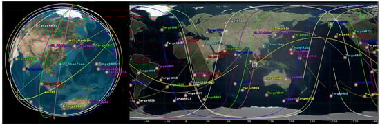
Figure 4.
STK simulation interface.
Ten AEOSs operate in the simulation, with orbital parameters derived from two-line element (TLE) data for realistic orbital dynamics. The satellites vary in inclination, altitude, and orbital plane orientation, enabling diverse coverage for task allocation. Table 3 lists the orbital parameters. Three ground stations support data reception and downlink operations: Shenzhen (22.54° N, 114.06° E), Harbin (45.80° N, 126.53° E), and Jiuquan (39.74° N, 98.52° E). Their geographic distribution across China ensures robust satellite visibility throughout orbital passes. Communication links between satellites and ground stations remain stable without disconnection throughout the simulation. Additionally, a processing satellite in geostationary orbit maintains continuous visibility with all three ground stations. The simulation includes 200 observation targets distributed across Earth’s surface. Each target has a unique identifier and geographic coordinates, with latitudes uniformly sampled from [−60°,60°] and longitudes from [−168°,168°].
Table 3.
Orbital parameters of simulated satellites.
To assess scalability and robustness across varying mission complexities, 12 simulation scenarios combine different numbers of targets and satellites. The scenarios use 3, 5, or 10 AEOSs with 50, 100, 150, or 200 observation targets. All scenarios maintain three ground stations and one geostationary processing satellite. Table 4 details each configuration.
Table 4.
Configuration of 12 simulation scenarios.
6.2. Algorithm Settings
Table 5 lists the JS-MAPPO hyperparameters. Training utilized an Intel Xeon Gold 6133 CPU with NVIDIA RTX 4090 GPU, while testing employed an Intel Core i7-11800H CPU with NVIDIA RTX 3050 Ti GPU. Training was conducted with Python 3.12.11, PyTorch 2.4.1, and NumPy 2.0.1. A total of 300 tasks were generated in advance. During training, tasks corresponding to the scale of each scenario were randomly sampled from this set, while in testing, a separate batch of tasks was sampled from the same set to ensure non-overlapping evaluation.
Table 5.
Hyperparameter settings for JS-MAPPO.
JS-MAPPO is compared against five baseline algorithms:
- (1)
- Random policy (Random) [45]: Selects feasible actions uniformly at random without using any optimization or learning mechanism, serving as a naive baseline for comparison.
- (2)
- Genetic algorithm (GA) [46]: Evolves joint action sequences using tournament selection, one-point crossover with repair, mutation, and elitist retention.
- (3)
- Counterfactual multiagent actor–critic (COMA) [47]: A multiagent RL algorithm that reduces policy gradient variance through counterfactual baselines.
- (4)
- Standard MAPPO [48]: A multiagent extension of PPO for cooperative and competitive environments.
- (5)
- Gurobi [49]: A state-of-the-art commercial optimization solver widely used for mixed-integer programming. It leverages advanced heuristics, preprocessing, and parallel computation to efficiently handle large-scale scheduling problems, and is commonly adopted as a benchmark to provide near-optimal reference solutions.
6.3. Results and Analysis
Figure 5 shows JS-MAPPO’s training curves across all 12 scenarios, with training steps on the x-axis and episodic reward on the y-axis. JS-MAPPO exhibits stable convergence across all scenarios, independent of satellite and target numbers. Scenarios with fewer targets (SCEN_1~SCEN_4) converge rapidly within steps due to lower scheduling complexity. As targets and satellites increase (SCEN_5~SCEN_12), convergence slows due to expanded action spaces and complex temporal–spatial constraints, yet performance remains high, demonstrating effective scalability. The curves show minimal post-convergence oscillations, indicating robust policies without overfitting. Notably, JS-MAPPO achieves steady improvement and high rewards even in the largest scenario (SCEN_12), demonstrating its capability for high-dimensional multiagent problems. This scalability and stability are crucial for real-time satellite constellation scheduling.
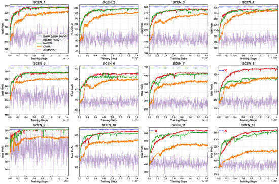
Figure 5.
Training curves of different algorithms. The red “×” mark indicates that the Gurobi solver was unable to find a solution within the specified time limit.
Table 6, Table 7 and Table 8 present performance comparisons across all scenarios using five metrics: completed tasks, completion rate, total profit, profit rate, and computational cost. JS-MAPPO consistently achieves high performance comparable to or exceeding baselines across all scales. In small-scale scenarios (SCEN_1~SCEN_4), JS-MAPPO matches Gurobi and GA performance while requiring dramatically less computation time. For example, in SCEN_3, JS-MAPPO achieves Gurobi’s completion rate (21.33%) in versus Gurobi’s . In medium-scale scenarios (SCEN_5~SCEN_8), JS-MAPPO maintains strong performance. In SCEN_7, it surpasses MAPPO in profit (417 vs. 409) and profit rate (49.58% vs. 48.63%) while computing in under . GA occasionally matches JS-MAPPO’s completion rate but requires over 2000 s, impractical for real-time applications. In large-scale scenarios (SCEN_9~SCEN_12), JS-MAPPO demonstrates excellent scalability with computation times below 1 s. In SCEN_12, it achieves the highest profit (671) and profit rate (60.23%), outperforming all baselines. Notably, Gurobi fails to produce solutions within two hours for SCEN_8, SCEN_11, and SCEN_12, highlighting its impracticality for real-time large-scale scheduling. JS-MAPPO’s stable computation times across all scales make it ideal for time-critical satellite scheduling.
Table 6.
Comparison of experimental results for SCEN_1 to SCEN_4.
Table 7.
Comparison of experimental results for SCEN_5 to SCEN_8.
Table 8.
Comparison of experimental results for SCEN_9 to SCEN_12.
In our design, the primary optimization objective of reinforcement learning training is the total profit of completed tasks, rather than the sheer number of tasks completed. As a result, there may be cases where MAPPO completes more tasks, but these tasks yield relatively low profits, leading to a lower overall return compared to JS-MAPPO. In other words, the number of completed tasks and the total profit are not strictly correlated. We included the task completion count as an additional metric mainly to provide a more intuitive illustration of scheduling behaviors. Nevertheless, when considering the actual optimization objective, JS-MAPPO consistently achieves superior overall profit.
Despite the strong performance of JS-MAPPO, several limitations remain. First, in small-scale scenarios, JS-MAPPO does not always achieve the absolute best solution quality compared with exact solvers such as Gurobi or metaheuristics such as GA. However, given its dramatically shorter computation time, this trade-off is acceptable for real-time applications. Second, the training of DRL requires substantial computational resources and a long training time, which limits its feasibility for rapid deployment. Finally, as with most DRL-based methods, the learned policies operate as black boxes and lack theoretical guarantees of optimality.
It is worth noting that in small-scale scenarios, JS-MAPPO does not always achieve the absolute best task profit compared with exact solvers such as Gurobi or metaheuristics such as GA. However, given its dramatically shorter computation time—often several orders of magnitude faster—the slight gap in solution quality is acceptable for real-time applications. In medium-scale and large-scale scenarios, JS-MAPPO shows significant advantages over exact and heuristic methods in terms of computation time, while achieving superior solution quality compared with other DRL-based approaches that operate on a similar time scale. Taken together, these results demonstrate that JS-MAPPO offers the most practical balance between effectiveness and efficiency, making it a preferable scheduling solution across different scales.
The experimental results confirm that JS-MAPPO achieves optimization-quality solutions with the computational efficiency and scalability of DRL, enabling real-time decision-making for large-scale JOOCS problems.
Figure 6, Figure 7 and Figure 8 visualize total profit and completed tasks from Table 6, Table 7 and Table 8 across different AEOSs configurations. JS-MAPPO consistently demonstrates competitive or superior performance at all scales. To assess the processing satellite’s contribution, we conducted comparative experiments on SCEN_2, SCEN_6, and SCEN_10 by removing the processing satellite. Figure 9 compares performance metrics including total profit, completed tasks, profit rate, and completion rate between configurations with and without the processing satellite. The processing satellite consistently enhances performance across all scenarios. In SCEN_2, it increases total profit and completion rate by providing accelerated task processing and additional downlink opportunities. This performance gap widens in larger scenarios (SCEN_6 and SCEN_10), where resource contention intensifies. Here, the processing satellite’s computational capacity and stable downlink links yield substantially higher profit and completion rates.
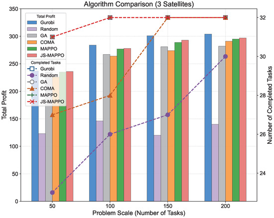
Figure 6.
Comparison of total profit and completed tasks for scenarios with 3 AEOSs.
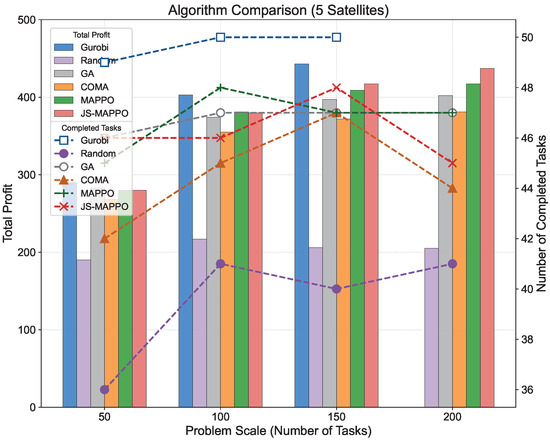
Figure 7.
Comparison of total profit and completed tasks for scenarios with 5 AEOSs.
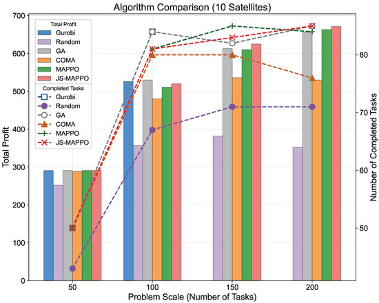
Figure 8.
Comparison of total profit and completed tasks for scenarios with 10 AEOSs.
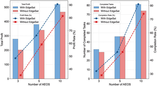
Figure 9.
Ablation study results: comparison of JS-MAPPO with and without the processing satellite.
Through analytical and empirical evaluations, we demonstrate the critical role of the processing satellite in enhancing scalability and efficiency for large-scale JOOCS problems.
7. Conclusions
In this paper, we introduced the processing satellite to alleviate the downlink pressure caused by the large volume of observation data from AEOSs, where the new challenge is how to effectively schedule observation and on-orbit computation tasks within limited time windows for achieving efficient satellite services. To solve this joint scheduling problem, we first defined the problem through mathematical formulations and established a POMDP model, before proposing a novel MADRL algorithm, JS-MAPPO. Simulation experiments across 12 scenarios demonstrate the superior performance of JS-MAPPO, which achieves up to 82.67% higher task profit than random scheduling while maintaining computational efficiency. Comparative experiments demonstrate the critical role of processing satellites in enhancing system performance under resource constraints. Our proposed JOOCS framework addresses a significant gap in satellite scheduling methodologies by jointly optimizing observation and computation decisions, enabling more efficient operations for modern AEOS constellations.
It should be acknowledged that this work gives limited consideration to the interaction between satellite attitude adjustment and scheduling, as well as the potential impact of dynamic task changes, real-time satellite resource variations, and communication delays on scheduling efficiency in practical applications. Future work could consider incorporating these factors into the model. This could specifically involve (1) incorporating real-world constraints such as energy consumption and weather impacts on observations; (2) investigating dynamic task arrival scenarios; and (3) exploring advanced solution methods to further enhance scheduling performance.
Author Contributions
Conceptualization, L.Z., Q.J., and B.C.; methodology, L.Z. and Q.J.; software, Y.Z. and L.Z.; validation, L.Z., Q.J., and Y.Z.; formal analysis, L.Z.; investigation, L.Z.; resources, B.C.; data curation, L.Z.; writing—original draft preparation, L.Z.; writing—review and editing, Q.J.; visualization, L.Z. and Q.J.; supervision, B.C.; project administration, B.C.; funding acquisition, B.C. All authors have read and agreed to the published version of the manuscript.
Funding
This research was funded by National Key Research and Development Program of China, grant number 2022YFF0503900; National Key Research and Development Program of China, grant number 2022YFD2401200; Shenzhen Higher Education Institutions Stabilization Support Program Project, grant number GXWD20220811163556003; National Natural Science Foundation of China, grant number NSFC62202127; and National Natural Science Foundation of Shenzhen, grant number JCYJ20241202123731040.
Data Availability Statement
Data are contained within the article.
Conflicts of Interest
The authors declare no conflicts of interest.
References
- Zhu, G.; Zheng, Z.; Ouyang, C.; Guo, Y.; Sun, P. An Innovative Priority-Aware Mission Planning Framework for an Agile Earth Observation Satellite. Aerospace 2025, 12, 309. [Google Scholar] [CrossRef]
- Wang, X.; Wu, G.; Xing, L.; Pedrycz, W. Agile Earth Observation Satellite Scheduling Over 20 Years: Formulations, Methods, and Future Directions. IEEE Syst. J. 2021, 15, 3881–3892. [Google Scholar] [CrossRef]
- Hahn, M.; Müller, T.; Levenhagen, J. An optimized end-to-end process for the analysis of agile earth observation satellite missions. CEAS Space J. 2014, 6, 145–154. [Google Scholar] [CrossRef]
- Lemaître, M.; Verfaillie, G.; Jouhaud, F.; Lachiver, J.M.; Bataille, N. Selecting and scheduling observations of agile satellites. Aerosp. Sci. Technol. 2002, 6, 367–381. [Google Scholar] [CrossRef]
- Giuffrida, G.; Fanucci, L.; Meoni, G.; Batič, M.; Buckley, L.; Dunne, A.; Van Dijk, C.; Esposito, M.; Hefele, J.; Vercruyssen, N.; et al. The Φ-Sat-1 mission: The first on-board deep neural network demonstrator for satellite earth observation. IEEE Trans. Geosci. Remote Sens. 2021, 60, 5517414. [Google Scholar] [CrossRef]
- Geist, A.; Crum, G.; Brewer, C.; Afanasev, D.; Sabogal, S.; Wilson, D.; Goodwill, J.; Marshall, J.; Perryman, N.; Franconi, N.; et al. NASA spacecube next-generation artificial-intelligence computing for stp-h9-scenic on iss. In Proceedings of the Small Satellite Conference, AIAA/USU, Salt Lake City, Utah, 5–10 August 2023; p. SSC23-P1-32. [Google Scholar]
- Wang, F.; Jiang, D.; Qi, S.; Qiao, C.; Shi, L. A dynamic resource scheduling scheme in edge computing satellite networks. Mob. Netw. Appl. 2021, 26, 597–608. [Google Scholar] [CrossRef]
- Leyva-Mayorga, I.; Martinez-Gost, M.; Moretti, M.; Pérez-Neira, A.; Vázquez, M.Á.; Popovski, P.; Soret, B. Satellite Edge Computing for Real-Time and Very-High Resolution Earth Observation. IEEE Trans. Commun. 2023, 71, 6180–6194. [Google Scholar] [CrossRef]
- Wen, W.; Cui, H.; He, T. Multi-Layer Reinforcement Learning Assisted Task Offloading in Satellite Edge Computing. IEEE Trans. Veh. Technol. 2025, 74, 6561–6572. [Google Scholar] [CrossRef]
- Zhou, J.; Zhao, Y.; Zhao, L.; Cai, H.; Xiao, F. Adaptive Task Offloading with Spatiotemporal Load Awareness in Satellite Edge Computing. IEEE Trans. Netw. Sci. Eng. 2024, 11, 5311–5322. [Google Scholar] [CrossRef]
- Tang, X.; Tang, Z.; Cui, S.; Jin, D.; Qiu, J. Dynamic Resource Allocation for Satellite Edge Computing: An Adaptive Reinforcement Learning-based Approach. In Proceedings of the 2023 IEEE International Conference on Satellite Computing (Satellite), Shenzhen, China, 25–26 November 2023; pp. 55–56. [Google Scholar] [CrossRef]
- Kim, J.; Kim, E.; Kwak, J. Edge Computing on the Sky: Dynamic Code Offloading Using Realistic Satellite Onboard Processors. In Proceedings of the 2024 15th International Conference on Information and Communication Technology Convergence (ICTC), Jeju, Republic of Korea, 16–18 October 2024; pp. 1818–1819. [Google Scholar] [CrossRef]
- Shi, J.; Lv, D.; Chen, T.; Li, Y. Learning-Based Inter-Satellite Computation Offloading in Satellite Edge Computing. In Proceedings of the 2024 9th International Conference on Signal and Image Processing (ICSIP), Nanjing, China, 12–14 July 2024; pp. 476–480. [Google Scholar] [CrossRef]
- Jiang, Q.; Zheng, L.; Zhou, Y.; Liu, H.; Kong, Q.; Zhang, Y.; Chen, B. Efficient On-Orbit Remote Sensing Imagery Processing via Satellite Edge Computing Resource Scheduling Optimization. IEEE Trans. Geosci. Remote Sens. 2025, 63, 1–19. [Google Scholar] [CrossRef]
- Li, J.; Li, C.; Wang, F. Automatic Scheduling for Earth Observation Satellite with Temporal Specifications. IEEE Trans. Aerosp. Electron. Syst. 2020, 56, 3162–3169. [Google Scholar] [CrossRef]
- Yang, H.; Zhang, Y.; Bai, X.; Li, S. Real-Time Satellite Constellation Scheduling for Event-Triggered Cooperative Tracking of Space Objects. IEEE Trans. Aerosp. Electron. Syst. 2024, 60, 2169–2182. [Google Scholar] [CrossRef]
- Wu, J.; Yao, F.; Song, Y.; He, L.; Lu, F.; Du, Y.; Yan, J.; Chen, Y.; Xing, L.; Ou, J. Frequent pattern-based parallel search approach for time-dependent agile earth observation satellite scheduling. Inf. Sci. 2023, 636, 118924. [Google Scholar] [CrossRef]
- Shi, Q.; Li, L.; Fang, Z.; Bi, X.; Liu, H.; Zhang, X.; Chen, W.; Yu, J. Efficient and fair PPO-based integrated scheduling method for multiple tasks of SATech-01 satellite. Chin. J. Aeronaut. 2024, 37, 417–430. [Google Scholar] [CrossRef]
- She, Y.; Li, S.; Li, Y.; Zhang, L.; Wang, S. Slew path planning of agile-satellite antenna pointing mechanism with optimal real-time data transmission performance. Aerosp. Sci. Technol. 2019, 90, 103–114. [Google Scholar] [CrossRef]
- Li, H.; Li, Y.; Liu, Y.; Deng, B.; Li, Y.; Li, X.; Zhao, S. Earth Observation Satellite Downlink Scheduling with Satellite-Ground Optical Communication Links. IEEE Trans. Aerosp. Electron. Syst. 2025, 61, 2281–2294. [Google Scholar] [CrossRef]
- He, L.; Liang, B.; Li, J.; Sheng, M. Joint Observation and Transmission Scheduling in Agile Satellite Networks. IEEE Trans. Mob. Comput. 2022, 21, 4381–4396. [Google Scholar] [CrossRef]
- Shang, M.; Yuan, R.; Song, B.; Huang, X.; Yang, B.; Li, S. Joint observation and transmission scheduling of multiple agile satellites with energy constraint using improved ACO algorithm. Acta Astronaut. 2025, 230, 92–103. [Google Scholar] [CrossRef]
- Tangpattanakul, P.; Jozefowiez, N.; Lopez, P. A multi-objective local search heuristic for scheduling Earth observations taken by an agile satellite. Eur. J. Oper. Res. 2015, 245, 542–554. [Google Scholar] [CrossRef]
- Li, G.; Chen, C.; Yao, F.; He, R.; Chen, Y. Hybrid Differential Evolution Optimisation for Earth Observation Satellite Scheduling with Time-Dependent Earliness-Tardiness Penalties. Math. Probl. Eng. 2017, 2017, 2490620. [Google Scholar] [CrossRef]
- Liu, X.; Laporte, G.; Chen, Y.; He, R. An adaptive large neighborhood search metaheuristic for agile satellite scheduling with time-dependent transition time. Comput. Oper. Res. 2017, 86, 41–53. [Google Scholar] [CrossRef]
- Lu, J.; Chen, Y.; He, R. A learning-based approach for agile satellite onboard scheduling. IEEE Access 2020, 8, 16941–16952. [Google Scholar] [CrossRef]
- Liu, Z.; Xiong, W.; Han, C.; Yu, X. Deep Reinforcement Learning with Local Attention for Single Agile Optical Satellite Scheduling Problem. Sensors 2024, 24, 6396. [Google Scholar] [CrossRef] [PubMed]
- Peng, G.; Dewil, R.; Verbeeck, C.; Gunawan, A.; Xing, L.; Vansteenwegen, P. Agile earth observation satellite scheduling: An orienteering problem with time-dependent profits and travel times. Comput. Oper. Res. 2019, 111, 84–98. [Google Scholar] [CrossRef]
- Wei, L.; Cui, Y.; Chen, M.; Wan, Q.; Xing, L. Multi-objective neural policy approach for agile earth satellite scheduling problem considering image quality. Swarm Evol. Comput. 2025, 94, 101857. [Google Scholar] [CrossRef]
- Wang, J.; Demeulemeester, E.; Hu, X.; Wu, G. Expectation and SAA Models and Algorithms for Scheduling of Multiple Earth Observation Satellites Under the Impact of Clouds. IEEE Syst. J. 2020, 14, 5451–5462. [Google Scholar] [CrossRef]
- Zhang, X.; Zhao, D.; Hu, P.; Gao, M.; Shi, Z. Optimized design of high throughput satellite antenna based on differential evolution algorithm. Chin. J. Radio Sci. 2024, 39, 1154–1159. [Google Scholar] [CrossRef]
- Qu, Q.; Liu, K.; Li, X.; Zhou, Y.; Lü, J. Satellite Observation and Data-Transmission Scheduling Using Imitation Learning Based on Mixed Integer Linear Programming. IEEE Trans. Aerosp. Electron. Syst. 2023, 59, 1989–2001. [Google Scholar] [CrossRef]
- Qin, J.; Bai, X.; Du, G.; Liu, J.; Peng, N.; Xu, M. Multisatellite Scheduling for Moving Targets Using the Enhanced Hybrid Genetic Simulated Annealing Algorithm and Observation Strip Selection. IEEE Trans. Aerosp. Electron. Syst. 2024, 60, 5773–5800. [Google Scholar] [CrossRef]
- Dakic, K.; Al Homssi, B.; Walia, S.; Al-Hourani, A. Spiking Neural Networks for Detecting Satellite Internet of Things Signals. IEEE Trans. Aerosp. Electron. Syst. 2024, 60, 1224–1238. [Google Scholar] [CrossRef]
- Lu, X.; Zhong, Y.; Zhang, L. Open-source data-driven cross-domain road detection from very high resolution remote sensing imagery. IEEE Trans. Image Process. 2022, 31, 6847–6862. [Google Scholar] [CrossRef]
- Mateo-Garcia, G.; Veitch-Michaelis, J.; Purcell, C.; Longepe, N.; Reid, S.; Anlind, A.; Bruhn, F.; Parr, J.; Mathieu, P.P. In-orbit demonstration of a re-trainable machine learning payload for processing optical imagery. Sci. Rep. 2023, 13, 10391. [Google Scholar] [CrossRef]
- Růžička, V.; Mateo-García, G.; Bridges, C.; Brunskill, C.; Purcell, C.; Longépé, N.; Markham, A. Fast Model Inference and Training On-Board of Satellites. In Proceedings of the IGARSS 2023—2023 IEEE International Geoscience and Remote Sensing Symposium, Pasadena, CA, USA, 16–21 July 2023; pp. 2002–2005. [Google Scholar] [CrossRef]
- Jiang, Q.; Wang, H.; Kong, Q.; Zhang, Y.; Chen, B. On-orbit remote sensing image processing complex task scheduling model based on heterogeneous multiprocessor. IEEE Trans. Geosci. Remote Sens. 2023, 61, 1–18. [Google Scholar] [CrossRef]
- Jiang, Q.; Han, P.; Xin, X.; Chen, K. Deep Reinforcement Learning and Edge Computing for Multisatellite On-Orbit Task Scheduling. IEEE Trans. Aerosp. Electron. Syst. 2025, 1–18. [Google Scholar] [CrossRef]
- He, C.; Dong, Y.; Li, H.; Liew, Y. Reasoning-Based Scheduling Method for Agile Earth Observation Satellite with Multi-Subsystem Coupling. Remote Sens. 2023, 15, 1577. [Google Scholar] [CrossRef]
- Chatterjee, A.; Tharmarasa, R. Reward Factor-Based Multiple Agile Satellites Scheduling with Energy and Memory Constraints. IEEE Trans. Aerosp. Electron. Syst. 2022, 58, 3090–3103. [Google Scholar] [CrossRef]
- Waiming, Z.; Xiaoxuan, H.; Wei, X.; Peng, J. A two-phase genetic annealing method for integrated earth observation satellite scheduling problems. Soft Comput. 2019, 23, 181–196. [Google Scholar] [CrossRef]
- Li, P.; Wang, H.; Zhang, Y.; Pan, R. Mission planning for distributed multiple agile Earth observing satellites by attention-based deep reinforcement learning method. Adv. Space Res. 2024, 74, 2388–2404. [Google Scholar] [CrossRef]
- Li, N.; Hu, L.; Deng, Z.L.; Su, T.; Liu, J.W. Research on GRU Neural Network Satellite Traffic Prediction Based on Transfer Learning. Wirel. Pers. Commun. 2021, 118, 815–827. [Google Scholar] [CrossRef]
- Jiang, Q.; Xin, X.; Zhang, T.; Chen, K. Energy-Efficient Task Scheduling and Resource Allocation in Edge-Heterogeneous Computing Systems Using Multiobjective Optimization. IEEE Int. Things J. 2025, 12, 36747–36764. [Google Scholar] [CrossRef]
- Zhang, J.; Xing, L. An improved genetic algorithm for the integrated satellite imaging and data transmission scheduling problem. Comput. Oper. Res. 2022, 139, 105626. [Google Scholar] [CrossRef]
- Zhang, H.; Zhao, H.; Liu, R.; Kaushik, A.; Gao, X.; Xu, S. Collaborative Task Offloading Optimization for Satellite Mobile Edge Computing Using Multi-Agent Deep Reinforcement Learning. IEEE Trans. Veh. Technol. 2024, 73, 15483–15498. [Google Scholar] [CrossRef]
- Li, Z.; Zhu, X.; Liu, C.; Song, J.; Liu, Y.; Yin, C.; Sun, W. Dynamic task scheduling optimization by rolling horizon deep reinforcement learning for distributed satellite system. Expert Syst. Appl. 2025, 289, 128350. [Google Scholar] [CrossRef]
- Seman, L.O.; Rigo, C.A.; Camponogara, E.; Bezerra, E.A.; dos Santos Coelho, L. Explainable column-generation-based genetic algorithm for knapsack-like energy aware nanosatellite task scheduling. Appl. Soft Comput. 2023, 144, 110475. [Google Scholar] [CrossRef]
Disclaimer/Publisher’s Note: The statements, opinions and data contained in all publications are solely those of the individual author(s) and contributor(s) and not of MDPI and/or the editor(s). MDPI and/or the editor(s) disclaim responsibility for any injury to people or property resulting from any ideas, methods, instructions or products referred to in the content. |
© 2025 by the authors. Licensee MDPI, Basel, Switzerland. This article is an open access article distributed under the terms and conditions of the Creative Commons Attribution (CC BY) license (https://creativecommons.org/licenses/by/4.0/).