Numerical Prediction of Fatigue Life for Landing Gear Considering the Shock Absorber Travel

Abstract

Due to the complexity of the landing gear’s (LG) structural integrity and its loads under various static or dynamic working conditions, the fatigue life assessment for LG is a highly challenging task. On the basis of the whole geometric model of a large passenger aircraft’s main landing gear (MLG), the quasi-static finite element model (FEM) of the whole MLG is established, and the high-cycle fatigue issue of the Main Fitting (MF) is studied by considering the variation in shock absorber travel (SAT). Firstly, the ground loads under actual fatigue conditions are equivalently converted into the forces acting on the center of the left and right axles of the MLG, and based on these spatial force decompositions, the magnitude and direction of the load for 12 different basic unit load cases (ULC) are obtained. That is, the stress of the MLG under actual fatigue conditions can be obtained by superimposing these ULCs. Then, considering that the SAT of the MLG varies under different fatigue conditions, and to reduce the number of finite element (FE) simulations, this article simplifies all the SAT experienced by the MLG into seven specific values, so as to establish seven quasi-static FEMs of the MLG with the specified stroke of the shock absorber. In this way, the fatigue stress of the MLG with any actual SAT can be obtained by interpolating the stress components of the seven FEMs. Only 84 FE simulations are needed to efficiently obtain the fatigue stress spectra from the ground load spectra. Finally, according to the material S-N curve and Miner’s damage accumulation criterion, evaluate the fatigue life of the Main Fitting. The results of the stress component interpolation and superposition method show that at least five different SATs of the whole MLG’s FEM are needed to effectively convert the fatigue loads into a stress spectrum. The fatigue life prediction results indicate that the minimum lifespan of the MF is 53164 landings, which means that the fatigue life meets the requirement design.

1. Introduction

As a key load-bearing device of the large passenger aircraft, landing gear (LG) supports the entire weight of the aircraft during takeoff, landing, and ground motion, and it is crucial for human–machine safety [1,2,3,4]. Especially for the main landing gear (MLG), structural fatigue is the primary failure mode during service, because it not only needs to repeatedly bear complex and heavy loads in different directions and independent changes with time but also consumes and absorbs the impact or vibration energy, such as ground impact, aircraft braking, and turning conditions [4,5,6]. Thus, when the LG is in operation, its shock absorber travel (SAT) is constantly changing [1,7,8]. To ensure the LG has sufficient load-bearing capacity, as well as the characteristics of a single-force transmission path [2], long life, and high reliability [3,4], it is generally made of high-strength alloy materials (such as 300M, 15–5PH) [1,7,9,10] with poor fatigue toughness and short crack propagation time [4,11,12]. Nowadays, an advanced civil aircraft’s LG needs to have the same lifespan as the aircraft body [13], with a service life generally ranging from 40,000 to 75,000 landings [3,14,15]. Furthermore, the EASA also explicitly states in the amendment for airworthiness regulation CS-25.571 that landing gear should adopt the safe-life design concept [16]. Obviously, the structures of LG need to undergo a large number of stress cycles during service, which belong to the problem of high-cycle fatigue (HCF). However, to design an LG that can withstand sufficient fatigue stress cycles is not an easy task.

For the design of the LG fatigue life, a full-size fatigue test is the most essential and reliable means [2,6,11,17]. The airworthiness regulations also emphasize that fatigue analysis should be supported by test evidence [15,16]. In order to more accurately evaluate the LG safety life, the fatigue test of LG usually needs to be tested in the whole aircraft [11,18,19,20]. Given that the SAT of the LG varies continuously with vertical loads during the actual takeoff and landing of the aircraft [1,7,8], the requirements for an LG fatigue test device have gradually evolved from fixed stroke to variable stroke [21,22]. However, these experiments are lengthy and costly.

Therefore, in the design phase of the LG, there is an urgent need for a method that can quickly and efficiently evaluate the fatigue life and use this method to accelerate the iteration of product design, even providing assistance for load spectrum verification and full-scale fatigue bench design. For this reason, considering the variation in SAT, an HCF assessment framework for landing gear combining a finite element method (FEM) and unit load condition is proposed.

For the HCF issues of the LG in safe-life design, in addition to the geometries and material properties of the LG components, the accurate calculation of the stress course based on load spectra is the prerequisite for fatigue damage and life prediction [3,23]. With the help of CAE technology, it is possible and effective for engineers to obtain the stress situation under complex load spectra and then calculate fatigue life through finite element (FE) simulation. Kang et al. [1] conducted a study on the fatigue life of the MLG structures based on ANSYS transient dynamics analysis and fatigue empirical formulas. Wang et al. [3] estimated the fatigue life of the MLG’s outer cylinder using the critical plane method based on FE stress results under 65 working conditions. Some articles have also reported the relevant results of using commercial FE software such as ANSYS 2022R1 to study the stress distribution patterns and the fatigue failure situation of some components of the LG [24,25,26]. Even the most popular structural optimization problems in the field of LG are focused on fatigue life in different FE models [27,28,29].It is essential to the LG’s structural integrity and the dynamic characteristics of the loads under various working conditions [30] to accurately simulate the dynamic stress response process of the landing gear during aircraft service. More recently, Chiariello et al. [7] introduced a fast dynamic stress calculation method by combining FE modal analysis and quasi-static analysis of the MLG. The above studies have investigated the fatigue life of the LG from different perspectives and greatly enriched the fatigue optimization design method for landing gear, while current studies indicate that the influence of SAT is rarely considered in predicting the fatigue life of the LG. And the asymmetry and integrity of the geometric structure are also not fully considered in the prediction model. In other words, the complex structure and numerous fatigue load conditions of the LG make life prediction very difficult.

To quickly and efficiently obtain the stress response under a large number of actual working conditions, and to elucidate the impact of SAT on the fatigue life of the LG, the technical contributions of this article are as follows: (i) Analyze the actual force transmission path of the landing gear and its unit load split technique to obtain the load coefficients. (ii) The quasi-static FEM of the whole LG is established, and the accuracy of the stress component superposition method is verified. (iii) Study the SAT simplification technique and propose a numerical prediction framework for landing gear fatigue life considering the variation in SAT.

The rest of this paper is divided into four major sections. Section 2 provides a detailed analysis of the force situation on the MLG, studies the decomposition steps of its force, and calculates the unit load coefficient. Section 3 introduces a stress component interpolation and superposition method based on quasi-static FEM to calculate the fatigue stress. Section 4 introduces SAT simplification techniques and obtains a fatigue life prediction framework with variable shock absorber travel. Section 5 discusses the impact of SAT on the stress and fatigue life of the MLG.

2. Research on Fatigue Load Decomposition

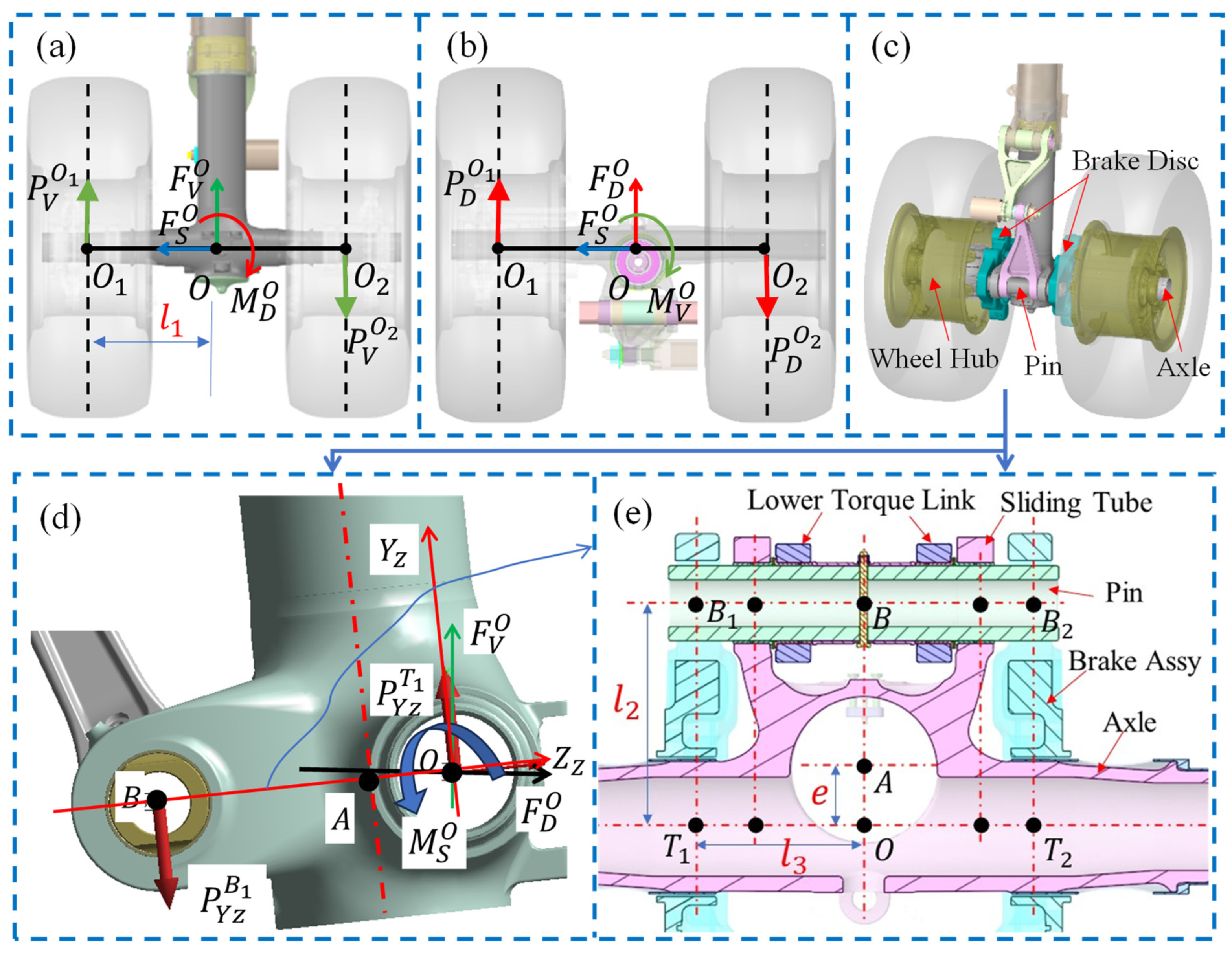
2.1. Fatigue Loads of Whole MLG 3D Model

The side view of the large passenger aircraft is shown in Figure 1a. We defined the ground inertial coordinate system (Ground-sys, DVS) as follows: the X-axis represents the opposite direction of the desired track, the vertical ground upward is the Y-axis, and the lateral Z-axis satisfies the right-hand rule. The aircraft coordinate system (Aircraft-sys, O-XYZ) is similar to the ground coordinate system, but the two coordinates differ by aircraft attitude angle, such as pitch angle. In Figure 1b, there is a certain inclination angle between the MLG Sliding Tube coordinate system (SL-sys, O-$X_z{Y}_z{Z}_z$) and the Aircraft-sys. From the angular relationship of these coordinate systems, the conversion formula for forces between Ground-sys and SL-sys are as follows:

$$\left[\begin{array}{c}{F}_{Xz}\\ F_{Yz}\\ F_{Zz}\end{array}\right]=\left[\begin{array}{ccc}\cos \theta & -\sin \theta & 0\\ \sin \theta & \cos \theta & 0\\ 0& 0& 1\end{array}\right]\times \left[\begin{array}{ccc}\cos \alpha & \sin \alpha & 0\\ -\sin \alpha & \cos \alpha & 0\\ 0& 0& 1\end{array}\right]\times \left[\begin{array}{c}{F}_D\\ F_V\\ F_S\end{array}\right]$$

(1)

where $\theta$ is the pitch angle of the aircraft and $\alpha$ is the inclination angle of MLG.

It can be seen from Figure 1c, the MLG is a partially statically indeterminate structure, and the significant structural parts are as follows: Main Fitting, Sliding Tube, Torque Links (upper and lower), Side Stay (upper and lower), and Locking Stay (upper and lower). Additional structural elements include Wheels, Axle, shock absorber, and various types of bolts, bushes, pins, etc. Among them, the Main Fitting is a statically indeterminate structure, while the Side Stay and Locking Stay are statically indeterminate structures. FWD represents the forward direction of aircraft.

There is an integrated nitrogen–oil shock absorber inside the MLG, see Figure 1c dashed box, and its oil and nitrogen phase is divided by the separation piston as shown in Figure 1d. In Figure 1d, the dashed line position of the metering pin indicates the initial uncompressed state of the shock absorber (SA). The shock absorber travel varies during the operation of the MLG. In other words, when the aircraft lands, under the action of the aircraft’s dead weight and the ground loads, the instroke of the SA is continuously compressed, and as the aircraft takes off, the outstroke of the SA slowly extends to its initial state.

During the takeoff or landing phases, the MLG that bears the excitation forces from the ground on the left Wheel is $F_{J1}$, and the right is $F_{J2}$. These forces are transmitted from the Wheels to the Axles, and then converge at the Wheel axle center point O. The load of point O can be decomposed into vertical, side, and heading force ($F_V^O$, $F_S^O$, $F_D^O$), and turning, braking, overturning moment ($M_V^O$, $M_S^O$, $M_D^O$) in the Ground-sys. Among them, vertical force is used to balance the loads of the aircraft; its transmission is from the ground to the Wheels, Axle, and then to the Sliding Tube, and then to the Main Fitting through the shock absorber. The turning moment is transmitted from the Wheel axle to the Torque Links, and then to the Main Fitting. Ultimately, the Main Fitting is connected to the Fuselage through hinge joints H1 and H2. In addition, the Main Fitting is also subjected to the force $F_{RA}$ from the Retraction actuator. The upper side Stay and Retraction actuator connect to the Fuselage through hinge joint M2 and N2.

In addition, the Retraction actuator connected to the Fuselage and the Main Fitting exerts a tensile force when the MLG is down, and a compressive force on the Main Fitting when the MLG needs to be retracted. To simplify the load, this article considers it as a constant force shown below:

$$F_{RA}=\left\{\begin{array}{l}+248 kN, \mathrm{Extension} \mathrm{status}\\ -334 kN, \mathrm{Retraction} \mathrm{status}\end{array}\right.$$

The mission profile of a large passenger aircraft during each flight includes several types of fatigue load conditions (FLCs) such as unload, tow, ground turn, breaking roll, engine run-up, takeoff roll, gear retraction and extension, landing impact, landing rollout, landing brake, etc. Each flight is divided into long range (LR), medium range (MR) and short range (SR) based on the distance traveled. Each range is composed of a series of flight types, such as A11, ~, E31, E32, E33, etc. Each flight type represents a flight spectrum, namely, a complete takeoff and landing flight mission. These flight spectrums are arranged in a specific order based on a series of FLCs mentioned above. And the FLCs included in E31 flight type are shown in

Table 1. Partial fatigue load conditions of E31 flight type in Long Range.

FLCs No.	${\mathit{F}}_{\mathit{D}}^{\mathit{O}}$ /kN	${\mathit{F}}_{\mathit{V}}^{\mathit{O}}$/kN	${\mathit{F}}_{\mathit{S}}^{\mathit{O}}$ /kN	${\mathit{M}}_{\mathit{D}}^{\mathit{O}}$ /kN·m	${\mathit{M}}_{\mathit{V}}^{\mathit{O}}$ /kN·m	${\mathit{M}}_{\mathit{S}}^{\mathit{O}}$ /kN·m	Sat /mm	$\mathit{\theta }$ /degree	k1/k2
33080302	0	226.3	0	0	0	0	320	0.18	0.5/0.5
32050501	15.9	265.2	48.3	−24.6	0	8.1	344	−0.37	0.5/0.5
32050302	21.5	358.9	−63.2	30.9	0	10.5	381	−0.41	0.5/0.5
32060223	94.7	315.8	0	14.6	−4.4	47.2	366	−0.32	0.45/0.55
32260431	0	271.2	0	−12.6	0	0	347	−0.35	0.55/0.45
32260432	67.8	271.2	0	−12.6	3.1	34.5	347	−0.36	0.5/0.5
……	……	……	……	……	……	……	……	……	……

.

2.2. Equivalent Conversion of MLG Loads

For MLG’s significant structures such as the Main Fitting, the stress at its critical location is mainly influenced by the magnitude of ground loads, but the direction of the force cannot be ignored. Generally, the stress is obtained by a finite element model (FEM) simulation, which is a prerequisite for calculating fatigue damage. In order to simulate real working conditions, the FEM of full-size MLG is established, and the actual ground loads are equivalent to aircraft wheel center points O1and O2, as shown in Figure 2 below. Considering the uneven loads between the left and right wheels, let the load distribution coefficients be k1 and k2, respectively, then

$$k_1+k_2=1$$

(2)

In Ground-sys, the overturning moment is equivalent to a pair of additional vertical forces with the same magnitude but opposite directions $P_V^{O1}$ and $P_V^{O2}$ at points O1 and O2, as shown in Figure 2a. The turning moment is equivalent to a pair of additional heading forces with the same magnitude but opposite directions $P_D^{O1}$ and $P_D^{O2}$ at points O1 and O2, as shown in Figure 2b. Thus, the actual vertical and heading force becomes

$$\left\{\begin{array}{l}{P}_V^{O1}=k_1\cdot F_V^O+M_D^O/\left(2\cdot l_1\right)\\ P_V^{O2}=k_2\cdot F_V^O-M_D^O/\left(2\cdot l_1\right)\end{array}\right.$$

(3)

$$\left\{\begin{array}{l}{P}_D^{O1}=k_1\cdot F_D^O+M_V^O/\left(2\cdot l_1\right)\\ P_D^{O2}=k_2\cdot F_D^O-M_V^O/\left(2\cdot l_1\right)\end{array}\right.$$

(4)

The side forces at points O1 and O2 only need to consider load distribution, so the conversion calculation formula is as follows:

$$\left\{\begin{array}{l}{F}_S^{O1}=k_1\cdot F_S^O\\ F_S^{O2}=k_2\cdot F_S^O\end{array}\right.$$

(5)

The aircraft Brake Assy is shown in Figure 2c. In order to simulate the actual effect of brake torque $M_S^O$, this article applies vertical force to the mounting positions of the brake disc and Axle at points T1 and T2, as well as B1 and B2 of the connecting pin shaft between the Sliding Tube and lower Torque Link, as shown in Figure 2d,e. The relationship between these forces is as follows:

$$\left\{\begin{array}{l}-F_{Yz}^{B1}=F_{Yz}^{T1}=k_1\cdot M_S^O/l_2\\ -F_{Yz}^{B2}=F_{Yz}^{T2}=k_2\cdot M_S^O/l_2\end{array}\right.$$

(6)

where the geometric model parameters involved in the above formula are given in

Table 2. MLG geometry model parameters.

Parameter	Description	Value	Unit
$sat$	Shock absorber travel	-	mm
$\theta$	Aircraft pitch angle	-	degree
$\alpha$	MLG inclination angle	5.6	degree
$e$	MLG stable spacing	58	mm
$l_1$	Half of the distance between Wheels	466	mm
$l_2$	Distance between Axle and the Pin	245	mm
$l_3$	Half of the distance between brake discs	186	mm
$l_4$	The distance of QA	1250	mm
$l_5$	Initial distance of PA	715	mm
$P_{a0}$	Initial gas pressure	2.92	MPa
$P_{atm}$	Atmospheric pressure	0.101	MPa
$V_0$	Initial gas volume	11,216,000	mm3
$n_a$	Air variability index	1.1	-
$A_a$	Pressure area	23,235	mm2

below.

By combining the above Formulas (2)–(6) and Table 1 and Table 2, the magnitude and direction of forces applied on the whole MLG model under various FLCs can be determined. Then, using Formula (1), convert these forces uniformly to the SL-sys, as shown in

Table 3. Forces of partial FLC of E31 flight type in SL-sys (kN).

Force Type	F1		F2		F3		F4				F5
FLCs No.	${\mathit{F}}_{\mathit{X}\mathit{z}}^{\mathit{O}1}$	${\mathit{F}}_{\mathit{X}\mathit{z}}^{\mathit{O}2}$	${\mathit{F}}_{\mathit{Y}\mathit{z}}^{\mathit{O}1}$	${\mathit{F}}_{\mathit{Y}\mathit{z}}^{\mathit{O}2}$	${\mathit{F}}_{\mathit{Z}\mathit{z}}^{\mathit{O}1}$	${\mathit{F}}_{\mathit{Z}\mathit{z}}^{\mathit{O}2}$	${\mathit{F}}_{\mathit{X}\mathit{z}}^{\mathit{T}1}$	${\mathit{F}}_{\mathit{X}\mathit{z}}^{\mathit{T}2}$	${\mathit{F}}_{\mathit{X}\mathit{z}}^{\mathit{B}1}$	${\mathit{F}}_{\mathit{X}\mathit{z}}^{\mathit{B}2}$	${\mathit{F}}_{\mathit{R}\mathit{A}}$
33080302	10.7	10.7	112.6	112.6	0	0	0	0	0	0	248
32050501	19	24.4	104.8	157.3	24.2	24.2	16.5	16.5	−16.5	−16.5	248
32050302	33	26	210.3	144.4	−31.6	−31.6	21.6	21.6	−21.6	−21.6	248
32060223	54	72.8	153	151.3	0	0	86.7	106	−86.7	−106	248
32260431	14.1	14.1	134.9	134.8	0	0	0	0	0	0	248
32260432	49.7	45.9	117.6	145.1	0	0	70.4	70.4	−70.4	−70.4	248
……	……	……	……	……	……	……	……	……	……	……	……

below:

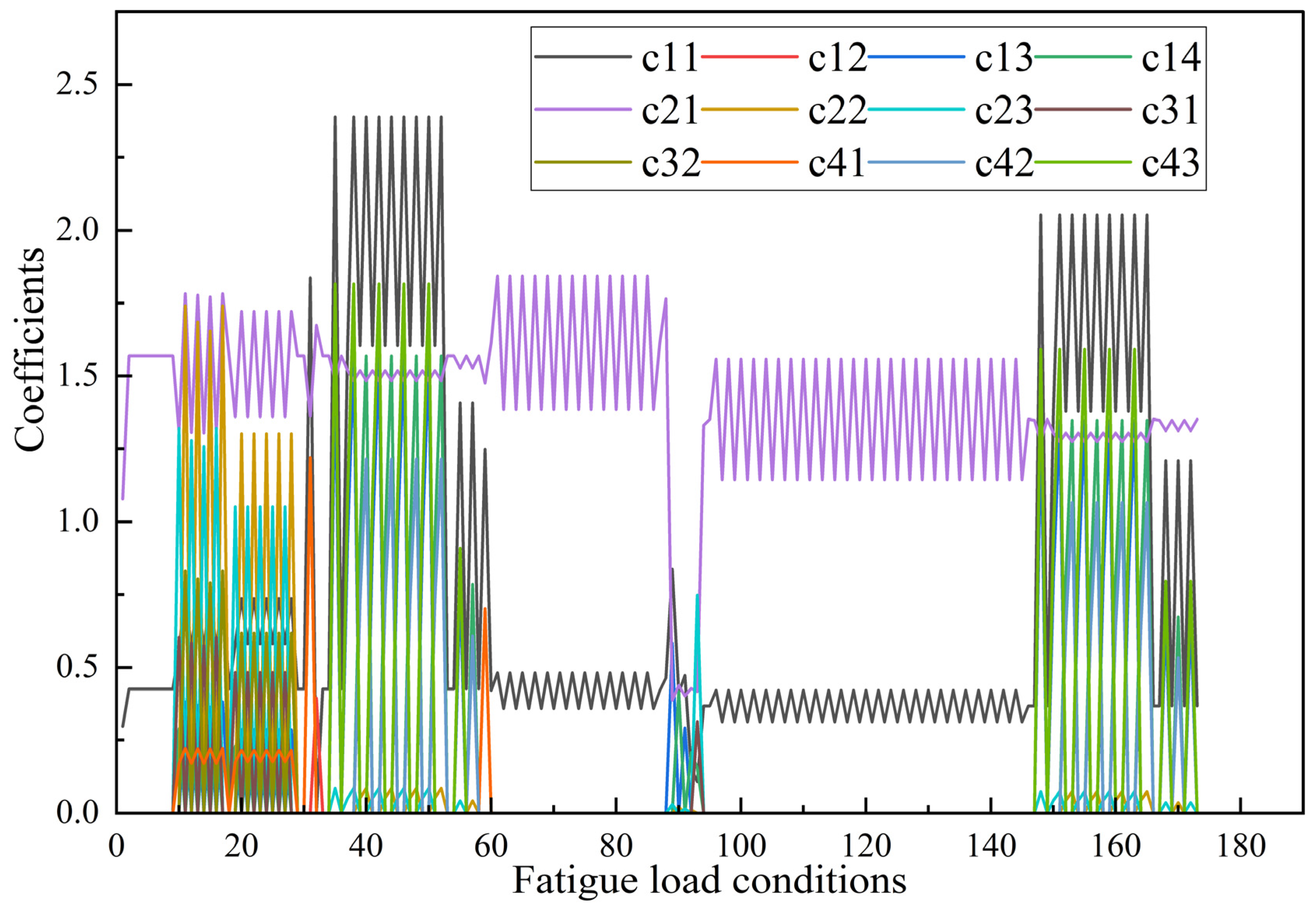
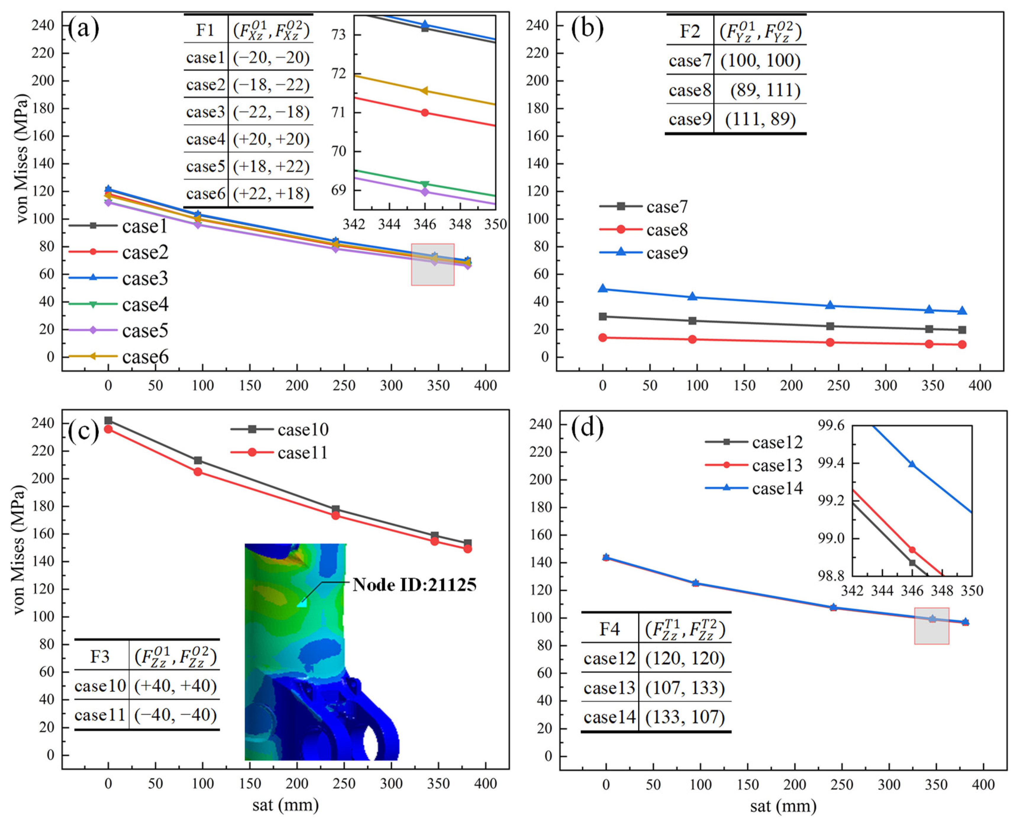
2.3. Load Coefficients for Unit Load Case

According to the previous analysis of the loads equivalent conversion of the whole 3D model, as shown in Figure 1c and Table 3, the external forces of MLG can be divided into five types. That is, the heading, vertical, and side forces acting on the left and right wheel center points O1 and O2; the vertical forces on the points T1, T2, B1, and B2 to simulate the effect of the brake torque $M_S^O$ of Wheels; and the force $F_{RA}$ exerted by the Retraction actuator. In order to reduce finite element simulations, and based on the characteristics of Table 3 forces above, this paper uses unit load cases (ULCs) in following

Table 4. Force values of unit load cases (kN).

Force Location	Unit Load Values	$\mathbf{Unit} \mathbf{Load} \mathbf{Types} {\mathit{P}}_{\mathit{u}\mathit{v}}$	Location of Force Application
$\left(F_{Xz}^{O1},F_{Xz}^{O2}\right)$	(+40,+40); (−40,−40); (+10,−10); (−10,+10)	$P_{11}~P_{14}$	Heading force of O1 and O2, other forces set to 0
$\left(F_{Yz}^{O1},F_{Yz}^{O2}\right)$	(+100,+100); (+20,−20); (−20,+20)	$P_{21}~P_{23}$	Vertical force of O1 and O2, other forces set to 0
$\left(F_{Zz}^{O1},F_{Zz}^{O2}\right)$	(+40,+40); (−40,−40)	$P_{31}~P_{32}$	Side force of O1 and O2, other forces set to 0
$\left(F_{Zz}^{\mathrm{T}1},F_{Zz}^{\mathrm{T}2}\right)$	(+100,+100); (100,122); (122,100)	$P_{41}~P_{43}$	Vertical force of T1, T2, and B1, B2 obtained from formula(6)
$F_{RA}$	+248; −334	$P_{51}~P_{52}$	Point M1, other forces set to 0

to further simplify fatigue conditions.

Based on the superposition property of forces, for any type of force of an FLC in Table 3, such as a heading force, at most invokes two ULCs of the same type force in Table 4 for superposition. Therefore, each FLC is formed by superimposing several ULCs, and the formula is as follows:

$$F_u={\displaystyle {\sum }_v{c}_{uv}\cdot P_{uv}}$$

(7)

where $c_{uv}$ are the load coefficients of ULCs and need to satisfy $c_{uv}$ ≥ 0, $u$ = 1–5 represents the external load type and $v$ = 1–4 represents the unit load type as shown in Table 4.

Therefore, the ground load under actual fatigue conditions is equivalently converted into the forces acting on the center of the left and right axles of the MLG. According to the spatial forces system decomposition, it can be known that the load experienced by any fatigue condition can be obtained by superimposing 12 ULCs and their load coefficients. That is to say, for any actual fatigue condition, it can be obtained by superimposing 14 basic unit load conditions; see Table 4 mentioned above. In summary, obtain the coefficients for each FLC through the following steps:

Step 1: Perform a force analysis of the whole MLG 3D-model (Figure 1), and compile a fatigue load spectrum (Table 1);

Step 2: According to Formulas (2)–(6), carry out an equivalent conversion of loads;

Step 3: Using Formula (1), convert forces uniformly to the SL-sys;

Step 4: Calculate the load coefficients of ULCs by Formula (7) and Table 4;

Step 5: Return to step 1, until all flight types are considered.

For the LR consisting of 12,000 flight types, take its E31 flight type as an example; the partial coefficients of the ULC calculated from the above steps are shown in Figure 3.

3. Stress Component Superposition Method

3.1. Quasi-Static Finite Element Modeling

According to the stroke of the SA corresponding to actual fatigue conditions (see Table 1), complete the assembly of the MLG 3D solid model in SpaceClaim 2022R1 software. Subsequently, import it into ANSYS/Workbench 2022R1 software to establish an overall FEM, consisting of 767,960 elements (SOLID186) and 1,365,958 nodes. Among them, the Main Fitting has 150,706 elements (SOLID186) and 27,1596 nodes.

For the boundary conditions of FEM, considering the load transmission path of ground loads, the pins connected to the Fuselage are constrained by the multi-point coupling elements (MPC184) [1,3,7], as shown in Figure 4a.

Moreover, considering the motions and constraints relationship of each structure, all the components that contact the Main Fitting are set to friction contact, and these element types are TARGE170 and CONTA174, respectively. In this way, the FEM in this paper is contact nonlinear; see Figure 4b,c.

During the takeoff and landing process of the aircraft, the nitrogen–oil shock absorber is continuously compressed to absorb and disperse ground impact forces, which is similar to the action of springs and damping [5,8,30]. In order to simulate the vertical force transmission effect of the SA, a spring element (Combin14) is used in the FEM, as shown in Figure 4b. Specifically, the relationship between vertical load $F_V^O$ and SAT is determined by the air spring force $F_a$ and the oil damping force $F_d$ of the SA as the following formula:

$$F_V^O=F_a+F_d$$

(8)

In our previous article [8], the air spring force $F_a$ is expressed as

$$F_a=\left(P_{a0}{\left({\displaystyle \frac{V_0}{V_0-A_a\cdot sat}}\right)}^{n_a}-P_{atm}\right)A_a$$

(9)

where $P_{a0}$ represents the initial gas pressure, $P_{atm}$ designates the atmospheric pressure, $V_0$ is the initial gas volume of the shock absorber, $A_a$ represents the pressure area the Sliding Tube, $n_a$ is the air variability index, and $sat$ is the stroke of the shock absorber. The data of the above MLG shock absorber are shown in Table 2.

In the quasi-static model, the oil damping force $F_d$ can be neglected due to the small changes in SAT. Therefore, as shown in Figure 4b, the stiffness of the spring element in the FEM under any SAT can be known by taking the derivative of Formula (8) and combining Formula (9). Moreover, as shown in Figure 4d, the oil and gas pressure $P_a$ and $P_b$ inside the SA can be obtained as follows:

$$P_a=P_b=F_V^O/A_a$$

(10)

From this, it can be seen that the FEM of the MLG in this article is also geometrically nonlinear. Taking fatigue load condition No. = 32050302 in Table 3 as an example, the load applied in the full-size FEM is shown in Figure 4e. Substituting the known parameters of this condition, when sat = 381 mm, the stiffness of the spring element is $K$ = $4.07\times {10}^6$ N/mm, and the pressure is $P_a$ = $P_b$ = 16.1 MPa (see Figure 4d). Then, the stress cloud diagram after finite element simulation is shown in Figure 4f.

Figure 4 shows the steps of obtaining stress through quasi-static FEM for a specific fatigue condition. Similarly, the direct FE simulation method for any other fatigue condition is similar. But using direct FE simulation for a large number of similar fatigue conditions is very time-consuming. To this end, we introduce a method of using stress component interpolation and superposition, with the following specific steps:

Step 1: Establish a quasi-static FEM for the whole 3D model of the LG (where SAT is the initial value) using the method shown in Figure 4.

Step 2: Analyze the SAT distribution of all fatigue load conditions and select several representative SATs. Here, 7 SATs have been selected, as detailed in Section 4.1.

Step 3: Adjust the SAT of the 3D model of the LG to sat1, apply a unit load (see Table 3), and obtain the stress response under unit load conditions according to Step 1. Similarly, the other 6 SATs are similar.

Step 4: Calculate the load coefficients for any actual fatigue load condition using the formulas in Section 2.3.

Step 5: Based on the stress situation of Step 3 and the load coefficients of Step 4, the stress component interpolation superposition method is used to calculate the stress of this actual fatigue condition. The specific derivation is shown in Section 4.2.

The illustration of the above steps is shown in Section 4.

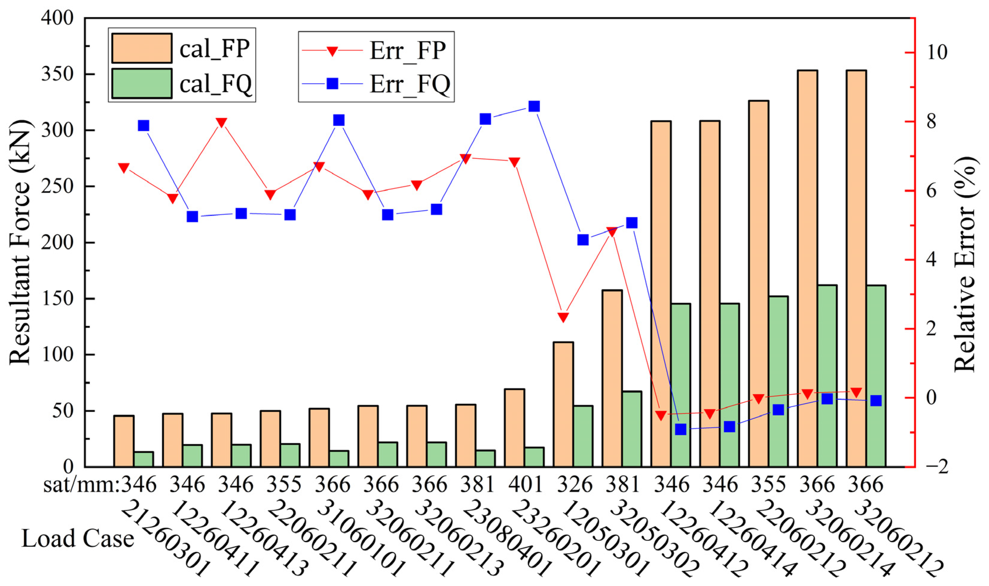
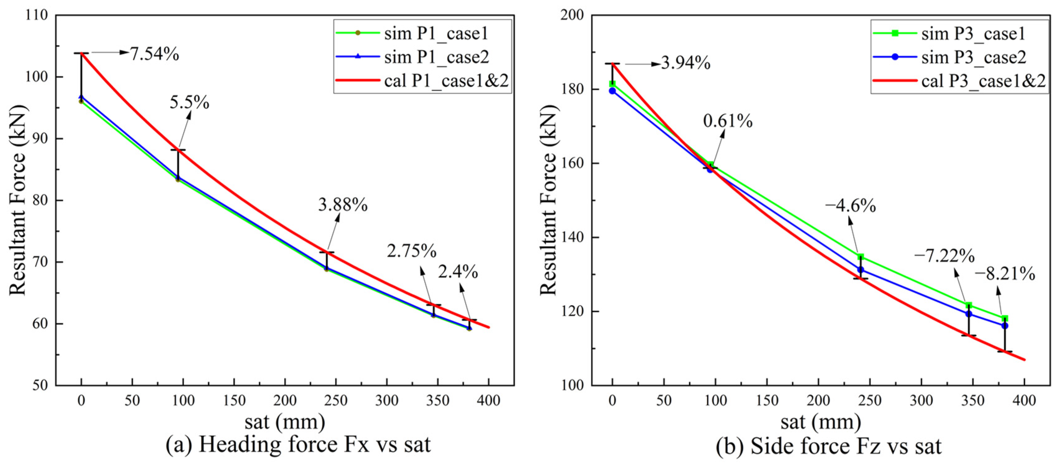
3.2. FEM Internal Force Validation

This article verifies the FEM in Figure 4 by comparing the simulated and theoretical values of force. The structures of the shock absorber are shown in Figure 1d; then list the force balance equations of position Q as follows:

$$\left\{\begin{array}{l}{F}_{Xz}^A+F_{Xz}^P+F_{Xz}^Q=0\\ F_{Zz}^A+F_{Zz}^P+F_{Zz}^Q=0\\ M_{Xz}^A+F_{Zz}^P\cdot \left(l_5-sat\right)+F_{Zz}^Q\cdot l_4=0\\ M_{Zz}^A-F_{Xz}^P\cdot \left(l_5-sat\right)-F_{Xz}^Q\cdot l_4=0\end{array}\right.$$

(11)

where $l_4$ and $l_5$ are taken from Table 2, and the load of point A is calculated from the load of point O as follows:

$$\left\{\begin{array}{l}\left[\begin{array}{l}{F}_{Xz}^A\\ F_{Yz}^A\\ F_{Zz}^A\end{array}\right]=\left[\begin{array}{l}{F}_{Xz}^O\\ F_{Yz}^O\\ F_{Zz}^O\end{array}\right]\\ \left[\begin{array}{l}{M}_{Xz}^A\\ M_{Yz}^A\\ M_{Zz}^A\end{array}\right]=\left[\begin{array}{l}{M}_{Xz}^O\\ M_{Yz}^O\\ M_{Zz}^O\end{array}\right]+\left[\begin{array}{ccc}0& 0& 0\\ 0& 0& -e\\ 0& e& 0\end{array}\right]\left[\begin{array}{l}{F}_{Xz}^O\\ F_{Yz}^O\\ F_{Zz}^O\end{array}\right]\end{array}\right.$$

(12)

Combining Equations (13) and (14), the forces of P are derived as follows:

$$\left\{\begin{array}{l}{F}_{Xz}^P=-{\displaystyle \frac{M_{Zz}^O+e\cdot F_{Zz}^O+F_{Xz}^O\cdot l_4}{l_4-l_5+sat}}\\ F_{Zz}^P={\displaystyle \frac{M_{Xz}^O-F_{Zz}^O\cdot l_4}{l_4-l_5+sat}}\end{array}\right.$$

(13)

Then, considering the friction situation of position P, with a friction coefficient of ${\mu }_P$ = 0.05, the vertical force is as follows:

$$F_{Yz}^P={\mu }_P\cdot \sqrt{{\left(F_{Xz}^P\right)}^2+{\left(F_{Zz}^P\right)}^2}$$

(14)

Similarly, the forces of position Q can be calculated.

Subsequently, randomly select 16 fatigue conditions from Table 1, and calculate the resultant force on the point of P and Q using Formulas (13) and (14), shown as $cal\_F_P$ and $cal\_F_Q$ in Figure 5. Extract the loads of these 16 fatigue conditions from Table 3 and perform FE simulation with reference to Figure 4. Thus, the contact reaction force of the target surfaces of the positions P and Q, denoted as $sim\_F_P$ and $sim\_F_Q$, can be obtained by FE simulation. The forces relative error of theoretically calculated and direct FE simulation is shown in Figure 5.

It can be seen from Figure 5 that the maximum relative error of joint force between the FE simulated and the theoretical calculation value is 8.45%, which indicates that the FEM shown in Figure 4 is correct.

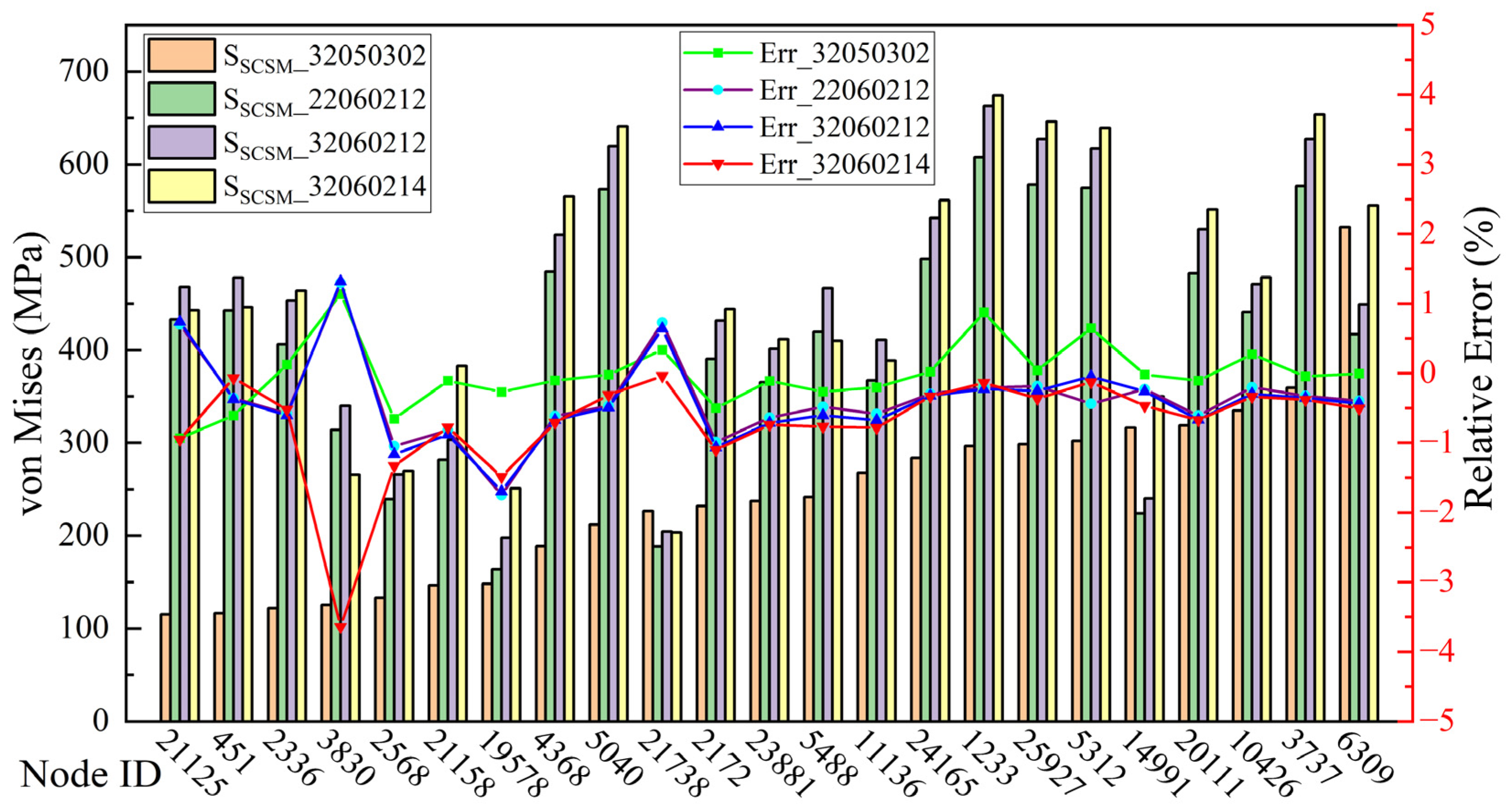
3.3. Method Validation

In order to calculate the critical location stress, the MLG geometric flexibility, shock absorber travel, real contact status, and so on should be considered to establish transient dynamics or quasi-static FEM. However, transient dynamic models are computationally intensive and difficult to converge [23,31,32], so this article adopts the quasi-static method. According to the Saint-Venant principle [33,34], for the location far away from the external forces in the whole MLG quasi-static FEM, its stress can be determined by the linear superposition relationship of the external forces. Therefore, the stress components under a certain FLC can be calculated as follows [35]:

$${\sigma }_{ij}^n=a_{ij,0}+°a_{ij,1}\cdot F_1+a_{ij,°2}\cdot F_2+a_{ij,°3}\cdot F_3+a_{ij,°4}\cdot F_4+a_{ij,°5}\cdot F_5$$

(15)

where ${\sigma }_{ij}^n$($i,j$ = 1,2,3,) represents the 6 stress components of the node n. $F_u$($u$ = 1–5) represents the components of external forces on the landing gear under a certain fatigue condition, $a_{ij,0}$~$a_{ij,5}$ are the stress influence factors of each force component $F_u$.

Substitute the Equation (7) into Equation (15), and take the external force component $F_u$ as the unit load $P_{uv}$ (see Table 4); after some deduction, the stress component superposition formula is obtained as follows [36,37]:

$${\sigma }_{ij}^n={\displaystyle {\sum }_u{\displaystyle {\sum }_v{c}_{uv}\cdot s_{ij,uv}^n}}$$

(16)

where $c_{uv}$ is the load coefficients. $s_{ij}^n$ is the stress component of node n under the unit load case, and its value can be obtained by finite element simulation under each unit load $P_{uv}$.

Meanwhile, the invariant of stress tensor and the stress equation of state is as follows:

$$\left\{\begin{array}{l}{I}_1={\sigma }_{11}+{\sigma }_{22}+{\sigma }_{33}\hfill \\ I_2={\sigma }_{11}{\sigma }_{22}+{\sigma }_{22}{\sigma }_{33}+{\sigma }_{33}{\sigma }_{11}-{\sigma }_{12}^2-{\sigma }_{23}^2-{\sigma }_{31}^2\hfill \\ I_3={\sigma }_{11}{\sigma }_{22}{\sigma }_{33}+2{\sigma }_{12}{\sigma }_{23}{\sigma }_{31}-{\sigma }_{11}{\sigma }_{23}^2-{\sigma }_{22}{\sigma }_{31}^2-{\sigma }_{33}{\sigma }_{12}^2\hfill \end{array}\right.$$

(17)

$${\sigma }^3-I_1{\sigma }^2+I_2\sigma -I_3=0$$

(18)

where ${\sigma }_{ij}$($i,j$ = 1,2,3), respectively, represent stress components, among them, ${\sigma }_{11}$, ${\sigma }_{22}$, and ${\sigma }_{33}$ are the normal stress, and ${\sigma }_{12}$, ${\sigma }_{23}$, and ${\sigma }_{13}$ are the shear stress.

By combining Equations (16)–(18), the principal stresses ${\sigma }_1$, ${\sigma }_2$, and ${\sigma }_3$ under a certain FLC can be solved. Finally, the absolute maximum principal (AMP) stress and the signed von Mises (SVM) stress under any actual FLC can be calculated as follows:

$${\sigma }_{AMP}=\left\{\begin{array}{ll}{\sigma }_1\hfill & ,\left|{\sigma }_3\right|\le \left|{\sigma }_1\right|\hfill \\ {\sigma }_3\hfill & ,\left|{\sigma }_3\right|>\left|{\sigma }_1\right|\hfill \end{array}\right.$$

(19)

$${\sigma }_{SVM}={\displaystyle \frac{{\sigma }_{AMP}}{\left|{\sigma }_{AMP}\right|}}\sqrt{{\displaystyle \frac{{\left({\sigma }_1-{\sigma }_2\right)}^2+{\left({\sigma }_2-{\sigma }_3\right)}^2+{\left({\sigma }_1-{\sigma }_3\right)}^2}{2}}}$$

(20)

According to the SAT actual fatigue condition, the assembly of FEM is adjusted, and the loads in Table 4 are applied. Then, refer to Figure 4 for FE simulation to extract the stress of the unit load cases. Using the stress component superposition method (SCSM) described in Formulas (16)–(20) and the stress influence coefficients in Figure 3, the fatigue strength (corresponding to the signed Mises stress in this article) can be calculated, denoted as $S_{SCSM}$. Then, the loads under this fatigue condition are directly applied, and the von Mises stress is obtained by direct FE simulation (DFES), denoted as $S_{DFES}$.

Subsequently, the von Mises stress of the 4 fatigue conditions is obtained by the SCSM and DFES method, respectively. Randomly select 23 nodes as the concerned area, and the comparison of stress calculated by the two methods is shown in Figure 6.

From Figure 6, it can be seen that the maximum relative error of the stress calculated by the SCSM and DFES method is −3.64%, so all the relative errors are within ±5%. This suggests that the SCSM is a feasible and appropriate method.

It is worth noting that we only compare some hot nodes under several fatigue conditions here. When conducting fatigue assessment, the interest nodes cannot be selected in regions with singular stress or lower stress. Otherwise, the calculation error of these two methods will not be guaranteed. In order to improve the universality and robustness of the SCSM, it is necessary to combine the stress component interpolation method, as detailed in Section 4.2.

4. Fatigue Life Evaluation of the Main Fitting

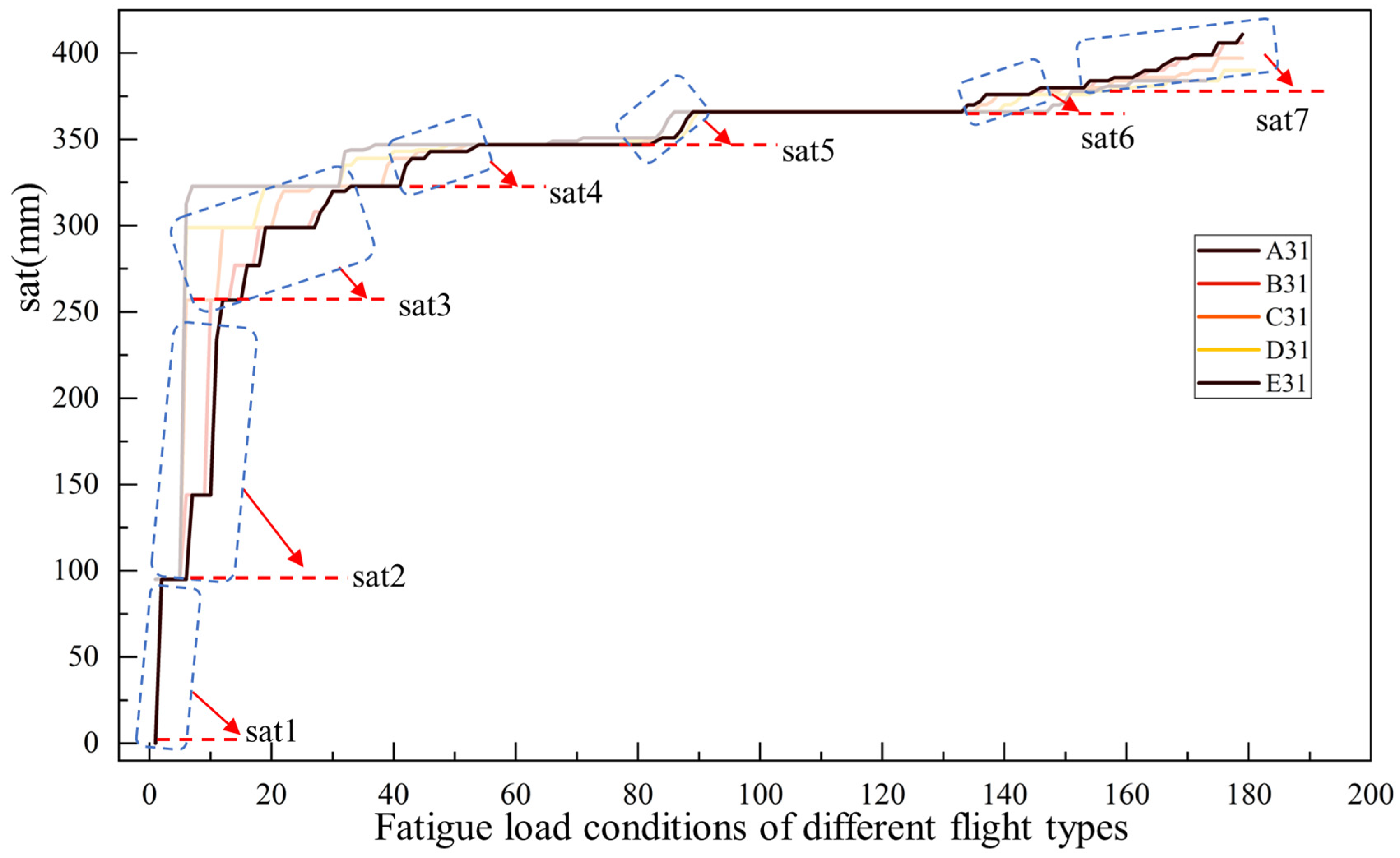
4.1. Equivalent Simplification of SAT

Each flight mission can be designated as a certain flight type. Each flight type consists of hundreds of fatigue conditions arranged in a certain sequence. Each fatigue condition with a certain SAT corresponds to a FEM. Therefore, if each fatigue condition is simulated according to its actual SAT, it will consume a lot of computational resources and time. To reduce the number of FE simulations, firstly, sort the SAT of fatigue conditions under various flight types, and then simplify them into several fixed values, as shown in Figure 7. Considering the distribution of SAT corresponding to fatigue load conditions in each flight type, the seven values selected in this paper are 0%, 20%, 50%, 70%, 75%, 80%, and 85% of the maximum stroke of the SA ($sa{t}_{max}$ = 476 mm), respectively. In order to make the fatigue life conservative, the larger SAT value should be simplified toward a smaller value.

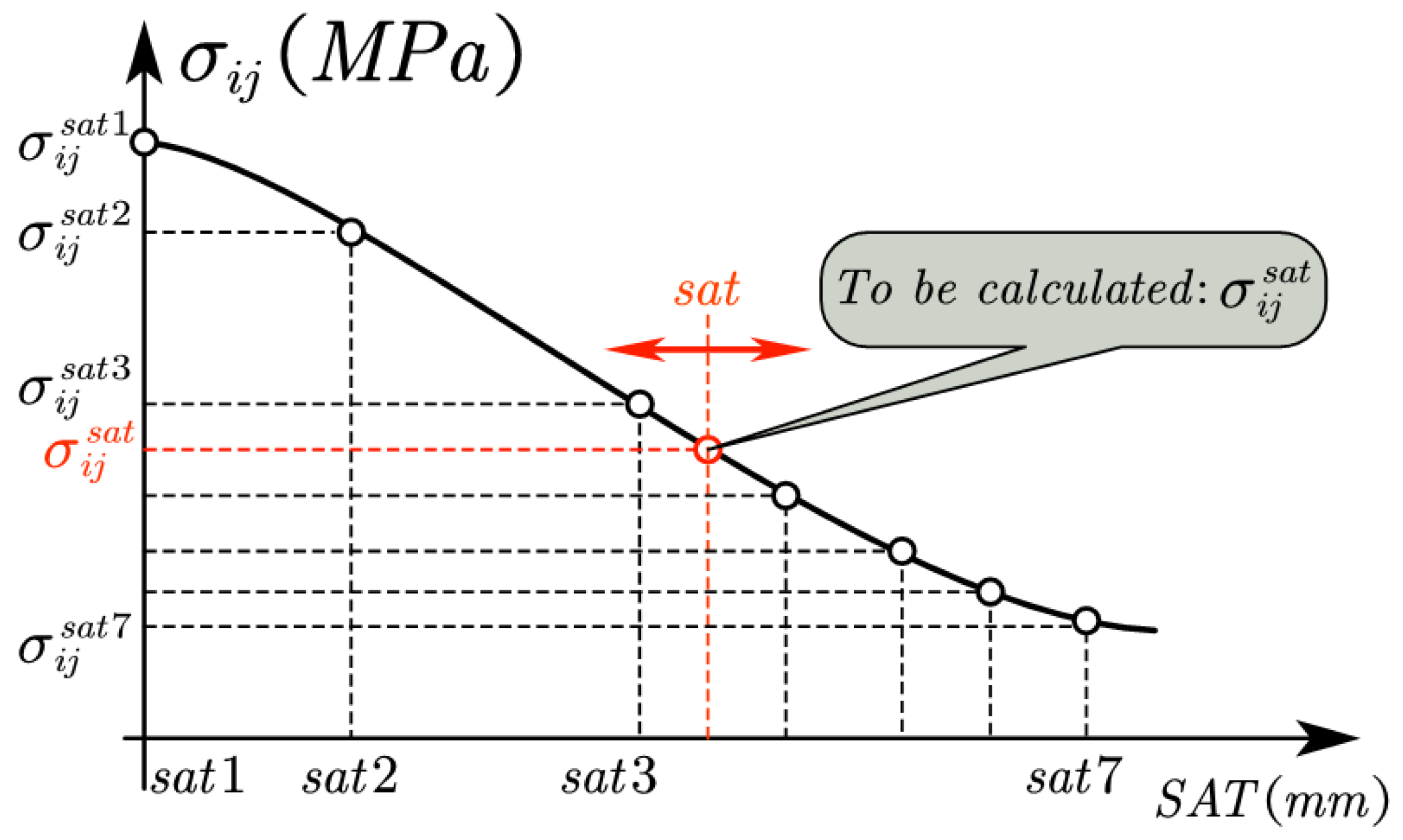
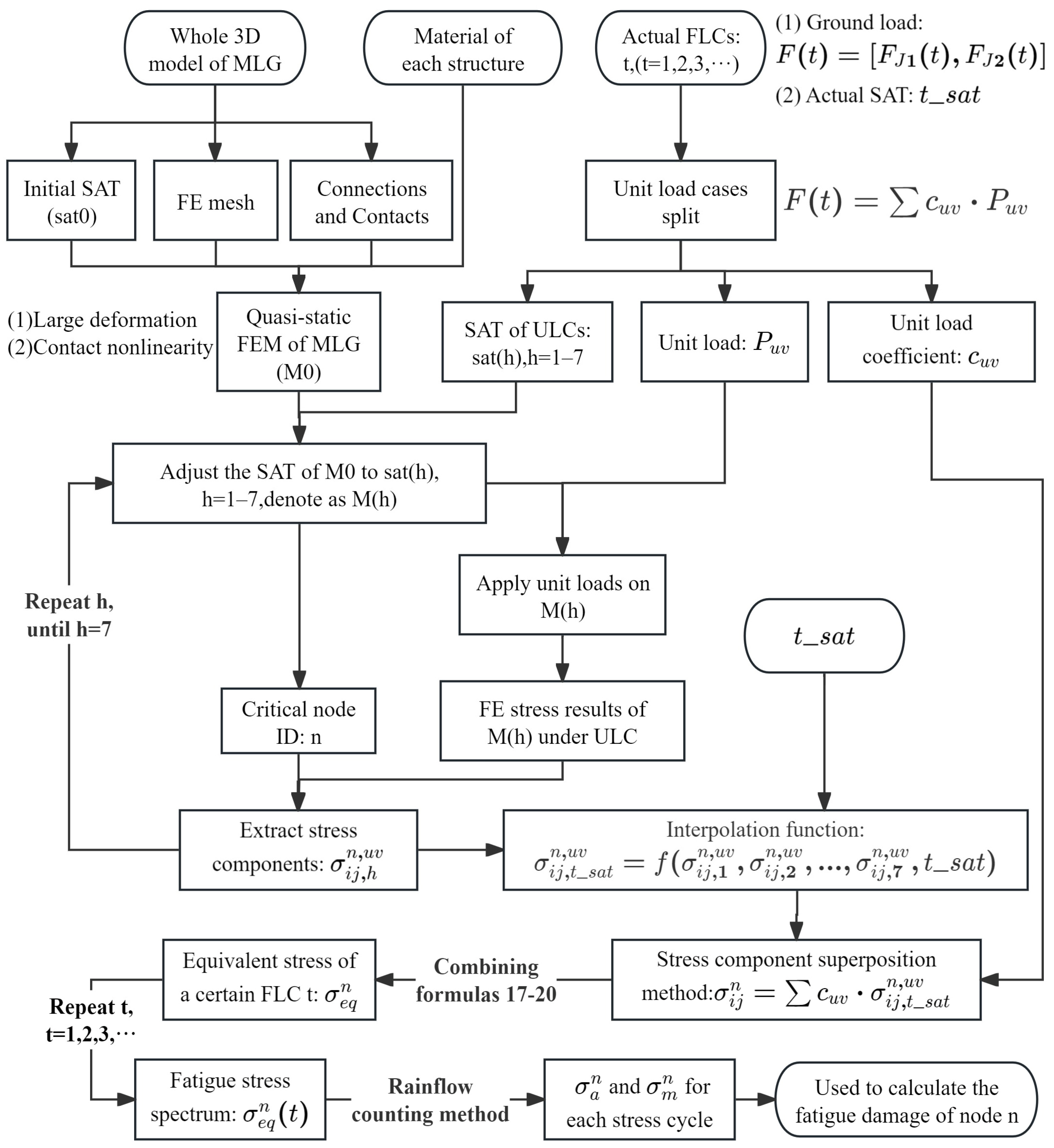
4.2. Computational Methodology for Dynamic Stress

According to Figure 7 and Table 4, this article requires applying 12 unit loads to the FEM of the MLG with seven specified SATs. This means that a total of 7 × 12 = 84 quasi-static FE simulations are needed to obtain the stress of those unit load cases. As shown in Figure 8, for any actual fatigue condition (with the stroke of the SA set as sat), its stress component under a certain unit load can be obtained by interpolating the stress components of the seven FEMs with those specified strokes of the SA.

Subsequently, according to Equations (16) to (20) and Figure 8, the fatigue stress under any actual working conditions is calculated based on the stress component superposition method, and the stress time history (i.e., stress spectrum) calculation process for any node is shown in Figure 9. That is to say, considering that the SAT of the MLG varies under different fatigue conditions, and to reduce the number of finite element (FE) simulations, this article simplifies all the SAT experienced by the MLG into seven specific values, so as to establish seven quasi-static FEMs of the MLG with those specified SATs. In this way, the fatigue stress of the MLG with any actual SAT can be obtained by interpolating the stress components of the seven FEMs.

Finally, using the load coefficients corresponding to each unit load case (see Figure 3) and the stress component superposition method (see Figure 9), the stress spectra of the four concerned nodes are calculated as shown in Figure 10.

4.3. Fatigue Life Calculation

According to the stress time history of the four concerned nodes in Figure 10 above, the rainflow counting [38,39] is performed as shown in Figure 11. Thus, the stress amplitude and mean value of each stress cycle can be obtained.

If the average stress in the real stress cycle is different from the S-N curve of the material, that is, the stress ratio R is different, then the stress amplitude must be corrected. Normally, the S-N curve of the material is measured based on the condition that the average stress is 0 (i.e., the stress ratio R = −1). References [40,41,42] give the general form of the average stress correction model as follows:

$${\left({\displaystyle \frac{{\sigma }_a}{{\sigma }_{ar}}}\right)}^a+{\left({\displaystyle \frac{{\sigma }_m}{c\cdot {\sigma }_b}}\right)}^b=1$$

(21)

where ${\sigma }_a$ and ${\sigma }_m$ represent the amplitude and mean values in stress cycles, respectively. ${\sigma }_b$ is the ultimate tensile strength limit of the material. ${\sigma }_{ar}$ is the equivalent stress after average stress correction. a, b, and c are the parameters of the mean stress correction model.

In most engineering practices, the Goodman correction model is commonly used to consider the influence of average stress in landing gear stress cycles on structural fatigue life [1,29]. Therefore, this paper takes a = 1, b = 1, c = 1 to correct the average stress to the S-N curve with a stress ratio of R = −1, and Formula (21) becomes

$${\displaystyle \frac{{\sigma }_a}{{\sigma }_{ar(R=-1)}}}+{\displaystyle \frac{{\sigma }_m}{{\sigma }_b}}=1$$

(22)

In addition, the material of the MF that needs to be evaluated for fatigue life is 300M high-strength steel. And its S-N curve was tested by smooth specimen as shown in Figure 12. It is worth noting that the S-N curves must refer to un-notched specimens ($K_t$ = 1.0), since the influence of notch on local stress is included in the full-size FEM.

To improve the fitting accuracy of the experimental data for the 300M steel in Figure 12, this paper adopts a three-parameter S-N curve equation [43,44,45] as follows:

$$\lg N=A_1+A_2\cdot \lg \left(S_{\max }-A_3\right)$$

(23)

where the fitting coefficients of the 95%/95% S-N curve are as follows: A1 = 12.7, A2 = 3.4, and A3 = 730.

For the stress cycles in Figure 11, the equivalent stress ${\sigma }_{ar}$ is calculated through equation (22). Then, the equivalent stress is substituted into Formula (23) or Figure 12 to obtain the fatigue damage corresponding to each stress cycle. Eventually, based on the Palmgren–Miner cumulative damage rule [29,40], see Formula (24), and taking the fatigue scatter factor [6] as 5.0, see Formula (25), the fatigue life of the four dangerous nodes on the MF are evaluated as shown in

Table 5. The fatigue life of four dangerous nodes on the MF.

Node ID	${\mathit{N}}_{\mathit{f}}$/Landings
5312	53,164
5488	60,272
21125	78,481
19578	83,775

below.

$$D={\displaystyle \sum \frac{n_i}{N_{fi}}}$$

(24)

where $n_i$ is the cycle number of a certain stress amplitude, $N_{fi}$ is the number of cycles that cause failure at this stress level and can be obtained through Formula (23), $D$ is the total fatigue damage.

$$N_f={\displaystyle \frac{D_C}{D}}/L_f$$

(25)

where $N_f$ is the predicted lifespan. $L_f$ = 5.0 is the fatigue scatter factor. When combined with the 95%/95% S-N curve to predict lifespan, the critical damage of the material is $D_C$ = 1.0.

5. Result Analysis and Discussion

5.1. Effect of SAT on the Load Transmission

We applied four unit load conditions at points O1 and O2 to FEMs with five different SATs, namely heading force P1_case1 = (+20,+25) kN, P1_case2 = (+25,+20) kN, and side force P3_case3 = (+100,+125) kN, P3_case4 = (+125,+100) kN. Extract the contact reaction force of position P that connects the Main Fitting and the shock absorber. Then, compare it with the theoretical calculation value as shown in Figure 13:

From Figure 13, it can be seen that the force transmitted from the unit ground loads to the Main Fitting decreases with the increase in SAT, and the maximum relative error is −8.21%, which also indicates that the FEM established in this article is reasonable. In addition, from Formula (9), the vertical load is inversely proportional to the SAT. Therefore, the vertical stiffness of the LG is also related to the SAT, which in turn affects its stress. To conclude, SAT plays an important role in the transmission of force.

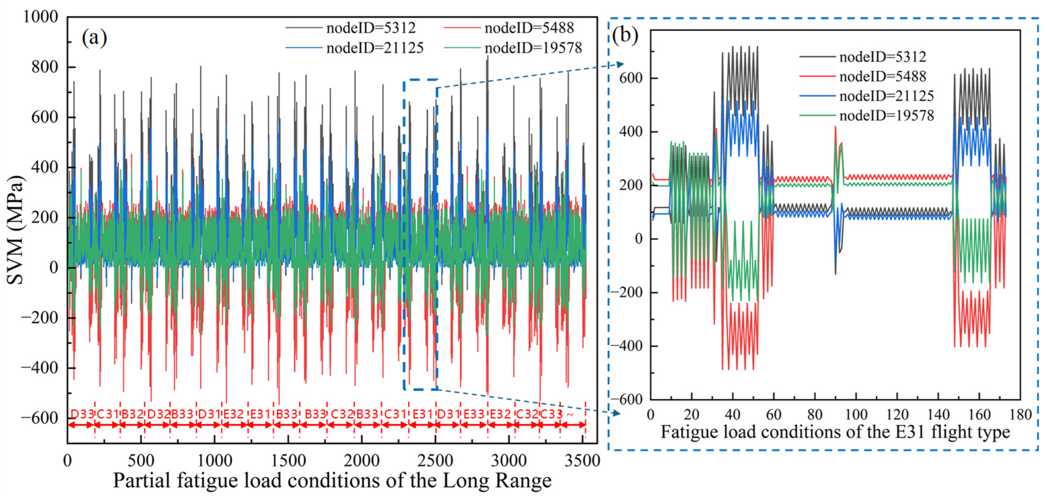
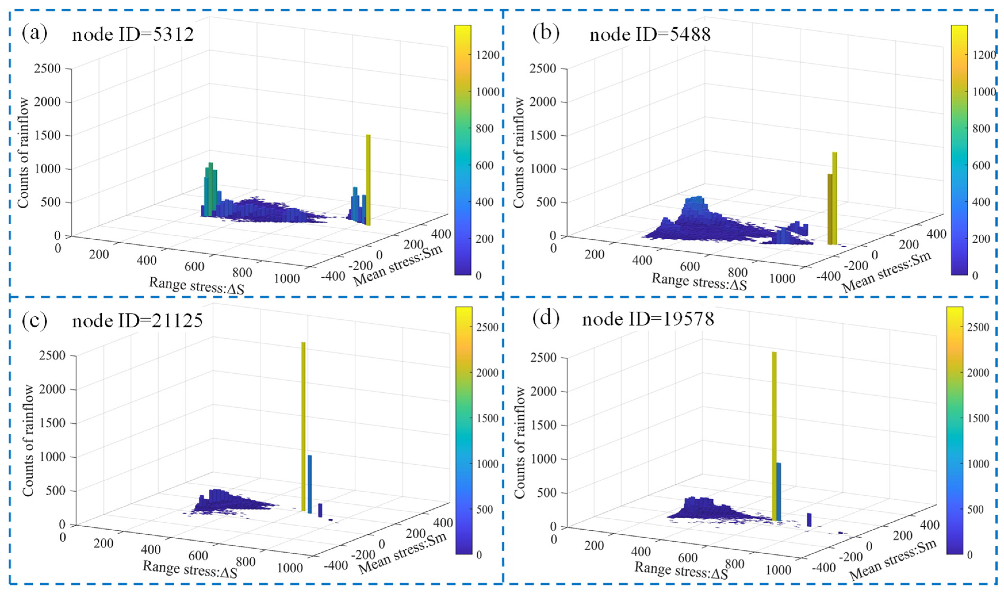
5.2. Effect of SAT on the Node Stress

In order to quantitatively analyze the influence of SAT on stress, 13 symmetrical loads are applied in five different FEMs of SAT, and their von Mises stress of node 21125 is obtained as shown in Figure 14 below.

As can be seen from Figure 14, under the same loads, the stress decreases with the increase in SAT. In addition, Figure 14a shows that the direction and uneven distribution of the heading force have a certain influence on stress. Figure 14b indicates that stress is sensitive to the uneven distribution of vertical forces. Figure 14c illustrates that the direction of side force has a certain influence on the stress. Figure 14d shows that the uneven distribution of side torque is not sensitive to the influence of stress.

In summary, in order to obtain the fatigue stress situation, it is necessary to make SAT consistent with the actual working conditions. When the fatigue load spectrum is determined, the fatigue stress of the MF is also related to the SAT.

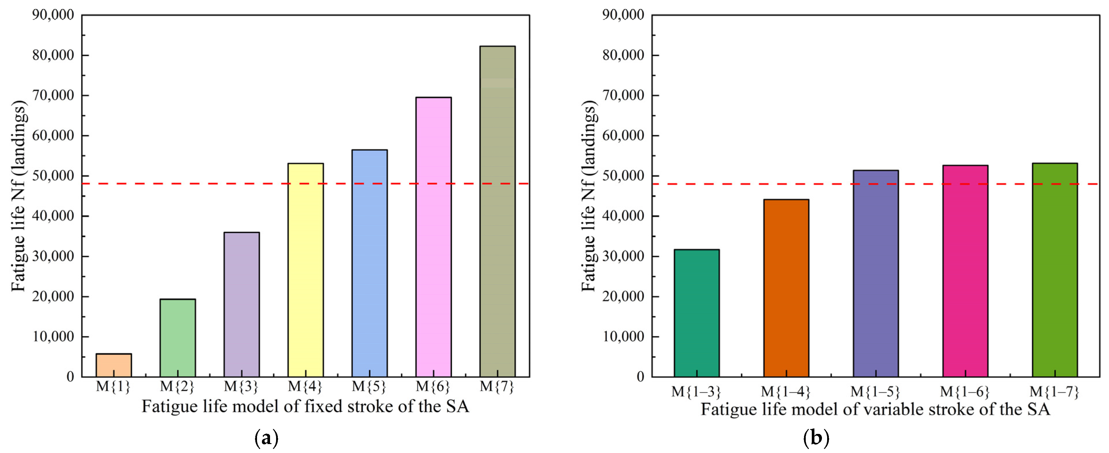
5.3. Effect of SAT on Fatigue Life Evaluation

Adjust the FE simulation model to the specified compression stroke of the SA, namely sat{h} = {0%, 20%, 50%, 70%, 75%, 80%, 85%}$·sa{t}_{max}$, h = 1–7, corresponding to fatigue life prediction models labeled as M1~M7. Specifically, for any M{h} model, apply the same unit load cases, and combine the stress results with the load scale coefficient to obtain the stress spectrum. Finally, calculating the fatigue life as shown in Figure 15a, it can be seen that the maximum difference in fatigue life of the fixed stroke prediction models is 14.3 times, indicating that the SAT has a significant impact on the fatigue life evaluation of the MLG.

Establish different fatigue life simulation models based on the interpolation calculation methods with several specific SATs proposed in Figure 9, and the lifespan results are shown in Figure 15b. It can be seen that the fatigue life of the variable stroke models based on M{1–3} and M{1–4} differs significantly compared to M{1–5}, M{1–6}, and M{1–7}, with a maximum difference of 1.68 times. But the fatigue life changes in the M{1–5}, M{1–6}, and M{1–7} models are relatively small, only 1.05 times, indicating that the life prediction model tends to be stable, and increasing the number of SATs cannot effectively improve the life prediction accuracy. Therefore, this article suggests using at least five SATs to establish an interpolated model of life prediction.

From Figure 15, we can see that SAT is a significant influencing factor in the prediction of the LG’s fatigue life. In the fatigue life prediction model considering the variable stroke of the shock absorber, blindly increasing the number of SATs does not significantly improve the accuracy of life prediction. The reason behind this is that the SAT affects the stress response of the landing gear (see Figure 6 and Figure 9), and several specific SATs can accurately approximate the stress calculated by the interpolation and superposition method proposed in this paper to the direct finite element simulation method. It should be emphasized that we must carefully select these representative SATs based on the distribution pattern of SATs for all fatigue conditions. On the other hand, although the method proposed in Figure 9 has been proven to be effective, we still recommend using the direct finite element simulation method when there are fewer fatigue conditions (≤100), which can maximize consistency with actual conditions. However, when there are many fatigue conditions, using the stress component interpolation and superposition method proposed in this article can greatly improve the efficiency of calculations and ensure a certain level of accuracy.

6. Conclusions

In this study, we introduced a stress component interpolation and superposition method for calculating the stress spectrum based on the finite element models with several specific strokes of the shock absorber under unit load cases. Compared with direct FE simulation analysis on thousands of actual working conditions, it saves a lot of computational time and resources, and the relative errors of stress are almost within ±5%. The fatigue life prediction model for the variable stroke of the MLG proposed in this article is more realistic and effective to consider dynamic stress problems under various load conditions. For the simulation of the fatigue life of the main landing gear, some conclusions are drawn as follows:

(1) Through the study of the force transmission path and spatial force system decomposition of the MLG, we summarized the magnitude and direction of loads for 14 basic unit load cases, and the forces of a certain fatigue condition can be expressed as the superposition of the force of each unit load case and its load scale coefficient. To improve the efficiency of fatigue life calculation and reduce the number of FE simulations, the shock absorber travel should be simplified to seven specified basic values, and the stress under any fatigue condition can be obtained by interpolating the stress components of these basic unit load cases.

(2) The shock absorber travel plays an important role in the transmission of force and the stress distribution of the LG. Generally speaking, when the same load is applied to the LG, the stress decreases with the increase in the stroke of the shock absorber.

(3) The shock absorber travel has a significant impact on the fatigue life of the Main Fitting of the LG. When we use a fatigue life prediction model with the fixed stroke of the shock absorber to evaluate the lifespan of the Main Fitting, the prediction lifespan may differ by 14.3 times. Under identical load conditions, the fatigue prediction model with a larger stroke of the shock absorber corresponds to a shorter calculated fatigue life.

(4) To make the fatigue life prediction of the LG more stable and accurate, the variable stroke model for fatigue life prediction should at least consider five specific strokes of the shock absorber. Based on the stress interpolation and superposition of unit load cases under different shock absorber travel, an efficient and practical approach is provided for the robust design of the structural fatigue life of the LG.

(5) The minimum prediction fatigue life of the Main Fitting of the MLG is 53,164 landings, which is greater than its target service life (48,000 landings). This indicates that the fatigue life of the Main Fitting meets its design requirements. Although the fatigue life simulation and prediction of the LG introduced in this article is of great significance for the product development and design iteration, for airworthiness certification, full-scale fatigue testing should be arranged for verification in the future.

In terms of the practical application of landing gear, the method proposed in this article can help us quickly iterate product design from the perspective of fatigue performance, design a suitable full-size fatigue test bench, verify the rationality of the load spectrum we have prepared, and quickly inform the impact of material changes on fatigue life from the perspective of the whole landing gear, etc.

References

1. Kang, B.-H.; Choi, S.-B. Design, Structure Analysis and Shock Control of Aircraft Landing Gear with MR Damper. Smart Mater. Struct. 2024, 33, 055049. [Google Scholar] [CrossRef]
2. Li, W.; Chen, S.; Chu, Y.; Huang, P.; Yan, G. Wide-Range Fiber Bragg Grating Strain Sensor for Load Testing of Aircraft Landing Gears. Optik 2022, 262, 169290. [Google Scholar] [CrossRef]
3. Wang, Y.; Zhang, X.; Dong, X.; Yao, W. Multiaxial Fatigue Assessment for Outer Cylinder of Landing Gear by Critical Plane Method. Proc. Inst. Mech. Eng. G J. Aerosp. Eng. 2022, 236, 993–1005. [Google Scholar] [CrossRef]
4. Raouf, I.; Kumar, P.; Cheon, Y.; Tanveer, M.; Jo, S.-H.; Kim, H.S. Advances in Prognostics and Health Management for Aircraft Landing-Progress, Challenges, and Future Possibilities. Int. J. Precis. Eng. Manuf. Green Technol. 2024, 12, 301–320. [Google Scholar] [CrossRef]
5. Yan, S.; Xue, P.; Liu, L.; Zahran, M.S. Optimization of Landing Gear under Consideration of Vibration Comfort for Civil Aircraft. Aircr. Eng. Aerosp. Technol. 2024, 96, 378–386. [Google Scholar] [CrossRef]
6. Fu, Y.; Fu, H.; Zhang, S. A Novel Safe Life Extension Method for Aircraft Main Landing Gear Based on Statistical Inference of Test Life Data and Outfield Life Data. Symmetry 2023, 15, 880. [Google Scholar] [CrossRef]
7. Chiariello, A.; Carandente Tartaglia, C.; Arena, M.; Quaranta, V.; Bruno, G.; Belardo, M.; Castaldo, M. Vibration Qualification Campaign on Main Landing Gear System for High-Speed Compound Helicopter. Aerospace 2024, 11, 130. [Google Scholar] [CrossRef]
8. Jiang, Y.; Feng, G.; Tang, H.; Zhang, J.; Jiang, B. Effect of Coulomb Friction on Shimmy of Nose Landing Gear under Time-Varying Load. Tribol. Int. 2023, 188, 108828. [Google Scholar] [CrossRef]
9. Wang, X.H.; Luo, H.W. Research and Application Progress in Ultra-High Strength Stainless Steel for Aircraft Landing Gear. Cailiao Gongcheng/J. Mater. Eng. 2019, 47, 9. [Google Scholar] [CrossRef]
10. Liu, P.; Zhang, J.; Tang, H.; Duan, H.; Jiang, B. Residual Fatigue Life Prediction Based on a Novel Improved-Halford Model Considering Loading Interaction Effect. Heliyon 2024, 10, e36716. [Google Scholar] [CrossRef]
11. Skorupka, Z. Dynamic Fatigue Tests of Landing Gears. Fatigue Aircr. Struct. 2020, 2020, 69–77. [Google Scholar] [CrossRef]
12. Bag, A.; Delbergue, D.; Ajaja, J.; Bocher, P.; Lévesque, M.; Brochu, M. Effect of Different Shot Peening Conditions on the Fatigue Life of 300 M Steel Submitted to High Stress Amplitudes. Int. J. Fatigue 2020, 130, 105274. [Google Scholar] [CrossRef]
13. Wu, B.; Shi, Y.; Yin, Y. Optimization Design of Landing Gear Structure Based on Fatigue Life Constraint. In Proceedings of the Journal of Physics: Conference Series; IOP Publishing: Bristol, UK, 2022; Volume 2403. [Google Scholar]
14. Schmidt, R.K. The Design of Aircraft Landing Gear; SAE International: Warrendale, PA, USA, 2021. [Google Scholar]
15. El Mir, H.; Perinpanayagam, S. Certification of Machine Learning Algorithms for Safe-Life Assessment of Landing Gear. Front. Astron. Space Sci. 2022, 9, 896877. [Google Scholar] [CrossRef]
16. EASA. Certification Specifications and Acceptable Means of Compliance for Large Aeroplanes CS-25. 2018. Available online: https://www.easa.europa.eu/en/document-library/certification-specifications/cs-25-amendment-14 (accessed on 12 December 2024).
17. Giannella, V.; Baglivo, G.; Giordano, R.; Sepe, R.; Citarella, R. Structural FEM Analyses of a Landing Gear Testing Machine. Metals 2022, 12, 937. [Google Scholar] [CrossRef]
18. Dziendzikowski, M.; Kurnyta, A.; Reymer, P.; Kurdelski, M.; Klysz, S.; Leski, A.; Dragan, K. Application of Operational Load Monitoring System for Fatigue Estimation of Main Landing Gear Attachment Frame of an Aircraft. Materials 2021, 14, 6564. [Google Scholar] [CrossRef]
19. Fang, F.; Qiu, L.; Yuan, S.; Ren, Y. Dynamic Probability Modeling-Based Aircraft Structural Health Monitoring Framework under Time-Varying Conditions: Validation in an in-Flight Test Simulated on Ground. Aerosp. Sci. Technol. 2019, 95, 105467. [Google Scholar] [CrossRef]
20. Qiu, L.; Yuan, S.; Boller, C. An Adaptive Guided Wave-Gaussian Mixture Model for Damage Monitoring under Time-Varying Conditions: Validation in a Full-Scale Aircraft Fatigue Test. Struct. Health Monit. 2017, 16, 501–517. [Google Scholar] [CrossRef]
21. Dai, X.; Liu, L.; Xu, Q.; Xu, F.; Hu, X. Research on the Control Technology of Aircraft Landing Gear Buffer Variable Stroke. J. Phys. Conf. Ser. 2024, 2820, 12010. [Google Scholar] [CrossRef]
22. Chen, C.; Hu, B.; Chen, X.; Chai, Y.; Zhang, C. Variable Stroke Fatigue Test for Aircraft Landing Gears. Proc. Inst. Mech. Eng. Part C J. Mech. Eng. Sci. 2024. [Google Scholar] [CrossRef]
23. Zhu, Z.H.; Larosa, M.; Ma, J. Fatigue Life Estimation of Helicopter Landing Probe Based on Dynamic Simulation. J. Aircr. 2009, 46, 1533–1543. [Google Scholar] [CrossRef]
24. Infante, V.; Fernandes, L.; Freitas, M.; Baptista, R. Failure Analysis of a Nose Landing Gear Fork. Eng. Fail. Anal. 2017, 82, 554–565. [Google Scholar] [CrossRef]
25. Freitas, M.; Infante, V.; Baptista, R. Failure Analysis of the Nose Landing Gear Axle of an Aircraft. Eng. Fail. Anal. 2019, 101, 113–120. [Google Scholar] [CrossRef]
26. Raković, D.; Simonović, A.; Grbović, A.; Radović, L.; Vorkapić, M.; Krstić, B. Fatigue Fracture Analysis of Helicopter Landing Gear Cross Tube. Eng. Fail. Anal. 2021, 129, 105672. [Google Scholar] [CrossRef]
27. Raičević, N.; Grbović, A.; Kastratović, G.; Vidanović, N.; Sedmak, A. Fatigue Life Prediction of Topologically Optimized Torque Link Adjusted for Additive Manufacturing. Int. J. Fatigue 2023, 176, 107907. [Google Scholar] [CrossRef]
28. Xie, H.; Yang, G.; Sun, J.; Sai, W.; Zeng, W. Anti-Fatigue Optimization of the Twisting Force Arm of Landing Gear Based on Kriging Approximate Sequential Optimization Method. J. Chin. Inst. Eng. Trans. Chin. Inst. Eng. Ser. A 2024, 47, 2274086. [Google Scholar] [CrossRef]
29. Xue, C.J.; Dai, J.H.; Wei, T.; Liu, B.; Deng, Y.Q.; Ma, J. Structural Optimization of a Nose Landing Gear Considering Its Fatigue Life. J. Aircr. 2012, 49, 225–236. [Google Scholar] [CrossRef]
30. Shao, H.; Li, D.; Kan, Z.; Zhao, S.; Xiang, J.; Wang, C. Analysis of Catapult-Assisted Takeoff of Carrier-Based Aircraft Based on Finite Element Method and Multibody Dynamics Coupling Method. Aerospace 2023, 10, 1005. [Google Scholar] [CrossRef]
31. Candon, M.; Esposito, M.; Fayek, H.; Levinski, O.; Koschel, S.; Joseph, N.; Carrese, R.; Marzocca, P. Advanced Multi-Input System Identification for next Generation Aircraft Loads Monitoring Using Linear Regression, Neural Networks and Deep Learning. Mech. Syst. Signal Process. 2022, 171, 108809. [Google Scholar] [CrossRef]
32. Suresh, P.S.; Sura, N.K.; Shankar, K.; Radhakrishnan, G. Synthesis of Landing Dynamics on Land-Base High Performance Aircraft Considering Multi-Variate Landing Conditions. Mech. Based Des. Struct. Mach. 2023, 51, 1946406. [Google Scholar] [CrossRef]
33. Di Lorenzo, D.; Rodriguez, S.; Champaney, V.; Germoso, C.; Beringhier, M.; Chinesta, F. Damage Identification Technique by Model Enrichment for Structural Problems. Results Eng. 2024, 23, 102389. [Google Scholar] [CrossRef]
34. Marin, M.; Öchsner, A.; Craciun, E.M. A Generalization of the Saint-Venant’s Principle for an Elastic Body with Dipolar Structure. Contin. Mech. Thermodyn. 2020, 32, 269–278. [Google Scholar] [CrossRef]
35. Dong, G.; Zhang, M.; Wei, L.; Zhang, Y. Study on High Cycle Fatigue Criteria under Multi-Axial Random Loads of Chassis Parts. Zhongguo Jixie Gongcheng/China Mech. Eng. 2021, 32, 2294. [Google Scholar] [CrossRef]
36. Zhang, S.; Le, C.; Gain, A.L.; Norato, J.A. Fatigue-Based Topology Optimization with Non-Proportional Loads. Comput. Methods Appl. Mech. Eng. 2019, 345, 805–825. [Google Scholar] [CrossRef]
37. Mi, C.; Gu, Z.; Yang, Q.; Nie, D. Frame Fatigue Life Assessment of a Mining Dump Truck Based on Finite Element Method and Multibody Dynamic Analysis. Eng. Fail. Anal. 2012, 23, 18–26. [Google Scholar] [CrossRef]
38. Liu, K.G.; Yan, C.L.; Zhang, S.M. Estimation of Fatigue Damage of Airplane Landing Gear. Front. Mech. Eng. China 2006, 1, 424–428. [Google Scholar] [CrossRef]
39. ASTM E1049-85; Standard Practices for Cycle Counting in Fatigue Analysis. ASTM International: West Conshohocken, PA, USA, 2011.
40. Zhang, Q.L.; Hu, L.; Gao, X.F. Fatigue Life Prediction of Steel Spiral Cases in Pumped-Storage Power Plants: Factors to Be Considered. Eng. Fail. Anal. 2024, 157, 107908. [Google Scholar] [CrossRef]
41. Lian, Y.; Zhao, R.; Yu, K.; Zhu, Y. P-S-N Surfaces of Lifting Lug Structure Based on Extremely Small Samples. Eng. Fail. Anal. 2024, 162, 108457. [Google Scholar] [CrossRef]
42. Liu, Y.; Paggi, M.; Gong, B.; Deng, C. A Unified Mean Stress Correction Model for Fatigue Thresholds Prediction of Metals. Eng. Fract. Mech. 2020, 223, 106787. [Google Scholar] [CrossRef]
43. Hoole, J.; Sartor, P.; Booker, J.; Cooper, J.; Gogouvitis, X.V.; Schmidt, R.K. Systematic Statistical Characterisation of Stress-Life Datasets Using 3-Parameter Distributions. Int. J. Fatigue 2019, 129, 105216. [Google Scholar] [CrossRef]
44. Tan, X.; Li, Q.; Wang, G.; Xie, K. Three-Parameter P-S-N Curve Fitting Based on Improved Maximum Likelihood Estimation Method. Processes 2023, 11, 634. [Google Scholar] [CrossRef]
45. Rice, R.; Jackson, J.; Bakuckas, J.; Thompson, S. Metallic Materials Properties Development and Standardization (MMPDS); 2003. Available online: https://ntrl.ntis.gov/NTRL/dashboard/searchResults/titleDetail/PB2003106632.xhtml (accessed on 12 December 2024).
Figure 1. Loads transmission of MLG: (a) side view of aircraft; (b) schematic diagram of different coordinate systems; (c) 3D physical model of the left MLG; (d) components of oleo-pneumatic shock absorber.
Aerospace 12 00042 g001
Figure 2. Schematic diagram of torque decomposition: (a) front view of the Wheel axle for equivalent of M D O ; (b) vertical view for equivalent of M v O ; (c) detailed view of Brake Assy; (d) side view for equivalent of M S O ; (e) section view of brake device.
Aerospace 12 00042 g002
Figure 3. Load coefficients of ULC for E31 flight type under LR.
Aerospace 12 00042 g003
Figure 4. Quasi-static finite element model: (a) boundary conditions; (b,c) internal connection situation of the SA; (d) Pressure on the inner surface of the MF; (e) loading diagram; (f) simulation stress cloud diagram.
Aerospace 12 00042 g004
Figure 5. Contact reaction force of P and Q of shock absorber where E r r _ F P = ( c a l _ F P - s i m _ F P )/ c a l _ F P , E r r _ F Q = ( c a l _ F Q - s i m _ F Q )/ c a l _ F Q .
Aerospace 12 00042 g005
Figure 6. Comparison between stress component superposition and direct FE simulation method where E r r = ( S S C S M - S D F E S )/ S S C S M is the relative error between S S C S M and S D F E S .
Aerospace 12 00042 g006
Figure 7. Diagrams of different flight types simplified to 7 SATs where A31, B31, C31, D31, and E31 represent some flight types in the Long Range. The horizontal axis represents the sequence of the FLCs sorted by SAT under different flight types.
Aerospace 12 00042 g007
Figure 8. Schematic diagram of stress component interpolation where σ i j s a t = interp1(X, Y, sat,‘spline’). Among them, interp1(-) represents the interpolation function of Matlab r2021b, and the vector X = [sat1, sat2, ~, sat7], the vector Y = [ σ i j s a t 1 , σ i j s a t 2 , ~, σ i j s a t 7 ].
Aerospace 12 00042 g008
Figure 9. Calculation process of node stress spectrum.
Aerospace 12 00042 g009
Figure 10. Stress spectra of some nodes: (a) Long Range; (b) E31 flight type.
Aerospace 12 00042 g010
Figure 11. Rainflow counting results of the stress spectrum of some dangerous nodes: (a) node 5312; (b) node 5488; (c) node 21125; (d) node 19578.
Aerospace 12 00042 g011
Figure 12. Test S-N curve of 300M steel smooth bar specimen: Kt = 1, R = −1, f = 110 Hz: (a) testing equipment; (b) sample installation status; (c) partial samples after testing; (d) test data where p and γ are the survival rate and confidence level of the S-N curve, respectively.
Aerospace 12 00042 g012
Figure 13. Comparison of the contact force of position P between FE simulation and theoretical deduction: (a) heading force conditions; (b) side force conditions.
Aerospace 12 00042 g013
Figure 14. Stress variation in node 21125 with sat: (a) stress under the action of heading force; (b) stress under the action of vertical force; (c) stress under the action of side force; (d) stress under the action of side torque.
Aerospace 12 00042 g014
Figure 15. Fatigue life values: (a) fixed stroke model; (b) variable stroke model where M{1}–M{7}, respectively, represent models simplified to a specific SAT. M{1–3} is the interpolation model that simplified to three SATs, M{1–4} is simplified to four SATs, M{1–5} is simplified to five SATs, M{1–6} is simplified to six SATs, and M{1–7} is simplified to seven SATs. The red dashed line represents the target service life (48,000 landings).
Aerospace 12 00042 g015