Neural Network and Hybrid Methods in Aircraft Modeling, Identification, and Control Problems

Abstract

Motion control of modern and advanced aircraft has to be provided under conditions of incomplete and inaccurate knowledge of their parameters and characteristics, possible flight modes, and environmental influences. In addition, various abnormal situations may occur during flight, in particular, equipment failures and structural damage. These circumstances cause the problem of a rapid adjustment of the used control laws so that the control system can adapt to the mentioned changes. However, most adaptive control schemes have a model of the control object, which plays a crucial role in adjusting the control law. That is, it is required to solve also the identification problem for dynamical systems. We propose an approach to solving the above-mentioned problems based on artificial neural networks (ANNs) and hybrid technologies. In the class of traditional neural network technologies, we use recurrent neural networks of the NARX type, which allow us to obtain black-box models for controlled dynamical systems. It is shown that in a number of cases, in particular, for control objects with complicated dynamic properties, this approach turns out to be inefficient. One of the possible alternatives to this approach, investigated in the paper, consists of the transition to hybrid neural network models of the gray box type. These are semi-empirical models that combine in the resulting network structure both empirical data on the behavior of an object and theoretical knowledge about its nature. They allow solving with high accuracy the problems inaccessible by the level of complexity for ANN models of the black-box type. However, the process of forming such models requires a very large consumption of computational resources. For this reason, the paper considers another variant of the hybrid ANN model. In it, the hybrid model consists not of the combination of empirical and theoretical elements, resulting in a recurrent network of a special kind, but of the combination of elements of feedforward networks and recurrent networks. Such a variant opens up the possibility of involving deep learning technology in the construction of motion models for controlled systems. As a result of this study, data were obtained that allow us to evaluate the effectiveness of two variants of hybrid neural networks, which can be used to solve problems of modeling, identification, and control of aircraft. The capabilities and limitations of these variants are demonstrated on several examples. Namely, on the example of the problem of aircraft longitudinal angular motion, the possibilities of modeling the motion using the NARX network as applied to a supersonic transport aircraft (SST) are first considered. It is shown that under complicated operating conditions this network does not always provide acceptable modeling accuracy. Further, the same problem, but applied to a maneuverable aircraft, as a more complex object of modeling and identification, is solved using both a NARX network (black box) and a semi-empirical model (gray box). The significant advantage of the gray box model over the black box one is shown. The capabilities of the hybrid model realizing deep learning technologies are demonstrated by forming a model of the control object (SST) and neurocontroller on the example of the MRAC adaptive control scheme. The efficiency of the obtained solution is illustrated by comparing the response of the control object with a failure situation (a decrease in the efficiency of longitudinal control by 50%) with and without adaptation.

1. Introduction

Machine learning (ML) is currently one of the most actively developing research areas. Significant advances have been made in techniques based on artificial neural networks (ANN) and reinforcement learning (RL). Among the applied problems in which ML methods are increasingly being applied, problems related to dynamical systems have received much attention. In particular, in the last two decades, efforts have been made to use artificial neural network technology both for modeling and identification of dynamical systems [1,2,3,4] and for their control [5,6,7,8]. The methods of reinforcement learning [9,10,11], especially such a variant of this approach as Approximate Dynamic Programming (ADP) [12,13,14,15], are also actively investigated for the same purposes. Various variants of the ADP approach represent a very useful tool for synthesizing feedback control laws [16], including those satisfying the requirements of optimality and adaptivity [17,18].

One of the areas in which the application of machine learning technologies is being actively explored is aircraft of various kinds and purposes. This state of affairs is caused by the complexity and variety of tasks that are assigned to aircraft. The complicating factor in this case is incomplete and inaccurate knowledge of the properties of the object under study and the conditions in which it operates. This is a typical situation for objects of this kind, which prompts the expansion of the tools that provide the solution of the required tasks. In addition, the objects of this class are characterized by the multi-mode of their use, as well as the multi-criteria character of the evaluation of the tasks solved by them.

For aircraft, as one of the most important kinds of dynamical systems, their behavior control has to be ensured under conditions of significant and diverse uncertainties in the values of their parameters and characteristics, flight modes, and environmental influences [19,20,21,22]. In addition, various abnormal situations may occur during flight, in particular equipment failures and structural damage, which must be counteracted by reconfiguring the aircraft control system [23,24,25,26]. Thus, it is necessary to operate under conditions of incomplete and inaccurate knowledge of the properties of both the aircraft and the environment in which it operates. In addition, the situation in which the aircraft finds itself at any given time may change in a significant and unpredictable way due to the occurrence of abnormal situations. The aircraft control system must be able to operate efficiently under these conditions by promptly changing the parameters and/or structure of the control laws used. Adaptive control methods allow satisfying this requirement [22,27,28,29,30].

However, the online adjustment of the control law represents only one of the functions of an adaptive control system, although it is the most important one. The reason is that most adaptive control schemes include a model of the control object, which plays a crucial role in adjusting the control law. Obtaining such a model from data on the behavior of the control object constitutes the content of the classical dynamical system identification problem [31,32]. The well-known manual on system identification [31] says, “Inferring models from observations and studying their properties is really what science is about”. To a large part this is true, but still we should not forget that models are created for certain purposes, namely, to be able to analyze the behavior of modeled systems, and in the case of controlled systems we are interested in, also to provide the synthesis of control laws for them. It is needs of this kind that largely determine the progress in the field of modeling systems.

As noted above, the properties of a control object may be inaccurately known when forming its model, or they may change for some reason already in the process of its functioning. In such a case, in adaptive systems using the object model, it is necessary to be able to promptly restore the adequacy of the model to the control object. In other words, in such systems, not only the control law but also the object model should have the property of adaptability.

Obtaining a model of an object for its use as part of an adaptive control system is closely related to three classes of problems arising in the development of aircraft of various kinds. These classes include analysis of aircraft behavior as dynamical systems [33,34,35], synthesis of control algorithms for them [36,37,38], and identification of their unknown or imprecisely known characteristics [39,40,41]. Mathematical and computer models of controlled dynamical systems play a critical role in solving problems in all three classes. In most cases, when solving these problems, the aircraft is considered a solid body with six degrees of freedom. The traditional class of mathematical models in this situation are systems of ordinary differential equations. These models, with appropriate numerical methods [42,43,44,45], are widely used in solving problems of synthesis and analysis of controlled motion of aircraft of various classes.

The methods of formation and use of the above-mentioned models of traditional type have been developed in detail and successfully used for solving a wide range of problems. However, for modern and advanced complex technical systems, including aircraft of different classes, some problems arise, the solution of which cannot be provided by traditional techniques. These problems are caused, among other things, by the needs of adaptive control systems, i.e., the need to promptly adjust the control law and the model of the control object to maintain their adequacy to the changing situation.

Additionally, the problem of creating an adaptive control system for aircraft behavior is complicated by the fact that it becomes truly effective when working with a nonlinear model of the dynamical system under consideration. As experience shows [2,32], one of the most efficient approaches to solving the modeling problem regarding nonlinear systems is the use of methods and tools of artificial neural networks (ANN). Neural network modeling allows for the building of sufficiently accurate and computationally efficient ANN models. This approach can be considered as some alternative to methods of modeling dynamical systems based on the use of differential equations. It provides, among other things, the possibility of obtaining adaptive models. At the same time, traditional neural network models of controlled dynamical systems, in particular models of NARX and NARMAX classes [2,32,46], which are recurrent neural networks, are the most commonly used for modeling controlled dynamical systems. These models are purely empirical; that is, they are black-box type models. Such models are based solely on experimental data about the behavior of the object. However, in problems of the complexity level typical for aerospace engineering, it is often impossible to achieve the required level of accuracy for this kind of empirical model, which would provide the solution to aircraft motion control problems. In addition, due to the structural organization of such models, they do not allow solving the problem of identification of characteristics of dynamical systems (e.g., aerodynamic characteristics of aircraft), which is a serious disadvantage of this class of models.

One of the most important reasons for the low efficiency of ANN models of the traditional type in tasks related to complicated technical systems is the fact that it is required to form a black-box type model, which should cover all the details of the behavior of the system under consideration. For this purpose, it is necessary to build an ANN model of high enough dimensionality, i.e., with numerous adjustable parameters in it. At the same time, it is known from the experience of ANN modeling that the higher the dimensionality of the ANN model, the larger the amount of training data required for its adjustment [46]. As a result, with the amount of experimental data that can actually be obtained for complex technical systems, it is not possible to train such models at a given level of accuracy. This, in turn, does not allow us to obtain efficient adaptive control systems.

Obviously, as the complexity of the modeling problem to be solved grows, an ANN model of greater dimensionality will be required. For this reason, it is necessary to increase the number of adjustable parameters in it to ensure the complexity of the model is adequate for this problem. As an index of the complexity of an ANN model, we will take the number of connections in it, i.e., the number of adjustable parameters of the model. This index will be further referred to as the model dimensionality. Similarly, the number of examples in the training set will be called the dimensionality of the training set. The complexity of the model depends on the following factors: (1) the number of state and control variables in the model, i.e., the sum of the dimensionality of the state space and control space of the dynamical system under consideration; (2) the ranges of change for the state and control variables; and (3) the number of value samples for each of the state and control variables. But, as noted above, the increase in the dimensionality of the ANN model causes an increase in the required amount of training data. Because of this, there is a complexity threshold for the recurrent ANN model of empirical type above which it is not possible to train the network to a level acceptable in terms of modeling accuracy.

It is well known that Richard Bellman introduced the notion of the curse of dimensionality [47,48], which characterizes the catastrophic complexity growth of solving dynamic programming problems with increasing dimensionality of the problem to be solved. A very similar phenomenon, also a kind of curse of dimensionality, takes place in modeling controlled dynamical systems using recurrent neural networks of the empirical type.

To overcome the above-mentioned difficulties, which are typical for traditional models, both in terms of differential equations and ANN models, it is suggested to use a combined approach. Its basis is ANN modeling because only in this variant is it possible to obtain adaptive models. Theoretical knowledge about the modeling object, existing in the form of ordinary differential equations (for example, traditional models of aircraft motion), is introduced in a special way into the ANN model of hybrid type (semi-empirical ANN model, gray box model). In this case, a part of the ANN model is formed on the basis of the available theoretical knowledge and does not require further adjustment (training). Only those elements that contain uncertainties, for example, the aerodynamic characteristics of the aircraft, are subject to adjustment and/or structural correction in the process of training the ANN model.

This approach results in semi-empirical ANN models that allow us to solve problems that are inaccessible to traditional ANN methods [49,50,51,52,53,54,55]. The semi-empirical approach allows us to radically reduce the dimensionality of the ANN model, which allows us to achieve the required accuracy from it using training sets that are insufficient in size for traditional ANN models. In addition, it makes it possible to identify the characteristics of the dynamical system described by nonlinear functions of many variables, e.g., coefficients of aerodynamic forces and moments.

The semi-empirical approach to ANN modeling of aircraft allows us to effectively overcome the above-mentioned model complexity threshold. As our experience shows [56,57,58,59,60,61], it can be used to successfully solve problems that are many times more complex than what is possible with empirical ANN models. The area of effective use of such models is the identification of aircraft characteristics from the available experimental data describing its behavior. However, these results are achieved at a very high cost. Namely, the computational time consumption of semi-empirical models is such that it completely excludes the possibility of their online adjustment, i.e., adaptation. Of course, without such a possibility, these models cannot be used as part of adaptive control systems. It is necessary to create some algorithms for estimating adjustments, which must be used together with a model that is not adaptive. This is a severe limitation for semi-empirical ANN models.

Another point to be noted is that recurrent neural networks (RNNs) exist in both the empirical and semi-empirical variants. Due to its dynamic nature, RNN is a very challenging object to train [46,62,63,64,65,66]. Therefore, we should look for variants of neural network-based adaptive control schemes in which we can use only feedforward networks, which are much easier to train than recurrent networks.

So, the hybrid (semi-empirical) model allows us to solve the problem of model accuracy based on the available training data. However, this model is too complex and time-consuming to train due to the dynamic (recurrent) nature of the used network. One of the options to reduce the impact of these limitations is also to build a hybrid ANN model, but this hybridization is of a quite unfamiliar nature compared with semi-empirical models. Namely, semi-empirical models combine elements based on both theoretical and empirical data on the behavior of the object under consideration. An alternative variant of the hybrid ANN model, which will be discussed below, is based on the combination of feedforward and recurrent layers as modules. In such a variant, it is possible to involve the currently well-developed methods and tools of deep neural networks and deep learning in solving the problem [67,68,69,70]. Here, the possibility of implementing algorithms for online adjustment of models appears, i.e., they are potentially suitable for their use as part of adaptive control systems.

The above-mentioned approaches to adaptive control are based on working directly with a nonlinear model of the control object. This causes considerable difficulties, which, as noted above, are due to the dynamic nature of recurrent networks. In the case of hybrid models of the second kind, the problem is somewhat mitigated since only part of the ANN model will be recurrent, but the difficulties remain, but they will not be so severe.

In our opinion, there is currently no reasonable alternative to machine learning methods and tools for creating adaptive systems for complex systems, in particular aircraft. However, as just mentioned, it is very difficult to realize object models (as well as control laws) as dynamic networks, and we would like to have more efficient methods at our disposal. In this connection, we need to search for such variants to work with a nonlinear control object, which would allow us to limit ourselves to using only feedforward networks. The training of such networks is many times easier than the learning of recurrent networks.

This requirement is satisfied by two approaches that are potentially suitable for developing adaptive systems.

The first of them is based on the linearization of the control object. This approach is traditionally used to analyze the perturbed motion of an aircraft and synthesize control laws for it. In this case, linearized models obtained by Taylor series expansion of the right-hand sides of the original nonlinear differential equations are used [33,34,35,36]. This approach severely reduces the capabilities of the resulting adaptive systems.

An alternative variant is based on online linearization of the control object. In this option, the most promising is the use of nonlinear transformation in feedback (feedback linearization), which is selected in such a way that the dynamical system closed by such feedback becomes linear [71,72,73]. At the same time, the traditional linearization used in flight dynamics problems [33,34,35] yields a model that has the required accuracy only in the single operational mode of the nonlinear system, as well as in a small neighborhood of this mode. In contrast, the feedback linearization approach allows obtaining an accurate model in the whole region of the operating modes of the object under consideration. For aircraft control, this approach is often referred to as nonlinear dynamic inversion (NDI) [74,75,76,77,78,79,80]. The adaptability of the system based on the NDI approach is provided by adjusting the nonlinear transformation in the negative feedback enclosing the nonlinear control object. A valuable property of the NDI approach is that this transformation is a nonlinear function of several variables. This means that it is not necessary to use a recurrent neural network to represent a nonlinear dynamic model [81,82,83,84,85,86]. A feedforward network that efficiently handles the representation of functional transformation in feedback is sufficient.

Another approach that avoids the use of recurrent networks is based on reinforcement learning [87]. The research area called adaptive/approximate dynamic programming (ADP) is the most actively developed in reinforcement learning for control problems in dynamical systems [12,14,16,88,89]. The ADP approach involves primarily a class of methods based on the concept of adaptive critic design (ACD) [9,90,91,92]. Reinforcement learning methods, especially as applied to adaptive control problems for complex engineering systems, are very effective. This effectiveness is due to the joint use of reinforcement learning principles and feedforward neural networks. In addition, the ACD system’s learning algorithms for adaptive control problems are based on the techniques of optimal control, in particular, dynamic programming. In other words, this approach is also a kind of hybrid approach that combines the ideas and techniques of reinforcement learning, artificial neural networks, and optimal control.

The joint use of NDI and ADP-based approaches also opens up a wide range of possibilities. The attractive thing in such a case is that we can stay within the framework of well-developed linear control theory methods. Combining these methods with approximate dynamic programming techniques ensures the adaptability of the resulting systems. However, the traditional approach to obtaining a linearized representation of the system, based on the use of Taylor series expansion, significantly limits the applicability domain of the obtained control laws. NDI methods allow for the elimination of this limitation as they provide accurate linearization of the model for the whole range of operating modes of the system under consideration. The combined use of the model of a nonlinear control object linearized by NDI with ADP methods allows us to obtain an adaptive control system, which is especially valuable when the dynamics of the control object during its operation change unpredictably due to failures and/or damage. Promising options for ADP + NDI combinations include systems based on such variants of the ACD scheme as SNAC (Single Network Adaptive Critic) [93,94,95,96,97,98,99,100] and LQR Agent [101,102,103,104,105,106]. These variants, although they can be applied directly to nonlinear systems, are more efficient for a linear control object. The required linearization for both of these variants is conducted on an NDI basis. The first of these variants, i.e., SNAC, is a modification of the ACD scheme in which the critic is implemented as a feedforward network and the actor as an optimization algorithm. This distinguishes SNAC from the standard variant of ACD, in which the actor is also implemented as a feedforward network. The second variant, i.e., the LQR Agent, is a generalization of the conventional Linear Quadratic Regulator (LQR) problem of synthesizing an optimal regulator for a linear system under a quadratic criterion. While in the standard LQR method the desired control law gain coefficients are derived from the solution of the Riccati equation, in the case of the LQR Agent they are found using machine learning algorithms. We investigated the capabilities of both SNAC [100] and LQR Agent [106], including their combinations with NDI. The results demonstrate the potential of both of these approaches, but more research is needed to obtain results suitable for real-world applications.

In the following sections, the issues mentioned in the introduction are discussed in more detail.

In Section 2, three classes of problems are formulated for an aircraft interpreted as a controllable dynamical system: analysis of system behavior, synthesis of control laws for them, and system identification. In all these classes of problems, the model of the object under consideration plays a key role. A general formulation of the modeling problem for controlled dynamical systems is given, and its specific features are analyzed. Further, in this section, the problem of training set generation for ANN modeling of dynamical systems is discussed. The results of solving this problem are critical for all three classes of problems mentioned above.

Section 3 presents a variant of ANN modeling of controlled dynamical systems based on the use of ANN models of the empirical type. These are models of the black-box type. All traditional neural networks belong to this kind, as they are built exclusively on the basis of experimental (empirical) data. This approach can be quite useful and, in some cases, the only possible one when there is nothing but empirical data about the object at our disposal. But this circumstance is also a source of limitation for the capabilities of this class of models. These issues are discussed using the example of the modeling problem for the longitudinal angular motion of an airplane. It is shown that for ANN models of empirical type, this problem is in most cases a marginal one in complexity level. At the same time, real aircraft modeling and control problems are much more complicated, which limits the applicability of empirical models.

Section 4 discusses an approach to solving the problem of overcoming the complexity threshold identified in the previous section. This approach is based on the transition from empirical ANN models to semi-empirical ones, i.e., from black-box to gray-box models. Semi-empirical ANN models are hybrid, as they use both empirical data on the behavior of the object and theoretical knowledge about its nature. After considering the procedure for the formation of such models, the analysis of their capabilities, including in comparison with empirical ANN models, is carried out using two examples. One of them deals with a simple dynamical system, which allows us to demonstrate the formation of a semi-empirical ANN model as well as give a comparison between the capabilities of this model and the empirical ANN model. In the second example, we again use the longitudinal angular motion problem for the same purposes. This example allows us to demonstrate another important property of the semi-empirical approach. Namely, this approach allows us to solve not only the problem of system identification (i.e., obtaining a model of the object under consideration) but also the problem of identifying the characteristics of this system. In other words, if some nonlinear functions are unknown to us in the problem to be solved, the semi-empirical approach makes it possible to reconstruct them. For an aircraft, such characteristics are usually related to the aerodynamic forces and moments acting on it. It is shown that the semi-empirical approach solves this problem with high accuracy, despite a number of complicating circumstances.

In Section 5, we return again, although at a different level, to ANN models of the empirical type. This return is because, despite the obvious advantages of semi-empirical models, they also have a severe disadvantage. Namely, the process of forming such models requires a massive consumption of computational resources. For this reason, online adjustment of such models, which is necessary for their use in adaptive systems, is practically impossible. An alternative option to both empirical ANN models of the traditional kind and semi-empirical ANN models is the construction of another variant of the hybrid ANN model. In this variant, the hybrid nature of the model consists not in the combination of empirical and theoretical elements resulting in a recurrent network of a special kind but in the combination of elements of feedforward networks and recurrent networks. This variant opens up the possibility of using deep learning technology to build models of aircraft motion, as well as models for other types of controlled dynamic systems. This approach is illustrated again by the example of longitudinal angular motion. First, we form an ANN model for this example and then a neurocontroller based on the same approach. The possibility of fault-tolerant control using the proposed tools is also demonstrated.

Among the approaches that can successfully cope with adaptive control and modeling problems for nonlinear dynamical systems, including aircraft, two more options based on nonlinear dynamic inversion and reinforcement learning were mentioned above. These options are not considered in this paper. The issues related to the NDI approach and the ADP approach for the considered problem domain require a separate presentation due to the vastness of both of these topics. The authors intend to prepare relevant publications on these issues, which are clearly important for the control of aircraft behavior as nonlinear dynamical systems under uncertainty conditions.

In addition to the two critical elements of an adaptive system discussed in this paper, i.e., the control law and the model of the control object, there is also a third element that is critical to the performance of such systems. This element should provide the first two with information about the current situation, i.e., about the current state of the control object and the environment in which it operates. At the same time, the concept of environment should be interpreted broadly. It is not only the state of the atmosphere and gravity field that immediately affect the aircraft.

In such tasks as formation flying, air traffic control, etc., it is important to have information about the state and behavior of objects around our aircraft. Information about the current situation in which our aircraft is found is commonly referred to as situational awareness. Because of the importance of this topic, we have made a special study of the situational awareness and the ways of its formation. This challenge is relevant for both piloted and unmanned vehicles, with unmanned vehicles being much more difficult than piloted ones. This is due to the fact that, for example, in the case of a piloted aircraft, part of the formation of situational awareness can be delegated to crew members. In the case of UAVs, as with any other unmanned vehicle, everything must be accomplished by the on-board tools of the control object under consideration. This is why our study was focused on the case of an unmanned aerial vehicle. The results of this study were published in our article [107].

2. Controlled Dynamical System as an Object of Neural Network Modeling and Control

2.1. Main Problems Related to Controlled Dynamical Systems

A controllable dynamical system $\mathbb{S}$ in the most general form can be represented as an ordered triple of the following kind:

$$\mathbb{S}=\langle \mathrm{U},\mathrm{P},\mathrm{Y}\rangle ,$$

(1)

where $\mathrm{U}$ are input influences on the system $\mathbb{S}$ (initial motion conditions, control actions, and uncontrolled external influences), $\mathrm{P}$ is an aircraft as a modeling/control object, and $\mathrm{Y}$ are observable reactions of the object $\mathrm{P}$ to the input influences $\mathrm{U}$. In the special case of an uncontrolled dynamical system, $\mathrm{U}$ includes only the initial conditions of motion and uncontrolled external disturbances.

Keeping in mind the definition (1), we can distinguish three kinds of problems related to controlled dynamical systems. In this definition, two of the three elements—$\mathrm{U}$, $\mathrm{P}$, and $\mathrm{Y}$—are fixed, and one is free, i.e., it must be found knowing the other two elements. Then these classes of problems look as follows (the free element in them is highlighted in bold):

1.

$\langle \mathrm{U},\mathrm{P},\mathbf{Y}\rangle$—analysis the behavior of the $\mathbb{S}$ system (by $\mathrm{U}$ and $\mathrm{P}$ to find $\mathbf{Y}$);

2.

$\langle \mathbf{U},\mathrm{P},\mathrm{Y}\rangle$—control synthesis for the system $\mathbb{S}$ (by $\mathrm{P}$ and $\mathrm{Y}$ to find $\mathbf{U}$);

3.

$\langle \mathrm{U},\mathbf{P},\mathrm{Y}\rangle$—system identification for $\mathbb{S}$ (by $\mathrm{U}$ and $\mathrm{Y}$ find $\mathbf{P}$).

It is no overestimation to say that the most important of these three tasks is the task of system identification, i.e., the task of obtaining a model of the $\mathbb{S}$ system. Indeed, if we do not have such a model at our disposal, it is extremely difficult to solve the problems of analyzing the behavior of the $\mathbb{S}$ system and control synthesis for it.

We will consider the model of the $\mathbb{S}$ system in the traditional state-space form:

$$\begin{array}{c}\hfill \dot{x}=F(x\left(t\right),u\left(t\right),\xi \left(t\right)),\\ y\left(t\right)=G\left(x\right(t),\zeta (t\left)\right).\end{array}$$

(2)

Here, x is the state variable vector, y is the observed output vector, u is the vector of control variables, $\xi$ is the vector of uncontrolled external disturbances, $\zeta$ is the vector of measurement errors, and F and G are known vector functions.

The $\mathbb{S}$ system realizes the mapping $\Phi (·)$, which is a composition of the mappings $F(·)$ and $G(·)$ (see Figure 1). The mapping $F(·)$ is realized by the aircraft as a control object $\mathrm{P}$, its inputs are the controls $u\left(t\right)$ and external disturbances $\xi \left(t\right)$, and its outputs are the states $x\left(t\right)$. The mapping $G(·)$ defines the algorithm of the observer forming the output of the system $y\left(t\right)$ as an estimate of the values of the states $x\left(t\right)$ considering the presence of measurement errors $\zeta \left(t\right)$. Thus, the mapping $\Phi (·)$ describes the relationship between the controlled input $u\in U$ of the system $\mathbb{S}$ and its output $y\in Y$, taking into account the influence of uncontrolled influences $\xi$ and $\zeta$ on the system under consideration.

A similar approach and notations are adopted in the models used later in the paper. In some cases (see, for example, relations (8), (34)–(36)), it is assumed that the state vector fully characterizes the behavior of the object under consideration, i.e., only the first equation in relation (8) is used. In this case, such an approach is acceptable, since in them training examples are formed by numerical integration of differential equations, which are the reference model of motion. Of course, in the case of using data from flight experiments, the presence of the second relation in model (8) is mandatory.

Taking into account the introduced notations, the above-mentioned identification problem, which is critical for solving problems related to dynamical systems, is formulated as follows: it is necessary, using data on the behavior of the system under consideration, to obtain some mapping $\widehat{\Phi }(·)$ that reproduces the mapping $\Phi (·)$ with the required accuracy.

Let n observations be made over the system $\mathbb{S}$:

$$\left\{y_i\right\}=\Phi (u_i,\xi ,\zeta ),i=1,\dots ,n,$$

in each of which the current values of the controlled input $u_i$ and output $y_i$ were recorded.

The observational results $y_i=y\left(t_i\right),t_i\in [t_0,t_n]$ form a set of n ordered pairs

$$\left\{\langle u_i,y_i\rangle \right\},u_i\in \overline{U}\subset \mathcal{R},y_i\in \overline{Y}\subset \mathcal{R},i=1,\dots ,n.$$

Using these data, we need to find such an approximation $\widehat{\Phi }(·)$ for the mapping $\Phi (·)$ realized by the system $\mathbb{S}$ that the following condition holds

$$\begin{array}{c}\begin{array}{c}\hfill \parallel \widehat{\Phi }(u\left(t\right),\xi \left(t\right),\zeta \left(t\right))-\Phi (u\left(t\right),\xi \left(t\right),\zeta \left(t\right))\parallel ⩽\epsilon ,\\ \hfill \forall u\in U,\xi \in \Xi ,\zeta \in Z;t\in [t_0,t_n].\end{array}\end{array}$$

(3)

Here, the mapping $\widehat{\Phi }(·)$ is the desired model of the dynamical system $\mathbb{S}$. The main requirement for the model $\widehat{\Phi }(·)$ is as follows. According to the (3), the desired approximate mapping $\widehat{\Phi }(·)$ must have the required accuracy not only when reproducing the observations

$$\left\{\langle u_i,y_i\rangle \right\},u_i\in \overline{U}\subset \mathcal{R},y_i\in \overline{Y}\subset \mathcal{R},i=1,\dots ,n,$$

but also for all admissible values of $u\in U$, as well as for all $t\in [t_0,t_n]$. In this case, the required accuracy is ensured if the uncontrolled influences on the system $\mathbb{S}$ satisfy the condition $\xi \in \Xi$, and the measurement noise satisfies the condition $\zeta \in Z$. It is commonly said that the model $\widehat{\Phi }(·)$, satisfying the basic requirement for it, has a generalization property.

We need to clarify how to understand the norm $\parallel ·\parallel$ in the expression (3), i.e., how to interpret the magnitude of the difference at $[t_0,t_n]$ between the results given by the mappings $\widehat{\Phi }(·)$ and $\Phi (·)$. Typical interpretations of this kind are the maximum deviation of $\widehat{\Phi }(·)$ from $\Phi (·)$:

$$\parallel \widehat{\Phi }(u,\xi ,\zeta )-\Phi (u,\xi ,\zeta )\parallel =\underset{t_0⩽t⩽t_n}{max}|\widehat{\Phi }(u\left(t\right),\xi ,\zeta )-\Phi (u\left(t\right),\xi ,\zeta )|$$

(4)

and the integral deviation of $\widehat{\Phi }(·)$ from $\Phi (·)$:

$$\parallel \widehat{\Phi }(u,\xi ,\zeta )-\Phi (u,\xi ,\zeta )\parallel ={\int }_{t_0}^{t_n}{[\widehat{\Phi }(u\left(t\right),\xi ,\zeta )-\Phi (u\left(t\right),\xi ,\zeta )]}^{2}dt.$$

(5)

However, the available number of experiments generating a set of pairs

$$\left\{\langle u_i,y_i\rangle \right\},u_i\in \overline{U}\subset \mathcal{R},y_i\in \overline{Y}\subset \mathcal{R},i=1,\dots ,n$$

is finite; respectively, finite-dimensional versions of the definitions (4) and (5) are required. Since the finite-dimensional variant (5) is the most commonly used in training neural network models, we will give two of its frequently used forms. Namely, they are the standard deviation $\widehat{\Phi }(·)$ of $\Phi (·)$ (Mean Squared Error, MSE)

$$\parallel \widehat{\Phi }(u,\xi ,\zeta )-\Phi (u,\xi ,\zeta )\parallel ={\displaystyle \frac{1}{n}}\sum _{i=0}^n{[\widehat{\Phi }(u_i,{\xi }_i,{\zeta }_i)-\Phi (u_i,{\xi }_i,{\zeta }_i)]}^2$$

(6)

and the root mean square of the standard deviation (Root Mean Squared Error, RMSE).

$$\parallel \widehat{\Phi }(u,\xi ,\zeta )-\Phi (u,\xi ,\zeta )\parallel =\sqrt{{\displaystyle \frac{1}{n}}\sum _{i=0}^n{[\widehat{\Phi }(u_i,{\xi }_i,{\zeta }_i)-\Phi (u_i,{\xi }_i,{\zeta }_i)]}^2}.$$

(7)

2.2. Generation of Training Sets for ANN Modeling of Dynamical Systems

Obtaining a training set possessing the required level of informativeness is a critical and very nontrivial stage of solving the problem of ANN model development. If some features of the dynamical system’s behavior are not represented in the training set, they will not be reproduced by the model. In one of the fundamental manuals on system identification, this principle is formulated as the basic rule of system identification: “If it is not in the data, it cannot be identified” (see [39], p. 85).

2.2.1. Informativeness of the Training Set

For now, we will assume that a training set is informative if the data it contains is sufficient to obtain an ANN model that reproduces the behavior of the dynamical system with the required level of accuracy over the entire domain of possible values for the variables and their derivatives describing this behavior.

We interpret the informativeness of the training set as follows. Formed by the results of experiments, the examples included in the training set should describe as fully as possible all typical situations (i.e., “state-control” $\langle x\left(t_k\right),u\left(t_k\right)\rangle$ pairs) in which the control object may find itself. The source data, using which the training set is formed, can be obtained in the course of computer and/or flight (aircraft, simulator) experiments by implementing the principle of persistent excitation [72,73].

Let us clarify the notion of the informativeness of the training set. Consider a controlled dynamical system of the following kind:

$$\dot{x}=F(x,u,t),$$

(8)

where $x=(x_1,x_2,\dots ,x_n)$ are state variables, $u=(u_1,u_2,\dots ,u_m)$ are control variables, and $t\in T=[t_0,t_f]$ is time.

The variables $x_1,x_2,\dots ,x_n$ and $u_1,u_2,\dots ,u_m$ taken at a particular time instant $t_k\in T$ characterize, respectively, the state of the dynamical system and the control actions on it at a given time instant. Each of these variables takes values from the appropriate domain:

$$\begin{array}{cc}\hfill x_1\left(t_k\right)& \in X_1\subset \mathcal{R},\dots ,x_n\left(t_k\right)\in X_n\subset \mathcal{R};\hfill \\ \hfill u_1\left(t_k\right)& \in U_1\subset \mathcal{R},\dots ,u_n\left(t_k\right)\in U_m\subset \mathcal{R}.\hfill \end{array}$$

(9)

In addition, there are generally limitations on the values of combinations of these variables:

$$\begin{array}{cc}\hfill x=& \langle x_1,\dots ,x_n\rangle \in R_X\subset X_1\times \cdots X_n,\hfill \\ \hfill u=& \langle u_1,\dots ,u_m\rangle \in R_U\subset U_1\times \cdots U_n,\hfill \end{array}$$

(10)

as well as on mixtures of these combinations:

$$\langle x,u\rangle \in R_{XU}\subset R_X\times R_U.$$

(11)

The example included in the training set should demonstrate the response of the dynamical system to some combination $\langle x,u\rangle$. By such a response we mean the state $x\left(t_{k+1}\right)$ to which the system (8) will move from the state $x\left(t_k\right)$ at the value $u\left(t_k\right)$ of the control action (Figure 2):

$$\langle x\left(t_k\right),u\left(t_k\right)\rangle \stackrel{F(x,u,t)}{\to }x\left(t_{k+1}\right).$$

(12)

Accordingly, an example p from the training set P will include two parts: an input part (it is the pair $\langle x\left(t_k\right),u\left(t_k\right)\rangle$) and an output part (it is the system response $x\left(t_{k+1}\right)$).

Ideally, the training set should reveal the responses of the dynamical system to any combinations $\langle x,u\rangle$ satisfying the condition (11). Then, according to the above-mentioned Basic Rule of Identification, in this case the training set will be informative, i.e., it will allow the model to reproduce all the specifics of the modeled system behavior. Let us clarify this position. Let us introduce the following notation:

$$p_i=\{\langle x^{\left(i\right)}\left(t_k\right),u^{\left(i\right)}\left(t_k\right)\rangle ,x^{\left(i\right)}\left(t_{k+1}\right)\},$$

(13)

where $p_i\in P$ is the i-th example from the training set P. In this example,

$$\begin{array}{cc}\hfill x^{\left(i\right)}\left(t_k\right)& =(x_1^{\left(i\right)}\left(t_k\right),\dots ,x_n^{\left(i\right)}\left(t_k\right)),\hfill \\ \hfill u^{\left(i\right)}\left(t_k\right)& =(u_1^{\left(i\right)}\left(t_k\right),\dots ,u_m^{\left(i\right)}\left(t_k\right)).\hfill \end{array}$$

(14)

The response of the considered system $x^{\left(i\right)}\left(t_{k+1}\right)$ to the example $p_i$ is as follows:

$$x^{\left(i\right)}\left(t_{k+1}\right)=(x_1^{\left(i\right)}\left(t_{k+1}\right),\dots ,x_n^{\left(i\right)}\left(t_{k+1}\right)).$$

(15)

Similarly, let us introduce another, example $p_j\in P$:

$$p_j=\{\langle x^{\left(j\right)}\left(t_k\right),u^{\left(j\right)}\left(t_k\right)\rangle ,x^{\left(j\right)}\left(t_{k+1}\right)\}.$$

(16)

The source data of the examples $p_i$ and $p_j$ will be assumed to be mismatched:

$$x^{\left(i\right)}\left(t_k\right)\ne x^{\left(j\right)}\left(t_k\right),u^{\left(i\right)}\left(t_k\right)\ne u^{\left(j\right)}\left(t_k\right).$$

The responses of dynamical system to examples satisfying this condition will also generally not coincide

$$:x^{\left(i\right)}\left(t_{k+1}\right)\ne x^{\left(j\right)}\left(t_{k+1}\right).$$

Let us introduce the notion of $\epsilon$-proximity for a pair of examples $p_i$ and $p_j$. Namely, we consider examples $p_i$ and $p_j$ to be $\epsilon$-close if the following condition is satisfied:

$$\parallel x^{\left(i\right)}\left(t_{k+1}\right)-x^{\left(j\right)}\left(t_{k+1}\right)\parallel ⩽\epsilon ,$$

(17)

where $\epsilon >0$ is a predetermined real number.

From the set of examples $P={\left\{p_i\right\}}_{i=1}^{N_p}$, let us extract a subset consisting of such examples $p_s$ for which the condition of $\epsilon$-proximity with respect to example $p_s$ is satisfied, i.e.,

$$\parallel x^{\left(i\right)}\left(t_{k+1}\right)-x^{\left(j\right)}\left(t_{k+1}\right)\parallel ⩽\epsilon ,\forall s\in I_s\subset I.$$

(18)

Here, $I_s$ is the set of numbers of those examples for which the condition $\epsilon$-proximity with respect to example $p_s$ is satisfied, with $I_s\subset I=\{1,\dots ,N_p\}$.

Let us call the example $p_i$ the $\epsilon$-representative of the entire set of examples $p_s$, $\forall s\in I_s$, i.e., for any example $p_s,s\in I_s$, the $\epsilon$-proximity condition is satisfied. Accordingly, we can now replace the set of examples $\left\{p_s\right\},s\in I_s$, by a single $\epsilon$-representative $p_i$, and the error introduced by such a replacement will not exceed $\epsilon$. The input parts of the set of examples $\left\{p_s\right\},s\in I_s$, select the subarea $R_{XU}^{\left(s\right)},s\in I_s$, in the region $R_{XU}$, defined by the relation (11), and the following relation must be satisfied:

$$\bigcup _{s=1}^{N_p}{R}_{XU}^{\left(s\right)}=R_{XU}.$$

(19)

Now we can state the problem of training set formation as such a set of $\epsilon$-representatives that covers the region $R_{XU}$ (11) of all possible values of $\langle x,u\rangle$ pairs.

The relation (19) represents the condition of $\epsilon$-covering by the training set P of the region $R_{XU}$. The set P, which realizes $\epsilon$-covering of the region $R_{XU}$, will be called $\epsilon$-informative or, for short, simply informative.

If the training set P is $\epsilon$-informative, it means that for any pair $\langle x,u\rangle \in R_{XU}$, there is at least one example $p_i\in P$ that is an $\epsilon$-representative for the given pair $\epsilon$.

With respect to the $\epsilon$-covering (19) of the region $R_{XU}$; the following two problems can be formulated:

1.

Given a number of examples $N_p$ in the training set, find their distribution in the region $R_{XU}$ minimizing the error $\epsilon$.

2.

The acceptable value of the error $\epsilon$ is set, form the minimal set of examples $N_p$ by the number $N_p$, which provides obtaining this value of $\epsilon$.

2.2.2. Indirect Approach to Generation of Training Sets for ANN Modeling of Dynamical Systems

A straightforward discretization of the region $R_{X,U}$ containing admissible values for combinations of state and control variables consists of constructing a grid of values for all admissible combinations of $\langle x,u\rangle$ pairs. The nodes of this grid are then used as a basis for obtaining training examples. This approach works satisfactorily only in problems of low complexity (see above regarding the factors determining the complexity of the model), i.e., elementary problems. Aircraft are characterized by a significantly higher complexity of problems than those for which the approach of direct formation of training sets works. An alternative way of solving this problem is to use an indirect approach to the formation of the required training set. It is based on the data obtained by forming and using a set of specially organized test control influences on the dynamical system.

In this approach, the real motion of the dynamical system $\left(x\right(t),u(t\left)\right)$ is composed of the program (test maneuver) motion $(x^{*}\left(t\right),u^{*}\left(t\right))$, caused by the control signal $u^{*}\left(t\right)$, and the motion $(\tilde{x}\left(t\right),\tilde{u}\left(t\right))$ produced by the additive excitatory action $\tilde{u}\left(t\right)$:

$$x\left(t\right)=x^{*}\left(t\right)+\tilde{x}\left(t\right),u\left(t\right)=u^{*}\left(t\right)+\tilde{u}\left(t\right).$$

(20)

Test maneuvers should be selected taking into account the specifics of the dynamic system under consideration. For the case of an aircraft, the following test maneuvers can be provided as examples:

• Straight-line horizontal flight at a constant speed;
• Flight with monotonically increasing angle of attack;
• Horizontal turn;
• Ascending/descending spiral.

Possible variants of test excitations $\tilde{u}\left(t\right)$ are discussed below.

The kind of test maneuver $(x^{*}\left(t\right),u^{*}\left(t\right))$ in (20) determines the resulting ranges of changes in the values of the state and control variables; the kind of excitation $\tilde{u}\left(t\right)$ specifies the variety of examples within these ranges.

2.2.3. Generating a Set of Test Maneuvers

It was noted above that the selected program motion (reference trajectory) as a component of the test maneuver determines the range of values of the state variables in which the training data will be obtained. It is required to select a set of reference trajectories that covers the entire range of changes in the values of the state variables of the dynamical system. The required number of trajectories in such a set is determined from the $\epsilon$-proximity condition of the phase trajectories for the dynamical system:

$$\parallel x_i\left(t\right)-x_j\left(t\right)\parallel ⩽\epsilon ,x_i\left(t\right),x_j\left(t\right)\in X,t\in T.$$

(21)

Let us set a family of reference trajectories of the dynamical system:

$${\left\{x_i^{*}\left(t\right)\right\}}_{i=1}^{N_R},x_i^{*}\left(t\right)\in X,t\in T.$$

(22)

Let us assume that the reference trajectory $x_i^{*}\left(t\right),i=1,\dots ,N_R$, is the $\epsilon$-representative of the family $X_i\subset X$ of phase trajectories for the dynamical system in the region $X_i\subset X$ if for each of the phase trajectories $x\left(t\right)\in X_i$ the following condition is satisfied:

$$\parallel x_i^{*}\left(t\right)-x\left(t\right)\parallel ⩽\epsilon ,x_i^{*}\left(t\right)\in X_i,x\left(t\right)\in X_i,t\in T.$$

(23)

The family of reference trajectories of the dynamical system ${\left\{x_i^{*}\left(t\right)\right\}}_{i=1}^{N_R}$ must be such that

$$\bigcup _{i=1}^{N_R}{X}_i=X_1\cup X_2\cup \dots \cup X_{N_R}=X,$$

(24)

where X is the family of all phase trajectories (trajectories in the state space) potentially realizable by the dynamical system under consideration. This condition means that the family of reference trajectories ${\left\{x_i^{*}\left(t\right)\right\}}_{i=1}^{N_R}$ must represent in the aggregate all potentially possible behaviors of the dynamical system under consideration. This condition can be interpreted as a condition of completeness of $\epsilon$-covering by reference trajectories of the area for possible variants of the dynamical system behavior.

The problem of optimal $\epsilon$-covering of the region X of possible behaviors for a dynamical system can be stated as minimizing the number $N_R$ of reference trajectories in a set ${\left\{x_i^{*}\left(t\right)\right\}}_{i=1}^{N_R}$:

$${\left\{x_i^{*}\left(t\right)\right\}}_{i=1}^{N_R^{*}}=\underset{N_R}{min}{\left\{x_i^{*}\left(t\right)\right\}}_{i=1}^{N_R},$$

(25)

which allows minimizing the size of the training set while preserving its informativity.

Desirable, but difficult to implement, is also the condition

$$\bigcap _{i=1}^{N_R}{X}_i=X_1\cap X_2\cap \dots \cap X_{N_R}=⌀.$$

(26)

2.2.4. Generating a Test Excitation Signal

As already noted, the kind of test maneuver in (20) determines the resulting ranges of changes in the values of the state and control variables, while the kind of excitation action provides a variety of examples within these ranges.

In solving identification problems for controlled dynamical systems, a number of typical test excitations are used [31,39,40,41]. Typical examples of such influences include the step action, rectangular pulse, and doublet (Figure 3), as well as more complex and informative variants such as the random signal (Figure 4a) and the polyharmonic signal (Figure 4b).

The set of examples that make up the training set should adequately represent the dynamics of the modeled object, i.e., describe the transitions described by relation (12) as completely as possible. At the same time, since the modeled system is a dynamical one, it is necessary for the training set to capture not only the combinations of possible values of the state and control variables but also the rates of change for them. Varying the rate of change in the state variables during the formation of the training set is realized by varying the excitation command signal ${\varphi }_{act}$. The more often the value of this signal changes and the greater the variety of variations of its value between adjacent moments of time, the more informative the training set becomes. It should be noted that, from this point of view, the traditional test excitatory signals shown in Figure 3 are poorly informative. An alternative to these signals is the one shown in Figure 4, which provides an informative set of examples. The random and polyharmonic signals are roughly equivalent in their informativity. However, the random signal can be used only in the case of single-channel control, i.e., for a single control variable. The polyharmonic signal, with informativity comparable to the random one, is more difficult to implement, but in the case of multichannel control, it allows one to ensure the orthogonality of control signals (see Equation (27)). The polyharmonic signal plays an important role in system identification problems, including those related to aircraft [108,109,110]. Both of these variants (random and polyharmonic) allow training data for any systems and modes of operation. In this case, depending on the specifics of the problem to be solved, it will be necessary to select particular values of the parameters of these signals in order to obtain a training set with the required informativity.

The test excitation signals shown in Figure 4 were obtained for experiments with a maneuverable aircraft, the data for which are given in [111]. It has to be noted that the influence of a particular control object on the shape of random and polyharmonic signals will be expressed, first of all, in the range of acceptable values of the command signal. In addition, it will be necessary to set the values of the minimum time interval between switching of the command signal (for a random signal) or the maximum frequency value for harmonics (for a polyharmonic signal), adequate to the dynamics of the control object under consideration.

Determining the composition of experiments for modeling a dynamical system in the frequency domain is an essential part of solving the identification problem. The experiments should be carried out with excitation signals applied to the input of the dynamical system that cover a given frequency range.

A modern aircraft, as one of the most important kinds of modeled dynamical systems, has a significant number of controls (elevators, rudders, ailerons, etc.). When obtaining the data necessary for dynamical system identification, it is highly desirable to be able to affect all these controls simultaneously with a test excitation signal to reduce the total time required for data acquisition. In Schröder’s work [112], it was shown that it is promising to use for this purpose a polyharmonic excitation signal (multisine excitation). Such a signal is a set of sinusoids shifted in phase relative to each other. In the case of several simultaneously acting controls, the mathematical model of the input excitation signal ${\mathbf{u}}_j$ acting on the j-th control is a harmonic polynomial

$${\mathbf{u}}_j=\sum _{k\in I_k}{A}_k\sin \left({\displaystyle \frac{2\pi kt}{T}}+{\phi }_k\right),I_k\subset K,K=\{1,2,\dots ,M\},$$

(27)

which is a finite linear combination of the fundamental harmonic $A_1\sin (\omega t+{\phi }_1)$ and the higher order harmonics $A_2\sin (2\omega t+{\phi }_2)$, $A_3\sin (3\omega t+{\phi }_2)$, etc.

3. Empirical Neural Network Models of Controllable Dynamic Systems

As it is known, the result of the solution of the system identification problem in its traditional formulation is a black-box model of the object under consideration. Methods for solving problems of this kind are described, for example, in the well-known manual [31], as well as in two detailed reviews [113,114]. Since the second half of the 1980s, neural network technologies have been actively used for system identification (see, e.g., [115,116,117]). The state of the art of the field is covered in the comprehensive monograph [32], where new approaches based on neural networks, fuzzy, and neuro-fuzzy technologies are also considered, along with methods that are quite traditional for system identification.

This problem is relatively easy to solve for uncontrolled dynamical systems. Namely, for systems of the kind $\dot{x}=f(x,t)$, where $x=(x_1,\dots ,x_n)$, for time instant $t=t_{k+1}$ with unchanged vector function $f(·)$, the state of the system $x_{k+1}=x\left(t_{k+1}\right)$ is completely determined by the state $x_k$ at the previous time instant $t=t_k$. Let us denote such a transition of the system from one state to another as

$$\langle x\left(t_k\right),u\left(t_k\right)\rangle \stackrel{F(x,u,t)}{\to }x\left(t_{k+1}\right),$$

(28)

and the k-th training example takes the form $\langle \langle x_k,u_k\rangle ,x_{k+1}\rangle$. Now the value of $x_{k+1}$, to which the system will move, is determined not only by the value of $x_k$, but also by what values all m components of the vector of control variables $u_k$ take. It should be kept in mind that, first, each of these components can vary over a rather wide range. Moreover, secondly, to ensure the informativity of the training set, it is necessary for each $x_k$ not only to vary each of the components of the vector u, but also to look through all possible combinations of the values of these components. This circumstance dramatically increases the required training set size.

For example, in an airplane motion control problem using three channels (pitch, yaw, roll), the ranges of deflection angles of the controls (elevator, rudder, and ailerons) can be taken as $\pm 25$ grad. Let the sample of values for each of these controls include 10 elements. Then we will have to generate 1000 examples for each moment of time $t_k$ and its corresponding current state $x_k$ instead of the single example required for an uncontrolled system in the considered case of three-channel control. Even in relatively short-duration problems involving short-period angular motion of an airplane, the typical time interval is 20 s. For a maneuverable aircraft, in order to capture the peculiarities of its motion dynamics, the usual value of the time step is $\Delta t=t_{k+1}-t_{k+1}=0.02$ s, i.e., a set of examples showing the reaction of the system under study to various control actions is required to be obtained in this case for ${10}^3$ time instants. In real problems, especially for maneuverable aircraft, the above assumption will be too coarse; we need to increase the sampling at least twice, which leads to the need to generate already 8000 examples for each $t_k$.

It should be noted that we have so far proceeded from a simplified formulation of the problem when the uncontrolled system $\dot{x}=f(x,t)$ realizes a single trajectory determined only by the initial conditions $x\left(t_0\right)=(x_1\left(t_0\right),\dots ,x_n\left(t_0\right))$. As just shown, for the system $\dot{x}=f(x,u,t)$ under the same conditions, we must additionally take into account the control variability, which leads to an increase in the required number of examples for the controlled system by three to four orders of magnitude compared with the uncontrolled system. If we also take into account that the state variables $x=(x_1,\dots ,x_n)$ also vary over a wide range, this gap increases even more. It is for this reason that we have to use the indirect approach to training set generation for controlled dynamical systems discussed above in Section 2.2.

For the reasons noted above, for the implementation of adaptive systems dealing with nonlinear control objects, it is advisable to use neural network models of such objects. In this section, we consider the use of this approach for the case when the control object is an aircraft and analyze the possibilities and limitations of this approach.

3.1. General Structure of ANN Model for Aircraft Motion Based on Multilayer Neural Network

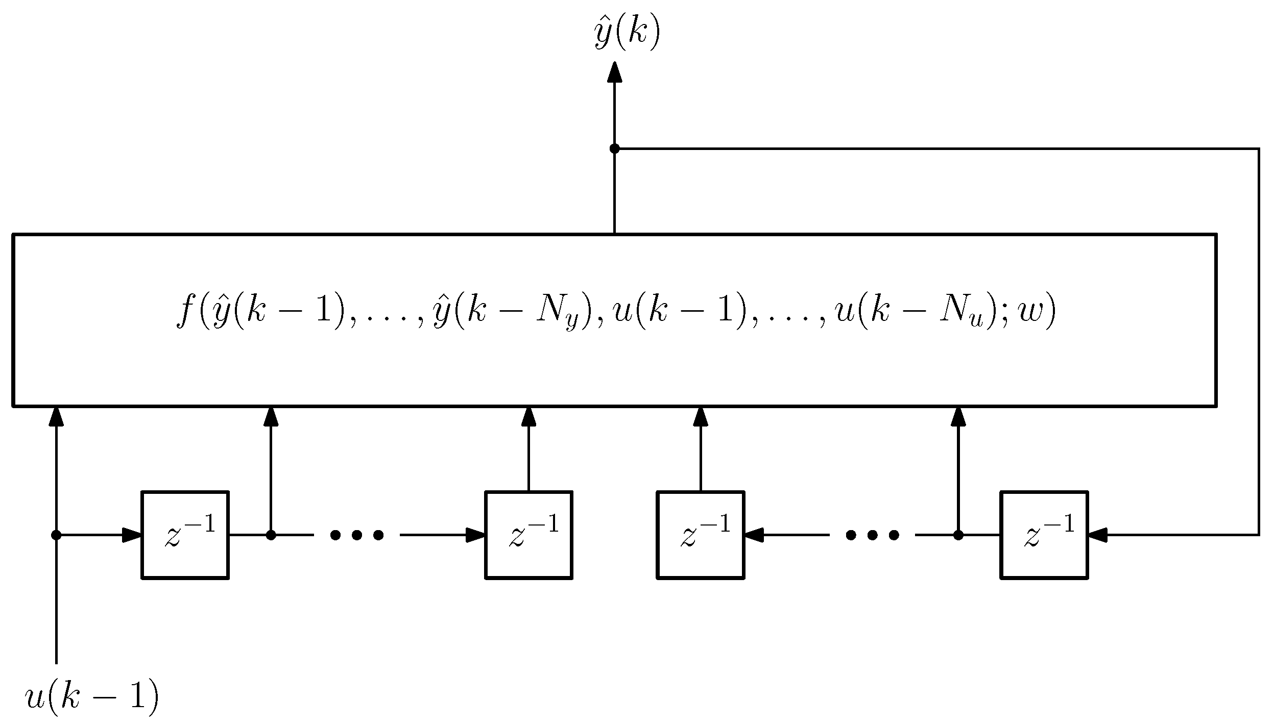
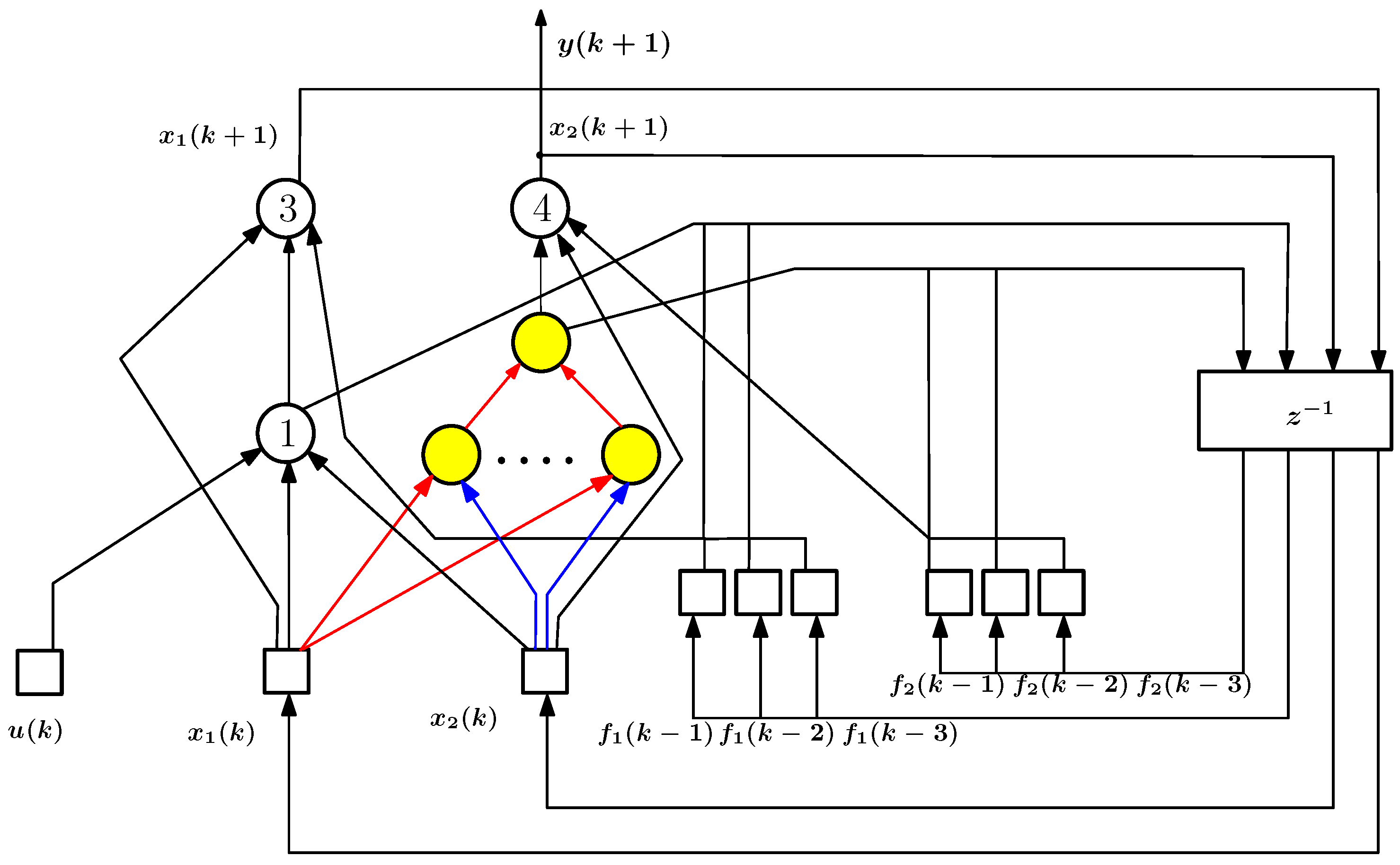
Aircraft flight dynamics is described in general by a nonlinear model. In neural networks, the NARX (Nonlinear AutoRegression with eXogenous inputs) network is often used as such a model. An extension of the NARX model is NARMAX (Nonlinear AutoRegression with Moving Average and eXogenous inputs), which allows explicitly taking into account random external influences on the system when training the network. Both of these models [2,32,46,63] are recurrent neural networks in the considered case. Next, as an example of neural network-based nonlinear system identification, we will consider the NARX model, whose structural scheme is shown in Figure 5.

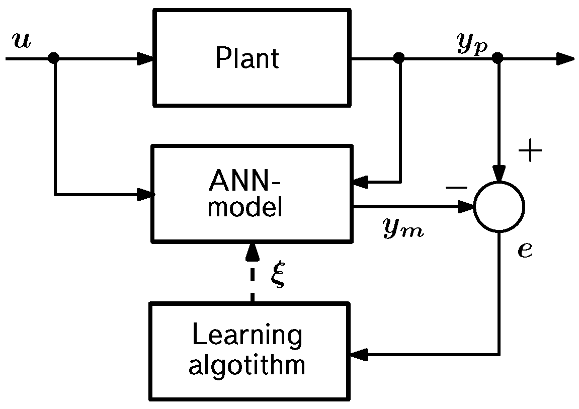
The general scheme of the identification problem-solving is shown in Figure 6, which demonstrates that the same control signal u is fed to the input of both the control object (plant) and the formed ANN model of the object (NARX in our case). The object responds to this control signal by producing an output value $y_p$, which is compared with the ANN model output $y_m$. In addition, the object output $y_p$ is also used as additional information in the ANN model generation process. The result of comparing $y_p$ and $y_m$ equals $\epsilon$. This is the error with which the ANN model reproduces the behavior of the object at a given instant of time and at given values of adjustable parameters, i.e., synaptic weights of the neural network. The learning algorithm takes the $\epsilon$ error as input and generates corrective actions $\xi$ that change the weights to reduce the $\epsilon$ error.

The NARX model, which we use to solve the identification problem, operating in discrete time, realizes a dynamic mapping described by a difference equation of the following kind:

$$\widehat{y}\left(k\right)=f(\widehat{y}(k-1),\widehat{y}(k-2),\dots ,\widehat{y}(k-N_y),u(k-1),u(k-2),\dots ,u(k-N_u);w),$$

(29)

where the value of the output signal $\widehat{y}\left(k\right)$ for a given time instant k is computed based on the values $\widehat{y}(k-1),\widehat{y}(k-2),\dots ,\widehat{y}(k-N_y)$ of this signal for a sequence of previous time instants, as well as the values of the input (control) signal $u(k-1),u(k-2),\dots ,u(k-N_u)$ external to the NARX model. In the general case, the length of the prehistory by outputs and controls may not coincide, i.e., $N_y\ne N_u$. In (29), w represents the set of adjustable parameters of the NARX model (synaptic weights). A convenient way to implement the NARX model is to use a multilayer feedforward network of multiperceptron type to approximate the mapping $f(·)$ in the relation (29) and time delay lines (TDL) to obtain the values of $\widehat{y}(k-1),\widehat{y}(k-2),\dots ,\widehat{y}(k-N_y)$ and $u(k-1),u(k-2),\dots ,u(k-N_u)$. In this case, the NARX network contains one hidden layer, as well as TDL elements for input and output signals. The hidden layer neurons are sigmoidal (linear input part and hyperbolic tangent as an activation function); the output layer neurons are linear, i.e., in addition to the linear input part, they also contain a linear activation function. Variable parameters in training the network are weights of its connections; the RTRL (Real-Time Recurrent Learning) algorithm was used for training. The hyperparameters in the NARX network training task are the number of neurons in the hidden layer, the number of cells in the TDL (delays), and the maximum allowable number of iterations of the training process. The number of neurons in the hidden layer and the number of delays are adjusted experimentally. In particular, the results shown in Figure 7 are obtained for 15 neurons in the hidden layer (the range of variation of this parameter from 10 to 20 was investigated) and for two delays in the TDL element (the range of variation of this parameter from 1 to 10 was investigated). Each iteration of the training process, called a training epoch, consists of running through the network all examples from the training set, which contains 2000 examples (time interval of 40 s, sampling step 0.02 s).

The training of the considered ANN model is performed in the standard way [62,63] as a process of minimizing the sum of squares of errors $e\left(w\right)=y\left(w\right)-\widehat{y}\left(w\right)$ over the whole training sequence of length N:

$$E\left(w\right)={\displaystyle \frac{1}{2}}{e}^T\left(w\right)e\left(w\right),e={[e_1,e_2,\dots ,e_N]}^T.$$

(30)

Here, $y\left(w\right)$ represents the output values of the modeled object (they are taken from the training set), and $\widehat{y}\left(w\right)$ is the output estimate obtained by the ANN model for the current value of the set of its adjustable parameters w.

3.2. Example of an Empirical Neural Network Model of Aircraft Motion

As an example, let us consider one of the problems of modeling the motion of controlled dynamical systems that we have solved, namely, the problem of controlling the longitudinal angular motion of a supersonic transport plane (SST) [118,119]. In flight dynamics, such motion is described by a mathematical model of the following form [33,36]:

$$\begin{array}{cc}\hfill \dot{\alpha }& =q-{\displaystyle \frac{\overline{q}S}{mV}}{C}_L(\alpha ,q,{\delta }_e)+{\displaystyle \frac{g}{V}},\hfill \\ \hfill \dot{q}& ={\displaystyle \frac{\overline{q}Sc}{J_y}}{C}_m(\alpha ,q,{\delta }_e),\hfill \\ \hfill T^2{\ddot{\delta }}_e& =-2T\zeta {\dot{\delta }}_e-{\delta }_e+{\delta }_e^{act},\hfill \end{array}$$

(31)

where $\alpha$ is the angle of the attack, deg; q is the pitch angular velocity, deg/s; ${\delta }_e$ is the deflection angle of the elevator, deg; $C_L$ is the lift coefficient; $C_m$ is the pitching moment coefficient; m is the mass of the aircraft, kg; V is the airspeed, m/s; $\overline{q}=\rho V^2/2$ is the airplane dynamic pressure; $\rho$ is the mass air density, kg/m³; g is the acceleration of gravity, m/s²; S is the wing area of the aircraft, m²; c is the mean aerodynamic chord, m; $J_y$ is the pitching moment inertia, kg · m². Dimensionless coefficients $C_L$ and $C_m$ are nonlinear functions of angle of attack; T and $\zeta$ are the time constant and relative damping factor for the elevator actuator; and ${\delta }_e^{act}$ is the command signal value for the elevator actuator limited by $\pm {25}^{\circ }$.

In the model (31), variables $\alpha$, q, ${\delta }_e$, and ${\dot{\delta }}_e$ are aircraft states; variable ${\delta }_e^{act}$ is aircraft control.

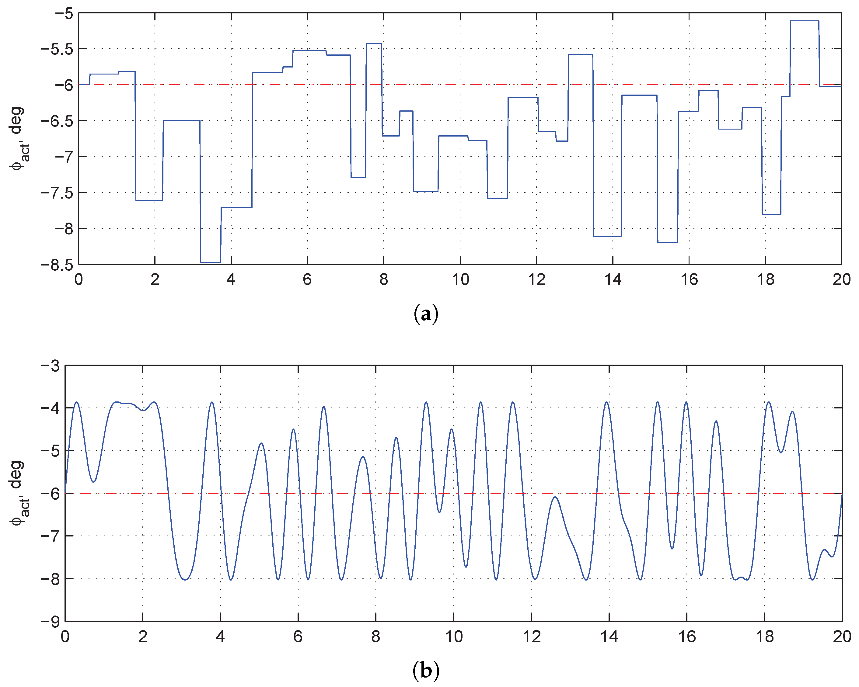
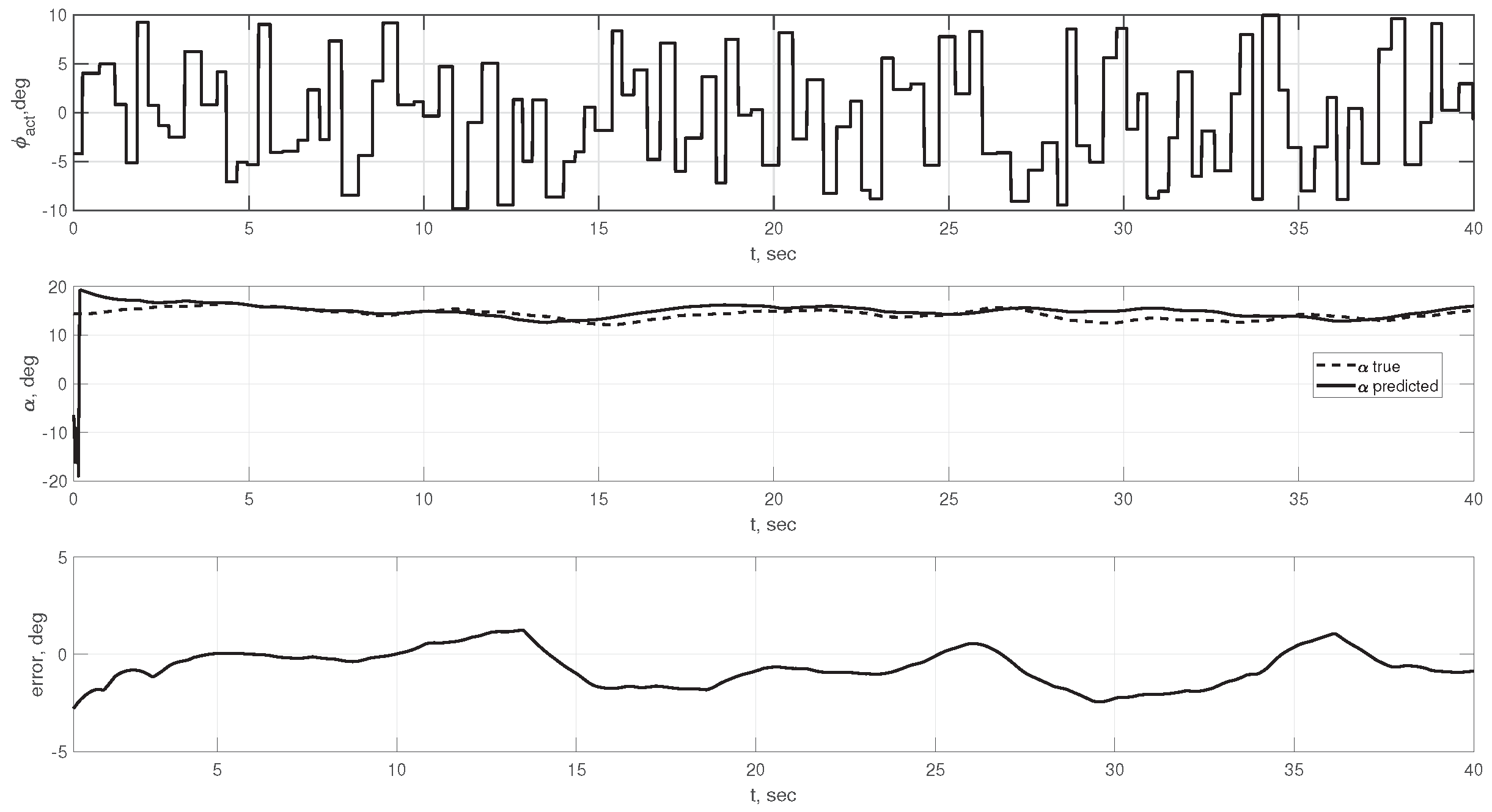
The source data for training of the considered ANN model were generated using a random step signal $u\left(t\right)={\delta }_{\mathrm{in}}\left(t\right)$ fed to the input of the dynamical system. This signal is a sequence of steps with the following parameter values: elevator deflection angle in the range from $-10$ to 10 degrees for a time from 0.25 to 0.5 s. The time step was chosen to be 0.01 s. The total length of the sequence was equal to 40 s. An example of such a signal is presented in the upper part of Figure 7.

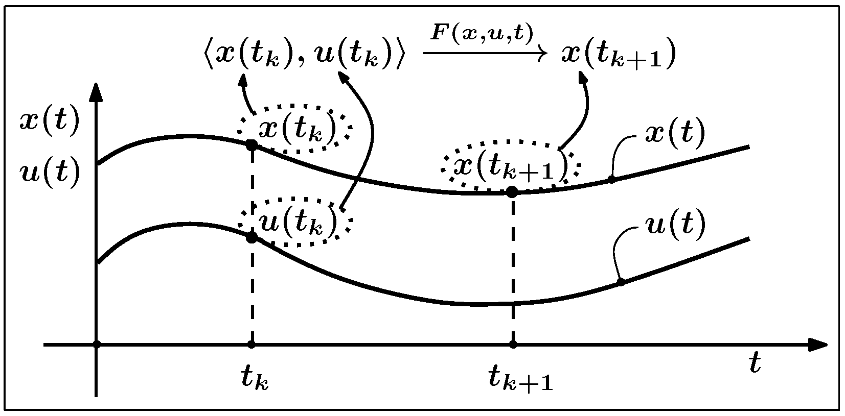
The system under study responds to the input signal $u\left(t\right)$ by changing its state $x\left(t\right)$. The pair $\{t,u(t\left)\right\}$ in this case is the source information for generating a set of training examples. Each of the examples p included in the training set P should show the reaction of the system to some combination $\langle x,u\rangle$. By such a response we mean the state $x\left(t_{k+1}\right)$ to which the system (31) will move from the state $x\left(t_k\right)$ at the value $u\left(t_k\right)$ of the control action (see also Figure 2):

$$\langle x\left(t_k\right),u\left(t_k\right)\rangle \stackrel{F(x,u,t)}{\to }x\left(t_{k+1}\right).$$

Thus, the example p from the training set P will include two parts, namely, the input (this is the pair $\langle x\left(t_k\right),u\left(t_k\right)\rangle$) and the output (this is the response of the system $x\left(t_{k+1}\right)$); see also Figure 2.

To implement the scheme described above, a number of variants with different numbers of neurons in the hidden layer, delays, and training epochs were tried with respect to the NARX network. The results for one of these variants are shown in Figure 7.

As can be seen from Figure 7, the modeling error reaches unacceptable values at some time instants. Different combinations of values for the network and training process parameters did not improve the results. In particular, increasing the delay parameter (i.e., the depth of the prehistory taken into account in (29)) required a sharp increase in the training time. Within the given constraints on computational resources, this requirement could not be met.

It should be noted here that such intensive elevator operation, i.e., sharp and frequent changes in the command signal ${\varphi }_{act}$ of the elevator actuator, is very unlikely in real practice. In other words, we obtain training data “with a large margin” for aircraft operation modes, i.e., under conditions much more severe than they will be in real flight. Nevertheless, these data allow us to understand the limits of the capabilities of ANN models of the black-box type for the considered class of modeling tasks. Our experience in building and using such models for aircraft of various classes shows [120,121,122,123] that the threshold complexity of the flight dynamics problem for such models in most cases is the longitudinal angular motion problem (31) just considered. In more complicated problems, as a rule, it is not possible to obtain acceptable generalization properties from these models.

Within the considered approach, we formed and used ANN models of the black-box type for aircraft of different classes [120,121,122,123,124]. Our experience shows that the threshold complexity of the flight dynamics problem for such models in most cases is the longitudinal angular motion problem (31) just considered. In more complicated problems, as a rule, it is not possible to achieve acceptable generalization properties from these models, i.e., their reasonable accuracy on test data. The same will be true for dynamical systems of other classes similar in complexity level, which is determined by the total number of state and control variables, the ranges of variation in the values of these variables, and the number of samples in each of these ranges.

As noted in the introduction, one possible way to overcome this limitation is to move from purely neural network recurrent models of the black-box type to hybrid ANN models of the gray-box type. These issues are discussed in the next section, which compares empirical and semi-empirical ANN models of controllable dynamical systems. In the same section, two more examples of ANN models of the black-box type are discussed. The results obtained for them are compared with the results for semi-empirical ANN models for the same controlled objects.

4. Semi-Empirical Models of Controlled Dynamical Systems

In this section, as in the previous one, we consider the problem of mathematical and computer modeling of nonlinear controllable dynamical systems operating under numerous and diverse uncertainties, including uncertainties associated with insufficient and inaccurate knowledge about the modeling object and its operating conditions.

As it was shown earlier, empirical ANN models have serious limitations in the complexity level of solved problems. This is due to the high dimensionality of such models, i.e., the significant number of connections in them, which causes the need for numerous training examples. In this regard, there arises the problem of reducing the dimensionality of the created model in such a way that its flexibility does not degrade. One of the possible ways to solve this problem is through the transition to semi-empirical networks that combine the capabilities of theoretical and neural network modeling.

This area has a long history of progress already [49,50,51,52,53,54,55]. The assumptions for it were as follows. There is a situation when, using only available data on the behavior of the object under study, we cannot obtain a model of the required accuracy. At the same time, quite often we also have at our disposal theoretical knowledge about this object, which in the case of a dynamic system has the form of a system of differential equations. When forming an empirical model, we do not use this knowledge at all. In a situation when this approach fails to meet the requirements for modeling accuracy, a natural question arises: maybe it is necessary to somehow involve the available theoretical knowledge about the object in order to meet these requirements? The answer to this question is hybrid models of the gray box type. Such models can be obtained for both uncontrolled and controlled dynamical systems.

In particular, a field called physics-informed neural networks (PINN) is being actively developed [125,126,127,128,129,130,131,132,133]. This field is mainly focused on modeling uncontrolled dynamical systems for which the available theoretical knowledge is expressed in the form of ordinary differential equations or partial differential equations. Even if the system under consideration contains control variables, it is generally assumed that their form is specified. This approach, despite all its advantages, is of limited use for obtaining models of controllable dynamic systems oriented to the needs of adaptive control systems.

We are developing an alternative variant of the gray box models [56,57,58,59,60,61,123,134,135,136], which we call semi-empirical because of their hybrid nature: They are based on an empirical black-box model (recurrent neural network), as it ensures the model’s adaptability. At the same time, knowledge about the modeled object, which takes the form of a system of ordinary differential equations, is embedded in such a network. This approach, as will be demonstrated below, allows us to drastically reduce the size of the resulting model and substantially raise the complexity threshold of the modeling and identification problems to be solved.

4.1. Semi-Empirical Model Development

The formation of semi-empirical ANN models consists of the following steps [56,57,58]:

1.

Obtaining a theoretical continuous-time model for the dynamical system under study and collecting available experimental data on the behavior of this system;

2.

Accuracy assessment for the theoretical model of the dynamical system on the available data; if its accuracy is insufficient, hypothesizing about the reasons for it and possible ways to eliminate them;

3.

Transformation of the source continuous-time model into a discrete-time model;

4.

Formation of neural network representation for the obtained discrete-time model;

5.

Training of the neural network model;

6.

Evaluation of the accuracy for the trained neural network model;

7.

Correction, in case of insufficient accuracy, of the neural network model by making structural changes in it.

Let us assume that the source theoretical model of the object under consideration has already been obtained in one way or another. A typical situation is when such a model is a system of differential equations. In particular, this is the case in the flight dynamics of aircraft. Since this is a continuous-time model and its implementation is carried out in a digital environment, the first step is to discretize the source model. This operation is necessary to obtain a dynamical system with discrete time, for which the corresponding recurrent neural network is built. The choice of the discretization method [42,43,44,45] plays an important role since the consequences of this choice affect the stability of the resulting discrete-time model. The algorithmic basis for discretization of continuous-time models is numerical methods for solving ordinary differential equations (ODE) combined with experience in solving various kinds of such problems. The transition to discrete time in the problem (2) can be based on almost any of the known methods of numerical integration for ODE systems [42,43,44,45]. As an example, to compare semi-empirical models with empirical ones, we will use two explicit difference schemes, namely the 1st order Euler scheme and the 4th order Adams scheme:

• Euler difference scheme:

  $$\mathbf{x}(k+1)=\mathbf{x}\left(k\right)+\Delta t·\mathbf{f}\left(k\right);$$

  (32)
• Adams difference scheme:

  $$\mathbf{x}(k+1)=\mathbf{x}\left(k\right)+{\displaystyle \frac{1}{24}}\Delta t\left[55·\mathbf{f}\left(k\right)-59·\mathbf{f}(k-1)+37·\mathbf{f}(k-2)-9·\mathbf{f}(k-3)\right].$$

  (33)

In (32) and (33), the following notations are used:

$$\begin{array}{c}\mathbf{x}\left(k\right)=\mathbf{x}\left(t_k\right),\mathbf{f}\left(k\right)=\mathbf{f}(t_k,\mathbf{x}\left(k\right)),\\ t=t_0,t_1,\dots ,t_k,\dots ,t_N,\Delta t=t_k-t_{k-1}.\end{array}$$

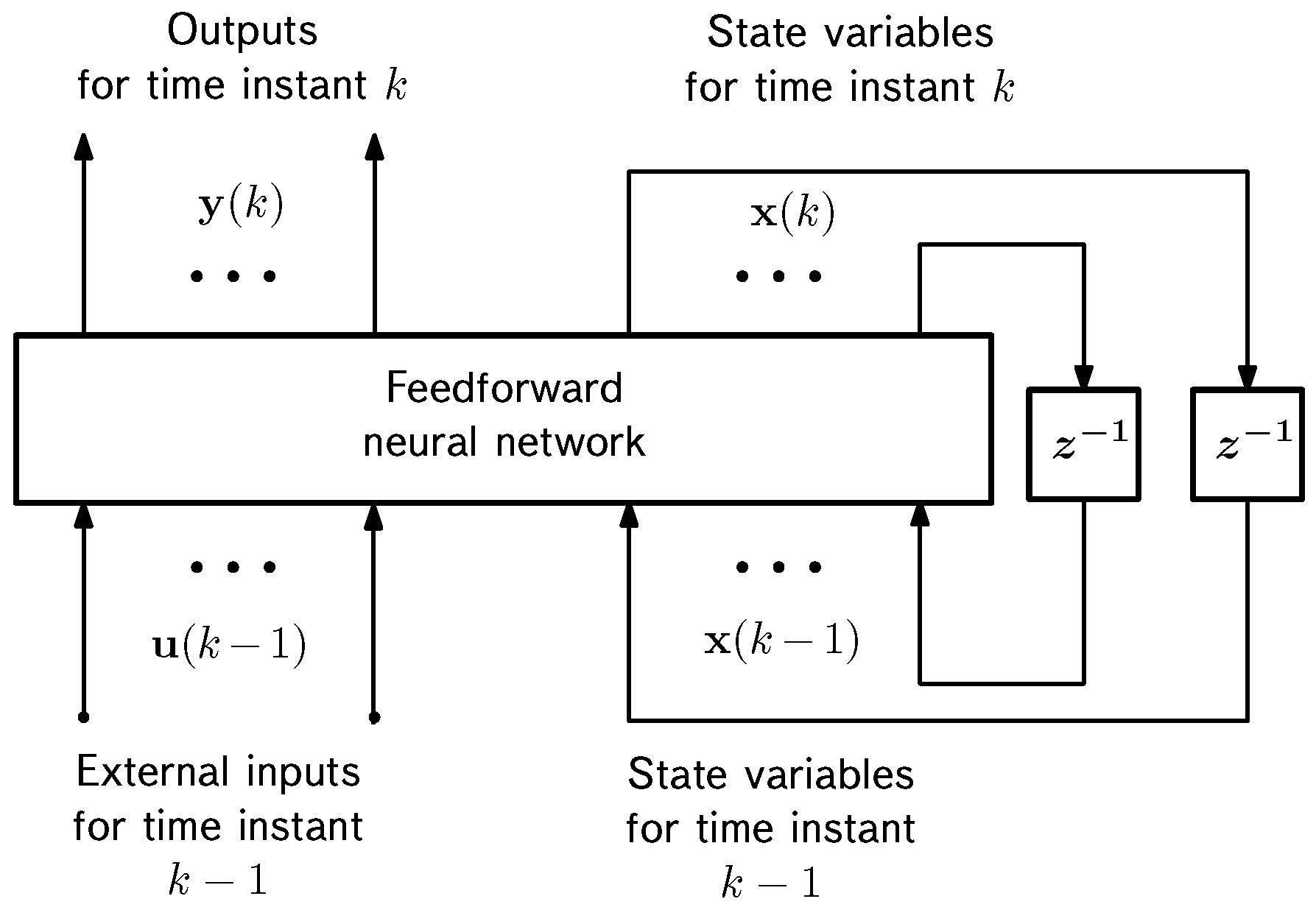
It is well known that any mathematical model or algorithm can be represented as a network structure. In the case under consideration, related to ordinary differential equations and algorithms for their numerical integration, this structure has a recurrent form similar to the structure of recurrent neural networks. Obviously, different source continuous-time models will lead to a variety of recurrent networks. The problem of unification of such networks arises, whose solution avoids the need to build for each of the networks its own training algorithm. Such a solution was proposed in [51,53]. It is based on reducing the original model to some “canonical” form. This problem can be solved for any recurrent neural network, and its final canonical form will be the minimum complexity model in the state space. 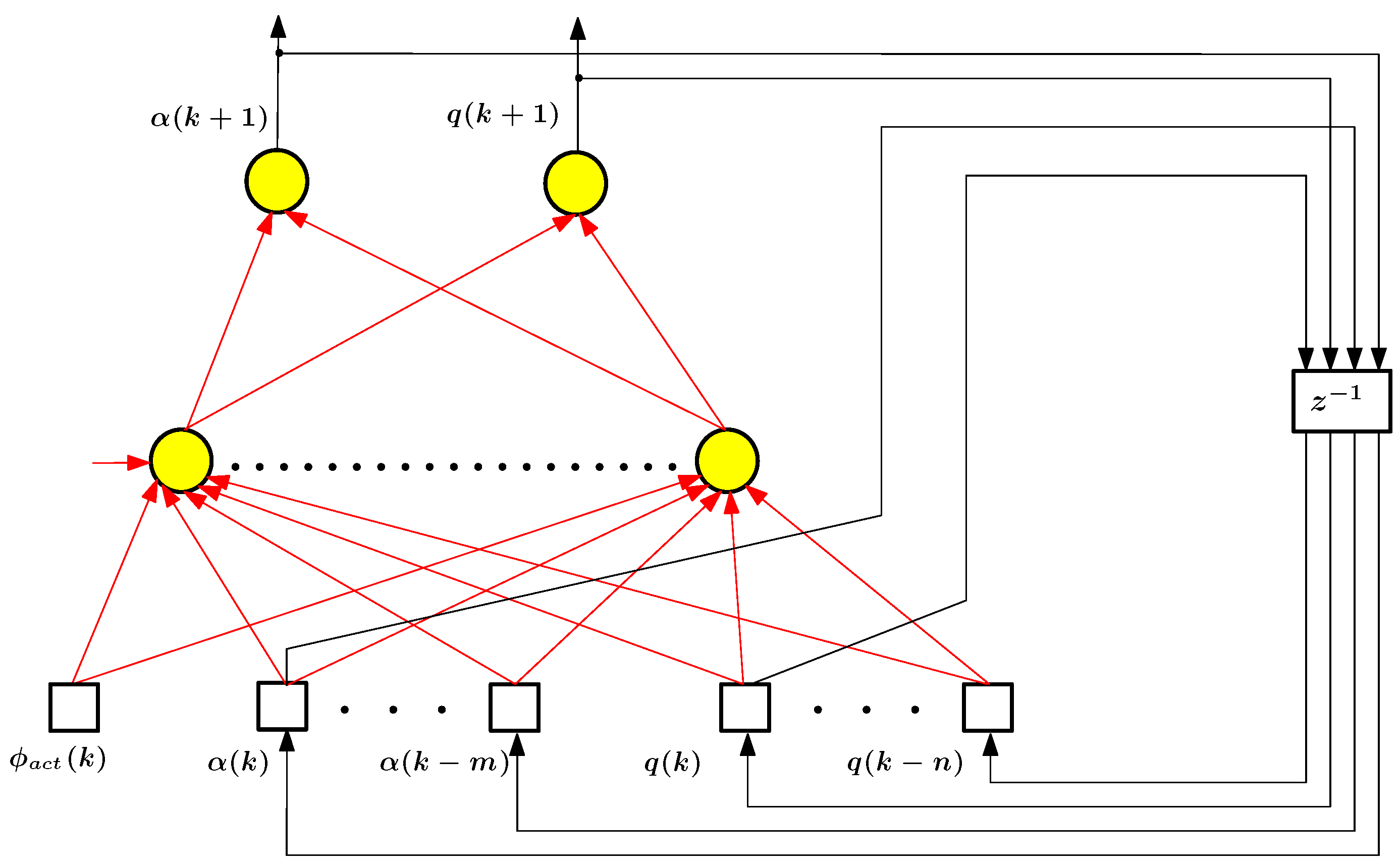The canonical form of the recurrent neural network is given in Figure 8, which shows that the core of this representation is a feedforward neural network, and all feedbacks available in the model are external to the core of this model and contain only unit delays.

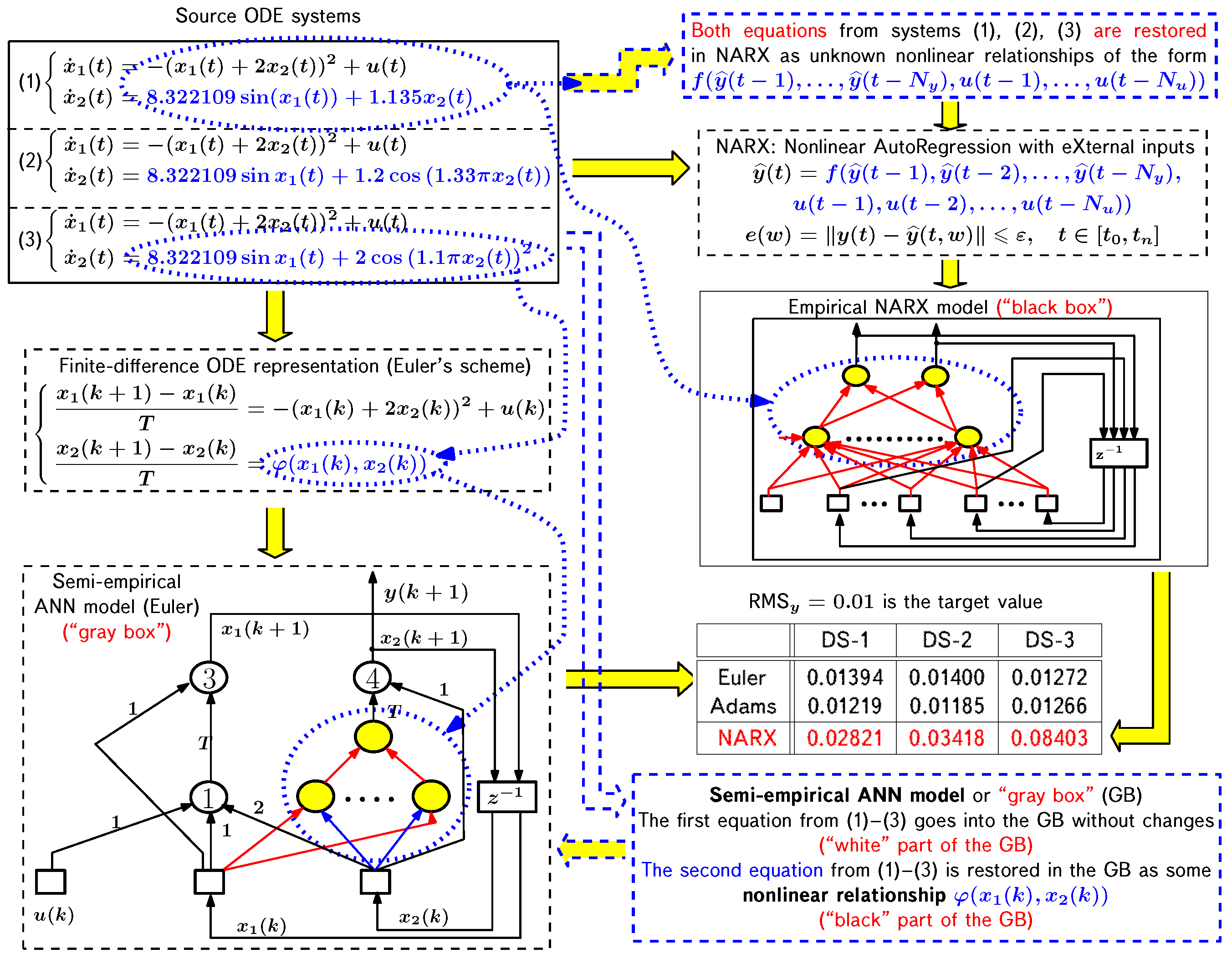
4.2. Semi-Empirical Model of a Simple Dynamical System

In order to compare the capabilities of the empirical and semi-empirical models, we consider two examples. The first one involves a dynamical system described by the following equations:

$$\begin{array}{cc}\hfill {\dot{x}}_1\left(t\right)& =-{(x_1\left(t\right)+2x_2\left(t\right))}^2+u\left(t\right),\hfill \end{array}$$

(34)

$$\begin{array}{cc}\hfill {\dot{x}}_2\left(t\right)& =8.322109\sin \left(x_1\left(t\right)\right)+1.135x_2\left(t\right).\hfill \end{array}$$

(35)

The dynamical system defined by these relations uses part of the example given in [52] as a prototype. This example is not a model of any particular system; it is purely formal (in [52] it is referred to as “a didactive example”). The purpose of the system (34), (35) is to illustrate the procedure of semi-empirical model formation, as well as its superiority over a purely empirical neural network model in the form of the NARX network.

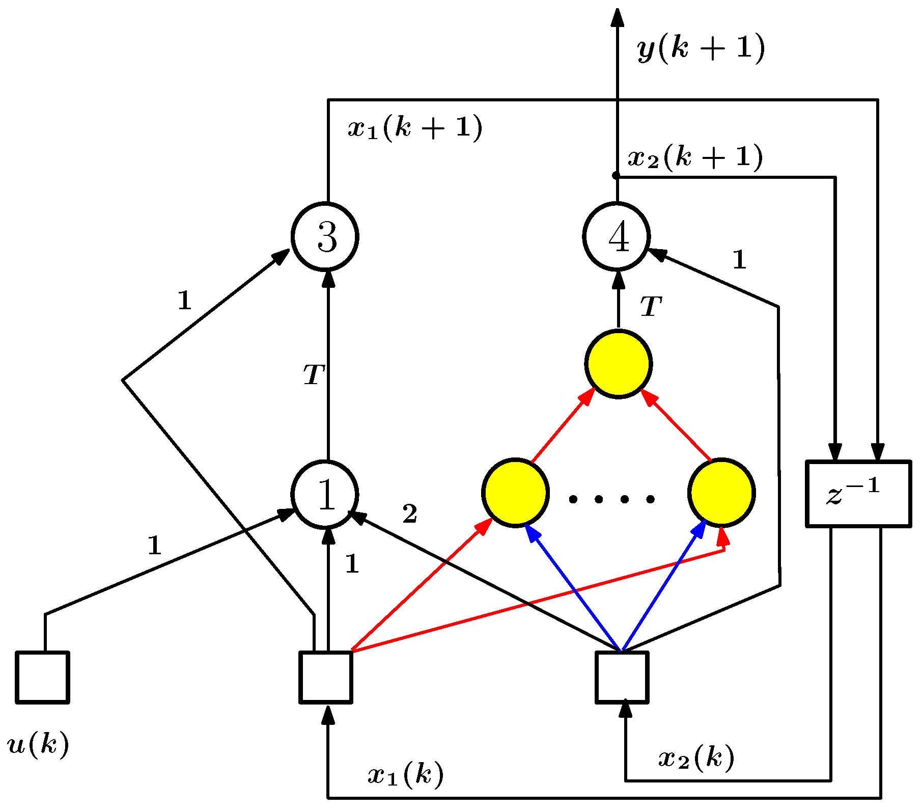
In problems (34) and (35), the adopted discretization schemes allow us to obtain the canonical representation of the network either immediately (for the explicit Euler scheme (32), Figure 9) or after minor adjustments to the initial non-canonical version (for the explicit Adams scheme (33), Figure 10). Some graphical simplification is introduced in Figure 10 in order not to clutter this figure with redundant elements. Namely, the simplified form shows the formation of the Adams scheme from the values of $\mathbf{f}\left(k\right)$, $\mathbf{f}(k-1)$, $\mathbf{f}(k-2)$, and $\mathbf{f}(k-3)$, which are vector functions of the right-hand sides of the equations of motion. Detailed information about the order of formation of this scheme can be obtained from the relation (33) describing it.

Equations (34) and (35) will be used to obtain training and test data in the manner described above. Once these data are obtained, they are used to form a model of the system under consideration, which will be either empirical (black box) or semi-empirical (gray box). In the case of the black-box type model (this is the NARX network), it is assumed that the kinds of both relations (34) and (35) are unknown to us (see Figure 11). For the gray-box model, we will assume that only the kind of relation (35) is unknown, while Equation (34) represents the available theoretical knowledge about the dynamical system under consideration. In such a situation, we deal with a source model of this kind:

$$\begin{array}{c}\hfill \begin{array}{cc}\hfill {\dot{x}}_1\left(t\right)& =-{(x_1\left(t\right)+2x_2\left(t\right))}^2+u\left(t\right),\hfill \\ \hfill {\dot{x}}_2\left(t\right)& =\phi (x_1\left(t\right),x_2\left(t\right)),\hfill \end{array}\end{array}$$

(36)

where $\phi (x_1\left(t\right),x_2\left(t\right))$ is the unknown relationship that needs to be reconstructed during the training of the grey-box model using the available experimental data on the behavior of the dynamical system under consideration. As mentioned above, the results of the integration of the equations (34) and (35) with given initial conditions, integration step, and control function $u\left(t\right)$ are used as these data.

To obtain a gray-box neural network model, including Equation (34) and the relation corresponding to the unknown second equation in the model under consideration, two steps are required. The first step consists of going from the original continuous-time model, i.e., the differential equations, to the discrete-time model, i.e., the difference equations. For this purpose, we will use two explicit difference schemes, namely the 1st order Euler scheme (32) and the 4th order Adams scheme (33).

We consider a system (36) on a time interval $t\in [0;100]$ with a sampling step $\Delta t=0.025$ s and initial conditions $x_1\left(0\right)=x_2\left(0\right)=0$. The state vector is partially observable: $y\left(t\right)=x_2\left(t\right)$, with additive white noise with root-mean-square (RMS) deviation $\sigma =0.01$ affecting the system output $y\left(t\right)$.

Ideally, when the neural network model reproduces the original system of differential equations (34) and (35), the modeling error will be completely determined by the noise affecting the system output. It follows that the comparison of the modeling error with the noise RMS allows us to estimate the degree of success in solving the modeling problem of the system under consideration, and the given value of the noise RMS can be taken as the target value of the modeling error.

Training was carried out using Matlab for LDDN (Layered Digital Dynamic Networks) networks using the algorithm common for this class of networks [63]. The Levenberg–Marquardt algorithm is used to optimize the network parameters, and the Jacobi matrix is calculated using the RTRL (Real-Time Recurrent Learning) algorithm [46]. The RMS prediction error of the model on the training sample is used as an optimization criterion:

$$RMSE=\sqrt{{\displaystyle \frac{1}{N}}\sum _{i=1}^N{(d_i-y_i)}^2},$$

(37)

where N is the number of training set elements, $d=\{d_1,\dots ,d_N\}$ is the vector of target values of the observed variable (according to the model (34) and (35)), and $y=\{y_1,\dots ,y_N\}$ is the vector of outputs of the neural network model.

In the case under consideration, the kind of relation (35) shows that the recoverable right-hand side of the second equation of this model must be nonlinear and have both state variables, $x_1\left(t\right)$ and $x_2\left(t\right)$, as arguments. In the general case, however, these facts are not known to us. Therefore, we need to make a sequence of hypotheses concerning the kind of right-hand side of the second equation in (36). These hypotheses should be ordered by the complexity of the resulting relation: on which variables it depends and whether this relation will be linear or nonlinear on the selected variables. The reasonableness of this approach is determined by the fact that as the complexity of this relationship increases, the number of connections in the neural network that will reproduce it also increases. According to the well-known result [46,63], the dimensionality of the network (i.e., the number of connections in it) and the dimensionality of the training set (the number of examples in it) are strictly related. Consequently, using more complicated relations for the right-hand side of the second equation in (36) will require a larger number of training examples and, consequently, an increase in the time required to train the model. It is for this reason that one should introduce a sequence of hypotheses regarding the kind of relationship to be recovered and then experimentally determine the lowest complexity relationship that allows for the required modeling accuracy.

In the considered example, we omit all intermediate steps and define the reconstructed relation as a nonlinear function of two variables, $\phi (x_1\left(t\right),x_2\left(t\right))$, which depends on both state variables $x_1\left(t\right)$ and $x_2\left(t\right)$ but does not depend on the control variable $u\left(t\right)$. The structural diagram of the network corresponding to this variant of the ANN model for the Euler discretization scheme is shown in Figure 9; similarly, it can be obtained in the case of the Adams scheme (Figure 10). The accuracy of the obtained model (denoted as DS-1 in Figure 11), estimated by the relation (37), is 0.01394 for the Euler method and 0.01219 for the Adams method, with the target value of this index equal to 0.01.

To compare with the traditional approach, let us demonstrate the results of training the NARX model. The best accuracy of 0.02821 in this example was achieved by a network with three neurons in the hidden layer and five delays in the feedback. From this comparison, we can see the undeniable advantage of the semi-empirical model over the empirical model in terms of achievable solution accuracy: even for Euler’s method, the accuracy is 0.01394 versus 0.02821 for NARX. In the case of Adams’ method, the accuracy is even higher. It is equal to 0.01219, and it is possible to improve the accuracy even further by using more efficient difference schemes.

An analysis similar to the one described above was also performed for two more variants of the considered system (34) and (35), denoted as DS-2 and DS-3 in Figure 11. First, instead of Equation (35), this system uses its complicated version with a mixture of harmonics on the right-hand side:

$${\dot{x}}_2\left(t\right)=8.322109\sin \left(x_1\left(t\right)\right)+0.7cos\left(1.33\pi x_2\left(t\right)\right).$$

(38)

In the second variant, Equation (35) is replaced by a relation that contains a more complex mixture of harmonics than in (38):

$${\dot{x}}_2\left(t\right)=8.322109\sin \left(x_1\left(t\right)\right)+0.7cos{\left(1.33\pi x_2\left(t\right)\right)}^2.$$

(39)

The results of calculations for these variants, including for the NARX model, are presented in Figure 11.

A comparison of the experimental results for all three examples allows us to draw the following conclusions.

The kind of difference scheme used influences the accuracy of modeling. In this regard, the problem of choosing an adequate (the best in the ideal case) discretization scheme for a particular applied problem to be solved arises.

In order to eliminate this kind of influence of the difference scheme on the obtained result, we have proposed and implemented an alternative variant of the formation and training of the semi-empirical model [60]. The essence of this variant is as follows. Section 4.1 demonstrates the sequence of steps performed during semi-empirical modeling. It shows that the transformation of the original continuous-time model into a discrete-time model precedes the formation of a neural network representation for the resulting discrete-time model, as well as its training. This means that if the difference scheme used for discretization is unsuccessful, it must be replaced by another one. It is not excluded that this operation will have to be repeated many times to obtain the desired result. Each such replacement must be accompanied by training of the resulting semi-empirical model, and this requires a significant computational resource consumption. In an alternative variant, training is performed for the source model in continuous time, and only after that is its discretization, necessary for operation in a digital environment, performed. In this case, the algorithm for training the model in continuous time is based on the method of sensitivity functions, long known in automatic control theory [137]. Of course, training a continuous-time model will be more time-consuming than a discrete-time model, but it will only have to be conducted once rather than repeatedly. The final decision as to which training option should be used, discrete or continuous, will depend on how repeatedly the reasonable difference scheme is expected to be selected in the first of these two options.

The second important conclusion is related to the comparison of results for empirical and semi-empirical models. It can be seen that semi-empirical models are many times more accurate than purely empirical ones. At the same time, the gap in modeling accuracy increases with the complexity of the behavior of the system under consideration. In this regard, in those cases where the accuracy obtained from the empirical model is insufficient and there is theoretical knowledge about the modeling object, the transition to a model of a semi-empirical type has a significant effect.

4.3. Semi-Empirical Model of Longitudinal Angular Motion of an Aircraft

The basic idea binding the examples discussed below is as follows. We want to solve not only the problem of system identification, for which we have experimental data showing the input influences on the system and its reactions to these influences, and the model that converts inputs to outputs is a black box. We are more interested in the very important task of system characteristics identification. This is, first of all, the aerodynamic characteristics of the aircraft. If we were able to solve this problem, then, substituting the obtained relations into the equations of motion, we obtain the model of the aircraft as a control object in general. To solve this problem within the framework of the semi-empirical approach, we form a hybrid model of motion, the basis for which is one of the traditional models of flight dynamics in the form of a system of ordinary differential equations. We transform it into a network structure, which includes, as customizable elements, feedforward subnets that implement nonlinear functions describing the corresponding dimensionless coefficients of aerodynamic forces and moments. All other elements of the mentioned network structure, which do not coincide with the subnets for the aerodynamic coefficients, obtain the corresponding numerical values of the connection weights from the source motion model in the form of ODEs, after which they are frozen. Thus, we obtain a gray-box type model, which, unlike black-box type models, has significantly fewer adjustable parameters, which greatly simplifies the process of training the model being formed.

The second of two examples that demonstrate the potential of a semi-empirical approach to modeling and identifying controllable dynamical systems involves the longitudinal angular motion of an airplane. We have obtained results that allow us to assess how effective this approach would be in comparison with empirical ANN models (NARX-type recurrent networks).

The theoretical model of aircraft motion is usually a system of first-order ordinary differential equations in normal form [33,34,35]. For example, to describe the full angular motion of an aircraft with pitch, yaw, and roll control, a system of 14 such equations is used, which in general form looks as follows:

$$\dot{x}=f(x,u,t),$$

(40)

where $x=(\phi ,\psi ,\theta ,p,r,q,\alpha ,\beta ,{\delta }_r,{\delta }_e,{\delta }_a,{\dot{\delta }}_r,{\dot{\delta }}_e,$ and ${\dot{\delta }}_a)$ are state variables, and $u=({\delta }_{e_{act}},{\delta }_{a_{act}},$ and ${\delta }_{r_{act}})$ are controls. Here, $\phi$, $\psi$, and $\theta$ are roll, yaw and pitch angles; p, r, and q are roll, yaw, and pitch angular rates; $\alpha$ and $\beta$ are angle of attack and sideslip; ${\delta }_r$, ${\delta }_e$, ${\delta }_a$, ${\dot{\delta }}_r$, ${\dot{\delta }}_e$, and ${\dot{\delta }}_a$ are angles of deflection and angular rates for rudder, elevator, and ailerons; ${\delta }_{e_{act}}$, ${\delta }_{a_{act}}$, and ${\delta }_{r_{act}}$ are command signals of actuators for elevator, rudder and ailerons.

The right-hand sides of the equations in the model (40) contain the following dimensionless coefficients of aerodynamic forces and moments:

$$\begin{array}{cc}\hfill C_D(\alpha ,\beta ,{\delta }_e,q),& C_L(\alpha ,\beta ,{\delta }_e,q),C_y(\alpha ,\beta ,{\delta }_r,{\delta }_a,p,r),\hfill \\ \hfill C_l(\alpha ,\beta ,{\delta }_e,{\delta }_r,{\delta }_a,p,r),& C_n(\alpha ,\beta ,{\delta }_e,{\delta }_r,{\delta }_a,p,r),C_m(\alpha ,\beta ,{\delta }_e,q).\hfill \end{array}$$

(41)

It is the incomplete and inaccurate knowledge of the nonlinear functions (41) that is the main source of uncertainties that make it very difficult to obtain motion models of the kind (40).

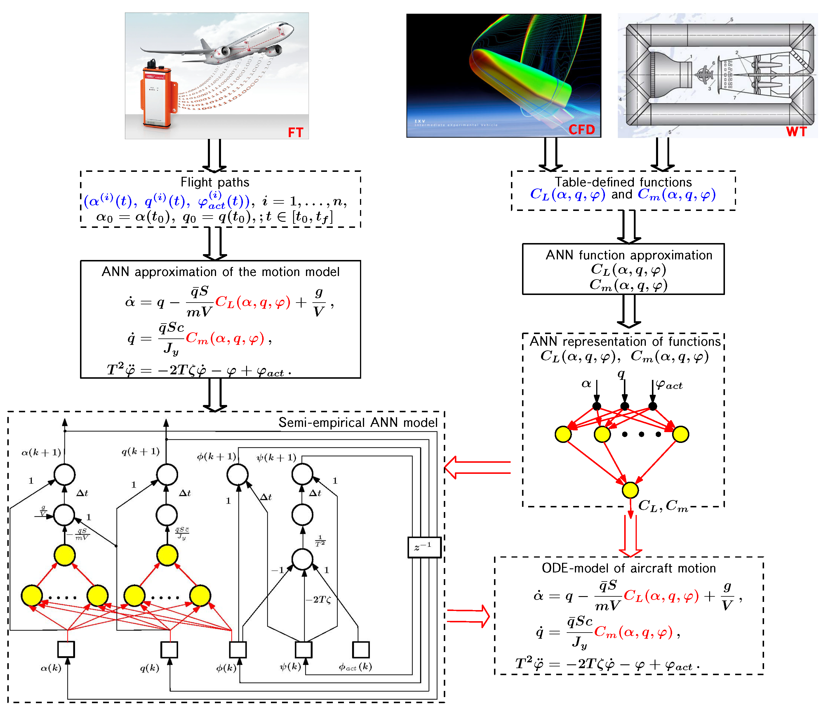
There are two approaches to the formation of dependencies (41): direct and indirect. Let us illustrate the relationship between these two approaches with the example of the modeling problem for longitudinal angular motion of an airplane and identification of the lift force and pitching moment coefficients (see Figure 12).

In the previous example, the model (34), (35) served as sources of training and test data for obtaining neural network models. Similarly, we will use as such a source the model (31) traditional for aircraft flight dynamics [33,34,35], which we introduced earlier in the section on empirical ANN models of motion. As an example of a specific modeling object, we considered a maneuverable F-16 aircraft, the source data for which were taken from [111]. A computational experiment with the model (31) was conducted for a time interval $t\in [0;20]$ sec with a sampling step $\Delta t=0.02$ sec for the partially observed state vector $y\left(t\right)={[\alpha \left(t\right);{\omega }_z\left(t\right)]}^T$, with additive white noise with standard deviation $\sigma =0.01$ affecting the output of the $y\left(t\right)$ system.

This motion model can be used in its original form, i.e., as a system of ordinary differential equations, or as a semi-empirical neural network model built based on these equations. In the first case, it is required to somehow specify the functions $C_L(\alpha ,\beta ,{\delta }_e,q)$ and $C_m(\alpha ,\beta ,{\delta }_e,q)$, which are included in the right-hand sides of the equations (31). In the second case, these functions are included as separate modules in a gray-box type neural network. These functions can be represented in various ways, including kind of feedforward neural networks. The direct and indirect approaches mentioned above differ in the kind of available source data and the way of obtaining the required functions.

In the direct approach, we have data obtained from wind tunnel tests or computational fluid dynamics methods. The results obtained by these techniques have the kind of tabulated functions (41) that serve as a source of both training and test data. In this case, a separate feedforward neural network is formed for each of the aerodynamic coefficients. These networks, as separate functions, can then be inserted into the appropriate places in a model (40) or similar, after which this model can be used in the traditional way as a system of differential equations. An example of such a substitution can be seen in Figure 12.

In the indirect approach, as seen in Figure 12, the input data are state and control variables obtained as functions of time during a flight or computer experiment (as in the previous example). Thus, unlike the direct approach, there are no tabulated functions (41) at our disposal. We have only data characterizing the behavior of our object under given conditions, which is influenced by the values of aerodynamic forces and moments. If all other factors affecting the behavior of the aircraft are fixed, then in this case it is possible to set and solve the problem of identification for aerodynamic coefficients from the above-listed experimental data. It has already been mentioned above that neural network models of the semi-empirical type can solve this problem. Figure 12 shows how such a model looks as applied to the longitudinal angular motion of an aircraft.

It should be emphasized that purely empirical models, in particular the recurrent network of the traditional kind, allow us to solve only the problem of system identification, i.e., they allow us to obtain a model of the control object as a whole. However, no less important is also the problem of identifying the characteristics of the object under consideration, for example, the coefficients of aerodynamic forces and moments in the case of an aircraft. Models of the black-box type do not provide an opportunity to solve problems of this kind. At the same time, models of the gray box type, i.e., semi-empirical models, have such a possibility. They allow for solving both the problem of system identification and the problem of characteristic identification.

This fact is of great importance, since the task of identifying the aerodynamic characteristics of an aircraft from experimental data is one of the most important for flight dynamics and control. The approach to solving this problem based on semi-empirical neural network modeling differs significantly from the traditional one.

Namely, the traditional approach is based on the linearization of functions (41) using their Taylor series expansion with terms not higher than the first order. In this case, the restoring object in the identification problem is the expansion coefficients, which include the derivatives $C_{L_{\alpha }}=\partial C_L/\partial \alpha$, $C_{m_{\alpha }}=\partial C_m/\partial \alpha$ etc. Moreover, this operation is performed “at a point”, i.e., for a particular combination of arguments of these functions and not for the whole area of their definition.

At the same time, the semi-empirical approach recovers nonlinear functions of several arguments—$C_L,C_D,C_y,p,r,$ and q—as holistic objects in the whole range of changes in the values of their arguments. As can be seen from Figure 12, these functions are localized inside the semi-empirical model (they are highlighted in Figure 12). Each of them has its own feedforward network. The training algorithm of this model selects the values of the connection weights of these networks. At the same time, the weights of other connections obtained from its theoretical part are frozen. After the training process is completed, the ANN modules realizing the functions (41) can be extracted from the semi-empirical model and, if necessary, placed as ordinary functions in the model represented by the differential equations of motion. In particular, as shown in Figure 12, the ANN modules for the functions $C_L(\alpha ,q,\phi )$ and $C_m(\alpha ,q,\phi )$ can be used in the right-hand sides of the equations describing the longitudinal angular motion of the airplane.

In some cases, for the restored functions $C_L(\alpha ,\beta ,{\delta }_e,q)$, $C_m(\alpha ,{\delta }_e,q)$, etc., we need to find the values of their partial derivatives, for example, $C_{L_{\alpha }}={\displaystyle \frac{\partial C_L}{\partial \alpha }}$, $C_{l_{\beta }}={\displaystyle \frac{\partial C_l}{\partial \beta }}$, $C_{m_{\alpha }}={\displaystyle \frac{\partial C_m}{\partial \alpha }}$, etc. For example, the variation of the partial derivative of the pitching moment coefficient with the angle of attack provides useful information for flight dynamics and control specialists.

If necessary, the partial derivatives of the functions $C_D(·)$, $C_L(·)$, …, $C_m(·)$, given in the form of ANN modules, can be computed using an algorithm similar to the error backpropagation algorithm used to train the ANN model as a whole.

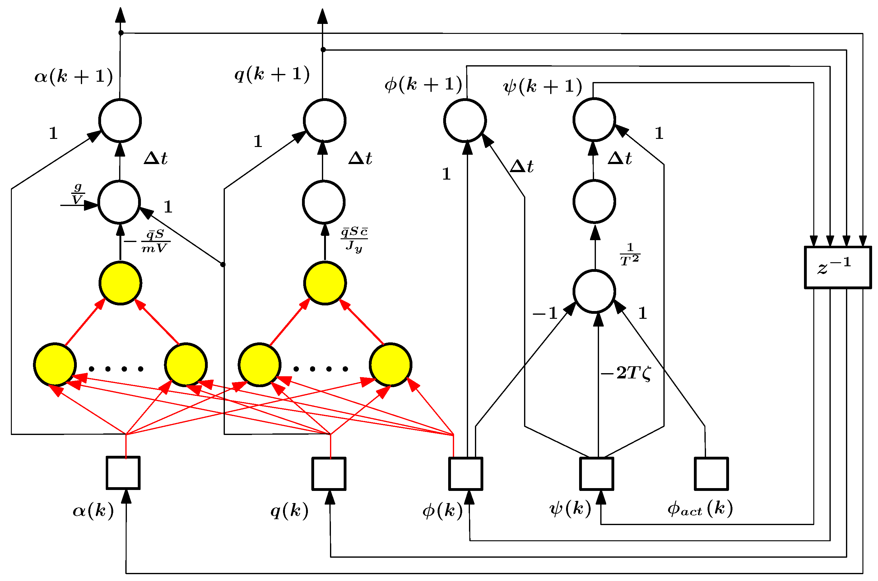
Applying to (31) the above-mentioned procedure of forming a semi-empirical ANN model leads to the structure shown in Figure 13 (it is based on the Euler discretization scheme). A similar structure for the case of a fully empirical model (NARX) corresponding to the same problem (31) is shown in Figure 14. For the case of the Adams scheme, a semi-empirical model can be constructed in a manner similar to that shown in Figure 11 for the previous example.

As it was mentioned earlier, one of the critical issues arising in the formation of empirical and semi-empirical ANN models is obtaining a training set that provides an adequate representation of the peculiarities of the behavior of the modeled system. This formation is carried out by developing an appropriate test control action on the modeled object and evaluating the object’s response to this action.

As in the previous example, we will use the RMS of additive noise acting on the system output as the target value of the modeling error.

The model under consideration is trained on the sample $\left\{\langle {\alpha }_i,q_i,{\varphi }_i,{\dot{\varphi }}_i,{\dot{\varphi }}_i\rangle \right\},i=1,\dots ,N$, obtained using the source model (31), steady state straight line horizontal flight as the reference mode, and a polyharmonic excitation signal. It was performed in Matlab for networks in the form of LDDN (Layered Digital Dynamic Networks) using the Levenberg–Marquardt algorithm and the MSE criterion. The Jacobi matrix is calculated using the RTRL (Real-Time Recurrent Learning) algorithm [46].

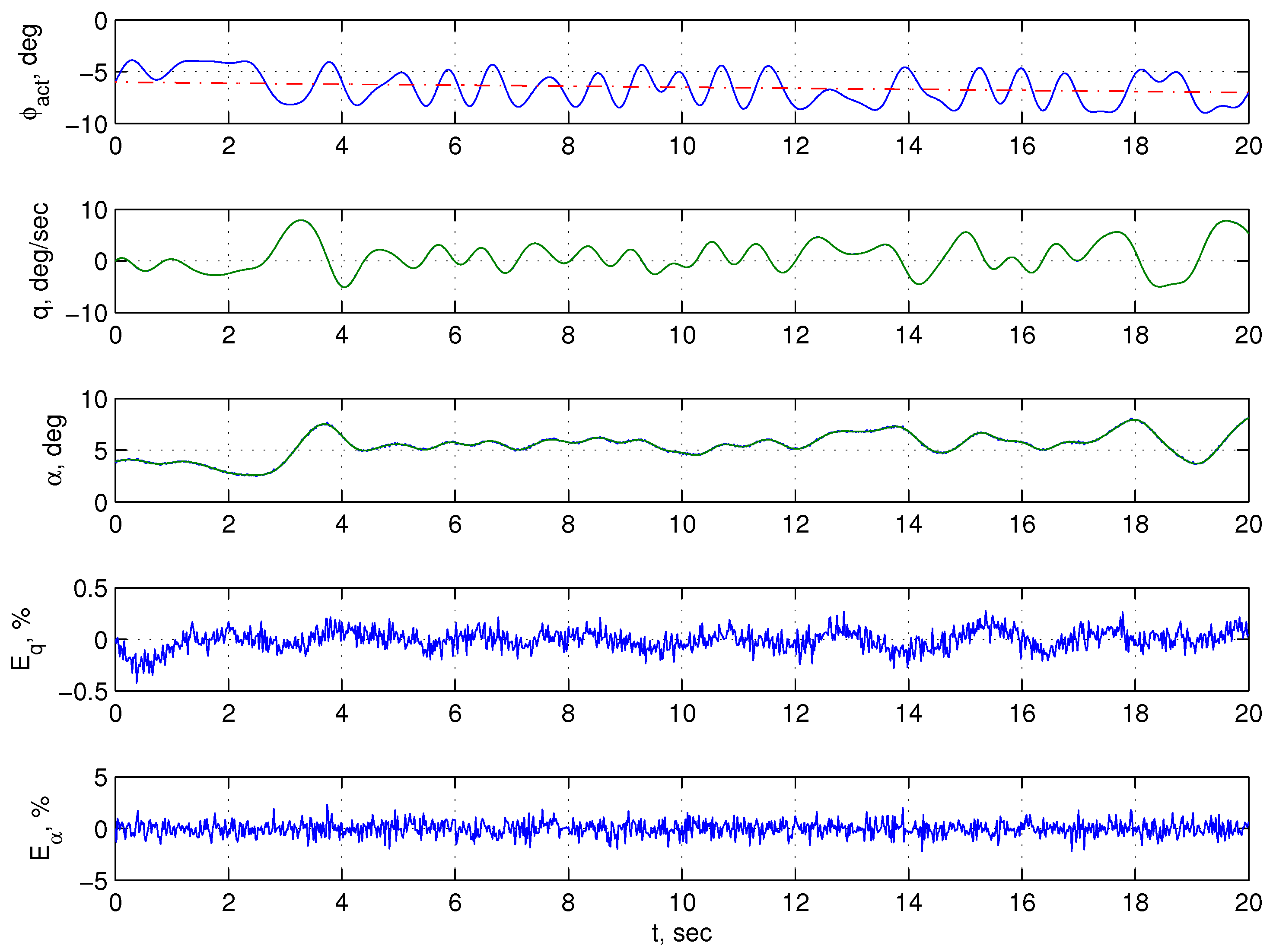
As follows from the results shown in Figure 15, the generated semi-empirical model has a very high accuracy. The pitch rate error is within $\pm 0.3$%, and the angle of attack error is within $\pm 2$%. Since the uncertainty factors in the source model are only the relationships for the aerodynamic force and moment coefficients, these results indicate a successful solution not only to the problem of system identification but also to the problem of characteristic identification, i.e., the lift force and pitching moment coefficients in the problem under consideration.

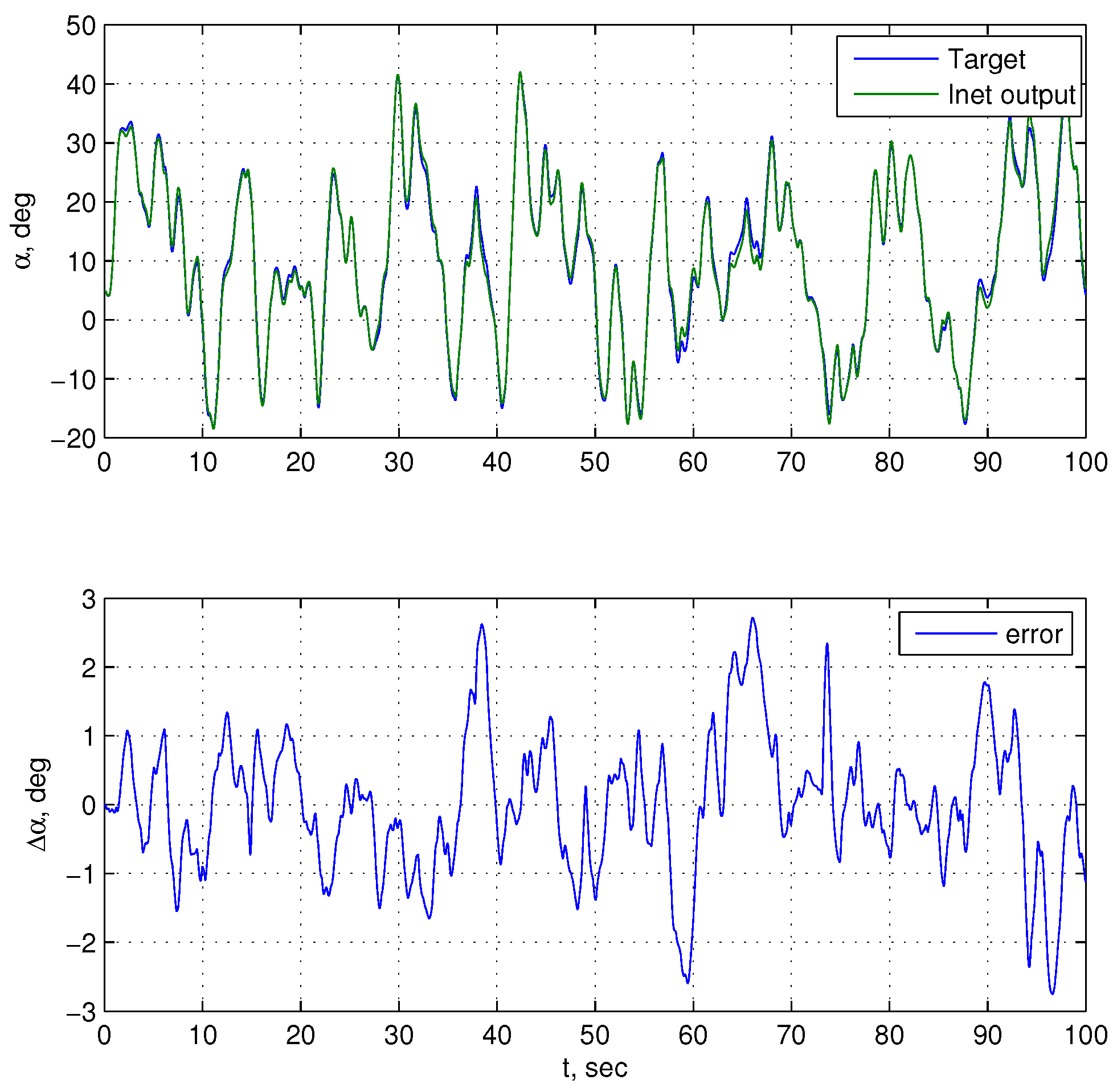
Let us compare the results obtained for the semi-empirical and empirical motion models corresponding to the system (31). For the empirical ANN model of NARX type, the results are presented in Figure 16. A comparison of the results for these two variants of ANN models of longitudinal angular motion of the airplane allows us to draw the following conclusions. The values of the current modeling error in angle of attack lie within $\pm 0.5$ deg for the semi-empirical model and within $\pm 2.5$ deg for the NARX model. Typical RMS error values are ${\mathrm{RMS}}_{\alpha }=0.05$ deg, ${\mathrm{RMS}}_q=0.1$ deg/s for the semi-empirical model, and ${\mathrm{RMS}}_{\alpha }=1.3$ deg, ${\mathrm{RMS}}_q=2.7$ deg/s for the empirical model. Thus, as in the previous example, the semi-empirical model has an undeniable advantage in accuracy over the empirical model.

As noted above, the source of uncertainty in the motion model (31) is the functions $C_L(\alpha ,{\delta }_e)$ and $C_m(\alpha ,{\delta }_e)$ which describe the dependence of the lift coefficient and pitching moment coefficient on the angle of attack $\alpha$ and elevator deflection angle ${\delta }_e$. These dependencies have a complicated character, especially for a maneuverable aircraft. As an example, the dependence $C_m(\alpha ,{\delta }_e)$ for an F-16 airplane, plotted using data from the [111], is shown in Figure 17a. We see that the value of the coefficient $C_m$ is subject to frequent and significant changes when the parameters $\alpha$ and ${\delta }_e$ are varied over wide ranges. Even more significantly, the derivative of this coefficient, especially $\partial C_m/\partial \alpha$, repeatedly changes sign since for values of the angle of attack at which this derivative is positive, the control object is unstable. It follows that a nonlinear function of several arguments, $C_m(\alpha ,{\delta }_e)$, must be reconstructed with very high accuracy to avoid incorrect values of its derivative if possible. The semi-empirical approach allows us to cope with this problem, as can be seen from Figure 17b for the considered example.

The above results of the problem (31) clearly demonstrate the capabilities of the semi-empirical approach. It provides a model of aircraft motion that is considerably more accurate than can be achieved by the empirical approach. In addition, unlike the empirical approach, it is possible to identify the characteristics of the object under consideration. In the case considered, these are the aerodynamic coefficients $C_L$ and $C_m$ as nonlinear functions of several variables.

As already noted above, the problem of modeling the controlled longitudinal angular motion of an airplane is the threshold problem in terms of the complexity of the empirical approach. The semi-empirical approach can be used to form a model of this kind without any significant difficulties while ensuring, as already noted, a much higher level of modeling accuracy.

Our experience shows [134,135,136] that this approach can be used to successfully solve identification problems for objects much more complicated than (31). In particular, the problem (40), (41) and fourteen state variables instead of four in (31), as well as three control variables instead of one. In problems of this kind, it was possible to obtain very high accuracy both for the model of the control object as a whole and for the functions describing all six coefficients of aerodynamic forces and moments. However, to ensure such a result, it was necessary to significantly increase the number of examples in the training set. If in problems of the kind (31) the typical number of examples was ${10}^3$, then in problems of the kind (40), (41), and similar problems, about $5·{10}^5$ is required.

The accuracy of the model to be formed is determined by how precisely the nonlinear functions describing the aerodynamic characteristics of the aircraft are reconstructed, i.e., how effectively the problem of identifying these characteristics is solved. To obtain an answer to this question, we can extract from the semi-empirical model the ANN modules corresponding to the restored functions for $C_L$, $C_Y$, $C_l$, $C_n$, and $C_m$, and then compare the values they produce with the experimentally available data from [111]. In doing so, we can obtain the mean square error values of the derivation of each of the functions $C_L$, $C_Y$, $C_l$, $C_n$, and $C_m$ by the corresponding ANN module. In the experiments performed, these values are as follows: ${\mathrm{MSE}}_{C_L}=9.2759·{10}^{-4}$, ${\mathrm{MSE}}_{C_Y}=5.4257·{10}^{-4}$, ${\mathrm{MSE}}_{C_l}=2.1496·{10}^{-5}$, ${\mathrm{MSE}}_{C_n}=1.3873·{10}^{-5}$, ${\mathrm{MSE}}_{C_m}=1.4952·{10}^{-4}$. 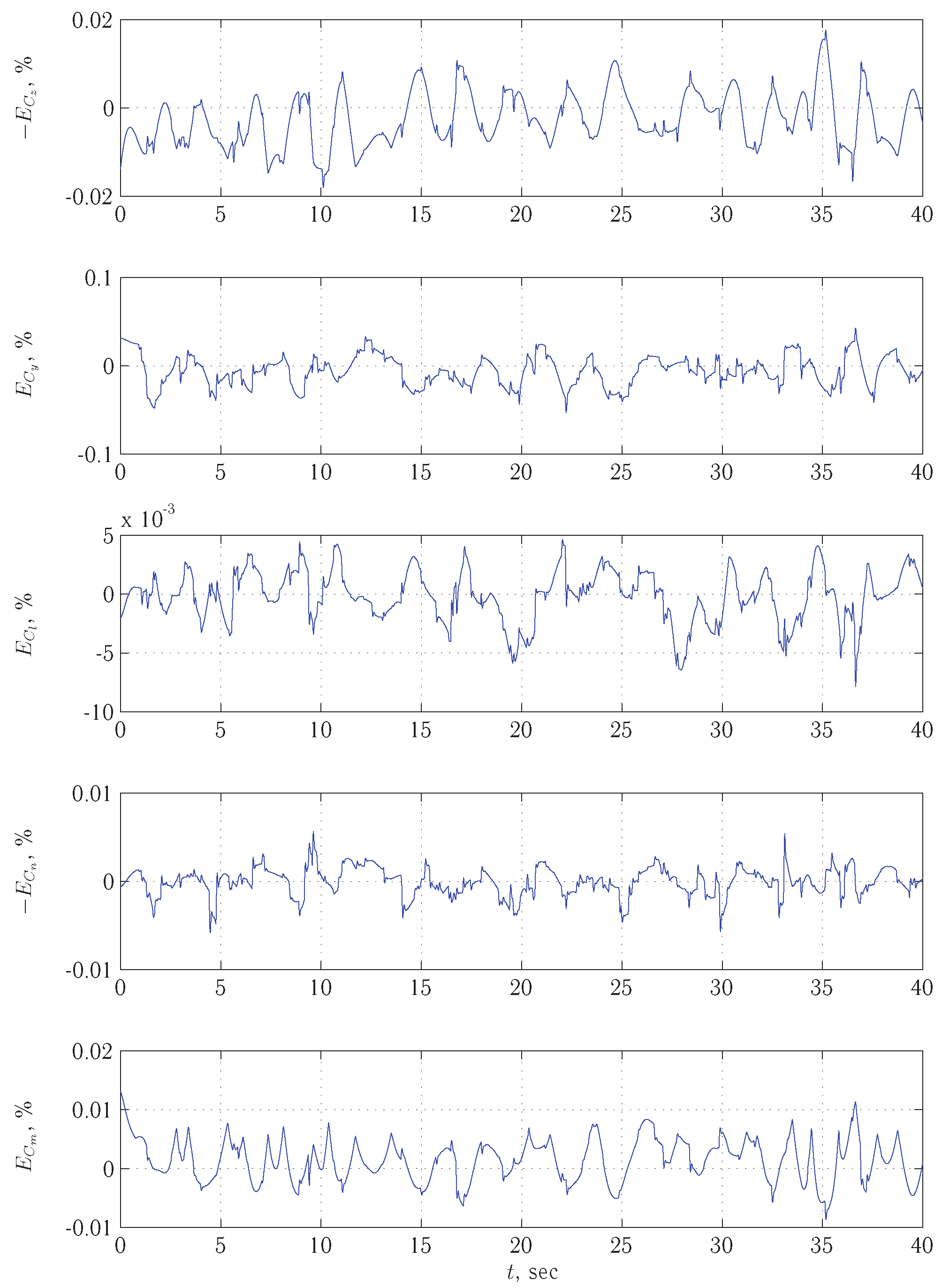This is an integral estimate of the accuracy for the mentioned dependencies. In addition, the dynamics of changes in the current values of the reproduction error for $C_Y$, $C_l$, $C_n$, and $C_m$ in the process of testing the model are also interesting. These data, shown in Figure 18, show that the error level changes insignificantly over time; no significant changes in it, which could adversely affect the adequacy of the empirical ANN model, are detected.

It has to be noted that the semi-empirical approach to solving problems of modeling and identification of controlled dynamical systems requires a rather large consumption of computational resources for its implementation. In comparison with it, traditional variants of solving such problems are much more economical. However, in our opinion, the higher computational resource-demanding nature of our approach pays off with the advantages it provides. Namely, as noted above, the main factors of uncertainty in models of aircraft motion are its aerodynamic characteristics, characterized by dimensionless coefficients of aerodynamic forces and moments. Each of these coefficients is a nonlinear function of several variables. The traditional approach to the problem of the identification of aerodynamic characteristics (see [39,40,41]) is based on linearization of these functions by means of their Taylor series expansion. This operation is performed “at a point”, i.e., for one particular combination of values of the arguments of the recovered function, rather than for the entire domain of their definition. The main advantage of the semi-empirical approach is that with its use we can reconstruct from experimental data the above-mentioned nonlinear functions of many variables as holistic objects in the whole range of changes in the values of their arguments with high accuracy. In other words, firstly, there is no need for linearization of these functions, and secondly, the obtained solution is no longer bound to a single specific combination of values of the function arguments.

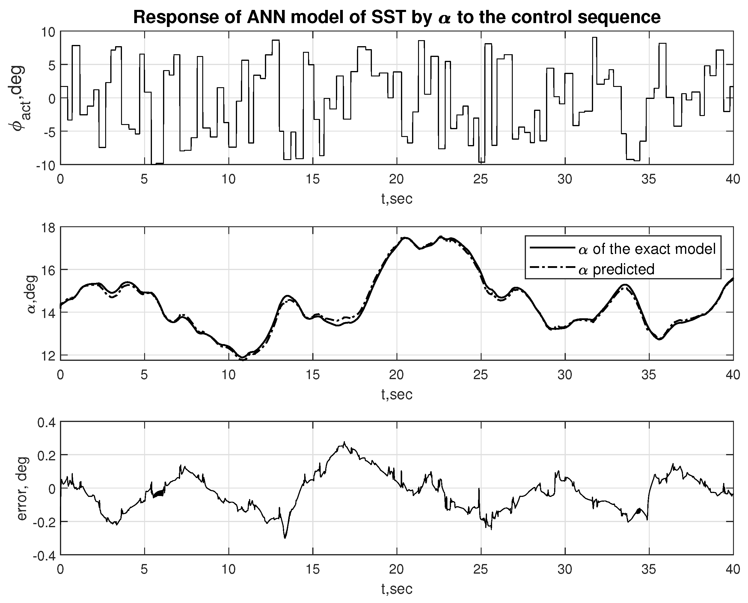
5. Deep Learning Techniques for Modeling and Controlling Aircraft Motion

So, the use of semi-empirical ANN models of aircraft motion allows us to overcome the complexity threshold that takes place for empirical ANN models. However, the price to be paid for this achievement will be unacceptably high in some cases. These are the situations when it is necessary to promptly correct the ANN model in order to restore its adequacy to the object with changed properties. For such applications, semi-empirical ANN models are absolutely unsuitable. They can be successfully applied, as was shown in the previous section, to those tasks where online adjustment of the model is not required. In particular, one of the most important problems of this kind is the identification of aerodynamic characteristics of aircraft with their representation in the form of nonlinear functions of many variables, with high accuracy in the whole area of definition of these functions.

However, as noted in the introduction, in addition to semi-empirical ANN models, there is another alternative approach to overcoming the complexity threshold inherent in recurrent ANN models of the black-box type. This approach produces models of the same category, i.e., they too will be of the black-box type. However, such models will nevertheless also be hybrid models by combining both feedforward and recurrent layers in the same model. This makes it possible to build motion models involving deep neural network technology and deep learning methods. In such a variant, it becomes possible to implement algorithms for online adjustment of models, i.e., they become potentially suitable for their use as part of adaptive control systems.

A considerable number of publications have been devoted to the present moment to the formation of controlled dynamic systems models based on deep learning methods, e.g., [138,139,140,141,142,143,144,145,146].

Let us demonstrate the capabilities of the combined approach based on deep learning methods by using the example of forming a model of a control object and using this model to realize adaptive fault-tolerant control for the problem of longitudinal angular motion (31). As a control object, we will consider, as in the example with the NARX model, a supersonic transport airplane (SST) [118,119].

5.1. Deep Neural Network as a Model of Aircraft Motion

The ANN model of SST motion being formed is a combination of convolutional layers and long short-term memory (LSTM) layers. A number of different connection structures were compared for such a network. The sequential configuration shown in Figure 19 was found to be the most rational.

The network used for modeling SST motion consists of an entry layer and four sets of layers that perform specialized functions.

The entry layer in the structures shown in Figure 19 is, as is usual in neural networks, a set of elements (memory cells) that contain the current value of the input vector components. For the structure in Figure 19 (the SST motion model), these are the five components from the motion model (31): four states (angle of attack, pitch angular velocity, deflection angle, and deflection rate for the elevator) and one control component (the command signal for the elevator actuator).

The first set starts with a one-dimensional convolution layer, which performs a convolution operation for input elements of size $5\times 1$. This allows the layer to select fragments of the input data and search for patterns among them. Such fragments are called convolution kernels. There are 16 neurons in the layer. The data processed by this layer goes to the layer that performs the ReLU operation. The ReLU layer is followed by a layer of one-dimensional subsampling (pooling) of the average pooling type, which averages one-dimensional data with a step of four units.

The second set of layers resembles the first, but with 32 neurons. The other two layers in the set perform the same operations as in the first set.

The third set of layers involves elements of neural network memory. For this purpose, we use a layer of the LSTM type applied in sequence-to-sequence tasks, i.e., the transformation of one sequence into another. In our case, the input action on the dynamical system influences the response of the dynamical system to this action as a function of time. This layer consists of 100 LSTM neurons.

Following the memory layer is the fully connected layer. Its purpose is to approximate the data stored in the LSTM memory layer. The fully connected layer contains 100 neurons.

In artificial intelligence systems using LSTM memory, there is usually a dropout layer. Such a layer removes some neurons by selecting them randomly. This technique allows for so-called regularization, which improves the convergence of the learning process. In this case, the dropout coefficient is chosen to be 0.1. This means that 10% of neurons are eliminated.

Finally, the output of this set is the activation sigmoid function, which introduces nonlinearity into the approximated surface and cuts off the results below a certain threshold.

The fourth set of layers is the output for the whole neural network. A fully connected layer of a single neuron compresses the data, which has already passed all layers of processing, into a one-dimensional array, which is then fed to the layer that performs nonlinear regression of the input data by the RMS error criterion.

The network of this architecture was successfully trained, requiring several thousand epochs. The training results are shown in Figure 20. The trained SST model predicts the angle of attack by responding to the generated random control. The current modeling error does not exceed 0.3 deg, which is quite a satisfactory result for the problem under consideration.

We have demonstrated in this example that using a hybrid model obtained by combining feedforward and recurrent neural networks, it is possible to simulate the behavior of even such complex dynamic objects as SST with acceptable accuracy. In this model, the feedforward network (a convolutional network based on one-dimensional convolution, Conv1d) preprocesses the signals received at the input of the LSTM layer, which reproduces the dynamics of the modeled object. Then follow again the feedforward layers, which postprocess the outputs of the LSTM network and form the value of the state variables of the control object for the next moment of time. The purpose of this example is to show that it is possible to successfully model complex dynamics by combining elements of feedforward networks and recurrent networks. Of course, this model is related to a specific object (SST in our case); when working with other objects, it will be necessary to form other combinations of the mentioned elements adequate to these objects.

5.2. Neural Network Adaptive Control of Aircraft Motion

There are a number of adaptive control schemes that use neural networks [116,147,148,149,150]. One of the most popular among them is the MRAC (Model Reference Adaptive Control) scheme [151]. A possible variant of its neural network realization is shown in Figure 21. This scheme is specialized to solve the tracking problem for a certain reference signal. The requirements for the desired properties of the system under the influence of the neurocontroller are expressed using a reference model.

As we can see from Figure 21, the system based on the MRAC scheme includes two neural networks as elements: for the object model (Figure 19) and for the controller (Figure 22). To adjust the controller using the error backpropagation method, we need to know the mismatch $\tilde{u}-u^{*}$ at the output of the neural network implementing it. This mismatch leads to inaccurate control of the object with error $y_{rm}-y_p$. We cannot, however, compute the value of $\tilde{u}-u^{*}$ since we do not know the “correct” value of $u^{*}$ but can only measure the error $y_{rm}-y_p$. Therefore, an ANN model of the control object is included in the MRAC scheme to allow us to use $y_{rm}-y_p$ instead of $y_{rm}-\widehat{y}$. Thus, we compare the output of the reference model $y_{rm}$ not with the output of the object $y_p$ but with the output of the ANN model $\widehat{y}$. This allows us to convert the error $y_{rm}-\widehat{y}$ into a mismatch $\tilde{u}-u^{*}$ using the standard error backpropagation method. However, with this approach, we train the neurocontroller to control not the object of interest but its ANN model. The inevitable inaccuracy of this model must be compensated for in some way. For this purpose, we consider that the error of the ANN model is nothing but another disturbance that must be considered when controlling our object. To compensate for this disturbance, a compensating PD feedback on the ANN modeling error is introduced into the MRAC structure, as shown in Figure 21.

The ANN model of the control object was created for use in the MRAC scheme, shown in Figure 21. As mentioned above, such a system includes a neurocontroller, the structure of which is shown in Figure 22. We have synthesized this neurocontroller using deep neural network technology, which is currently finding increasing application as a tool for solving control problems for various dynamical systems [152,153,154].

The neurocontroller under consideration consists of several layers. First comes the entry layer, which contains two components: the reference signal r (the reference signal for the angle of attack in the considered case) and the current value of the control object output (the current realized value of the angle of attack). The next layer, containing 200 neurons of the LSTM type, performs the function of memory. The following fully connected layer approximates the data transferred from the LSTM layer. The dropout layer removes 10% of the randomly selected neurons, thus improving the convergence of the learning process. The activation sigmoid function adds nonlinearity to the approximation process. Data below a certain threshold is cut off. Finally, the last fully connected layer of one neuron produces the result with the dimensionality expected by the pre-trained ANN model of SST.

Obtaining the source data for training the combined network, including the ANN controller and ANN model, is based on a procedure of random sequence generation similar to the one described above. In this case, however, a random reference signal was generated for the angle of attack in the range from $-2$ to 11 deg for a time of 4 to 8 s, and then the response of the reference model to this signal was computed. The time step was 0.01 s, and the total length of the sequence was 100 s. Then both the reference signal and the response to it were applied in training the neurocontroller. Moreover, similar to the training of the ANN model, several dozen sequences were generated for the neurocontroller, some of which were used only for its training and some of which were used only for testing. The source data for training the combined network and the results of training this network are shown in Figure 23, from which we can see that the trained neurocontroller controls the SST, producing control signals that allow tracking the target signal by the angle of attack with an acceptable error.

For the generated ANN controller, an experiment was conducted to test the created adaptive system for fault tolerance. A simulation of a failure that leads to a 50% decrease in the efficiency of the elevator rudder was performed. The behavior of the system after the failure, which occurred at 40 s, is shown in Figure 24. We can see that the tracking error value for the reference signal has increased significantly, which leads to the control system malfunctioning. Next, the pretraining of the coupled system (ANN model + ANN controller) was performed for 1600 epochs. The obtained results are shown in Figure 25. The operability of the control system under consideration was restored.

6. Conclusions

There is an important applied problem, which consists in controlling the behavior of a dynamic system under conditions of incomplete and inaccurate knowledge of the properties of the control object and the environment in which it operates. One of the most important classes of such systems is aircraft of various types and purposes. For them, the control task is further complicated by the fact that during flight various abnormal situations may occur, in particular, equipment failures and structural damage, which change the dynamic properties of the control object.

At the same time, for both control laws and control object models, it is not always possible to achieve success based on recurrent neural networks of the traditional kind (ANN models of the black-box type), which are quite often used for modeling dynamical systems and their control. In cases where the system has complicated dynamics, this approach is inefficient. As alternative approaches, we have considered two variants of hybrid ANN models that allow us to overcome the limitations inherent in traditional ANN models of controlled dynamical systems. The first of these options is based on the joint use of empirical data and theoretical knowledge about the control object. This option leads us to the gray box-type models (semi-empirical ANN models). The second option is based on combining elements of feedforward and recurrent networks. It makes it possible to use deep learning methods to develop the required ANN models.

The analysis of the capabilities and limitations of the considered approaches to solving problems of modeling and control for dynamical systems is carried out on examples related to supersonic passenger aircraft. The results of this analysis allow us to reveal the areas of preferable use for each of these approaches.

In addition to the mentioned variants, there are two more that are of considerable interest from the point of view of the control problem for a complex nonlinear dynamic object under uncertainty. These are the nonlinear dynamic inversion approach (NDI approach) and the approach based on reinforcement learning in a version of approximate (adaptive) dynamic programming (ADP approach). The joint use of these two approaches also seems promising. However, a review of the NDI approach and the ADP approach is beyond the scope of this paper. The authors intend to carry out such a review in the following publications.