A Conceptual Comparison of Hydraulic and Electric Actuation Systems for a Generic Fighter Aircraft

Abstract

This paper presents a methodology for evaluating different flight control actuation system architectures in the early conceptual design phase. In particular, this paper shows how hydraulic and electric actuators can be modeled even if very little is known about the aircraft design or requirements while still including the most dominant static and dynamic characteristics. Singular Value Decomposition is used to estimate model parameters and actuator characteristics from industrial data. This is a quick way to estimate what is needed with little input. The purpose of the models is to predict the power consumption, cooling needs, weight, and size. This is performed by integrating the actuator models in a dynamic simulation framework that also includes a flight simulator and surrounding systems. The results from subsystem studies support the aircraft design process, where actuator characteristics affect the engine performance and aircraft sizing. The methodology is applied to a generic fighter by comparing hydraulic and electric actuation system architectures. Besides providing a generic approach to the actuator modeling, the parameters that affect both the static and dynamic characteristics of an electromechanical and electrohydrostatic actuator are estimated with reasonably good accuracy with only four design parameters as input.

1. Introduction

The conceptual design phase in aircraft design is where the design space is explored, trade studies are made, and the requirements are balanced [1]. The main objective is to size the aircraft for its intended mission. Less focus is typically put on the on-board systems, and initial estimations on sizing typically rely on historical data. The challenge arises when new designs and technologies are considered, which was raised by [2,3]. It is stated in [4] that a third of the total empty weight comes from the aircraft systems, which further necessitates the need to include more detailed studies of the on-board systems early in the conceptual design phase.

This work presents a methodology for comparing different primary flight control actuation system architectures in the early conceptual design phase. Although any technology is applicable, a comparison of hydraulic and electromechanical actuators for a generic fighter has been made to illustrate the methodology. The results also give valuable insight into the challenges with electric actuation for this type of aircraft.

A well-balanced on-board system architecture must be created on the aircraft level where synergies between subsystems can also be considered. There are several proposals in the literature on methodologies and frameworks for evaluating system architectures at the aircraft level. The flight control actuation system has been a particular point of focus due to its impact on the entire architecture: its hydraulic or electric power supply, cooling solutions, weight, and size requirements. All have a large impact on the final aircraft size and power off-take requirements. A methodology linking the subsystem sizing with traditional aircraft sizing during the conceptual design phase is presented in [2]. The methodology is applied to a Boeing 787–800 by comparing hydraulic and electric flight control actuation. After sizing and evaluating the subsystem, characteristics such as the subsystem weight, non-propulsive power requirements, and drag coefficient change are fed back to the aircraft and propulsion system sizing

In [5,6,7], an integrated framework for modeling and comparing different aircraft system architectures with a focus on more electric aircrafts is presented. A Functional Mock-up Interface facilitates the co-simulation of different domains, and a case study was adopted for the flight control system of the Airbus A320. The models include mass and performance and can be realized at different levels of detail depending on the computational burden. Architectures are analyzed with respect to weight, non-propulsive power requirements, and fuel burn.

A modeling methodology based on ARCADIA/Capella is proposed by [8] that allows for the traceability, encapsulation, and visualization of system architectures at different levels of granularity and abstraction applied to the flight control system (FCS). This allows for both functional and logical representations of the FCS. A platform referred to as Virtual Iron Bird for assessing aircraft system configurations is presented in [9]. The Modelica language is used for an inverse modeling approach to analyze the behavior and power consumption. An inverse modeling approach is also used in [10] for subsystem sizing while the performance and power consumption are analyzed with direct models. The authors emphasize that new technologies require a more integrated design approach at a global level. The initial design and configuration of the aircraft and requirements are inputs to the on-board system simulation framework. The power requirements are calculated for the entire mission, together with the mass and drag, affecting the total fuel burn of the aircraft. A functional-driven design approach is used in [11] to enable a functional enhancement of the FCS through new technologies and moving toward MEA. A framework is developed in [3], where the FCS design is integrated into the conceptual design phase using advanced methods generating higher fidelity models. A flight mechanics model is developed that enables a detailed analysis of the stability and control of the FCS. The electric flight control system is optimized in terms of size, weight, and efficiency while meeting reliability requirements in [12]. A set of constraints is defined to narrow the design space, where hydraulic and electric actuators are included. A genetic algorithm is set up for the multi-objective optimization problem to find possible permutations. The framework in [13] integrates geometric, aerodynamic, and dynamic models for optimizing and evaluating on-board system architectures. The main idea is to increase confidence in a conceptual design by adding more information. Also here is inverse modeling supported. The power consumption is simulated over the flight mission and given as input to surrounding systems. The average is given as input to the cooling system, and the increased power need is added to the total. A framework for the multi-objective optimization of actuators is presented in [14] that uses parametric models to include the power chain, thermal characteristics, and structure. Surrogate models are used for the latter two.

It is clear from the literature that the complete aircraft system architecture needs to be analyzed at the aircraft level for characteristics including total fuel burn, weight, size, power extraction, and cooling needs. Supporting studies of the subsystems in detail are required. The earlier this can be conducted, the more confidence is put in the design. The question is how to represent the flight control system architecture at a more detailed level early in the conceptual design phase when very little is known about the subsystem requirements or the design. This paper proposes a design method that relies on Singular Value Decomposition and regression models to support the modeling of the most dominant actuator static and dynamic characteristics. Generic models of the actuators are developed that allow for a quick reconfiguration of the design characteristics. The actuator models are integrated into a framework for time-varying simulations that represent the whole aircraft that is used for both system sizing and analysis. A case study compares a servohydraulic, electromechanical, and electrohydrostatic flight control system architecture for a generic supersonic fighter.

2. Delimitations

Part of this work is based on company data. Due to confidentiality, the data cannot be made public. The methodology is fully described, but all results from the case study are presented in relative terms. The point is to highlight the difference between the studied architectures by applying the defined methodology. The scope is not to favor any technology. The presented case study is based on a fictive aircraft with fictive requirements. A different set of requirements might therefore give a different result. The authors do not put any value into the actual results other than showcasing the methodology. Where possible, the methodology was validated against open data. The methodology can be applied to other aircraft configurations but would require data at a subsystem level from a reference aircraft. However, the method of constructing actuator models based on open data can be expanded to other subsystems.

The methodology presented is to be viewed from an early aircraft conceptual design phase, supporting aircraft concept evaluations. It is assumed that very little knowledge about the subsystem requirements is known with few available data in this phase, and as such, the accuracy of the results reflects these preconditions.

3. Actuators’ State-of-the-Art and Model Requirements

The traditional flight control actuation system uses servhohydraulic actuators (SHAs) but is slowly evolving toward more electrified alternatives. On the latest development front, Airbus, Boeing, and Lockheed Martin stand with their respective uses of electrified actuators. Airbus’s A350 and A380 fly with electrohydraulic actuators (EHAs) and electrohydraulic backup actuators (EBHAs) on primary control surfaces [15], Lockheed Martin’s F35 is equipped with EHAs on all primary control surfaces [16], and Boeing’s 787 flies with electromechanical actuators (EMAs) on the spoilers [17].

The major actuation technologies are well-described in the literature [18]. A brief overview is given here for completion. Figure 1 illustrates the three major technologies available today. The SHA is driven by a servo valve supplied with hydraulic pressure from a centralized system, although local systems are being explored [19]. An integrated valve manifold provides the necessary safety functions. The EHA is an integrated unit with an electric motor, a hydraulic pump, a valve manifold, and a cylinder. Since it only consumes power when activated, it is classified as a power-by-wire actuator. The EMA is also a power-by-wire actuator consisting of an electric motor driving a ball screw, either directly or through a gearbox. Although a gearbox can reduce the EMA weight, it adds to the complexity, reflected inertia, and backlash. Other types of actuators are also available, such as the EBHA, or even rotary.

Although the servohydraulic actuator is the common solution, there are some general drivers for a technology change. Some of these should be regarded in the wake of the more electric aircraft philosophy.

• Overall, it is believed that electrifying the actuation system will lead to lower cost, lower weight, easier maintenance, and increased safety and availability, which is supported by [20,21,22]. The removal of the centralized hydraulic supply would be a great contributor.
• Electrical actuators are easier to maintain and install, especially the EMA. The EMA has a very good storage capability.
• Increased survivability since segregation and damage protection are higher for electrical actuators. However, hydraulic actuators are a mature technology and offer an easy way to accommodate failure modes. This is something that is inherited by EHAs but has been proven to be more difficult for EMAs.
• Thermal management is inherently made easy with hydraulic actuators due to the constant circulation of oil that also transports away heat. An electric actuator must either be designed to withstand the heat or it will require external cooling. Another consideration is the potential heating of the actuator in very cold conditions.
• The energy efficiency of hydraulic actuators is poor due to the constant pressure system, leakage, and throttle control. The more efficient electric actuators will have positive effects upstream. There are, however, modes of operation that are less beneficial for electric actuators. Load holding would require a constant current unless a break is used, and very dynamic movement requires energy to accelerate the electric motor.
• The usage of one common power source among the subsystems could enable sophisticated energy management strategies with potential benefits on a platform level. This is in contrast to a centralized hydraulic system where a power exchange with the electrical system would be cumbersome and inefficient.

Modeling and simulation of these actuators are performed in the literature to varying degrees of accuracy. Often, weight is the focus, where the dynamic and thermal properties of the actuator are left out of the analysis; see, for example, [2,23], in which actuator systems are compared at a platform level. In some aspects, this is justified. For example, ref. [24] showed that the dynamic properties of an actuator, such as its power consumption and cooling requirements, are insignificant compared to its weight and size, and that its impact on fuel consumption is negligible. However, what is often overlooked is that the dynamic properties of an actuator can have a significant impact on its weight and size [25] as well as on the performance requirements of other systems, such as electrical and hydraulic supply systems or cooling systems. For electric actuators, the dynamic aspects become even more important. An EHA and EMA must accelerate the inertia present in the motor’s (and pump’s) rotating parts. Rapid accelerations place high demands on the supply of electrical power, which furthermore gets dissipated locally in the actuator upon deceleration. Thermal solutions are rarely taken into account in the literature when estimating actuator weight and size. It is possible to recuperate energy back to the aircraft’s electrical system, thus reducing the local heating that would otherwise occur. However, the efficiency of energy recuperation is usually limited, which ultimately still leads to local heating of the actuator [18]. A major challenge in product development, and thereby model development, is knowing what effects to consider and what to neglect to successfully meet an engineering task. For this reason, [26] proposes a matrix view to be used to relate modeling needs with modeling effects.

4. Methodology for Comparing System Architectures

To put the work in this paper in context, an overview of the interaction between aircraft-level studies and subsystem-level studies is illustrated in Figure 2. At the aircraft level, traditional sizing takes place based on the intended mission to be performed. This also includes the balancing of requirements and definition of the on-board systems architecture. The focus of this paper is the studies that take place at the subsystem level to support the aircraft design by going into more detail about the subsystem architecture and components. The respective KPIs are evaluated at both levels, and a continuous and iterative exchange of knowledge in terms of models and data takes place. This means that design solutions and models are improved as more knowledge is gained about the system and the requirements. The exchange between the aircraft and subsystem levels indicates that any new knowledge gained should lead to an update at the opposite level.

A powerful tool to represent system knowledge is the use of ontologies representation that works at all system levels, as shown in [27,28,29]. An ontology was used in [28] to establish the interconnection and dependencies among related components and subsystems of the actuation system, leading up to different cost categories. This would include the power take-off, any bleed air consumption to cool the equipment, and the additional thrust requirements due to the increased parasitic (from the structure and possible ram air intakes) and induced drag. The induced drag results from the equipment’s weight and the structural penalty, as well as the additional fuel to carry the equipment. This information was used here to support the development of the analysis architecture, with a focus on the operational cost (typically fuel burn). The analysis architecture, see [30], describes what models are needed for the intended analysis and the relation between simulation models. The evaluation of the architectures requires different levels of model fidelity depending on the needs and purpose. A classification of different levels is performed in [31]: Level 0—statistical models based on existing aircrafts; Level 1—logical representation of physical elements and steady-state models; Level 2—static and dynamic modeling capturing the most important phenomenon; Level 3—highly detailed and accurate modeling (e.g., power electronic switching and FEM thermal models).

Adopting this definition, the actuation system study and architecture comparison implement representations at different fidelity levels as the design progresses. However, including studies at Level 2 early in the concept phase would give more confidence in the design choices. This can be performed by a more generic modeling of the actuation system including the most relevant dynamic characteristics and integrating these in a simulation environment that also includes the necessary interacting systems like a flight simulator and other vehicle systems, as illustrated in Figure 3. Different systems are selected and represented with different fidelity levels depending on the specific study. Considering the flight control actuation system, the integration of a 6-DOF flight simulator enables the estimation of a more realistic control surface behavior and a more proper control surface command allocation for different flight maneuvers and mission segments compared to a static assumption of the control characteristics. This not only allows us to better estimate the actuator dynamic response and power consumption, but it also gives an estimate of the total power consumption during the different mission segments.

The work flow in Figure 2 follows several steps where the simulation framework is used in an integrated manner to support the development work. The complete on-board system architecture is defined at the aircraft level, where balancing aircraft and subsystem requirements takes place together with sizing and mission evaluation. The subsystem requirements and initial assumptions become the starting point for subsystem-level studies; in this case, the flight control actuation system. The actuation system architecture is further defined based on the top-level requirements and an initial system safety analysis, defining the required redundancy levels for actuators and supply systems. Military aircraft requirements are based on the intended operational scenario. The simulation framework is therefore used to find dimensioning maneuvers and actuator requirements, which are used for actuator sizing. Properly sized actuator models are then integrated into the framework to support the supply system sizing. This work is eventually iterative as the design evolves.

The model of the actuator is represented in Figure 4. The purpose of the model is to evaluate the actuator’s weight, size, power consumption, and cooling needs for a set of requirements. The requirements describe the maximum force (intermittent or continuous), maximum speed (e.g., at no load), maximum power, and stroke. The power in this case helps to better define the electric motor characteristics since it also depends on the operating envelope and not only on maximum torque and speed. Including dynamic properties improves the power consumption estimation, which might have a great impact on the power supply sizing. How this can be conducted is exemplified in Section 5. Contributions to parasitic drag are excluded here. The reason is that it requires a more detailed design and knowledge, which is assumed to not be the case for this paper. It would involve a CAD representation for packaging, possible integration of actuator fairings, and CFD analysis. Early estimations in previous work have also shown its contribution to fuel consumption to be much lower than system weight. However, an initial estimation of the required actuator space can be interesting during the early conceptualization to give an idea of the space and packaging requirements. For the completion of the analysis architecture, the supply systems are also included. Since it is not the particular focus, a steady-state representation is sufficient to support the actuation system analysis, including weight and size. Furthermore, an atmosphere model serves both the actuation system to provide the ambient temperature for the cooling requirements estimation and the flight simulator. The flight simulator includes the 6-DOF flight mechanics, a first CFD aerodata model, flight control laws for aircraft stabilization and maneuverability, and an engine model to provide thrust (and specific fuel consumption if required by the study).

The characteristics of the actuator, such as the weight, size, and necessary parameters for the execution of the simulation model, are estimated using Singular Value Decomposition (SVD). The strength of the SVD is that it can estimate the required characteristics based on only a few inputs. The initial work is presented in papers [32,33]. Due to the lack of aerospace data, the approach is to rely on industrial data that are openly available. The weight and size of the constituting components can be estimated and the total weight and size calculated from the sum of its parts. The same goes for all required model parameters. An actuator designed to specification will of course be optimized to fulfill the requirements and the estimated characteristics of a corresponding actuator will differ. The model can be tuned to fit a sample flight actuator if available.

5. Case Study

A case study that uses the proposed framework for comparing fly-by-wire servohydraulic, electromechanical, and electrohydrostatic actuation architectures for primary flight control actuation is presented here. The purpose is primarily to showcase the methodology that provides the weight and size distribution, power consumption, and cooling needs by integrating models in a full flight simulator environment containing more details than what is typically the case in the early aircraft conceptual design phase. This involves the definition of the architectures, development of proper models, and integration into the framework. The system boundary is defined from the engine power take-out shaft to the flight control surfaces.

The aircraft under consideration is fictive, and as such, the requirements are also fictive. Nevertheless, a realistic approach was taken when developing the architectures. The methodology and framework can therefore be adopted to similar studies where data are available. The results also give a sense of the difference between the technologies under consideration.

Since the modeling process is partially based on company data, no numbers can be disclosed and a relative comparison is provided. It is possible to conduct a similar study with any available data by following the same procedure.

5.1. Aircraft Configuration

The starting point is an already-defined aircraft configuration, see [34]. A general delta canard fighter is available for research purposes and is used as a baseline. The aircraft configuration parameters are found in

Table 1. Aircraft configuration parameters from [34].

Parameter	Value	Unit
Wing area	45	m2
Wing span	10	m
Wing chord (mean)	5.2	m
Mass	9100	kg
Ix	21,000	kgm2
Iy	81,000	kgm2
Iz	101,000	kgm2
Ixz	2500	kgm2

. There are seven primary control surfaces: two canards, inner and outer elevons for each side, and one rudder.

5.2. Actuation System Architecture Definition

For the comparison to be valid, the three architectures are designed to meet the same system requirements. The architectures are designed to meet the requirement of no single-point failure leading to a catastrophic event. A catastrophic event is here considered a loss of control surface actuation. Although safety functional requirements could have an impact on the actuator characteristics, for example, mechanical disconnect devices or dampers in the case of EMAs, and the loss of single control surfaces could be handled by a reconfiguration of the control surface allocation, such definitions would require a more detailed analysis provided in later design stages. The architectures need to consider the loss of the actuator, loss of the power supply, and loss of the engine. Some assumptions are made: a tandem cylinder is typically adopted in military applications, where the risk of cylinder jamming is acceptably low or mitigated, and it is assumed that the EMA ball screw is equally treated. This assumption should in practice be supported by supplier data and safety analyses, but it is a good starting point for this study where such data are not available.

Each control surface shall have a no-load rate of at least 50°/s. The required stall loads are derived from a simulation, as described in Section 5.5. The design of the architecture shall be considered to be safe against single points of failure.

The hydraulic architecture is the baseline for the comparison and is a traditional fly-by-wire architecture. The main gearbox, which is cooled by recirculating oil, drives two main hydraulic pumps. The hydraulic systems are separated. The pumps provide the necessary hydraulic oil at 28 MPa. Each system is cooled by circulating the oil through a heat exchanger. Each primary actuator is of a duplex configuration mechanically attached with a lever to the control surface. The two separated hydraulic systems with duplex actuators ensure full control if one system fails. If the main gearbox is lost but the engine is still running, bleed air can drive the auxiliary gearbox and pump to provide pressure to system 1. If the engine flames out, a small electrohydraulic pump driven from a 28 VDC battery provides hydraulic pressure for 10 min to maintain control while restarting the engine or to perform a controlled emergency landing. The architecture is shown in Figure 5.

The fully electric architecture, depicted in Figure 6, is valid for both the electromechanical and electrohydrostatic solutions. It has the same basic layout as the hydraulic one but utilizes state-of-the-art electric power and distribution. The main gearbox drives two wild frequency generators. The AC power is rectified and controlled to 270 VDC. A distribution unit based on solid-state technology provides the power to each actuator. The two main systems are separated. The gearbox, generators, rectifiers, and controller units are cooled by oil.

For the EMA case, the actuators are direct driven dual redundant electromechanical actuators with one common mechanical ball screw and a dual redundant permanent magnet motor. It is assumed to be sufficient to handle the safety requirements for this study.

The EHA is assumed to be of duplex type with a tandem cylinder, two pumps and motors, and a small accumulator to provide sufficient oil.

Each actuator requires its own duplex Remote Control Unit (REU) for motor speed and position control. This unit converts the constant DC voltage to an alternating motor voltage for each of the motor’s phases. The actuators could be cooled by liquid, forced air, or natural convection, depending on the needs. However, due to the weight penalty of a cooling circuit, it is assumed that the actuators do not require any active cooling. This assumption is to be verified by the analysis. A bleed-air-driven gearbox and generator provide power in case of the loss of the main gearbox, similar to the hydraulic architecture. A 270 VDC battery provides power for 10 min in the case of the loss of the engine.

5.3. Flight Simulator Environment

The simulation framework utilizes the Admire flight simulator. It is an open model developed by the Swedish Defense Research Agency for research purposes and is well described in [34]. It provides a six-degree-of-freedom flight mechanical model, an engine model that provides thrust, an atmospheric model, an aero data model with all necessary aerodynamic forces and moments, a sensor model, and flight control laws that stabilize and handle longitudinal and lateral control.

5.4. System Modeling

The system modeling is focused on modeling the actuation and vehicle systems, considering weight, size, power consumption, and cooling needs. The executable models are implemented in Matlab/Simulink (version 2022b) using the Simscape library.

• Servohydraulic actuator
• Weight and size

The weight and size estimation of the SHA is based on not publicly available aircraft data. Three different-sized duplex/tandem hydraulic primary actuators from an existing aircraft are used as input. A standard linear regression is applied and a relation was found between the actuator weight, M, and size, V, to stall force, F, and stroke, l, according to Equations (1) and (2). The coefficients $k_1$ and $k_2$ (M and V for mass and volume) are found from the linear regression:

$$\begin{array}{cc}\hfill & M_{SHA}=k_{M1}F+k_{M2}l\hfill \end{array}$$

(1)

$$\begin{array}{cc}\hfill & V_{SHA}=k_{V1}F+k_{V2}l\hfill \end{array}$$

(2)

• Simulation model

The executable SHA model is defined in Figure 7. It includes the nonlinear steady-state characteristic and the dynamic characteristic deemed necessary; that is, the integration from actuator movement. The important characteristic is the actuator position since it affects the flight dynamics and the actuator speed since it affects the power consumption and thermal properties. Any internal states, such as servo valve dynamics and pressure build-up, are excluded since they only concern the high-frequency spectrum and require more detailed design and modeling. The advantage of implementing the model as a closed-loop system is that both position and speed are calculated without any derivation.

The closed-loop response is defined by the proportional gain $K_p$, the hydraulic gain $K_q$, and cylinder size $A_p$. The valve opening A is defined from the control signal as in Equation (3):

$$A=K_p(x_{cmd}-x)$$

(3)

where x is the actuator position. A saturation block limits the maximum allowed speed. The limit $A_{max}$ can be defined according to Equation (4):

$$A_{max}={\displaystyle \frac{q_{max}}{C_q\sqrt{\frac{1}{\rho }{p}_s-p_{l,nom}}}}$$

(4)

The maximum allowed flow $q_{max}$ is based on the defined maximum speed $v_{max}$, while the nominal load pressure $p_{l,nom}$ is based on the nominal load according to Equations (5) and (6):

$$\begin{array}{cc}\hfill & q_{max}=v_{max}·A_p\hfill \end{array}$$

(5)

$$\begin{array}{cc}\hfill & p_{l,nom}={\displaystyle \frac{F_{nom}}{A_p}}\hfill \end{array}$$

(6)

The maximum speed is either defined at the no-load case, where the nominal load is set to zero, or at a continuous load value. The tank pressure, if any, could also be included but is neglected here for simplicity reasons. The hydraulic gain $K_q$ defines the nonlinear steady-state characteristic based on the flow coefficient $C_q$, oil density $\rho$, and pressure difference over the servo valve as in Equation (7):

$$K_q=C_q\sqrt{{\displaystyle \frac{1}{\rho }}(p_s-p_l)}$$

(7)

with supply pressure $p_s$ and load pressure $p_l$. Both $C_q$ and $\rho$ are user-defined and are here set to typical values of 0.7 and 850, respectively.

The block diagram in Figure 7 can be turned into a first-order transfer function on the general form in Equation (8), where s is the Laplace operator and $\tau$ the first-order response time:

$$G_{gen}={\displaystyle \frac{1}{\tau ·s+1}}$$

(8)

The response varies with the load since the hydraulic system is nonlinear. The response is typically defined for the no-load case. The open loop gain is defined from the block diagram as in Equation (9):

$$G_o={\displaystyle \frac{K_p{K}_q}{A_{p}s}}$$

(9)

The closed-loop response can now be defined as in Equation (10):

$$G_c={\displaystyle \frac{1}{\frac{A_{p}s}{K_p{K}_q}+1}}$$

(10)

The closed-loop response is compared with the general form, which gives the controller gain as in Equation (11):

$$K_p={\displaystyle \frac{A_p}{\tau K_q}}$$

(11)

A leakage term is added to account for the internal leakage of the system. A general model is adopted since no detailed data are available. The leakage is modeled using a variable orifice for each spool land of the servo valve (P for supply port, A and B for cylinder ports, and T for tank port): P-A, A-T, P-B, and B-T. The leakage is modeled according to the characteristics in Figure 8, where the maximum leakage occurs when the spool is centered and gradually decreases as the spool closes the corresponding land. The leakage is kept constant when the spool land is fully opened, illustrated by the negative side in the figure, and will be part of the main flow. The total leakage flow can be set to a typical value; around 1 L/min is used here.

• Electromechanical actuator

• Estimation of EMA characteristics

The estimation of the EMA’s characteristics is based on an SVD analysis. The EMA was reduced to include only the permanent magnet motor and ball screw since only a direct driven EMA is considered here. A more detailed modeling is possible using the same approach by including bearings and sensors as well, or a gearbox if such an actuator is considered. The process is illustrated in Figure 9.

An SVD analysis is produced for both the ball screw and the permanent magnet motor. The ball screw model takes the required force, speed, and stroke as input, where the stroke is needed to estimate the ball screw weight. The SVD models can be used in different ways. Model parameters can be estimated directly or design rules can be defined that sets the relation between the inputs and ball screw characteristics. This can be seen in detail in [32]. The pitch of the ball screw is estimated with the required actuator stall force as input, and it is used to transform the required force and linear speed to a motor torque and motor rotational speed.

An SVD model of the motor is produced, which estimates the size and weight, as well as all necessary parameters for the simulation model. The inputs to this model are the maximum torque, which is here derived from the actuator stall load through the ball screw; the maximum rotational speed derived from the actuator maximum speed; and the maximum power. The power is included since it gave a better estimation of the motor characteristics and can be motivated by the fact that motors with a similar torque and speed can have different power characteristics depending on certain design choices. The maximum power is here assumed to occur at 70% of the maximum torque–speed product. Of course, these are only assumptions, and without any detailed knowledge of the required torque–speed characteristics of the actuator, they serve as a good starting point. Based on these inputs, the model estimates the following parameters used for the weight and size estimation, as well as the simulation model: max allowed continuous current, torque constant, winding resistance, rotor inertia, thermal time constant, mass, and volume. The model is based on data from 64 different permanent magnet motors collected from [35]. Seven motors were excluded from the dataset to serve as validation data. These motors are designed for typical industrial applications and require a 400 V supply, which is different from the 270 VDC assumed for this paper. However, the model is also tested for an available flight EMA designed for 270 VDC. The total weight and size of the actuator is the sum of the ball screw and motor. The specific tool for deriving the SVD model is implemented in Excel, and the approach can be studied more in detail in [36].

An example of the validation of the SVD model is shown in Figure 10. The model finds the statistical relation between all parameters in the left-side column. By applying an in-built optimization routine, the motor parameters are estimated by tuning the SVD variables in order to minimize the defined criteria, in this case, to minimize the motor weight. Only three SVD variables are included since it turns out that three inputs have the most dominant effect on the design. The relative error between each estimated parameter and the actual value from the validation set is calculated. There is a large spread in how accurately the different parameters are estimated for the validation set. The mass is at worst at 15% error, with a median at 7%. The volume is at 37%, but only for one sample, with a median error at 17%. The torque constant has a median error of 6% and a continuous current of 15%. The most difficult parameters to estimate are the winding resistance, rotor inertia, and the thermal time constant, with the respective median errors at 27%, 68%, and 36%. The only parameter with a very large spread in the estimated values is the rotor inertia. This is an indication that more input data are needed to have a better estimation; for example, a better knowledge of the operating envelope. The assumption is, however, that this information is not available in this phase of the conceptual design, and the model overall presents a valid approach to estimate the motor characteristics from only three input parameters. In all cases, the maximum speed is estimated higher. This is expected since the required value is low due to a direct drive EMA being investigated and electric motors typically working in a high speed range. This also affects the maximum power that is also estimated higher. This is not a problem, though, since the required speed and power are fulfilled.

A test sample is available from a current flight EMA. To have a better comparison, the maximum speed and power are scaled to a 400 V motor. The estimated total EMA weight differs only by 4%, the torque constant differs by 40%, the winding resistance by 46%, and the rotor inertia by 17%.

The actuator control unit’s weight and size are defined to scale linearly with stall load based on an available reference unit. This can differ depending on the control unit’s architecture, functionality, and whether it is integrated with the actuator or stand-alone equipment.

• Simulation model

The executable EMA model is shown in Figure 11. The model fidelity is balanced in such a way to include what is deemed necessary dynamic characteristic at a Level 2 model fidelity. Since a detailed design of the actuator is not available at the conceptual design stage, the modeling must also consider what data are available at this point. A typical electric motor model involves the electromagnetic and inertial effects. The electromagnetic effects are of very high frequency and are excluded. Furthermore, the model is implemented as a direct current (DC) equivalent since the alternating current components are not of interest. Thus, the model includes the speed and position control loops. The thermal characteristics account for the copper losses, and the whole motor is considered a homogeneous mass.

An initial rate limiter prevents the flight control system from commanding a too-high speed. The commanded actuator position is converted to motor angle through the ball screw lead. Since the model assumes the motor current control loop to be infinitely fast, only the static characteristic is included. The motor torque is assumed to be proportional to the motor current as in Equation (12):

$$T_m=K_t·i$$

(12)

Both the motor torque $T_m$ and the external load $T_L$ act on the motor inertia J together with friction. The external load is converted from the translational load through the ball screw as in Equation (13), where L is the ball screw lead:

$$T_m=T_L{\displaystyle \frac{L}{2\pi }}$$

(13)

The ball screw friction depends both on speed and temperature, which can be seen in [37,38], and can increase up to six times at very cold temperatures [39]. The ball screw efficiency can reach up to 95% in low-speed conditions, ref. [40], which is applied in this work. The viscous friction coefficient can be calculated based on assumptions of maximum efficiency and operating points, as shown in Equation (14), where $F_{nom}$ and ${\omega }_{nom}$ are the nominal load and speed where the maximum efficiency $\eta$ occurs. To include the temperature dependency, the coefficient is scaled with the factor $k_{temp}$, which varies exponentially with temperature, being one at around 20 °C, as shown in [39]. Finally, saturation limits the maximum allowed motor current:

$$B={\displaystyle \frac{F_{nom}}{v_{nom}}}\left({\displaystyle \frac{1}{\eta }}-1\right)k_{temp}$$

(14)

The speed and position controllers are designed to give a first-order closed-loop system, and the respective controllers are identified using the same method as for the servhohydraulic actuator. The speed controller can be identified as in Equation (15):

$$G_{\omega }={\displaystyle \frac{J·s+B}{{\tau }_{\omega }·K_t·s}}$$

(15)

The time constant ${\tau }_{\omega }$ is the desired speed control closed-loop response. The controller takes the form of a PI controller. The time response should be defined to be much faster than the position control loop, typically at least ten times faster. In this way, the speed control response can be neglected when designing the position control loop. The position control open loop now reduces to a pure integrator, and the position controller is defined as a proportional controller as in Equation (16):

$$G_p={\displaystyle \frac{1}{{\tau }_p}}$$

(16)

The constant ${\tau }_p$ is the desired position closed-loop response. The output from the position controller is the speed control reference. Saturation prevents the controller from demanding a too-high motor speed.

The motor current is given directly from the motor model. The motor voltage U is calculated from Equation (17):

$$U=R·i+K_e·\omega$$

(17)

The motor coils’ resistance is denoted R, and the back emf constant $K_e$ is assumed to be the same as the motor torque constant. The input current from the DC power supply is calculated by assuming a constant efficiency for the converter (REU) and applying a constant power conversion as in Equation (18):

$$i_{in}={\displaystyle \frac{U_{motor}·i_{motor}}{U_{DCnet}·\eta }}$$

(18)

The temperature characteristic is based on the assumption of a homogeneous thermal mass and that the dominating losses come from the copper resistance. The thermal behavior is defined by Equations (19) and (20):

$$\begin{array}{cc}\hfill & Q_{loss}-Q=m_{th}·c·\dot{T}\hfill \end{array}$$

(19)

$$\begin{array}{cc}\hfill & Q={\displaystyle \frac{T-T_{amb}}{R_{th}}}\hfill \end{array}$$

(20)

The thermal mass is denoted $m_{th}$, c is the specific heat, T the equivalent motor temperature, $Q_{loss}$ the motor losses, $T_{amb}$ the ambient temperature, and $R_{th}$ the thermal resistance. The temperature transfer function can now be defined as in Equation (21), with the thermal time constant ${\tau }_{th}$ defined in Equation (22). The copper losses are simply calculated from the squared motor current multiplied by the copper resistance:

$$\begin{array}{cc}\hfill & T={\displaystyle \frac{Q_{loss}·R_{th}+T_{amb}}{{\tau }_{th}·s+1}}\hfill \end{array}$$

(21)

$$\begin{array}{cc}\hfill & {\tau }_{th}=R_{th}·m_{th}·c\hfill \end{array}$$

(22)

The ambient temperature can either be set externally to a fixed value, or in this case, it is calculated as the bay temperature where the actuator is located. A detailed design is required to obtain a good estimate of the bay temperature, but a first approximation is to assume that the bay temperature follows the skin temperature with a 10 min delay. The bay temperature is calculated from Equation (23), where M is the Mach number, and the atmosphere temperature, $T_{atm}$, is calculated from Equation (24), where h is the flight altitude. The first-order filter represents the time delay, where s denotes the Laplace operator:

$$\begin{array}{cc}\hfill & T_{bay}=T_{atm}(1+M^2·0.18){\displaystyle \frac{1}{10s+1}}\hfill \end{array}$$

(23)

$$\begin{array}{cc}\hfill & T_{atm}=288.16-h·0.0065\hfill \end{array}$$

(24)

• Electrohydrostatic actuator

• Estimation of EHA characteristics

The estimation of the EHA weight and size follows the same process as for the SHA and EMA, shown in Figure 12. The required force, speed, and stroke size the required cylinder. This is the same cylinder model used for the SHA. The cylinder is sized for a stall load at a maximum pressure of 28 MPa and converts the required speed into a flow $q_p$ that the pumps must provide. The EHA pump typically runs at a very high speed. By assuming a speed n, in this case, 10,000 rpm, the pump displacement $D_p$ is given by Equation (25).

$$D_p={\displaystyle \frac{q_p}{n}}$$

(25)

The pump-sizing model is based on open data of bent-axis pumps. The same principle can be used for any type of pump with available data. Collecting data from [41] on different pump sizes and their respective mass, size, and inertia and applying regression models gives the relations in Equations (26), (27) and (28) between pump displacement (with unit m³/rev) and pump characteristics (mass in kg, inertia in kgm², and size in m³). The pump inertia is added to the motor inertia:

$$\begin{array}{cc}\hfill & m=0.28·D_P+4.4\hfill \end{array}$$

(26)

$$\begin{array}{cc}\hfill & J=2·{10}^{-5}·D_p^{1.34}\hfill \end{array}$$

(27)

$$\begin{array}{cc}\hfill & V_p=7·{10}^{-5}+0.0016\hfill \end{array}$$

(28)

The pumps convert the cylinder pressure into a required motor torque through Equation (29). A pump efficiency of 80% is applied. This of course varies over the working envelope but requires more detailed modeling of the pump losses. The chosen efficiency covers the interesting working region and is representative for sizing, even if higher efficiencies can be achieved in practice. The sizing of the motor then follows the same principle as for the EMA case by applying the SVD motor model:

$$T_m={\displaystyle \frac{D_P\Delta p}{{\eta }_p}}$$

(29)

The EHA also includes an accumulator to cover for possible oil leakage and volume change due to temperature. It is assumed that the accumulator size is equal to the cylinder oil volume. In a similar fashion to the pump, the weight and size of the accumulator can be estimated based on regression models from available data. Collecting data from [42] gives the relation for mass and size based on the required accumulator volume $V_{acc}$ (unit liter) as in Equations (30) and (31):

$$\begin{array}{cc}\hfill & m=2.85·V_{acc}+3\hfill \end{array}$$

(30)

$$\begin{array}{cc}\hfill & V_s=1.8·V_{acc}+1.5\hfill \end{array}$$

(31)

The control unit follows the same model as for the EMA. The total mass and size is the sum of all components, number of pumps, number of motors, cylinder, accumulator, and controller.

Validation of the model can be performed by comparing it to the open data of existing electrohydrostatic actuators. Data of a dual tandem EHA tested on the F16 fighter aircraft is available in [18], with a stall load of 15.5 kN. By applying the size estimation method, the total (actuator + control unit) weight is only 5% lower than the actual actuator.

• Simulation model

Since the EMA and EHA are similar in terms of dominating dynamic characteristics, the same implementation can be used for the simulation model, as shown in Figure 11. Although the pump contributes to the total inertia the motor has to overcome, the pump displacement and cylinder is considered as a ratio between the load and motor defined by the ratio in Equation (32):

$$ratio={\displaystyle \frac{D_p}{A_p·2\pi }}$$

(32)

A viscous friction is applied for the motor with a nominal efficiency of 95%. The same model as for the EMA is used but without the temperature dependency. The pump is assumed to have a constant efficiency of 80%. The pump efficiency varies in reality with operating conditions and temperature but requires a far more detailed model than what is intended for this study. The assumed efficiency is conservative and sufficient for sizing purposes.

• Vehicle systems

• Weight and size

There are two approaches to estimate the weight and size of the supply and distribution systems. It is possible to follow the method used to estimate the EMA weight and size by collecting data and applying a linear regression or an SVD analysis. The challenge is to find appropriate data and detailed information on how components are interfaced. The other approach is to study an existing aircraft installation, which is available to the authors. The benefit is that actual installation effects and component interfaces are more easily covered, which improves the final estimation. The drawback is that just one sample was used in this study.

Since the weight and size estimation are based on company data, it cannot be revealed to the public. The models are divided into supply, distribution, and loads (power consumers), considering only the main components from the reference aircraft. The weight and size of the components are then scaled according to the reference aircraft.

• Hydraulic supply system:

The hydraulic supply system includes the main pumps, reservoirs, accumulators, connecting elements (related to the supply units), and the hydraulic oil cooler. Since the hydraulic supply pressure is assumed to be equal to the reference system, the weight and size scale proportionally to the required maximum oil flow. The oil cooler’s mass and volume scale with the total hydraulic system’s power losses.

• Main gearbox:

The same gearbox model is used for both architectures. Its mass and volume scale linearly with the required maximum total power. It includes an oil cooler which scales linearly with the gearbox losses.

• Hydraulic distribution system:

The hydraulic distribution includes the main manifolds and the hydraulic piping, including the hydraulic oil. The manifold scales linearly with the total maximum flow since a higher flow would require larger passages to avoid too-high pressure losses.

It is not straightforward to estimate the required piping length and size, and hence its mass, without a detailed design. There are many variables to consider. The approach is to compare with the reference aircraft and isolate the piping to the primary actuation system and scale it with the wing span, aircraft length, and total oil flow. The argument is that the piping extends across the aircraft and the wings, while a higher flow would require larger pipes to avoid a too-high pressure drop. The pipe’s mass is thus calculated as in Equation (33), where q is the oil flow, S the wing span, L the aircraft length, and the constants $K_1$ and $K_2$ are derived from the scaling:

$$m_{pipe}=K_{1,pipe}·q·S+K_{2,pipe}·q·L$$

(33)

The required pipe length follows the same approach but only scales with the wing span and aircraft length. The mass of the hydraulic oil follows the same principle as for the pipe mass.

• Hydraulic auxiliary and emergency systems:

The auxiliary pump is connected to one of the main hydraulic systems and shares the same reservoir. It is driven by the auxiliary gearbox, which in turn is driven by bleed air from the engine. The scale model therefore only considers the pump itself. The mass and volume scale linearly with the required oil flow. Since the auxiliary pump activates during a failure of the main system, only half of the total flow is required. The auxiliary gearbox is considered a complete package with an oil cooler and an air turbine to drive it. The mass and volume scale linearly with maximum power. The total mass and volume of the auxiliary system is the sum of these components.

The emergency hydraulic system consists of a pump driven by an integrated electric motor and connecting pipes. A 24 VDC battery supplies the motor. The system shares the same reservoir as the main system and is therefore excluded from the scale model. The pump and motor package mass and volume scale linearly with the maximum required oil flow in emergency mode. The battery’s mass and volume, on the other hand, scale with the required energy to drive the pump for 10 min. This time range was set arbitrarily for this case study. The battery weight and size are based on a single lithium-ion cell, for which data are available, for example, here [43]. The required energy is used to calculated the amount of required cells. An actual battery pack weighs more than the total number of cells. There is the battery management system, the battery case, and installation equipment. Since no feasible data are available for the two battery packs in this work, comparing on the cell level at least gives a rough estimate of the relative weight difference for the two architectures.

• Electric power supply system:

The electric supply system consists of the electric generator, rectifier, and control unit. The total weight and size scale linearly with the power. The equipment shares a common oil cooler whose size and weight scale linearly with the internal power losses.

• Electric power distribution system:

The electric power distribution system consists of solid-state power distribution units (the exact number is not considered here) and the electric wiring. The mass and volume of the distribution unit scale with the total power.

The estimation of the wiring mass is based on a reference cable from the reference aircraft, which is compared to pure copper of the same size. This gives a correction factor for the required insulation. The sizing of the wire follows the standard AWG tables, found for example here [44], for the required maximum current. The wire mass estimates according to Equation (34), where l is the wire length, A is the wire area (AWG size), $\rho$ is the copper density, and k is the correction factor:

$$m_{wire}=l_{wire}·A_{wire}·{\rho }_{cu}·k_{wire}$$

(34)

The required wire length is set to be the same as the hydraulic pipe length. This is of course an assumption, but it ensures that the electric and hydraulic systems are compared on equal terms. The wire size is based on the assumption that the power distribution units are placed close to the actuators to avoid unnecessary cable routing. The assumption is that 20% of the total length is sized for the maximum power draw and the rest is sized for the mean power draw for one actuator.

• Electric auxiliary and emergency systems:

The electric auxiliary system components are equal to what is already defined for the main system and run from a similar auxiliary gearbox as the hydraulic system. The electric emergency system relies on a 270 VDC battery. The mass and size scale linearly with the required energy content for 10 min of flight.

• Simulation model

The simulation models of the vehicle systems are at a high fidelity steady-state level and include a gearbox, hydraulic pumps, and generator. The models are implemented to calculate the input power required to drive the actuation system by assuming constant efficiencies, as shown in Equation (35). The energy efficiency is set to 90% for the gearbox and electric supply system (total efficiency) and 80% for the pumps:

$$P_{IN}={\displaystyle \frac{P_{OUT}}{\eta }}$$

(35)

5.5. System Sizing

Below follows the procedure for sizing all the involved systems. The above-defined framework and models are used to derive the requirements. The procedure is merely for illustrative purposes of the methodology and comparison of the two architectures. It is, however, chosen in order to have a realistic comparison.

• Actuator Stall Force and Speed Requirement

The flight control actuators are sized by simulating the 6-DOF model in various envelope points performing doublet maneuvers; that is, performing a roll while pulling the pitch and then immediately rolling in the opposite direction. This is motivated by the operational requirements of such an aircraft. The highest loads occur at low altitudes at high subsonic speeds. This, in combination with past experience, results in actuator stall load requirements: 115 kN for the outer elevons, 85 kN for the inner elevons, 85 kN for canards, and 50 kN for the rudder. The maximum control surface deflection is set to 50°/s at no load with a response time of 50 ms, as is defined by the flight simulator in use.

• Hydraulic System

The sizing of the SHA is straightforward by sizing the effective piston area according to the stall loads and assuming a supply pressure of 280 bars and a tank pressure of 6.5 bars. The maximum valve opening is calculated according to the model defined in Section 5.4 based on the no-load speed requirements, the hydraulic gain is calculated with the defined supply and tank pressure at no-load, and finally, the controller gain is calculated with the defined actuator response. The response will of course vary due to the nonlinear actuator characteristic and will have its maximum at the no-load case. Any other requirements are possible by defining the required response for the desired load case.

The sizing of the supply and distribution system is conducted by again simulating the different maneuvers but with the integration of the actuation system which derives the total flow requirements. The flow requirements are driven by high actuator speed demands, which occur at a low speed and altitude for severe roll commands. With the flow and pressure defined, the required gearbox power is calculated and so is the required gearbox cooling by applying an assumed gearbox efficiency. The next step is to simulate the intended mission in order to estimate the required hydraulic oil cooling. During the mission, the hydraulic losses are only high during maneuvering, which only takes place for a short duration. The hydraulic oil cooler can therefore be sized to cover only the continuous losses due to servo valve leakage. The gearbox oil cooler is sized in the same way by only covering the gearbox losses providing the continuous power to drive the pump when covering the hydrau- lic leakage.

The size of the auxiliary system is sized to give the same total flow for one system. The emergency pump is sized to give 50% of the flow from one pump during 10 min of flight. This will also size the 24 VDC battery. The sizing of the battery is conservative but motivated since the required maneuvering during an emergency case is an unknown factor. This will ensure full maneuverability of the aircraft during 10 min.

• Electric system

The sizing and parameter estimation of the EMAs is developed using the SVD analysis approach described above. For the three different actuator sizes, all required model parameters are estimated based on the input’s stall load, max speed, max power, and stroke. The parameters are inertia, torque constant, winding resistance, screw lead, max motor current, continuous current, max motor speed, thermal time constant, weight, and size. The thermal resistance and thermal mass are then calculated according to the assumptions in Section 5.4 and available data from the data sheet used for this work [35], where the assumed temperature increase at continuous drive is 60°.

The sizing of the electric supply system follows the same procedure as for the hydraulic system. The same maneuver used for defining actuator stall loads is simulated again with the actuator models integrated. While the hydraulic supply system size is driven by the maximum flow requirements, the electric system is driven by the highest power requirements, which occur for the highest actuator loads and speed combination. This gives the maximum required power consumption of the actuation system, which together with the efficiency of the supply system and gearbox, size the respective system and its cooling requirements. In comparison to the hydraulic system, there are no continuous losses to cover. The supply system cooling would in practice be covered by the continuous power requirements from other on-board systems. In order to complete the actuation system comparison, however, the required supply system cooler is defined from a mean value of the supplied power during the maneuver. This is performed by studying the provided energy during the maneuver and dividing with the time to completion. This mean power is provided by the supply system (the gearbox and electric system), and their respective inefficiencies size the cooling requirements and the oil cooler size. The distribution units have channels for each actuator, and each channel must be scaled to handle the peak power from each actuator. The total actuator power is thus used to size the distribution unit. The electric wire, however, is sized to handle the maximum generator power for 20% of the total length, and the rest is sized to handle the mean actuator power.

It is assumed that no active cooling is required for the actuators since they typically only work for a short duration during maneuvering. Many different missions and maneuvers can be simulated with the developed framework where the temperature of the actuators is monitored to analyze if active cooling is required or to resize the actuators to handle higher temperatures. The amount of cooling is controlled by the thermal resistance parameter in the actuator model. Although thermal behavior is complex and requires detailed modeling, an initial estimation is provided with the outlined approach.

• Flight mission

An example of a flight mission for investigating the power needs and the actuator’s thermal behavior is provided. The flight mission is defined in

Table 2. Overview of the simulated mission.

Segment	Altitude [km]	Speed	Turn	Distance
Take-off	0.2	330 kts	-	-
Climb	To 10	5 km/min	-	-
In-bound	10	M 1.2	Light turning	150 km
Ingress	10	M 0.9	Light turning	-
Event	Dive to 5	M 0.9	Hard turning	-
Egress	Climb to 10	M 0.9	-	-
Outbound	10	M 0.7	-	150 km
Landing	Descend to 0.2	200 kts	-	-

and includes take-off, climb, cruise, hard maneuvering, and descent, up to a 10 km flight altitude and a speed up to Mach 1.2. The results from the simulation are presented in Section 5.6.

5.6. Results and Discussion

• Actuator Performance

The implementation of all three actuator models is validated by comparing the respective step response against the ideal first-order transfer function. The results are shown in Figure 13 where a linear spring load at 5 · 10⁶ N/m is attached to each actuator. The actuators follow the ideal response curve, proving the validity of the method. The SHA will be most susceptible to high loads as the way it is designed in this case.

• Maneuvering

The simulation results from the double roll maneuver (the same used for sizing) are shown in Figure 14, presenting the consumed power, power losses, load on the left inner elevon, and actuator speed for the left inner elevon. The consumed power by the respective actuation system is as expected where the hydraulic actuation consumes a lot of power as long as the actuator speed is high even if the output power is low. The electric actuation systems (EMAs and EHAs) only consume high power when the output power is high, therefore being much more efficient. A slightly higher number is seen for the EHA due to a slightly lower efficiency. Another difference is that the SHA also consumes power when the air loads are driving the actuator backward since the cylinder chambers need to be filled with oil, whereas the EMA and EHA actually allow for the recuperation of energy (not accounted for here). It is clear that the electric actuation system has the potential to downsize the whole supply chain with higher efficiency. Of course, this depends on the actual aircraft requirements, and there could exist cases that would drive the control surface loads much higher. What is also included is the power needed to accelerate the electric actuators, which adds to the total power consumption. Running the same test case without the inertial effects for the EMA results in about 10% lower peak consumption, but this varies of course with test cases and actuator design. Some cases might result in a higher power demand due to the inertial effects. The figure also shows the actuator movement, speed, and load, which verifies that all three systems are doing the same work.

• Weight and size comparison

Figure 15 shows a comparison of the hydraulic and electric architectures’ weight and size, relative to the hydraulic system. It is categorized as actuation, distribution, supply, and auxiliary/emergency. Due to confidentiality reasons, the actual weights and sizes can not be published, but the EMA system is around 60% heavier in total, and the EHA is 50% heavier. The total size of the systems is, however, very similar. The important difference is that the weight distribution and space allocation are very different between the hydraulic and electric architectures, where a much larger portion of the weight and size is concentrated to the actuators for the electric case, and vice versa for the hydraulic case. Figure 16 shows the relative comparison of the weight and size of each component for both architectures.

As expected, the electric actuators themselves are the driving factor of weight and size. A direct driven EMA is assumed in this study, and the weight is expected to be much higher compared to an EMA with a gearbox. This would probably be a necessity for larger loads but comes at the expense of increased complexity and less reliability, a trade-off that the designer has to make. Other factors can also play in favor of reducing the weight further, like new technology such as an axial flux motor; iterating the aircraft requirements in order to reduce the hinge moments in the most severe operating point; finding different control surface configurations or command allocations to reduce the hinge moments; and increasing the hinge arm length, which reduces the load but would require more space for the hinge arm and a longer actuator. The key is to reduce the motor torque. The EHA configuration shows a lower weight than the EMA configuration. However, it is substantially larger than the SHA configuration. The use of the hydraulic pump works as a gearbox and reduces the motor torque. The motor is smaller than the direct driven EMA, but the additional components, pumps, and accumulator add to the weight and size. The actuator design is not optimized. The next design iteration would include more detailed models and could therefore result in a reduced weight. The results, however, give a clear indication of the challenge with electric actuation for this type of application.

Although the high power density of hydraulic systems is an advantage regarding the actuators, the supply system is far more bulkier and heavier than the electric counterpart. A big reason for this is not only the higher density of the power generation system, but also the higher efficiency of the electric actuators allows one to reduce the required supply power. The effect is further increased by the weight savings from the auxiliary/emergency system. A big unknown is the distribution system. The approach was to compare the installation of an existing aircraft and assume the same electric wire length as the hydraulic pipe length. This is probably not accurate but gives a good starting point for the analysis. Further studies would require a more detailed study. Hydraulic piping also requires clamping that further drives up the weight. The same is true for electric wires but probably not to the same extent. This further necessitates the need to develop a more accurate method for distribution weight and size estimation in the conceptual design phase.

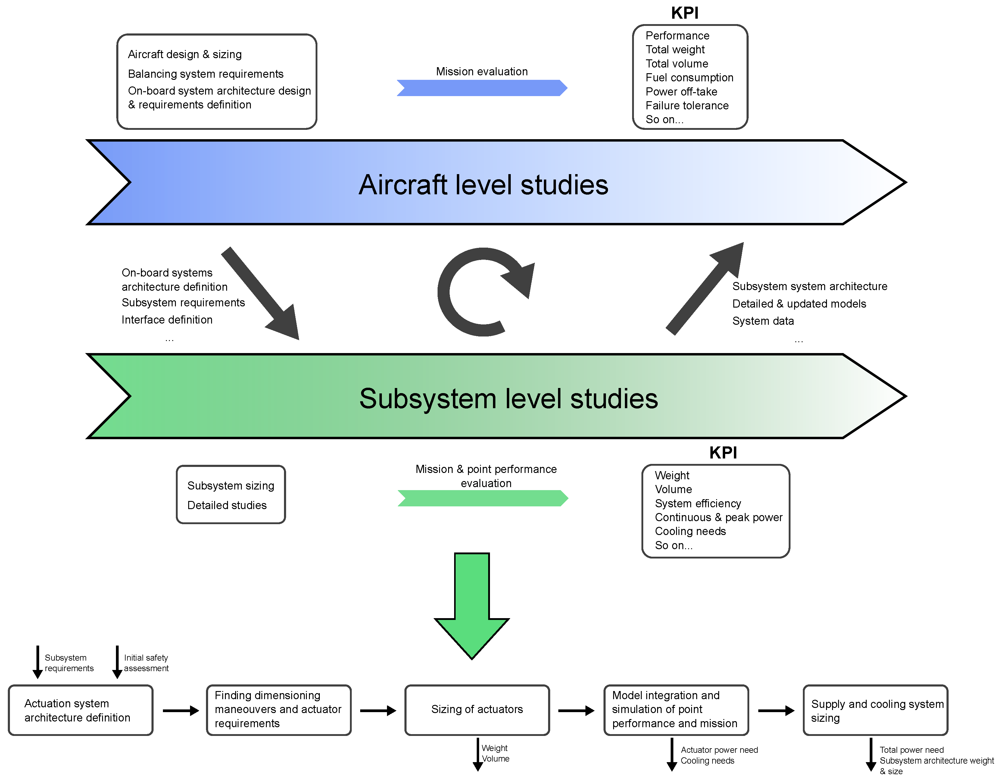
The information from this study would be fed back to the aircraft level according to the work flow in Figure 2 where the fuel burn, aircraft performance, installation effects, maintenance, safety, cost, and any other parameters can be evaluated. This process is iterated until a well-balanced design is found.

• Flight mission analysis

A flight mission is simulated, shown in Figure 17, in order to demonstrate how the power extraction and thermal characteristics can be analyzed. It shows the flight altitude and Mach number in the two top figures, the actuator position and load in the two middle figures, and the different temperatures in the bottom figures. The bottom left shows the bay temperature, which is the actuator’s surrounding temperature, and the actuator temperature for the EMA canard and inner elevon and the EHA inner elevon. The right bottom figure shows the temperature for the EHA canard for two different design options.

The aircraft spends most of the time in high altitudes where the ambient temperature is cold. The elevon actuator only operates during maneuvering and remains close to being unloaded during the cruise segments. The temperature therefore remains nearly unchanged. The canard, on the other hand, is continuously loaded, and this affects the temperature. The difference in the design is clearly seen by comparing the EMA and EHA temperatures for the canard actuator. The EMA, being a direct driven configuration, has a much larger motor and is therefore not affected nearly as much as the EHA by the load. The first design option of the EHA has a high-speed pump and therefore a much smaller motor resulting in a too-high temperature. The framework quickly allows one to change the design. By doubling the pump displacement, a larger motor is used, which results in a much lower motor temperature. The total actuator weight only increased by around 10 %. By effectively iterating the design, the framework allows one to compare several solutions to changing missions and requirements until a satisfying design is found.

The next evolution of the model would include the thermal behavior around the coil windings and the internal thermal propagation. This would require a much more detailed design of the actuator, suitable when the overall design has matured and more information is available.

6. Conclusions

This paper answers the question of how to compare different actuation system architectures in the early aircraft conceptual design phase by including the most dominant static and dynamic phenomenon of the actuation system and adjacent systems, which increases confidence in the design. A method is proposed that considers the modeling and sizing of the architectures by involving dynamic system simulation. A statistical approach using Singular Value Decomposition and regression models allows one to estimate model parameters even if very little is known about the design or requirements. The main contribution of this work is the application of the methods to a hydraulic and two electric flight control actuation systems architecture, where the actuators were modeled in a generic way that describes the static and dynamic characteristics and finally integrated in a dynamic simulation framework to size the complete architecture. The SVD modeling and analysis is used to develop a functional and characteristic model of an EMA and an EHA that allows one to estimate the weight and size, as well as functional parameters such as the inertia, torque constant, thermal characteristics, and winding resistance, where only four design input parameters have been used. The model is able to estimate the values within reasonable accuracy considering the level of detail available in the early conceptual design phase. The integration in the dynamic simulation framework is showcased in order to estimate the power and cooling needs for different missions or flight maneuvers and finally the weight and size of the architecture and its constituent components. The results not only validate the methodology for three different use cases but also highlight the different characteristics between hydraulic and electric actuation in terms of actuator weight and size, supply system weight and size, and power needs for this type of application. The trends clearly show the advantage of the high power density of hydraulic actuators compared to electric, while the opposite is true for the supply systems.