Article

Rapid SLAM Method for Star Surface Rover in Unstructured Space Environments

School of Automation and Electronic Information, Xiangtan University, Xiangtan City 411105, China
*
Author to whom correspondence should be addressed.
Aerospace 2024, 11(9), 768; https://doi.org/10.3390/aerospace11090768
Submission received: 30 July 2024 / Revised: 29 August 2024 / Accepted: 29 August 2024 / Published: 19 September 2024
(This article belongs to the Section Astronautics & Space Science)

Abstract

:
The space environment is characterized by unstructured features, sparsity, and poor lighting conditions. The difficulty in extracting features from the visual frontend of traditional SLAM methods results in poor localization and time-consuming issues. This paper proposes a rapid and real-time localization and mapping method for star chart surveyors in unstructured space environments. Improved localization is achieved using multiple sensor fusion to sense the space environment. We replaced the traditional feature extraction module with an enhanced SuperPoint feature extraction network to tackle the challenge of challenging feature extraction in unstructured space environments. By dynamically adjusting detection thresholds, we achieved uniform detection and description of image keypoints, ultimately resulting in robust and accurate feature association information. Furthermore, we minimized redundant information to achieve precise positioning with high efficiency and low power consumption. We established a star surface rover simulation system and created simulated environments resembling Mars and the lunar surface. Compared to the LVI-SAM system, our method achieved a 20% improvement in localization accuracy for lunar scenarios. In Mars scenarios, our method achieved a positioning accuracy of 0.716 m and reduced runtime by 18.682 s for the same tasks. Our approach exhibits higher localization accuracy and lower power consumption in unstructured space environments.

1. Introduction

Simultaneous Localization and Mapping (SLAM) technology enables mobile robots to navigate in motion [1]. It corrects errors in waypoint projection (inertial guidance, odometry) by incorporating observations of the surrounding scene from onboard sensors as constraints. This enables precise localization and concurrent modeling of the environment map [2]. Over the past two decades, the employment of individual perception sensors, such as lidar or cameras, has achieved remarkable success in real-time state estimation and mapping through the application of SLAM. Numerous issues have become apparent with the emergence of single-sensor systems [3]. For instance, single-vision sensors struggle to extract features in sparse textures and poor lighting conditions [4]; single-lidar sensors are prone to scene degradation in open environments [5]; and single-IMU sensors face errors caused by environmental changes [6]. Therefore, a single sensor cannot comprehensively perceive the complexities of the space environment. For the star surface rover, fully utilizing information from multiple sensors to assist in localization is paramount for its autonomous navigation [7,8]. Effectively using information from various sensors to aid in positioning is critical for autonomous navigation [9,10]. Autonomous navigation technology covers multiple key components such as SLAM (Simultaneous Localization and Mapping) and path planning, and in our current work, we mainly focus on how to stably improve the positioning accuracy of SLAM technology [11,12]. Zhang et al. proposed V-LOAM (Visual–Lidar Odometry and Mapping) based on the LOAM algorithm. It integrates monocular feature tracking and IMU measurements to provide distance prior information for lidar scan matching [13]. However, the algorithm operates on a frame-by-frame basis, lacking global consistency. To address this issue, Wang et al. proposed a loosely-coupled SLAM method that maintains a keyframe database for global pose graph optimization, ultimately enhancing global consistency [14].
The loosely coupled multi-sensor fusion SLAM method treats each sensor as a separate module to independently calculate pose information, which is then fused. However, this approach is less effective in localization performance than tightly coupled methods. Ti et al. introduced a tightly coupled framework, LVI-SAM (Tightly coupled Lidar–Visual–Inertial Odometry via Smoothing and Mapping) [15], for laser–visual–inertial odometry achieved through smoothing and mapping. It achieves high-precision and robust real-time state estimation and map construction. LVI-SAM adopts a factor graph composed of two subsystems: a visual–inertial system (VIS) and a lidar–inertial system (LIS). The star surface rover operates in an unstructured, feature-sparse environment that lacks significant structured information, such as lines and planes [16,17]. When confronted with space environments, the traditional visual–inertial system of LVI-SAM also encounters difficulties in feature extraction and feature matching failures.
Currently, mainstream visual–inertial SLAM encompasses traditional methods and deep learning-based methods [18,19,20,21]. Traditional methods primarily rely on manually designed point features for image matching and tracking. The camera pose is estimated by jointly optimizing the visual feature point reprojection error and the IMU measurement error. The visual–inertial system of LVI-SAM utilizes sparse optical flow for feature tracking. Nonlinear optimization is employed to jointly constrain visual geometry and IMU measurement errors, updating the state variables. However, reliance on point feature extraction can easily lead to feature tracking failures in poorly lit and unstructured complex space environments. Most deep learning-based methods employ end-to-end joint training on image and IMU data to directly estimate camera poses. VINet is the first visual–inertial odometry system trained using an end-to-end network, enhancing its pose estimation robustness by learning calibration errors [22]. DeepVIO achieves self-supervised end-to-end pose estimation by integrating 2D optical flow prediction and IMU preintegration networks [23]. However, end-to-end visual–inertial SLAM systems require extensive training data from diverse scenes, resulting in poor generalization capabilities. Additionally, they lack loop closure detection modules, making them unable to correct accumulated errors from long-term motion.
Within the realm of deep learning methodologies, there exists Semantic SLAM (Semantic Simultaneous Localization and Mapping) [24], a technology that builds upon the foundation of traditional SLAM by ingeniously incorporating semantic information to achieve a deeper level of environmental understanding and modeling. Semantic SLAM not only provides precise spatial localization and mapping capabilities but also possesses the ability to recognize and interpret various objects and their attributes within the environment, thereby endowing robots or intelligent systems with richer and more comprehensive environmental perception capabilities. However, despite demonstrating remarkable performance in structured scenarios, the application of Semantic SLAM faces certain limitations when confronted with unstructured scenarios. These scenarios are often characterized by complexity, variability, and unpredictability, posing numerous challenges for Semantic SLAM in handling such environments, including difficulties in object recognition and inaccuracies in map construction.
Traditional visual–inertial SLAM systems establish feature associations between images by tracking manually designed point features. ORB-SLAM2 (an Open-Source SLAM System for Monocular, Stereo and RGB-D Cameras) utilizes ORB (Oriented FAST (Features from accelerated segment test) and BRIEF (Binary Robust Independent Elementary Features)) [25] for feature extraction and matching in the visual frontend, owing to its low computational cost and rotational and scale invariance. However, it still generates a significant number of mismatches in low-texture scenes. The visual–inertial system of LVI-SAM employs Shi-Tomasi [26] to detect feature points and track them using an optical flow algorithm. However, its feature tracking performance is suboptimal in scenes with significant lighting changes. SIFT (Scale-Invariant Feature Transform) [27] exhibits high matching accuracy, but its computational cost is high, rendering real-time operation infeasible.
While manually designed point features are easily extractable and describable, their stability is low in poor lighting conditions and unstructured scenes, significantly impacting the algorithm’s robustness. GCN (Geometric Correspondence Network) [28,29] integrates convolutional networks with recurrent networks to train a geometric correspondence network for detecting keypoints and generating descriptors. Furthermore, this network supersedes the ORB feature extractor in the ORB-SLAM2 system, delivering pose estimation accuracy commensurate with the original system. Nevertheless, it exhibits a reliance on specific training scenarios.
To achieve precise positioning in unstructured space environments, we need to use multiple sensors to perceive the complex space environment. Laser sensors can provide depth information for visual sensors, while visual sensors can effectively address the environmental degradation issues of laser sensors in open space environments. However, traditional visual feature extraction methods often face difficulties in extracting features, of uneven feature extraction, and of a long feature extraction time in unstructured space environments. SuperPoint [30] employs a self-supervised network to concurrently predict keypoints and descriptors, facilitating robust feature extraction in scenarios with poor lighting conditions and unstructured features. Given SuperPoint’s robust scene adaptability, this paper proposes to enhance and integrate it as the foundational framework into the LVI-SAM visual–inertial system. By harnessing deep neural networks for feature point extraction and matching and dynamically adjusting threshold parameters, the system ensures a balanced extraction of feature points from each image frame. This approach mitigates the issue of uneven feature point extraction caused by poor scene lighting and unstructured environments. At the same time, we also need to lighten the encoding layer of SuperPoint to improve the overall efficiency of the SLAM system. So that it can consume less energy in complex space environments and complete as many space exploration and scientific research tasks as possible, our approach is as follows:
(1)
Building upon previous outstanding SLAM research, we propose a robust LVI-SAM system that leverages deep learning, further expanding upon the foundation laid by LVI-SAM. This system maintains excellent robustness and localization accuracy in the complex environments encountered on the lunar and Martian surfaces.
(2)
We introduce an enhanced SuperPoint feature extraction network model for detecting feature points and matching descriptors. This model dynamically adjusts the feature extraction threshold to achieve a balanced number of feature points, ensuring robust and reliable feature correspondences. This approach guarantees the accuracy of the optimization process at the backend of the SLAM system.
(3)
Changes in the architecture of the SuperPoint coding layer model are implemented to reduce redundant information, ensuring high efficiency and low power consumption during localization for the SLAM system.

2. System Overview

2.1. Analysis of Factors Influencing SLAM in Extraterrestrial Environments

The Moon and Mars are characterized by sparse and unstructured features, primarily plains and cratered terrain [31]. The surface of the Moon is covered with rocks and dust, while Mars’ surface is extensively covered with dunes and gravel [32]. Some regions of the Moon experience prolonged periods of dim light and harsh lighting conditions, while the lighting conditions on Mars are generally more favorable.
Laser SLAM is primarily utilized in Earth environments, focusing on the localization problem within structured scenes [33]. However, when confronted with open environments such as the lunar and Martian surfaces, scene degradation is more prone to occur, resulting in difficulties in SLAM localization. For example, in the lunar scenario, the positioning error of the Lego-LOAM laser SLAM algorithm reached 18.892 m, while in the Mars scenario, its positioning error was 5.274 m, and there was positioning trajectory drift. Current visual SLAM relies on texture and structured features, making it susceptible to lighting conditions [34]. For example, the visual SLAM algorithm ORB-SLAM2 achieved a positioning error of 3.381 m in the lunar scenario, and a positioning error of 2.426 m in the Mars scenario, with instances of positioning loss observed. The lunar and Martian environments are characterized by sparse features, disordered structures, and poor lighting conditions, ultimately leading to difficulties in feature extraction. As shown in Figure 1, the visual frontend of the visual SLAM algorithm VINS-Mono can only extract five feature points from a single frame of lunar imagery. Furthermore, incorrect feature matching may reduce the accuracy of SLAM positioning. As shown in Figure 2, the visual frontend of the visual SLAM algorithm VINS-Mono extracts 14 pairs of features from a single frame of Mars imagery, but 6 of these pairs are mismatched.
In the study of SLAM methods for extraterrestrial scenes, a detailed analysis of the factors affecting SLAM localization in such scenarios is summarized below:
(1)
The difficulty of feature extraction in unstructured and poorly lit space scenes results in low SLAM localization accuracy.
(2)
In unstructured and poorly lit space scenes, low feature matching accuracy results in diminished robustness of SLAM localization.
(3)
In harsh space environments, efficient and energy-saving SLAM algorithms are crucial for effective navigation.

2.2. Algorithm Introduction

2.2.1. The Improved LVI-SAM Overall Framework

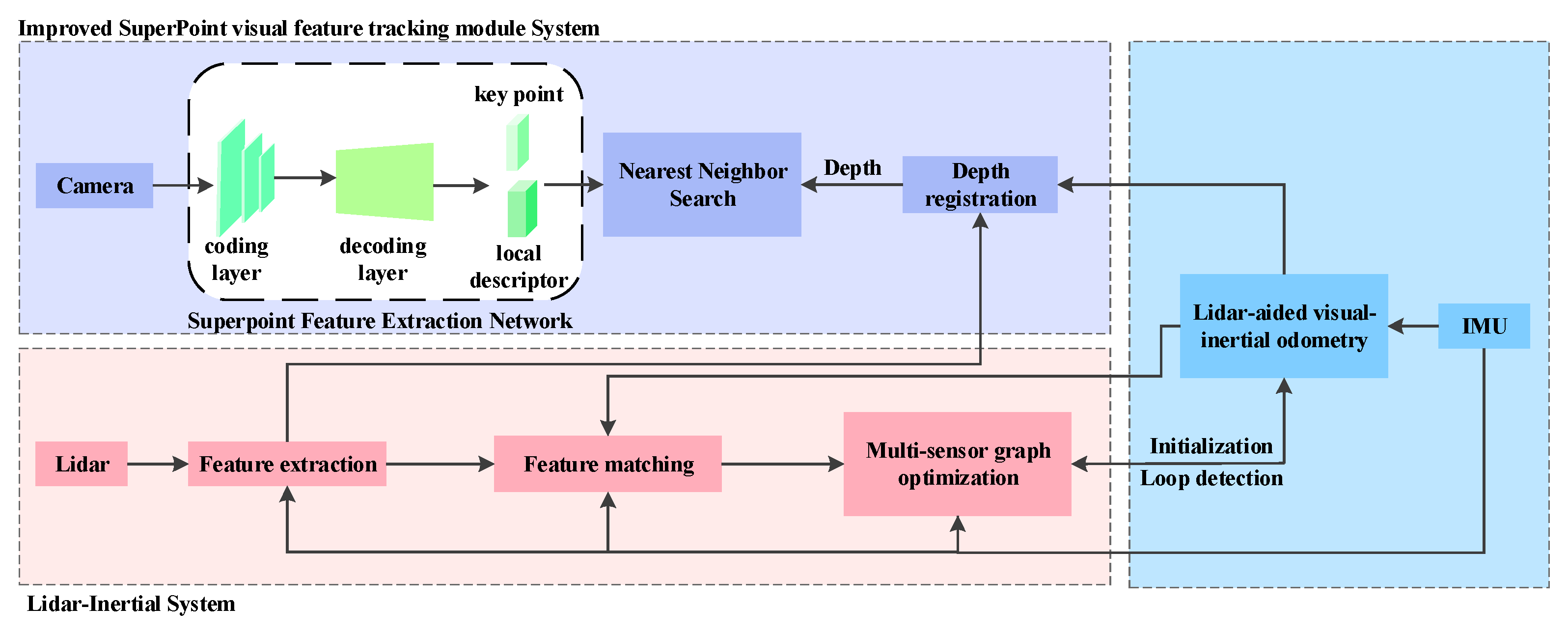
The system proposed in this paper is depicted in Figure 3. This system is constructed upon the LVI-SAM framework and comprises two subsystems: the visual–inertial system (VIS) and the lidar–inertial system (LIS) [35]. These two subsystems are designed to be closely integrated, enabling them to operate independently or collaboratively in case of a failure in one of them when adequate features are detected. The VIS subsystem performs visual feature tracking and optionally extracts feature depth utilizing lidar frames. Visual odometry, derived through optimizing errors in visual reprojection and IMU measurements, serves as an initial estimate for lidar scan matching and introduces constraints into the factor graph. After de-skewing the point cloud using IMU measurements, the LIS extracts lidar edge and planar features and matches them to a feature map maintained within a sliding window. The estimated system state in the LIS can be transmitted to the VIS to facilitate its initialization. For loop closure, candidate matches are initially identified by the VIS and further optimized by the LIS. The factor graph jointly optimizes the constraints from visual odometry, lidar odometry, IMU preintegration, and loop closure. Lastly, the optimized IMU bias terms are utilized to propagate IMU measurements for pose estimation at the IMU rate.
In the original LVI-SAM framework, the VIS system utilizes the Shi-Tomasi method for detecting feature points. Afterward, feature tracking is conducted using the LK sparse optical flow algorithm. Optical flow tracking heavily relies on the photometric invariance assumption, which may not be valid in real-world environments with varying lighting conditions.
Consequently, its feature correlation accuracy is compromised, especially in scenarios with significant illumination variations. This paper utilizes a deep convolutional network that exhibits strong robustness to lighting variations for computing feature point positions and descriptors. It can obtain consistent local descriptors even in poor lighting conditions. The enhanced SuperPoint feature extraction network output is designed to replace the LK optical flow tracking and Shi-Tomasi corner detection in the VIS. Unlike optical flow tracking, this paper employs nearest neighbor retrieval of descriptors to perform matching between feature points. Visual feature tracking yields n normalized feature point sets about adjacent images. These sets are subsequently employed to input into the backend to align IMU measurement data and formulate visual reprojection error equations.

2.2.2. Improved SuperPoint Visual Feature Tracking Module

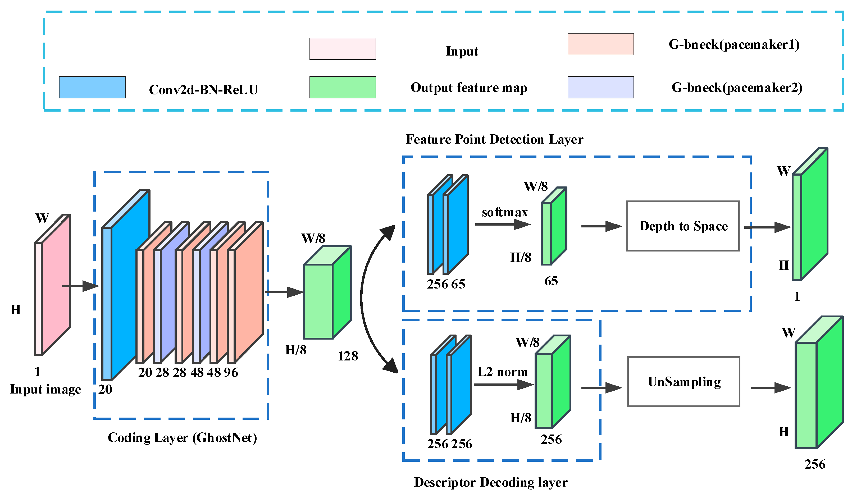
SuperPoint is a self-supervised feature extraction network framework built upon fully convolutional networks. It comprises three main components: the coding, feature point detection, and descriptor decoding layers. This architecture enables simultaneous detection and description of feature points. The coding layer of this network adopts the VGG [36] structure, which is simple yet includes a more significant number of network layers. Consequently, this results in increased computational demand and necessitates a large volume of training sample data during the training phase. Furthermore, the high-dimensional features extracted by this network often contain redundant information, which can impede the decoding process of the detection layer. This paper addresses this issue by replacing the original network framework’s VGG-like encoding layer.
The lightweight GhostNet [37] architecture, chosen for its fewer parameters and richer feature encoding information, improves the feature encoding performance of the SuperPoint network. The GhostNet architecture adopts residual block structures, using an expansion strategy followed by compression. Incorporating a series of linear operations is beneficial for expanding the receptive field of feature maps and enhancing the network’s focus on crucial information within the feature data. This approach improves the robustness of image feature extraction.
  • Coding Layer;
The GhostNet coding layer designed in this paper offers several advantages over the original VGG architecture. It uses fewer model parameters while generating richer feature maps, making the architecture more efficient and accurate in tasks such as detection and matching. As shown in Figure 4, the improved SuperPoint network framework is based on the GhostNet encoding layer. This paper’s GhostNet-based encoding layer contains the first seven layers of the original network, except for the first convolutional layer. Each layer includes a Ghost bottleneck (G-bneck). Setting the width multiplier to 1.2 ensures that the coding layer can aggregate more detailed image information. This more comprehensive channel configuration enables a richer representation of information throughout the network architecture.
2.
Feature Point Detection Layer;
The feature point detection layer performs two convolution operations on the shared feature map, transforming it from 60 × 80 × N to 60 × 80 × 65. A softmax operation is then applied to ensure that the values of the feature map are confined within the range of 0 and 1, effectively transforming the feature point detection task into a binary classification problem. A value close to 1 in the feature map signifies the presence of a valid feature point at that location. Finally, after dimensional transformation, the feature map is resized to match the dimensions of the input image. The loss function is then directly computed for the feature point detection layer.
3.
Descriptor Decoding Layer.
The original SuperPoint’s descriptor decoding layer performs three interpolation upsampling operations directly on the feature map of descriptors. The feature map values are normalized to unit length utilizing the L2 norm. This results in a dense descriptor vector with dimensions of 480 × 640 × 256. Indeed, the high dimensionality of descriptors may lead to redundant information and pose computational challenges. This paper addresses this issue by not incorporating the 3-times interpolation directly into the network model. Instead, we solely up-sample the descriptor loss function before computation. This approach significantly alleviates the computational burden during the backpropagation process.

2.2.3. Construct the Loss Function

The dense descriptor loss function of the original network has a large computation load, significantly affecting the speed of backpropagation during training. To reduce the computation load of the descriptor loss function, this paper combines the sparse descriptor loss function proposed in Reference [38], adopts pixel-level metric learning, and trains descriptors in a nearest neighbor manner. The improved SuperPoint framework simultaneously detects and describes feature points, jointly optimizing the loss functions of the feature point detection layer and the descriptor decoding layer. The network’s backpropagation loss function consists of three parts: the loss of the original feature point detector L p , the loss of the feature point detector after homography transformation L w q , and the sparse descriptor loss L d . The final loss is balanced by the weight parameter λ :
L total = ( L p + L w p ) + λ L d
  • Feature Detector Loss
When the original image I and the image I w after homography transformation H are input into the feature extraction network, two sets of corresponding feature point coordinates ( P m I , P m I w ) and local descriptor vectors ( D m I , D m I w ) can be obtained, where m represents the network output. As described in Reference [30], the loss function of the feature point detector calculates the cross-entropy loss between the predicted feature point coordinates and the actual labels. Before calculation, the pseudo-true feature point coordinates ( P G I , P G I w ) need to be converted into image feature point labels ( l G I , l G I w ) composed of ( 0 , 1 ) , where G represents the true labels.
At this point, the calculation of L p and L w q becomes a classification problem. The loss function of the feature point detector is as follows:
{ L p = 1 H c W c CrossEntropy ( P m I , l G I ) L w p = 1 H c W c CrossEntropy ( P m I w , l G I w )
In the formula W c = W / 8 ; H c = H / 8 , W represents the width of the image; H represents the height of the image.
2.
Sparse Descriptor Loss
Unlike the original SuperPoint network that uses dense descriptors, this paper replaces the dense descriptor loss function with the sparse descriptor proposed in Reference [38]. Using only the descriptors at the true label locations, the descriptor loss function is jointly determined by utilizing the triplet loss. Compared to the original dense descriptors, the computation is significantly reduced, and the model training speed is increased to 2~3 times that of the original.
Based on the actual feature point labels and the descriptor information matrix output by the network, the predicted descriptor matrix at the actual feature points is selected:
{ d m I = s e l ( D m I , l G I ) d m I w = s e l ( D m I w , l G I w )
In the equation, d m I represents the descriptor corresponding to the actual label in the original image; d m I w represents the descriptor corresponding to the valid label after homography transformation; and the selection function s e l ( D , l G ) indicates obtaining the corresponding descriptor from D :
s e l ( D , l G ) = { 0 , l G ( x , y ) = 0 D x , y , l G ( x , y ) = 1
Given the homography transformation matrix H between two known frames of images, the corresponding descriptor vectors d m I and d m I w can be derived from Equation (3). If there are N pairs of positively matched descriptor vectors, and ( x , y ) and ( x , y ) represent the corresponding positional relationships of the descriptor vectors, then the positive matching loss function can be defined as follows:
L d p ( x i , y i ) = d m I ( x i , y i ) d m I w ( x i , y i ) 2 2
By using the nearest neighbor search method, obtain M negative sample descriptor vectors d m n I w (excluding the descriptor d m I w that positively corresponds to d m I ) in the surrounding area of each pair of positively matched descriptor vectors. Then, the negative matching loss function is:
L d n ( x i , y i ) = 1 M j = 1 M ( d m I ( x i , y i ) d m n I w ( x j , y j ) 2 2 )
In the formula, i represents the number of positively matched descriptor samples; j represents the number of negative samples collected from each positively matched descriptor.
Each positive sample corresponds to M negative samples, resulting in a total of N × M negative sample pairs. A reasonable margin m d is set, which is an important indicator for measuring the similarity between descriptors. After adding the margin, the sparse descriptor loss for the entire image is as follows:
L d = 1 N i = 1 N max ( 0 , m d + L d p ( x i , y i ) L d n ( x i , y i ) )

2.2.4. Pre-Training

The training dataset for the network model is the MS-COCO dataset [39]. The self-supervised method is used for feature extraction network training, and the network model is built and trained on Pytorch. The original SuperPoint framework initializes the feature point detector using synthetic data, and generates pseudo-ground truth feature point labels for the feature detector on the dataset through homography adaptation. However, in this paper, we choose to directly use the pre-trained initialization model to extract feature point ground truth from the MS-COCO dataset in order to ensure the accuracy of the true labels of the feature points. The optimizer used is the Adam optimizer, which has a learning rate of l r = 0.0001 . Preprocess the training data by converting it to grayscale images and scaling them to 240 × 320.
Additionally, combine scale transformation, rotation transformation, and perspective transformation to construct random homography transformations, and apply these random homography transformations to the training data. The descriptor weight λ is set to 1.2, and the margin m d is set to 1.0. The model is trained for 120 K iterations on the real training data.

2.3. Fusion of Improved SuperPoint Network and LVI-SAM Visual–Inertial System

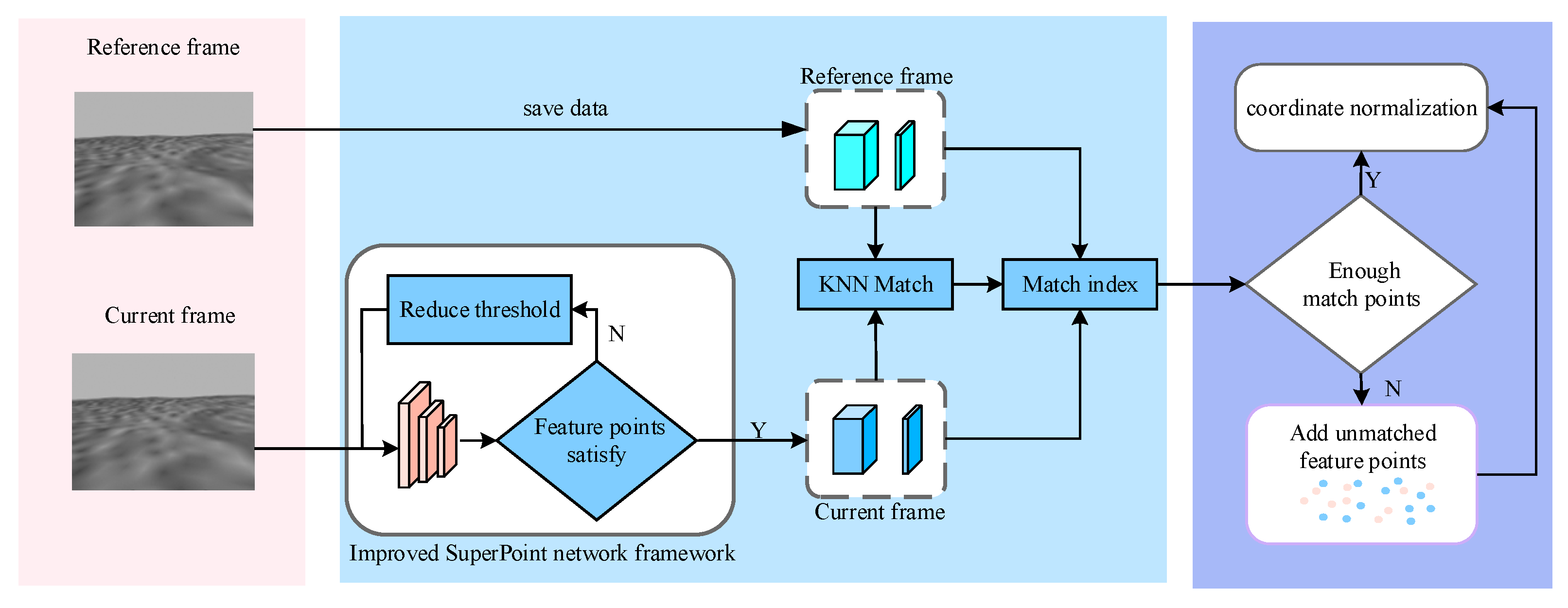
The visual feature tracking algorithm process presented in this paper is illustrated in Figure 5. The improved SuperPoint network extracts feature points from images, dynamically adjusting thresholds to ensure a balanced number of feature points on each image frame. Matching descriptors are achieved through nearest neighbor retrieval to track feature points between adjacent images and construct image feature association information. Utilizing the RANSAC algorithm to remove outliers ensures that each image frame can accurately track a specified number of feature points. To implement image feature and IMU data alignment, preintegration of IMU data and calculation of error terms, covariances, and Jacobian matrices for IMU constraints are necessary. Subsequently, visual feature observations and IMU measurement errors are published to the backend for further processing. This process ensures accurate alignment and visual and IMU data integration, resulting in robust navigation and tracking.

3. Results

3.1. Simulation Environment Setup

Real lunar and Mars DEM elevation model data were utilized to construct a simulation environment simulating the terrains of the Moon and Mars. Based on this, a simulated star surface rover was constructed [40,41]. The sensors mounted on the simulated star surface rover are composed of simulation plugins. Based on the Linux operating system (Ubuntu 20.04) and the Robot Operating System (ROS noetic) Noetic version, we have established a simulation environment on a device equipped with an Intel(R) Core(TM) i7-8550U CPU running at 1.80 GHz (actual operating frequency at 1.99 GHz). This environment utilizes real lunar and Martian DEM (Digital Elevation Model) data released by the ground application systems of China’s lunar exploration program and its first Mars exploration program, constructing simulated lunar and Martian terrains.
Elevation model data are a raster image file, typically with a file extension of .tif or .tiff, which uses grayscale values to represent surface elevation information. In this type of file, the grayscale value of each pixel corresponds to a specific elevation value, so the corresponding terrain height information can be obtained by examining the grayscale value of the pixel.
DEM elevation model data are sourced from the 50 m resolution digital elevation model data of the entire moon collected by the Chang’e-2 satellite, as well as the 3.5 m resolution digital elevation model data of Mars collected by the Tianwen-1 probe [42,43]. These data are received, processed, managed, and released by the Lunar and Deep Space Exploration Science Application Center of the National Astronomical Observatories, Chinese Academy of Sciences. This center is the construction unit of the ground application system for lunar and planetary exploration projects, and it is also one of the five major systems for China’s major national projects, including the Chinese Lunar Exploration Program and China’s first Mars exploration mission. The ground application system has successfully completed previous exploration missions for the first, second, and third phases of the lunar exploration program and is currently executing the Chang’e-4 mission and the first Mars exploration mission.
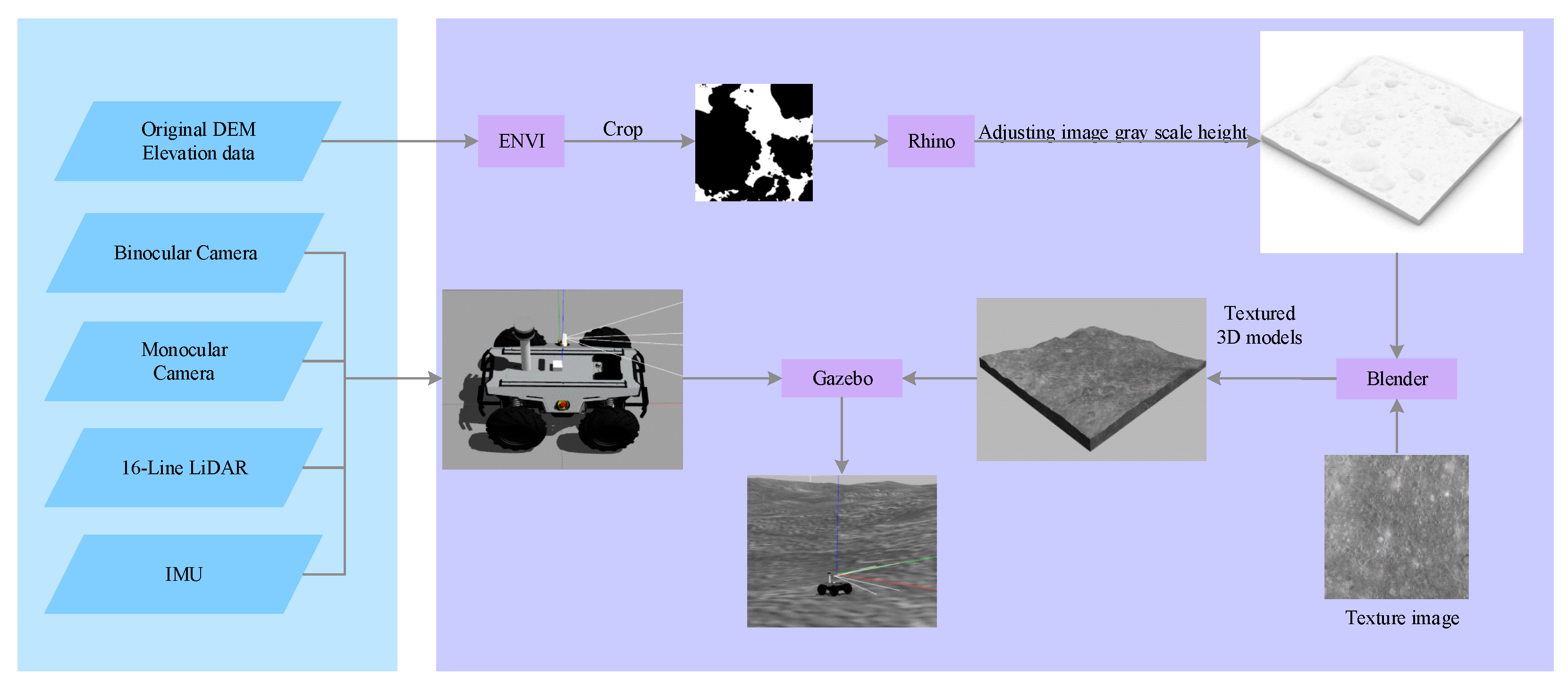
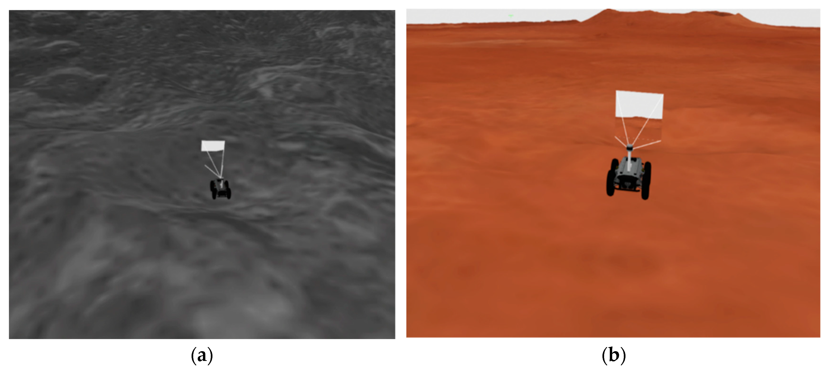
While modeling the three-dimensional terrain of extraterrestrial bodies, a series of software, including ENVI 5.6, Rhino 7, Blender 3.6, and Gazebo 11, was utilized to transform the two-dimensional elevation data into vivid and realistic three-dimensional terrain models. The modeling process is depicted in Figure 6. The simulation models of the lunar and Martian terrains are illustrated in Figure 7. The detailed steps of the modeling process are presented below:
(1)
Initially, the elevation data should be imported into ENVI software for cropping. Crop the elevation map to 2500 × 2500 pixels to prevent complications associated with loading massive elevation datasets.
(2)
Import the cropped elevation data into Rhino software to adjust the grayscale height of the image and export it to the DAE format for the three-dimensional model. Rhino software converts the grayscale values from the original elevation map into height values in the three-dimensional model.
(3)
Import the DAE 3D model into Blender software, apply texture maps, and export the textured DAE 3D model. This step facilitates the more effective simulation of texture information on the surface of extraterrestrial bodies.
(4)
A URDF (Unified Robot Description Format) model was constructed, comprising wheels, chassis, transmission system, control module, monocular camera, binocular camera, 16-line LiDAR (Light Detection and Ranging), and Inertial Measurement Unit (IMU).
In the simulation system, the Robot Operating System (ROS) packages, nodes, and plugins used are as follows:
(1)
scout_gazebo: This package contains the Unified Robot Description Format (URDF) file, world files, and configurations for the simulated rover. The URDF file is used to describe the rover’s physical structure, including links, joints, etc.
(2)
xacro: This is a ROS package for handling XML macros (XACRO). It allows you to write reusable rover descriptions, making URDF files more concise and modular.
(3)
gazebo_ros: This is an interface software package between the Gazebo simulation environment and ROS. It allows you to load and run ROS simulated rovers in Gazebo.
(4)
spawn_model: This is a node in the gazebo_ros package used to load simulated rover models into the Gazebo simulation environment. It retrieves the rover’s URDF description from the robot_description parameter on the parameter server and loads it into Gazebo.
(5)
joint_state_publisher and robot_state_publisher: These two nodes are used to publish the robot’s joint states and the complete rover state for visualization in tools such as RViz.
(6)
rviz: This is the executable file for RViz, used to visualize data from ROS topics.
(7)
libgazebo_ros_camera.so: A plugin for simulating camera sensors.
(8)
libgazebo_ros_depth_camera.so: A plugin for simulating depth camera sensors.
(9)
libgazebo_ros_imu.so: A plugin for simulating IMU sensors.
(10)
libgazebo_ros_laser.so: A plugin for simulating laser sensors.
(11)
libgazebo_ros_multicamera.so: A plugin for simulating multicamera sensors.
(12)
libgazebo_ros_control.so: A plugin that provides control capabilities for interacting with the Gazebo simulation environment.
(13)
libgazebo_ros_diff_drive.so: A plugin for simulating differential drive robots.

3.2. Visual Feature Extraction and Matching Comparative Experiment

3.2.1. Experimental Data and Algorithms

A comparison of the performance of three visual feature tracking modules in simulated lunar and Mars scenarios is conducted. Their strengths and weaknesses in feature extraction, matching, and efficiency are evaluated. The aim is to determine which module performs best in these simulated environments and identify areas for improvement.
(1)
ST + LK represents Shi-Tomasi + LK, the visual tracking method initially employed by the LVI-SAM system.
(2)
SP + KNN represents the deep learning method SuperPoint combined with K-Nearest Neighbor.
(3)
Our method represents an improved version of SuperPoint based on the GhostNet encoding layer combined with K-Nearest Neighbor.
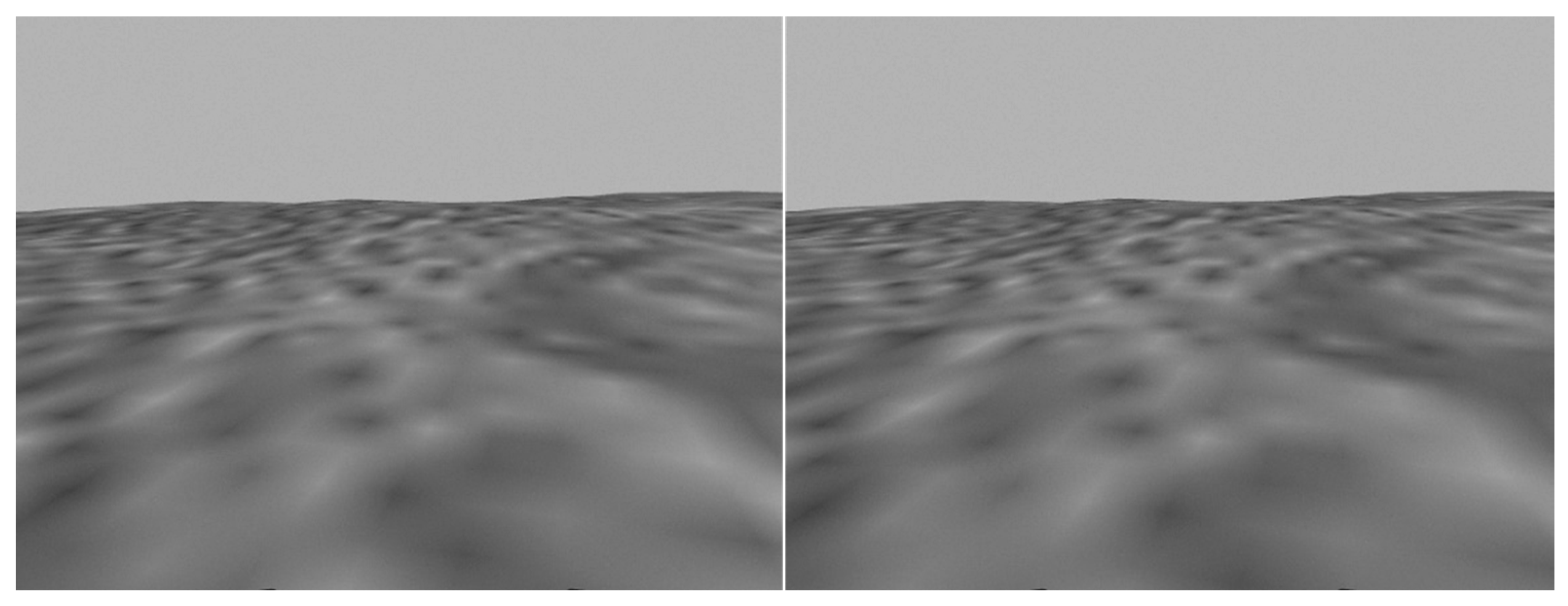
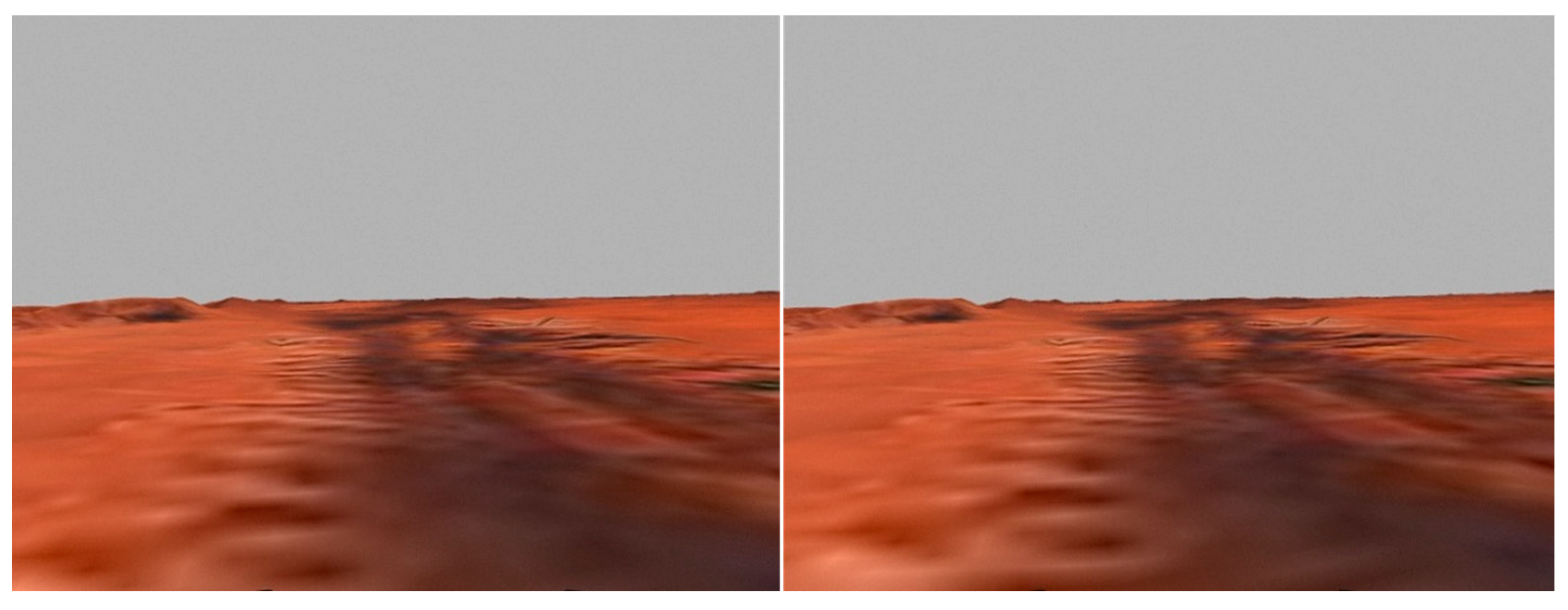
The image pairs selected from simulated lunar and Mars environments, captured by the visual sensors, are presented in Figure 8 and Figure 9.

3.2.2. Experimental Analysis

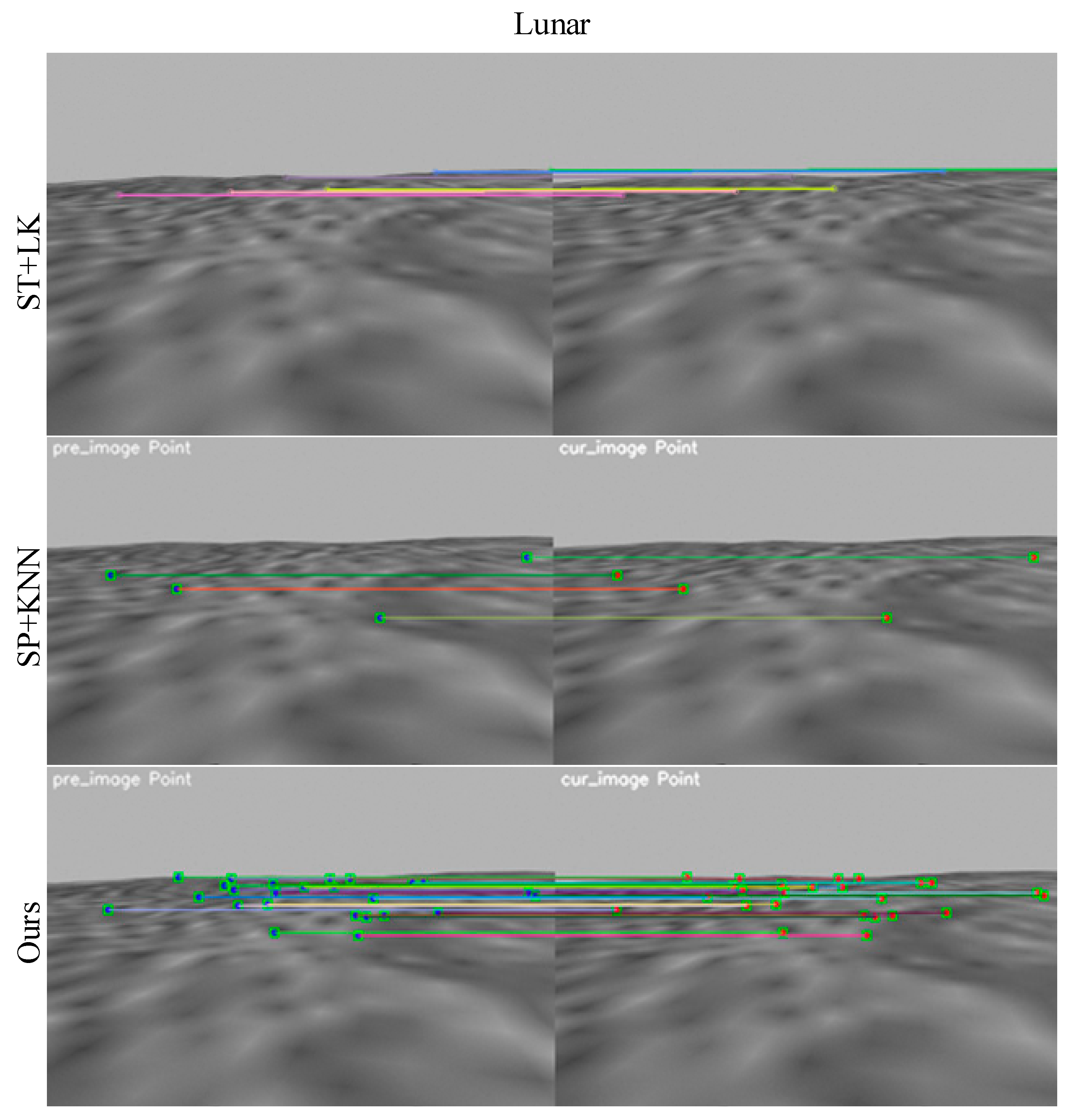
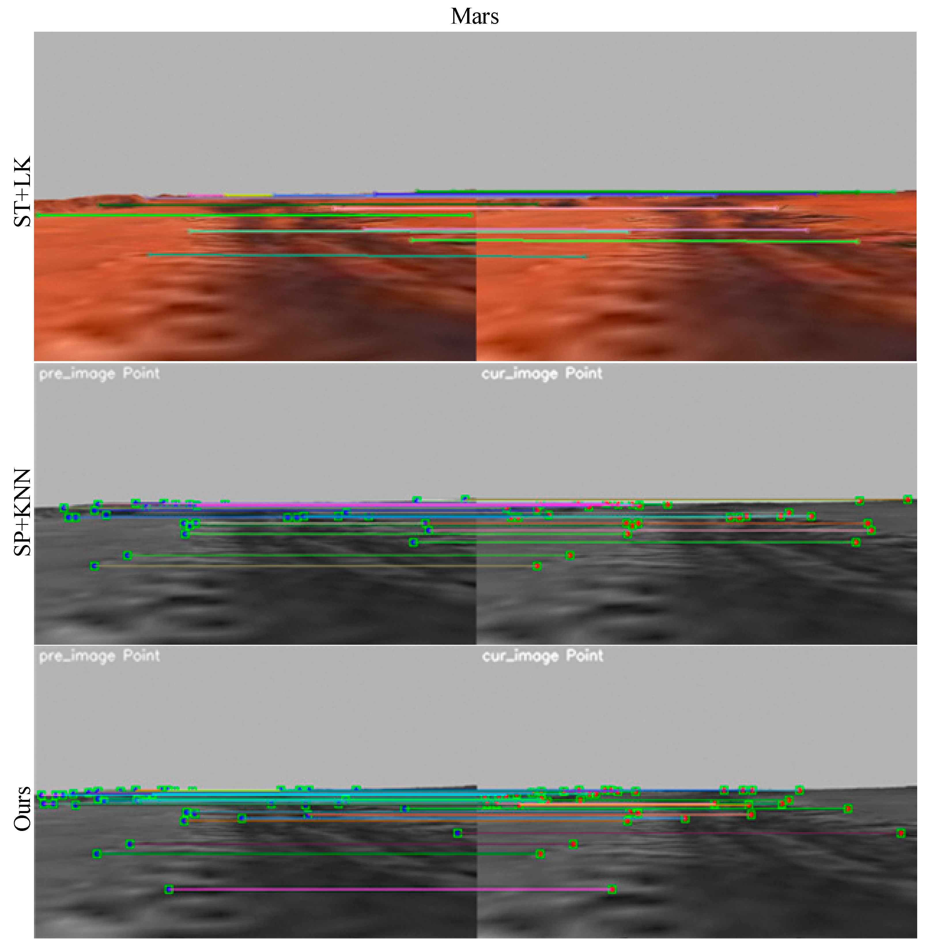
Figure 10 and Figure 11 display the outcomes of extracting and matching visual features using three visual feature tracking modules on simulated pairs of lunar and Mars images. According to Figure 10, our method, which is the SuperPoint method enhanced with the GhostNet encoding layer and combined with the K-Nearest Neighbor approach, extracts the most feature points. Additionally, it is observable that the original visual tracking method, Shi-Tomasi + LK (ST + LK), extracts very few features. Furthermore, the associated features in the matching process are minimal, indicating potential mismatches. Our method, integrating the GhostNet encoding layer enhancement for SuperPoint alongside the K-Nearest Neighbor approach, demonstrates a significant improvement in feature extraction and matching capabilities. Furthermore, the features extracted and matched by the three visual feature tracking algorithms are notably more prevalent in the Mars image pair than in the lunar ones.
Table 1 compares the number of extracted features, mismatched features, and runtime among three visual feature tracking modules. The top-performing algorithms are denoted in red. According to Table 1, the original visual tracking method Shi-Tomasi + LK (ST + LK) exhibits a low number of feature extractions and a high number of mismatches. On the Lunar image pair, only seven feature points were extracted, among which one feature point was incorrectly tracked by the optical flow method, resulting in a correct matching rate of 85.7%. On the Mars image pair, only 14 feature points were extracted, among which 6 feature points were incorrectly tracked by the optical flow method, leading to a high error matching rate of 42.9%. While LK optical flow tracks feature quickly, the low number of extractions and high number of mis-tracked features result in poor localization accuracy of SLAM in lunar and Mars scenes. Despite not having mismatching issues in feature matching, the deep learning method SuperPoint + K-Nearest Neighbor (SP + KNN) still exhibits few feature extractions. SP + KNN only extracted four feature points on the lunar image pair, and the runtime of SP + KNN on the Mars image pair was 18.978 s. The long runtime and high energy consumption make SP + KNN unsuitable for exploration tasks on harsh planetary surfaces. Our method, which is based on GhostNet encoding-enhanced SuperPoint with K-Nearest Neighbor, exhibits the highest number of feature extractions. It extracted 25 feature points from the lunar image pair and 38 from the Mars image pair, significantly higher than ST + LK and SP + KNN. Moreover, our method achieves a 100% correct matching rate. The runtime on the lunar image pair was 0.292 s, and on the Mars image pair, it was 0.296 s. This makes our method more energy-efficient than SP + KNN. Our proposed method demonstrates significant feature extraction, matching, and high-power and low-power positioning advantages. It has the potential to significantly benefit SLAM localization in the future.

3.3. Simulation-Based SLAM Comparative Experiment

3.3.1. Experimental Data and Algorithms

We recorded bag data of the simulated star surface rover in the simulated lunar and Mars environments, respectively. The bag data include odometry, IMU, monocular camera, stereo camera, and 16-line lidar messages. We compared mainstream laser SLAM algorithms, including Lego-LOAM, the stereo module of ORB-SLAM2, the multi-sensor fusion SLAM algorithm LVI-SAM without the SuperPoint module, and our improved LVI-SAM-SuperPoint algorithm, using the SLAM accuracy evaluation tool (EVO 1.12) to directly assess the error between each algorithm and the ground truth trajectory.

3.3.2. Experiment Analysis

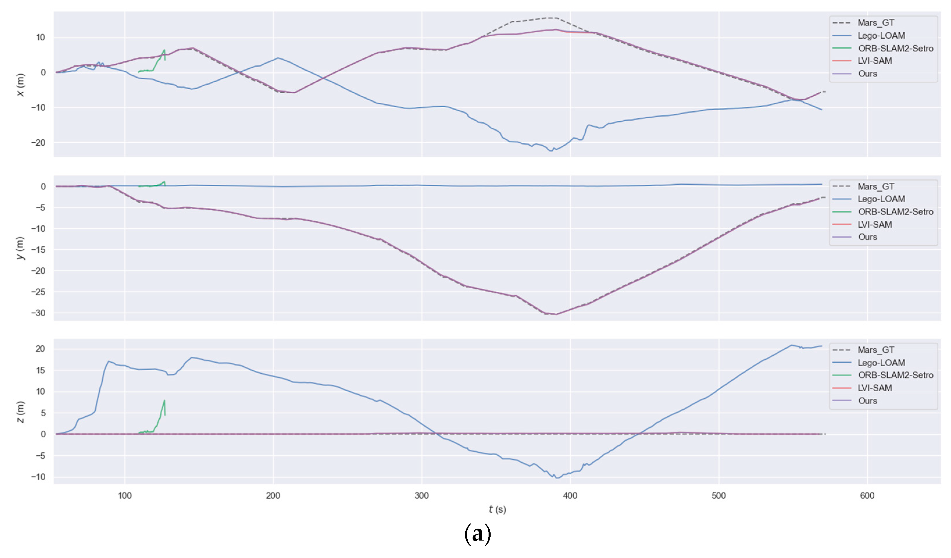
Figure 12 illustrates the synchronized procedure of localization and mapping of the simulated star surface rover within the simulated lunar environment, accompanied by the resultant trajectory. As seen in Figure 12, in both simulated lunar and Mars environments, our method is the closest to the actual trajectory of the rover, followed by LVI-SAM. Lego-LOAM completely deviates from the actual trajectory. Most of the location information is lost in ORB-SLAM2.
Figure 13 illustrates the trajectory errors generated by the rover using different methods in simulated lunar and Martian environments. As shown in the figure, our method performs best on the actual trajectory of the rover on the simulated planetary surface, followed closely by LVI-SAM. In comparison, the trajectory of Lego-LOAM completely deviates from the actual path. ORB-SLAM2, on the other hand, loses position information for most of the time and only retains partial trajectory information during the 100–200 s timeframe in the Martian environment and the 600–700 s timeframe in the lunar environment.
Table 2 displays the localization errors of four SLAM methods in simulated lunar and Mars scenarios. The best-performing algorithms are highlighted in red. As shown in Table 2, our method exhibits the best performance in terms of root mean square error (RMSE) and mean error among all algorithms. In the lunar scenario, the positioning error of Lego-LOAM is 18.892 m, ORB-SLAM2 has an error of 3.381 m, LVI-SAM has an error of 3.617 m, while our improved method achieves an accuracy of 2.894 m. Compared to LVI-SAM, the positioning accuracy improved by 0.723 m, with a percentage increase of 20%. In the Mars scenario, the positioning error for Lego-LOAM was 5.274 m. For ORB-SLAM2, it was 2.426 m, and for LVI-SAM, it was 1.003 m. Our improved method achieved an accuracy of 0.716 m. The positioning accuracy of LVI-SAM was improved by 0.054 m, with a percentage improvement of 7%. The positioning accuracy on Mars is much higher than on the lunar surface, confirming the experimental analysis mentioned in Section 3.2, which noted that more feature points were extracted on Mars compared to the lunar surface. The reason is that the poor lighting conditions on the lunar surface are not conducive to feature extraction by the visual feature tracking module. The various evaluation indicators in Table 2 indicate that our improved method significantly improves positioning accuracy in the context of feature-scarce, poor lighting, and unstructured planetary environments.

4. Discussion

This paper introduces an enhanced LVI-SAM system leveraging deep learning techniques. The system integrates an improved SuperPoint network into the LVI-SAM framework, specifically within the visual processing component. Compared to recent traditional LVI-SAM systems, our system integrates the feature extraction network into the visual processing frontend, significantly enhancing localization accuracy in challenging scenarios. Furthermore, by comparing different encoding layers of the SuperPoint network, it is verified that the network based on the fully convolutional encoding layer performs better in feature extraction, especially in homography matrix estimation. At the same time, we have optimized the model architecture of the SuperPoint encoding layer, reducing redundant information and ensuring high efficiency and low power consumption in the SLAM system for localization. This integration has notably improved the system’s positioning accuracy in challenging environments with poor illumination and unstructured features. The SuperPoint network based on GhostNet exhibited superior feature extraction performance when comparing three visual feature modules. The proposed system significantly improved localization accuracy in simulated lunar and Mars scenarios. In the lunar scenario, the localization accuracy of Lego-LOAM is 18.892 m, while that of ORB-SLAM2 is 3.381 m, and LVI-SAM achieves a localization accuracy of 3.617 m. After improvement, the localization accuracy of LVI-SAM-SuperPoint, which incorporates SuperPoint, is enhanced to 2.894 m, representing an improvement of 0.723 m compared to LVI-SAM without SuperPoint, with an increase percentage of 20%. In the Mars scenario, Lego-LOAM achieves a localization accuracy of 5.274 m, ORB-SLAM2 achieves 2.426 m, and LVI-SAM achieves 1.003 m. Similarly, after improvement, the localization accuracy of LVI-SAM-SuperPoint is boosted to 0.716 m, showing an improvement of 0.054 m compared to LVI-SAM without SuperPoint, with an increase percentage of 7%. These results highlight the effectiveness of the proposed deep learning-based LVI-SAM system in enhancing feature extraction and localization robustness during planetary exploration missions. Our innovative method significantly differs from recent deep learning-based SLAM approaches such as SplaTAM (Splat, Track, & Map 3D Gaussians for Dense RGB-D SLAM) [44] and Gaussian-SLAM (Photo-realistic Dense SLAM with Gaussian Splatting) [45]. Both of these methods use 3D Gaussian distributions as the underlying map representation and achieve dense RGB-D SLAM through an online tracking and mapping framework, significantly enhancing camera pose estimation, map construction, and novel view synthesis performance while enabling real-time rendering of high-resolution dense 3D maps. However, in environments with insufficient lighting and color information, as well as large featureless areas, such as the Moon and Mars, these methods may not effectively perform camera tracking and scene reconstruction. Future research efforts will concentrate on integrating deep learning methodologies into the feature extraction module of LVI-SAM’s laser module, aiming to further enhance the extraction of robust and stable feature points, ultimately elevating the overall localization accuracy of the LVI-SAM algorithm.

Author Contributions

Conceptualization, Z.Z. and Y.C.; methodology, Z.Z.; software, Y.C.; validation, Z.Z., Y.C. and L.B.; formal analysis, Z.Z.; investigation, Y.C.; resources, J.Y.; data curation, L.B.; writing—original draft preparation, Y.C.; writing—review and editing, Z.Z.; visualization, Y.C.; supervision, L.B.; project administration, J.Y.; funding acquisition, Z.Z. All authors have read and agreed to the published version of the manuscript.

Funding

This research was funded by the General Program of Hunan Provincial Science and Technology Department (No. 2022JJ30561) and the Open Topic of the Space Trusted Computing and Electronic Information Technology Laboratory of Beijing Control Engineering Institute (No. OBCandETL-2022-04).

Data Availability Statement

The training data presented in this study are available in the COCO dataset repository at https://cocodataset.org/, accessed on 2 December 2022. These data were derived from the following resources available in the public domain: https://cocodataset.org/, accessed on 2 December 2022. The simulated data presented in this study are available at the request of the corresponding author due to the author’s ongoing innovative work based on this dataset. Once this additional work is completed, the data will be made openly available.

Acknowledgments

I would like to express my gratitude to the Hunan Provincial Science and Technology Department for its generous funding and support of the general project (No. 2022JJ30561), which has provided an important material foundation and motivation for my research work. At the same time, I would also like to thank the Open Topic (No. OBCandETL-2022-04) of the Space Trusted Computing and Electronic Information Technology Laboratory of the Beijing Institute of Control for its strong support and assistance to this research. The support of this topic not only provided me with valuable research resources but also greatly promoted my exploration and progress in related fields.

Conflicts of Interest

The authors declare no conflicts of interest.

References

  1. Mur-Artal, R.; Montiel, J.M.M.; Tardos, J.D. ORB-SLAM: A Versatile and Accurate Monocular SLAM System. IEEE Trans. Robot. 2015, 31, 1147–1163. [Google Scholar] [CrossRef]
  2. Qin, T.; Peiliang, L.; Shaojie, S. VINS-Mono: A Robust and Versatile Monocular Visual-Inertial State Estimator. IEEE Trans. Robot. 2018, 34, 1004–1020. [Google Scholar] [CrossRef]
  3. Li, Q.; Queralta, J.P.; Gia, T.N.; Zou, Z.; Westerlund, T. Multi-Sensor Fusion for Navigation and Mapping in Autonomous Vehicles: Accurate Localization in Urban Environments. Unmanned Syst. 2020, 8, 229–237. [Google Scholar] [CrossRef]
  4. Shamwell, E.J.; Leung, S.; Nothwang, W.D. Vision-aided absolute trajectory estimation using an unsupervised deep network with online error correction. In Proceedings of the 2018 IEEE/RSJ International Conference on Intelligent Robots and Systems (IROS), Madrid, Spain, 1–5 October 2018. [Google Scholar]
  5. Shan, T.; Englot, B. LeGO-LOAM: Lightweight and Ground-Optimized Lidar Odometry and Mapping on Variable Terrain. In Proceedings of the 2018 IEEE/RSJ International Conference on Intelligent Robots and Systems (IROS), Madrid, Spain, 1–5 October 2018. [Google Scholar]
  6. Kang, H.; An, J.; Lee, J. IMU-Vision based Localization Algorithm for Lunar Rover. In Proceedings of the 2019 IEEE/ASME International Conference on Advanced Intelligent Mechatronics (AIM), Hong Kong, China, 8–12 July 2019. [Google Scholar]
  7. Hou, Y.; Wang, G.C. Research on Mars Surface Image Visual Feature Extraction Algorithm. In Proceedings of the 2013 3rd International Conference on Advanced Materials and Engineering Materials 2013 (ICAMEM 2013), Singapore, 14–15 December 2013. [Google Scholar]
  8. Cao, F.; Wang, R. Study on Stereo Matching Algorithm for Lunar Rover Based on Multi-feature. In Proceedings of the 2010 International Conference on Innovative Computing and Communication and 2010 Asia-Pacific Conference on Information Technology and Ocean Engineering, Macau, China, 30–31 January 2010. [Google Scholar]
  9. Lin, J.; Zheng, C.; Xu, W.; Zhang, F. R2 LIVE: A Robust, Real-time, LiDAR-Inertial-Visual tightly-coupled state Estimator and mapping. IEEE Robot. Autom. Lett. 2021, 6, 7469–7476. [Google Scholar] [CrossRef]
  10. Zuo, X.; Yang, Y.; Geneva, P.; Lv, J.; Liu, Y.; Huang, G.; Pollefeys, M. LIC-Fusion 2.0: LiDAR-Inertial-Camera Odometry with Sliding-Window Plane-Feature Tracking. In Proceedings of the 2020 IEEE/RSJ International Conference on Intelligent Robots and Systems (IROS), Las Vegas, NV, USA, 24 October 2020–24 January 2021. [Google Scholar]
  11. Guan, W.; Wang, K. Autonomous Collision Avoidance of Unmanned Surface Vehicles Based on Improved A-Star and Dynamic Window Approach Algorithms. IEEE Intell. Transp. Syst. Mag. 2023, 15, 36–50. [Google Scholar] [CrossRef]
  12. Alamri, S.; Alamri, H.; Alshehri, W.; Alshehri, S.; Alaklabi, A.; Alhmiedat, T. An Autonomous Maze-Solving Robotic System Based on an Enhanced Wall-Follower Approach. Machines 2023, 11, 249. [Google Scholar] [CrossRef]
  13. Zhang, J.; Singh, S. Visual-lidar odometry and mapping: Low-drift, robust, and fast. In Proceedings of the 2015 IEEE International Conference on Robotics and Automation (ICRA), Seattle, WA, USA, 26–30 May 2015. [Google Scholar]
  14. Wang, Z.; Zhang, J.; Chen, S.; Yuan, C.; Zhang, J.; Zhang, J. Robust High Accuracy Visual-Inertial-Laser SLAM System. In Proceedings of the 2019 IEEE/RSJ International Conference on Intelligent Robots and Systems (IROS), Macau, China, 3–8 November 2019. [Google Scholar]
  15. Shan, T.; Englot, B.; Ratti, C.; Rus, D. LVI-SAM: Tightly-coupled Lidar-Visual-Inertial Odometry via Smoothing and Mapping. In Proceedings of the 2021 IEEE International Conference on Robotics and Automation (ICRA), Xi’an, China, 30 May–5 June 2021. [Google Scholar]
  16. Gao, X.; Zhang, T. Unsupervised learning to detect loops using deep neural networks for visual SLAM system. Auton. Robot. 2017, 41, 1–18. [Google Scholar] [CrossRef]
  17. Wang, Y.; Zhang, W.; An, P. A Survey of Simultaneous Localization and Mapping on Unstructured Lunar Complex Environment. J. Zhengzhou Univ. (Eng. Sci.) 2018, 39, 45–50. [Google Scholar]
  18. Li, R.; Wang, S.; Gu, D. DeepSLAM: A Robust Monocular SLAM System with Unsupervised Deep Learning. IEEE Trans. Ind. Electron. 2020, 68, 3577–3587. [Google Scholar] [CrossRef]
  19. Zhang, Q.; Li, C. Semantic slam for mobile robots in dynamic environments based on visual camera sensors. Meas. Sci. Technol. 2023, 34, 085202. [Google Scholar] [CrossRef]
  20. Wang, J.; Shim, V.A.; Yan, R.; Tang, H.; Sun, F. Automatic Object Searching and Behavior Learning for Mobile Robots in Unstructured Environment by Deep Belief Networks. IEEE Trans. Cogn. Dev. Syst. 2018, 11, 395–404. [Google Scholar] [CrossRef]
  21. Baheti, B.; Innani, S.; Gajre, S.; Talbar, S. Eff-UNet: A Novel Architecture for Semantic Segmentation in Unstructured Environment. In Proceedings of the 2020 IEEE/CVF Conference on Computer Vision and Pattern Recognition Workshops (CVPRW), Seattle, WA, USA, 14–19 June 2020. [Google Scholar]
  22. Clark, R.; Wang, S.; Wen, H.; Markham, A.; Trigoni, N. Vinet: Visual-inertial odometry as a sequence-to-sequence learning problem. In Proceedings of the Thirty-First AAAI Conference on Artificial Intelligence (AAAI-17), San Francisco, CA, USA, 4–9 February 2017. [Google Scholar]
  23. Han, L.; Lin, Y.; Du, G.; Lian, S. Deepvio: Self-supervised deep learning of monocular visual inertial odometry using 3D geometric constraints. In Proceedings of the 2019 IEEE/RSJ International Conference on Intelligent Robots and Systems (IROS), Macau, China, 3–8 November 2019. [Google Scholar]
  24. Alqobali, R.; Alshmrani, M.; Alnasser, R.; Rashidi, A.; Alhmiedat, T.; Alia, O.M. A Survey on Robot Semantic Navigation Systems for Indoor Environments. Appl. Sci. 2023, 14, 89. [Google Scholar] [CrossRef]
  25. Rublee ERabaud VKonolige, K.; Bradski, G.R. ORB: An efficient alternative to SIFT or SURF. In Proceedings of the 2011 International Conference on Computer Vision, Barcelona, Spain, 6–13 November 2011. [Google Scholar]
  26. Shi, J.; Tomasi, C. Good Features to Track. In Proceedings of the IEEE Conference on Computer Vision & Pattern Recognition, Seattle, WA, USA, 21–23 June 1994; Volume 600. [Google Scholar]
  27. Lowe, D.G. Object recognition from local scale-invariant features. In Proceedings of the IEEE International Conference on Computer Vision, Kerkyra, Greece, 20–27 September 1999. [Google Scholar]
  28. Tang, J.; Folkesson, J.; Jensfelt, P. Geometric correspondence network for camera motion estimation. IEEE Robot. Autom. Lett. 2018, 3, 1010–1017. [Google Scholar] [CrossRef]
  29. Tang, J.; Ericson, L.; Folkesson, J.; Jensfelt, P. Gcnv2: Efficient correspondence prediction for real-time slam. IEEE Robot. Autom. Lett. 2019, 4, 3505–3512. [Google Scholar] [CrossRef]
  30. DeTone, D.; Malisiewicz, T.; Rabinovich, A. SuperPoint: Self-Supervised Interest Point Detection and Description. In Proceedings of the 2018 IEEE/CVF Conference on Computer Vision and Pattern Recognition Workshops (CVPRW), Salt Lake City, UT, USA, 18–22 June 2018. [Google Scholar]
  31. Heiken, G.; Vaniman, D.; French, B.M. (Eds.) Lunar Sourcebook—A User’s Guide to the Moon; Cambridge University Press: Cambridge, UK, 1991. [Google Scholar]
  32. Murchie, S.; Arvidson, R.; Bedini, P.; Beisser, K.; Bibring, J.; Bishop, J.; Boldt, J.; Cavender, P.; Choo, T.; Clancy, R.T.; et al. Compact Reconnaissance Imaging Spectrometer for Mars (CRISM) on Mars Reconnaissance Orbiter (MRO). J. Geophys. Res. Atmos. 2007, 112, E05S03. [Google Scholar] [CrossRef]
  33. Gonzalez, M.; Marchand, E.; Kacete, A.; Royan, J. S3LAM: Structured Scene SLAM. arXiv 2021, arXiv:2109.07339. [Google Scholar]
  34. Shao, W.; Vijayarangan, S.; Li, C.; Kantor, G. Stereo Visual Inertial LiDAR Simultaneous Localization and Mapping. In Proceedings of the 2019 IEEE/RSJ International Conference on Intelligent Robots and Systems (IROS), Macau, China, 3–8 November 2019. [Google Scholar]
  35. Shan, T.; Englot, B.; Meyers, D.; Wang, W.; Ratti, C.; Rus, D. LIO-SAM: Tightly-coupled Lidar Inertial Odometry via Smoothing and Mapping. In Proceedings of the 2020 IEEE/RSJ International Conference on Intelligent Robots and Systems (IROS), Las Vegas, NV, USA, 24 October 2020–24 January 2021. [Google Scholar]
  36. Simonyan, K.; Zisserman, A. Very Deep Convolutional Networks for Large-Scale Image Recognition. arXiv 2014, arXiv:1409.1556. [Google Scholar]
  37. Han, K.; Wang, Y.; Tian, Q.; Guo, J.; Xu, C.; Xu, C. GhostNet: More Features from Cheap Operations. In Proceedings of the 2020 IEEE/CVF Conference on Computer Vision and Pattern Recognition (CVPR), Seattle, WA, USA, 13–19 June 2020. [Google Scholar]
  38. Jau, Y.Y.; Zhu, R.; Su, H.; Chandraker, M. Deep keypoint-based camera pose estimation with geometric constraints. In Proceedings of the 2020 IEEE/RSJ International Conference on Intelligent Robots and Systems (IROS), Las Vegas, NV, USA, 24 October 2020–24 January 2021. [Google Scholar]
  39. Lin, T.-Y.; Maire, M.; Belongie, S.; Hays, J.; Perona, P.; Ramanan, D.; Dollár, P. Microsoft COCO: Common Objects in Context. In Computer Vision—ECCV 2014. (ECCV 2014). Lecture Notes in Computer Science; Fleet, D., Pajdla, T., Schiele, B., Tuytelaars, T., Eds.; Springer: Cham, Switzerland, 2014; Volume 8693. [Google Scholar]
  40. Ma, X.; Chen, M.; Hu, T.; Kang, Z.; Xiao, M. Study on the Degradation Pattern of Impact Crater Populations in Yutu-2’s Rovering Area. Remote Sens. 2024, 16, 2356. [Google Scholar] [CrossRef]
  41. Chekakta, Z.; Zenati, A.; Aouf, N.; Dubois-Matra, O. Robust deep learning LiDAR-based pose estimation for autonomous space landers. Acta Astronaut. 2022, 201, 59–74. [Google Scholar] [CrossRef]
  42. Catanoso, D.; Chakrabarty, A.; Fugate, J.; Naal, U.; Welsh, T.M.; Edwards, L.J. OceanWATERS Lander Robotic Arm Operation. In Proceedings of the 2021 IEEE Aerospace Conference, Big Sky, MT, USA, 6–13 March 2021. [Google Scholar]
  43. Ji, J.; Huang, X. Tianwen-1 releasing first colored global map of Mars. Chin. Sci. Phys. Mech. Astron. 2023, 66, 289533. [Google Scholar] [CrossRef]
  44. Keetha, N.; Karhade, J.; Jatavallabhula, K.M.; Yang, G.; Scherer, S.; Ramanan, D.; Luiten, J. SplaTAM: Splat, Track & Map 3D Gaussians for Dense RGB-D SLAM. In Proceedings of the IEEE/CVF Conference on Computer Vision and Pattern Recognition (CVPR), Seattle, WA, USA, 17–21 June 2024. [Google Scholar]
  45. Yugay, V.; Li, Y.; Gevers, T.; Oswald, M.R. Gaussian-SLAM: Photo-realistic Dense SLAM with Gaussian Splatting. arXiv 2023, arXiv:2312.10070. [Google Scholar]
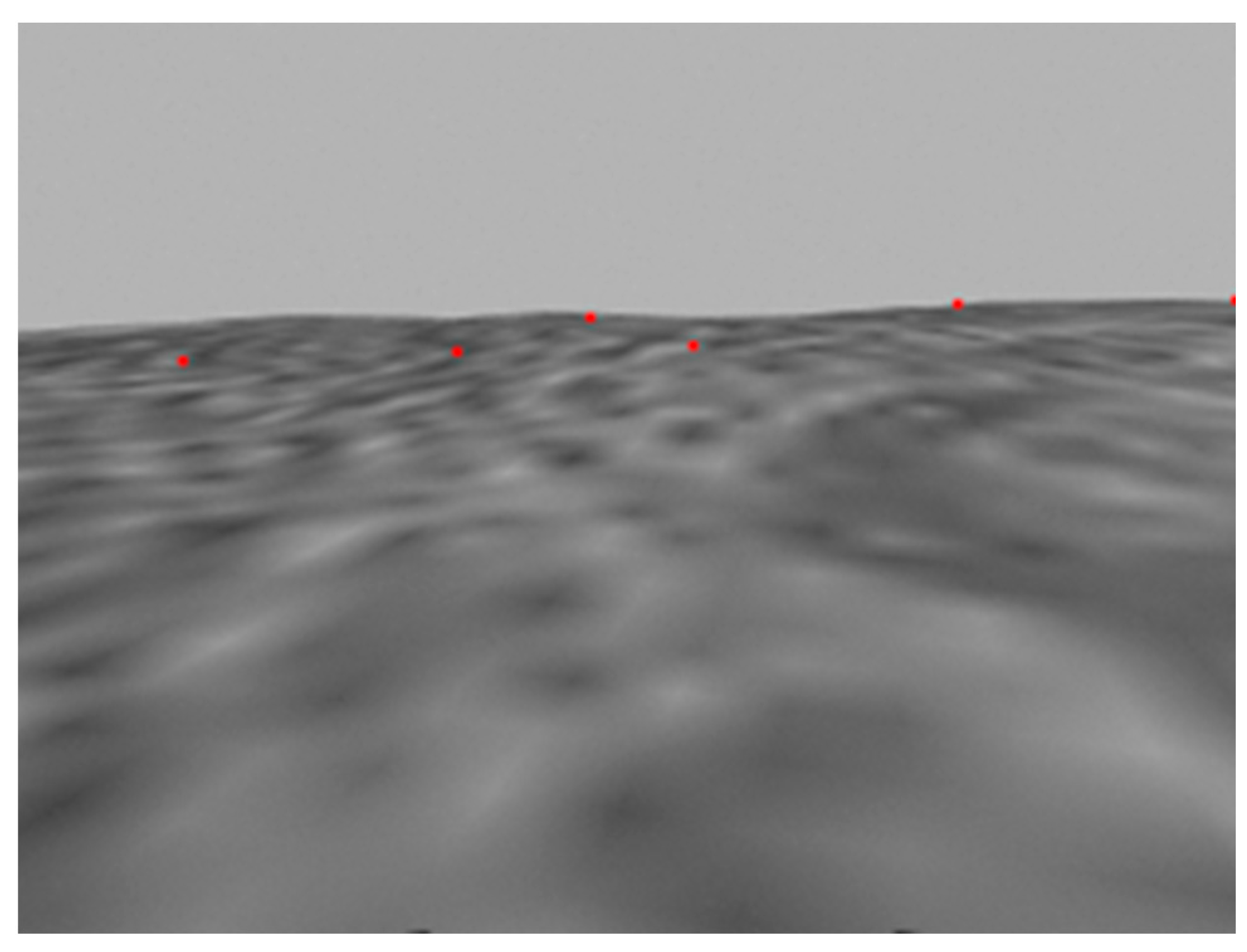
Figure 1. Difficulty in feature extraction (the red dots represent the extracted feature points).
Aerospace 11 00768 g001
Figure 2. Feature matching errors (the lines represent the results of feature matching).
Aerospace 11 00768 g002
Figure 3. The overall framework of the algorithm.
Aerospace 11 00768 g003
Figure 4. Improved SuperPoint visual feature extraction network framework.
Aerospace 11 00768 g004
Figure 5. The process of visual feature tracking.
Aerospace 11 00768 g005
Figure 6. Simulation model construction process.
Aerospace 11 00768 g006
Figure 7. Simulation models: (a) lunar; (b) Mars.
Aerospace 11 00768 g007
Figure 8. Simulated lunar image pair.
Aerospace 11 00768 g008
Figure 9. Simulated Mars image pair.
Aerospace 11 00768 g009
Figure 10. The performance of three feature tracking methods on lunar surface (the lines represent the results of feature matching).
Aerospace 11 00768 g010
Figure 11. The performance of three feature tracking methods on Mars (the lines represent the results of feature matching).
Aerospace 11 00768 g011
Figure 12. Trajectory comparison: (a) Mars; (b) lunar.
Aerospace 11 00768 g012
Figure 13. Trajectory error comparison: (a) Mars; (b) lunar.
Aerospace 11 00768 g013aAerospace 11 00768 g013b
Table 1. Comparison of feature extraction count, mismatch count, and runtime for three visual feature tracking modules (red and bold formatting is used to indicate the best performance).
PlantEvaluation IndicatorsST + LKSP + KNNOurs
LunarExtract feature numbers7425
Correct matching numbers6425
Correct matching rate (%)85.7%100%100%
Mismatch numbers100
Mismatching rate (%)14.3%0%0%
runtime(s)0.0220.3620.292
MarsExtract feature numbers143038
Correct matching numbers83038
Correct matching rate (%)57.1%100%100%
Mismatch numbers600
Mismatching rate (%)42.9%0%0%
runtime(s)0.02718.9780.296
Table 2. Analysis of positioning accuracy of four SLAM algorithms in simulated lunar and Mars environments (red and bold formatting is used to indicate the best performance).
PlantEvaluation IndicatorsLego-LOAMORB-SLAM2LVI-SAMOurs
LunarRmse (m)18.8923.3813.8833.164
Mean (m)17.2812.9533.6172.894
Accuracy Improvement Value (m)///0.723
Percentage increase in accuracy (%)///20%
Marsrmse (m)5.2742.4261.0030.965
mean (m)4.1782.0300.7700.716
Accuracy Improvement Value (m)///0.054
Percentage increase in accuracy (%)///7%
Disclaimer/Publisher’s Note: The statements, opinions and data contained in all publications are solely those of the individual author(s) and contributor(s) and not of MDPI and/or the editor(s). MDPI and/or the editor(s) disclaim responsibility for any injury to people or property resulting from any ideas, methods, instructions or products referred to in the content.