Abstract
This study investigates the application of deep learning models—specifically Deep Neural Networks (DNN), Long Short-Term Memory (LSTM), and Long Short-Term Memory Neural Networks (LSTM-NN)—to predict panel flutter in aerospace structures. The goal is to improve the accuracy and efficiency of predicting aeroelastic behaviors under various flight conditions. Utilizing a supersonic flat plate as the main structure, the research integrates various flight conditions into the aeroelastic equation. The resulting structural vibration data create a large-scale database for training the models. The dataset, divided into training, validation, and test sets, includes input features such as panel aspect ratio, Mach number, air density, and decay rate. The study highlights the importance of selecting appropriate hidden layers, epochs, and neurons to avoid overfitting. While DNN, LSTM, and LSTM-NN all showed improved training with more neurons and layers, excessive numbers beyond a certain point led to diminished accuracy and overfitting. Performance-wise, the LSTM-NN model achieved the highest accuracy in classification tasks, effectively capturing sequential features and enhancing classification precision. Conversely, LSTM excelled in regression tasks, adeptly handling long-term dependencies and complex non-linear relationships, making it ideal for predicting flutter Mach numbers. Despite LSTM’s higher accuracy, it required longer training times due to increased computational complexity, necessitating a balance between accuracy and training duration. The findings demonstrate that deep learning, particularly LSTM-NN, is highly effective in predicting panel flutter, showcasing its potential for broader aerospace engineering applications. By optimizing model architecture and training processes, deep learning models can achieve high accuracy in predicting critical aeroelastic phenomena, contributing to safer and more efficient aerospace designs.
1. Introduction
Panel flutter is a self-excited aeroelastic instability occurring in thin wing panels or fuselage skins, particularly in supersonic environments [1]. This phenomenon, resulting from the interaction of aerodynamic, inertial, and elastic forces, can lead to structural deformation, fatigue, and damage, impacting flight safety. The critical speed at which flutter occurs is known as the panel flutter speed. Technological advances now allow precise calculations and simulations to analyze various flight conditions and determine panel flutter speed. However, aeroelastic analysis requires coupled calculations of structural and aerodynamic forces, which consume a significant amount of computational resources. Recent advancements in Artificial Intelligence (AI), especially machine learning (ML), offer solutions to complex problems such as predicting equipment failures and improving production efficiency. This study employs AI to predict panel flutter speed and analyze convergence and divergence under different flight conditions. We use Deep Neural Networks (DNN), Long Short-Term Memory (LSTM), and LSTM Neural Networks (LSTM-NN) for numerical analysis, comparing their performance to identify the most effective approach.
Accurate prediction of panel flutter is crucial for aircraft safety and performance. Traditional analytical and numerical methods are often computationally intensive and time-consuming. Surrogate modeling, particularly using ML and deep learning (DL), improves prediction efficiency and accuracy. These techniques effectively handle complex aeroelastic phenomena, reducing computational costs while maintaining high accuracy, and are increasingly adopted in aerospace engineering. Sun and Wang [2] explored ANN surrogate modeling for aerodynamic design, highlighting its efficiency and accuracy. They reviewed ANN principles, data treatment, and the configuration setup, covering applications in design, optimization, and network topology. Teimourian et al. [3] demonstrated the effectiveness of ML algorithms for predicting complex aerodynamic phenomena, similar to our DL models for panel flutter prediction. Both studies emphasize the importance of large diverse datasets and comparative algorithm performance for accurate predictions in aerospace. Antimirova et al. [4] provided guidelines for flutter analysis across various flow regimes, improving aeroelastic prediction accuracy and efficiency, though they noted high computing times. Li et al. [5] showed LSTM networks’ effectiveness in enhancing ROMs for transonic aeroelastic analysis, paralleling our approach.
Shubov [6] analyzed flutter using detailed mathematical models, addressing fluid–structure interactions that explain both qualitative and quantitative aspects of flutter. Fung [7] studied simply supported beams under uniform boundary conditions, finding that stable boundary points lead to complex eigenvalues, potential system vibration divergence, and panel flutter. Systematic research on this phenomenon began in the 1950s, with machine learning offering a solution to the extensive numerical calculations traditionally required to determine flutter speed. Dinulović et al. [8] discussed ML applications in predicting flutter in composite material missile fins, emphasizing the cost and time efficiency compared to traditional methods.
Despite advancements, a gap remains in integrating various flight conditions into a comprehensive aeroelastic framework using DL models. Our study addresses this by using DNN, LSTM, and LSTM-NN to predict panel flutter in aerospace structures. By utilizing a supersonic panel and incorporating various flight conditions, we create a large-scale database of structural vibration data for training. Our research highlights the importance of selecting appropriate hidden layers, epochs, and neurons for robust performance, confirming LSTM-NN’s superior accuracy over DNN and LSTM. These findings underscore the DL techniques’ potential in advancing aerospace engineering, offering safer and more efficient aircraft designs. Najafabadi [9] emphasized big data and deep learning in modern data science, noting their importance for analyzing large, raw, and unlabeled datasets across various domains. Hao [10] explained AI development trends, highlighting AI’s growing influence since 2000. Olston et al. [11] discussed TensorFlow, an interface for executing machine learning algorithms on various computer systems. TensorFlow is widely used in fields like speech recognition, computer vision, and natural language processing, making it the ideal choice for building our deep-learning training models.
Traditional methods for predicting panel flutter, such as linear and non-linear analytical techniques, have been well-studied. Foundational theories by Bisplinghoff et al. [12] and Dowell et al. [13] necessitate complex calculations and assumptions. Our DL models, especially LSTM and LSTM-NN, learn directly from large datasets, providing higher accuracy and robustness across diverse flight conditions. Numerical simulations using Computation Fluid Dynamics (CFD) and Finite Element Method (FEM) offer detailed insights but are computationally intensive (Sayed et al. [14] and Lamorte and Friedmann [15]). Our DL models provide significant computational advantages by quickly predicting panel flutter once trained, which is beneficial for design optimization and real-time monitoring. This speed advantage is particularly beneficial in design optimization and real-time monitoring applications.
Deep learning models, such as LSTM and LSTM-NN, capture complex non-linear relationships and long-term dependencies in the data, leading to more accurate and reliable predictions. DL models are highly scalable and can be trained on extensive datasets. This scalability ensures that our models are robust and generalize well to various flight conditions and panel configurations. Deep learning, a subset of machine learning (ML), is based on AI architecture. The “depth” in deep learning refers to the multiple layers in neural networks. In 2006, Hinton et al. [16] introduced a fast-learning algorithm for deep neural networks utilizing three hidden layers, significantly improving accuracy but occasionally resulting in overfitting. To address this, Hinton [17] proposed the Dropout method to prevent overfitting. In 2014, Kingma and Ba [18] introduced the Adam optimizer, combining AdaGrad and RMSProp benefits for handling sparse gradients and unstable objectives, offering easy implementation and low memory requirements, and demonstrating convergence speed and stability.
In the 1950s, Rosenblatt [19] introduced the perceptron model, which only solved linear problems. Later, Werbos [20] proposed backpropagation, providing a critical method for neural network training. Hopfield [21] introduced Hopfield networks in 1982 for associative memory and optimization problems. In 1997, Hochreiter and Schmidhuber [22] proposed Long Short-Term Memory (LSTM), addressing issues in recurrent neural networks (RNN), particularly the vanishing gradient problem, improving training speed and solving long-term dependencies. Ding et al. [23] discussed activation functions’ importance in deep learning models, emphasizing the role of non-linear elements in enhancing neural network performance. Keskar et al. [24] noted that large-batch methods in stochastic gradient descent (SGD) reduce generalization due to noise in gradient estimation, while small-batch methods tend to achieve flatter minima. Solgi et al. [25] used LSTM-NN for groundwater level prediction, demonstrating its superior accuracy over simple neural networks for long-term and short-term predictions, even for extreme events. Liao et al. [26] proposed a machine learning strategy for preliminary bridge design, showing that ML models offer superior prediction capabilities, verifying their applicability in aeroelastic mechanics. Sabater et al. [27] used DL to predict aircraft surface pressure distribution, finding that deep neural networks outperformed other methods, providing a new approach for design and optimization in aviation. Baykal et al. [28] utilized TensorFlow for DL systems, classifying images using the MNIST dataset, showing significant GPU performance improvements. Buber and Banu [29] conducted performance analysis tests on DL, emphasizing hyperparameters affecting performance and demonstrating GPU’s superior execution speed over CPU, highlighting that increasing core numbers and batch sizes enhances parallel processing capability.
In this paper, we investigate how varying the aspect ratio of a small panel within an aircraft skin structure affects structural flutter under different flight altitudes, speeds, and environmental conditions. We categorize and analyze various scenarios to evaluate flutter speed and stability. Using supervised machine learning, we divide data into training, validation, and prediction sets to identify the most efficient algorithm. We predict panel flutter with the three following algorithms: Deep Neural Network (DNN), Long Short-Term Memory (LSTM), and Long Short-Term Memory Neural Network (LSTM-NN). Our study demonstrates that LSTM-NN is more accurate than DNN and LSTM in predicting panel flutter, thanks to its ability to capture long-term dependencies and sequential patterns. These findings highlight the potential of deep learning techniques in advancing aerospace engineering, offering pathways to safer and more efficient aircraft designs.
2. Theoretical Analysis of Aeroelasticity
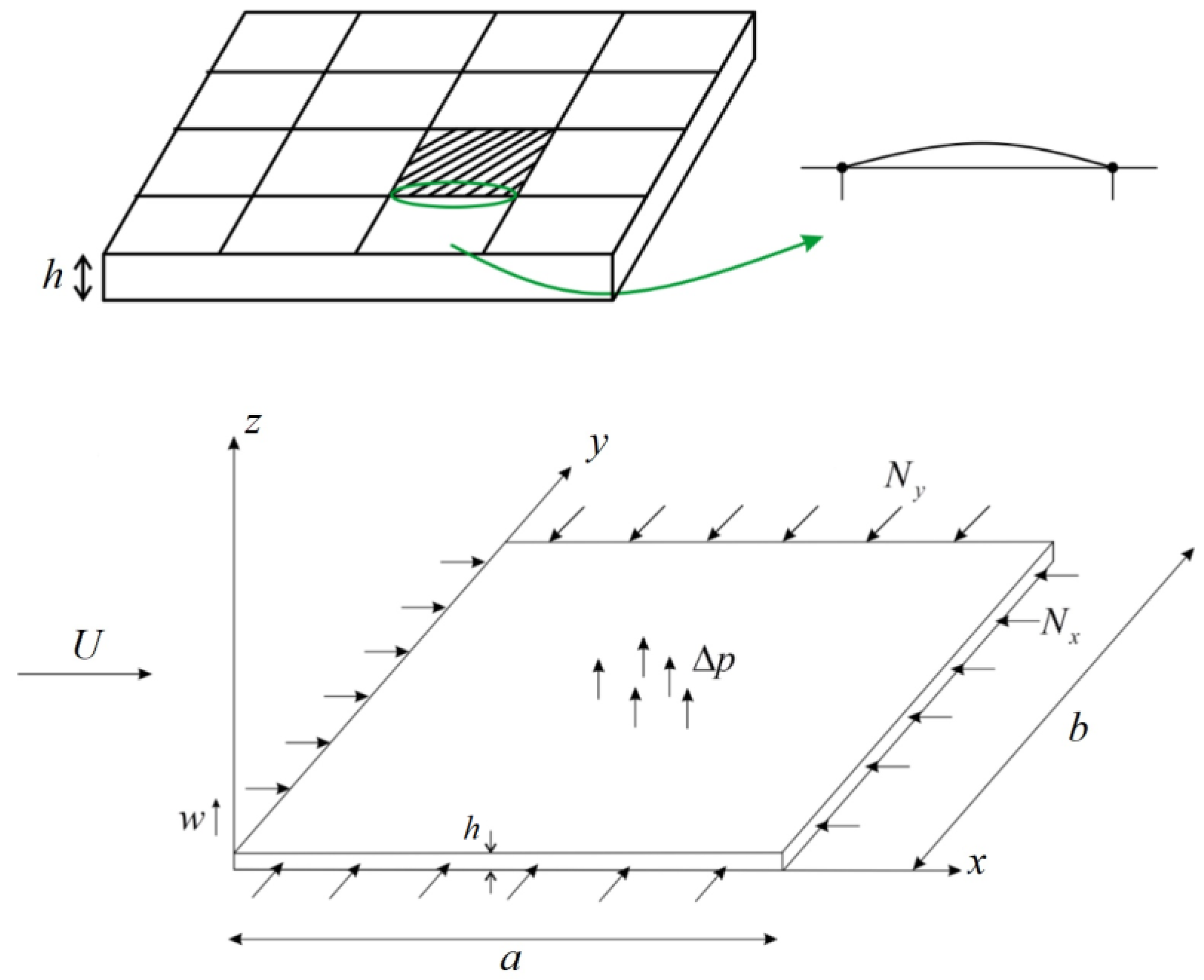
Panel flutter is an aeroelastic phenomenon in aircraft, characterized by oscillations resulting from the coupling of aerodynamic forces, elasticity, and inertia. These vibrations usually have large amplitudes, which can easily lead to elastic fatigue and damage to the structure. This phenomenon is more likely to occur in parts like the wings, fuselage, and the tail of an aircraft. Therefore, at any flight speed and altitude, aeroelastic calculations are necessary [30]. As shown in Figure 1, the small panel is subjected to pressures Nx and Ny around its edges, with a relative wind speed of U. The length of the panel is denoted by a, the width by b, and w represents the amplitude in the z-direction.
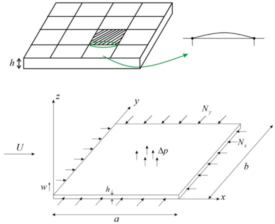
Figure 1.
Illustration of panel flutter.
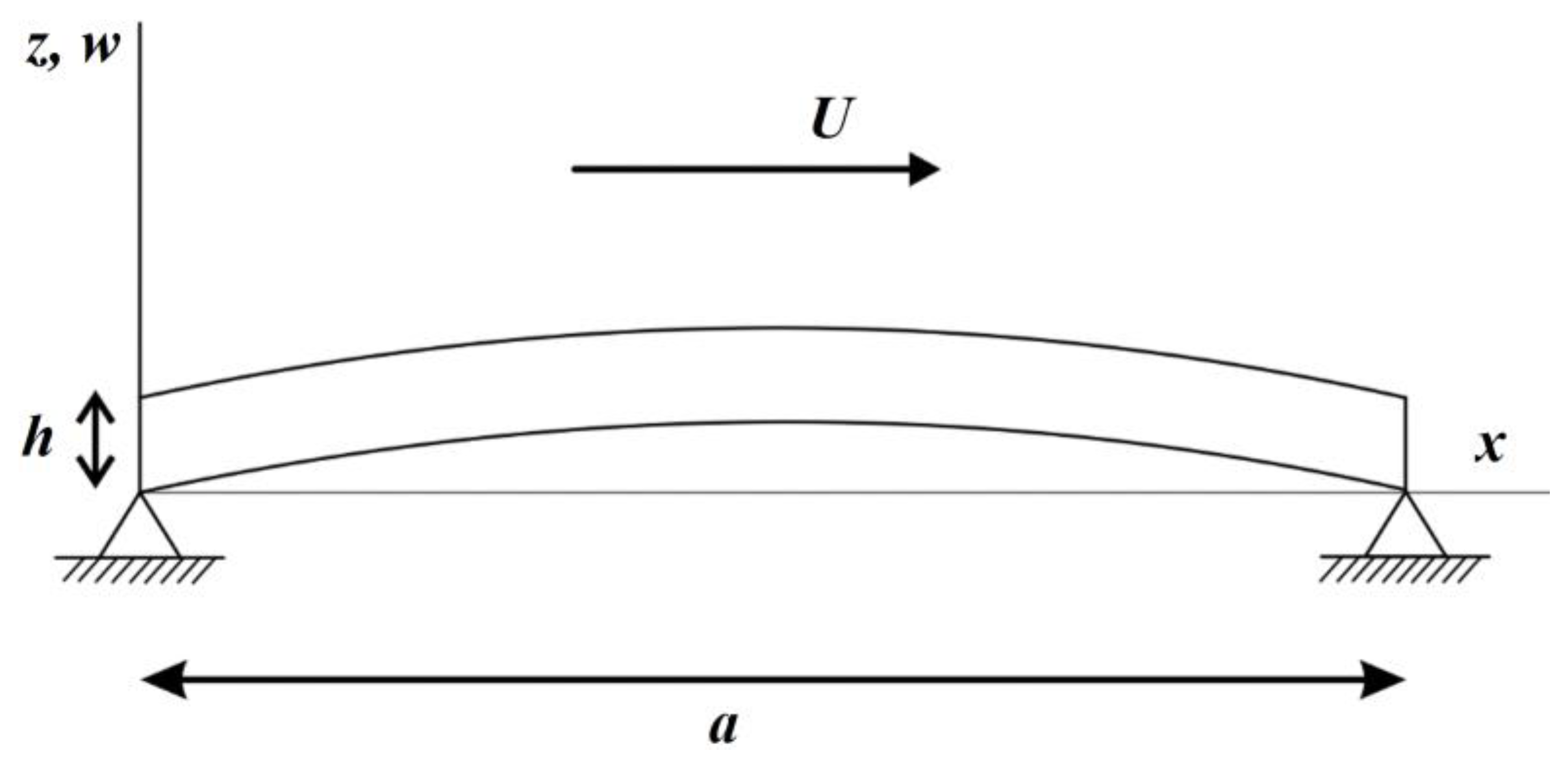
Consider a small panel with an external flow velocity of U, as illustrated in Figure 2. The conditions for panel flutter are constrained to supersonic speeds. Mathematically, the plate equation can be expressed through the principles of Hookean material elasticity and the equations of structural dynamics, as follows:
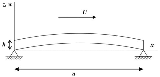
Figure 2.
External flow field of a panel.
In which represents the density of the panel’s material, h represents the panel’s thickness, represents the air pressure, represents the structural damping term, and D represents the stiffness of the panel and can be written as . Additionally, E is the Young’s modulus and is the Poisson’s ratio. For supersonic Mach numbers, the pressure can be approximated using first-order piston theory with the function as follows:
where M represents the Mach number. To calculate the panel flutter of a rectangular plate, we assume that it is simply supported and the boundary conditions are as follows:
Let the dimensionless parameters be , , and . We use w to represent the displacement in the z-direction for ease of analysis. After simplification, Equation (1) can be expressed as
gT is the total damping coefficient of the system, is the dimensionless structural damping, ga is the air damping coefficient, is the air density, and represents the dimensionless load in the x and y directions, which can be expressed as
Here, Nx is the load in the x direction and Ny is the load in the y direction. Using the method of separation of variables, let
Equation (7) can be rewritten as
The time domain equation can be expressed as
Assuming the time–domain function T of the small panel can be expressed as , where , is the decay rate, and is the nondimensional frequency. The boundary conditions of the small panel are . Assuming the wind pressure acting on the small panel in the x direction is much greater than that in the y direction, in Equation (10) can be expressed as
Substituting Equation (13) into Equation (11) yields
where
By substituting the parameters into Equations (15)–(17), we can express the general solution for the vibration of the small panel as
where z1~z4 are the four roots of the complex characteristic equation (Equation (14)). These roots satisfy the following determinant:
This determinant (Equation (19)) represents the condition for the existence of a non-trivial solution for the vibration problem, ensuring that the panel exhibits the specified flutter characteristics. Expanding the determinant of Equation (19) yields a complex solution. The real part of this solution is used to determine whether the panel flutter converges, diverges, or reaches a stability boundary. If Ik < 0, the oscillation converges; if Ik = 0, it is at the stability boundary; and if Ik > 0, the oscillation diverges. The data are divided into three categories for training and prediction. First, we substitute various flight conditions into Equation (14), perform the calculations, and then substitute the results into Equation (19) to obtain a complex solution. Based on the value of the real part, flight conditions are classified into three types: if the real part is 0, it is a stability boundary, marked as “1”; if the real part is less than 0, it is a stable state (converge), marked as “2”; and if the real part is greater than 0, it is an unstable state (diverge), marked as “0”. The predicted flutter speed uses the Mach number corresponding to a real part of 0 as the label for prediction. The flight condition parameters we collected include the aspect ratio (a/b), Mach number (M), flight altitude, and the values of and in the time–domain function (T). Table 1 shows the parameters used for data collection. We collected a total of 707,472,000 data points and 197,621 data points were obtained for the flutter speed (Mach number) prediction at the stability boundary. The design space of our study is defined by four key parameters: the panel aspect ratio, Mach number, air density, and decay rate. To ensure comprehensive coverage of the design space and to capture the complex interactions between these parameters, a large dataset is necessary. A large number of samples ensures that we capture the detailed variability and the full range of possible interactions between the four parameters. This comprehensive sampling is crucial for training robust deep-learning models that generalize well to unseen data. With more data, our models can learn more nuanced patterns and dependencies, leading to improved prediction accuracy. This is particularly important in aeroelastic applications where accurate predictions are critical for safety and performance. A larger dataset also helps in mitigating overfitting by providing sufficient data for training, validation, and testing. This ensures that the models do not simply memorize the training data but learn to generalize from it. To select the samples, we employed a systematic approach rather than a purely random one. We divided the range of each parameter into very small intervals (0.001). This fine-grained division ensures that the dataset adequately covers the entire design space and captures even the smallest variations and interactions between parameters. This approach ultimately enhances the models’ generalizability and performance in predicting panel flutter under various flight conditions.

Table 1.
Parameters and labels used in the aeroelastic equations.
Traditional methods for predicting panel flutter in aerospace structures often rely on extensive Computational Fluid Dynamics (CFD) simulations and wind tunnel tests, which are both time-consuming and resource-intensive. These methods typically require a significantly smaller number of data points compared to machine learning approaches. To put this into perspective, traditional CFD simulations might use around 10,000 to 100,000 data points for a detailed analysis of panel flutter. This range allows for capturing the essential aerodynamic and structural interactions without the need for an excessively large dataset. However, these simulations must be repeated for various conditions (e.g., different Mach numbers, aspect ratios, and flight altitudes) to cover a comprehensive range of scenarios, which cumulatively increases the data requirements. In contrast, machine learning models, especially deep learning, require large datasets to learn the complex relationships and patterns within the data effectively. Our dataset of 707,472,000 data points includes a wide range of flight conditions and structural parameters, providing a robust basis for training and validating our deep learning models. Additionally, the large dataset enables our models to generalize better across different scenarios, reducing the reliance on repeated simulations for each new condition. By leveraging this extensive dataset, we aim to develop models that can predict panel flutter with high accuracy and efficiency, ultimately reducing the need for extensive traditional simulations. We acknowledge that the method provided in this study is indeed trained on a simplified aeroelastic equation, which inherently carries the same limitations as the classical flutter analysis it is based on. This was a deliberate choice, driven by the specific objectives of our research. The primary goal of our study was to explore the feasibility and effectiveness of DL techniques in predicting panel flutter using a well-established and widely validated classical equation. While this classical flutter analysis does not achieve the same level of accuracy as more sophisticated CFD-FEM coupled systems, it offers a solid foundation for an initial exploration into the application of AI in aeroelasticity. By working within a controlled and well-understood framework, we were able to validate our DL models and demonstrate their potential in efficiently predicting panel flutter in a computationally less expensive manner.
3. Deep Learning
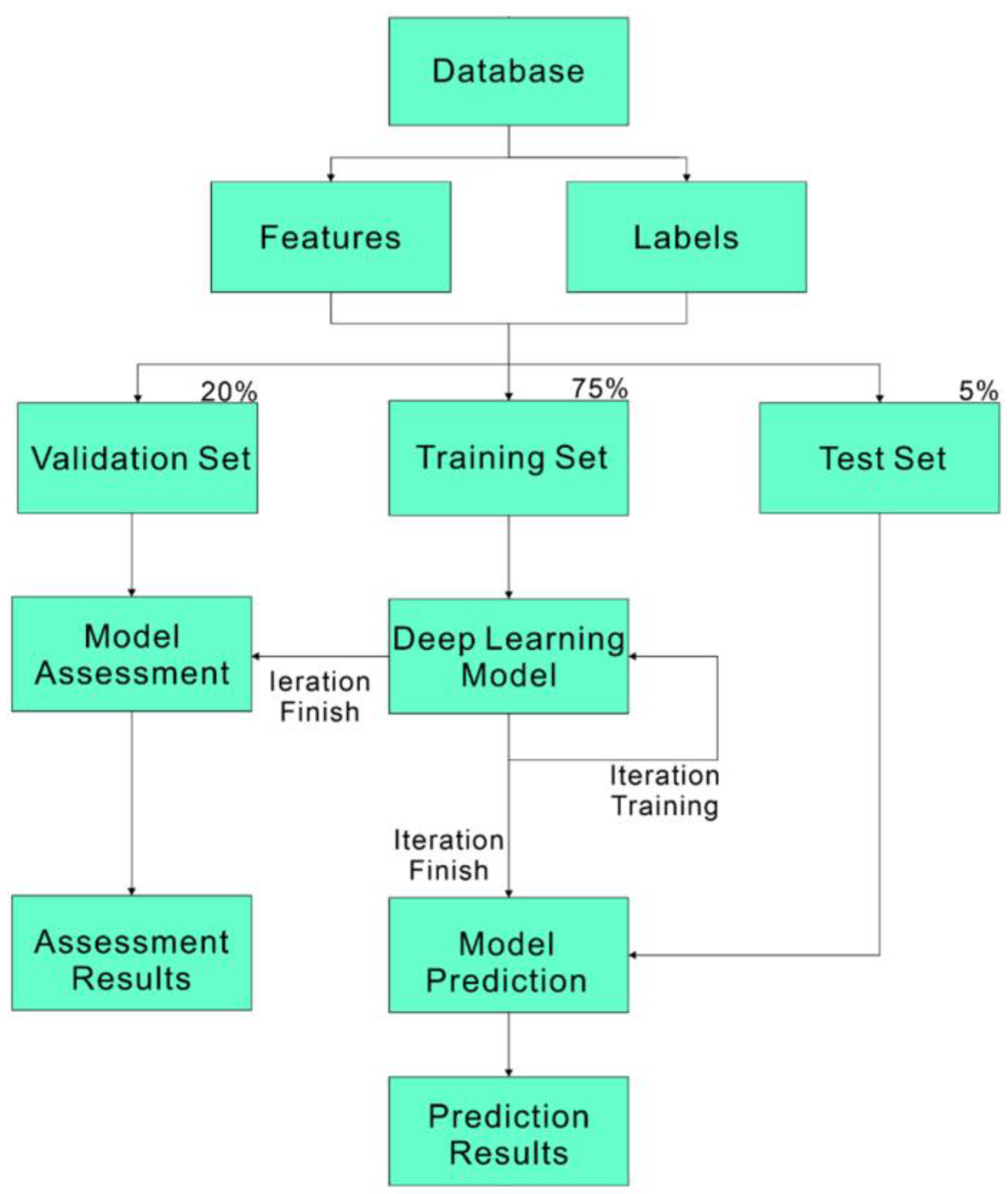
Deep learning is a branch of Machine Learning (ML) within the broader field of Artificial Intelligence (AI) [31]. Machine learning is a powerful technique that analyzes and recognizes large datasets, emulating the way the human brain processes information to accomplish various tasks and solve problems. We will use machine learning algorithms to predict the convergence of panel flutter and the supersonic flutter speed or Mach number, as well as to analyze their physical significance. Deep learning imitates the functioning of the human brain [32], utilizing multi-layer neural networks to learn features and patterns from data. These networks are composed of an input layer, hidden layers, and an output layer. The architecture simulates the connections between neurons in the human brain, with each layer performing different operations on the data. Unlike traditional shallow learning, which requires manual design and feature extraction from data, deep learning automatically learns features by increasing the number of hidden layers, thus more effectively handling complex problems. Although shallow learning models may train faster, they cannot match the performance of deep learning on complex datasets. Therefore, we chose deep learning to build our model. We divided the data into three parts: training set, validation set, and prediction set. First, the training data are fed into the neural network, where neurons in multiple hidden layers perform calculations. These calculations are repeated until the predictions accurately match the correct feature values. A loss function is used to measure the model’s prediction accuracy, aiming to minimize the loss function. Finally, the prediction set is used to evaluate the model’s performance. The prediction set is input into the trained model to obtain prediction results, as illustrated in Figure 3.
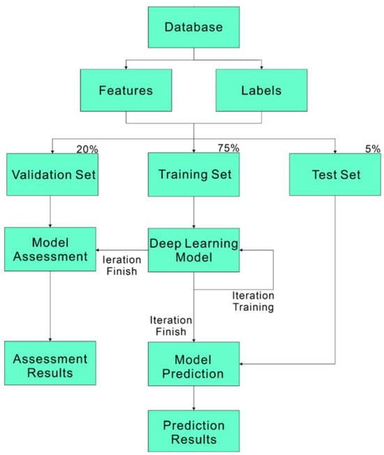
Figure 3.
Deep learning flowchart.
3.1. Deep Neural Networks Architecture
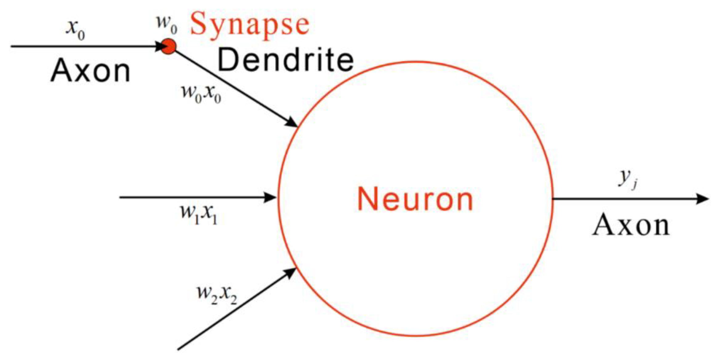
Deep Neural Networks (DNN) consist of multiple layers of interconnected neurons, where each neuron receives activations from the previous layer as inputs and performs computations. Figure 4 illustrates the structure of an artificial neuron and Equation (20) represents the mathematical formulation of a neuron.
where y is the output of the neuron, f is the activation function, wi are the weights, xi are the inputs, and b is the bias term. The process involves forward propagation, where inputs pass through the layers to produce an output, and backpropagation, where errors are propagated back to adjust the weights and biases, optimizing the network’s performance. This architecture allows DNNs to learn intricate patterns and representations from the data, making them suitable for tasks such as image recognition, natural language processing, and in our case, predicting the flutter phenomenon in small panels under various flight conditions.

Figure 4.
Diagram of an artificial neuron.
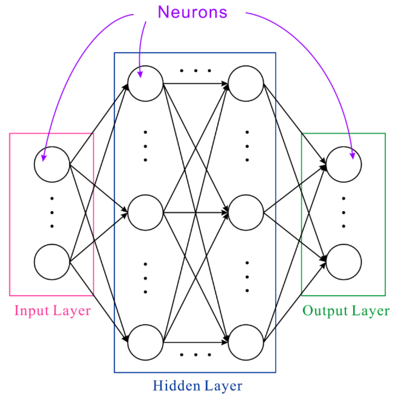
Deep learning often references Brain-Inspired Computation, which refers to algorithms or programs that mimic basic patterns of human brain operation. In neurons, signals pass through axons, synapses, and dendrites, where dendrites receive input signals, compute them, and generate an output signal along the axon. These inputs and outputs are termed activations. Synapses convey signals (xi) from input values, each with a weight (wi). By multiplying all input values by their respective weights and passing them through an activation function, a new output value (yi) is generated, as expressed in Equation (20). During this process, i input weights plus one bias value (b) is necessary, all of which must be trained in order to acquire prior knowledge or labeled training data. The use of an activation function is essential because, following activation, neurons can learn non-linear data relationships. The structure of a deep neural network primarily includes three architectures: an input layer, a hidden layer, and an output layer. Neurons in the input layer accept data and send it on to neurons in the network; this layer is frequently referred to as the hidden layer. Weighted output from numerous hidden layers is transferred to the output layer, a process shown in Figure 5.
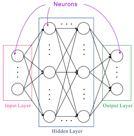
Figure 5.
Deep neural network architecture diagram.
3.1.1. Objective Function of Deep Neural Networks
In machine learning, most algorithms aim to maximize or minimize a specific function or metric known as the Objective Function. The Loss Function is a component of the objective function used to measure the error between the model’s predictions and the actual values. Commonly used loss functions include Categorical Cross-Entropy and Mean Squared Error (MSE). In this study, for training under three flight conditions, we utilize Categorical Cross-Entropy, which is typically applied in classification tasks. This method measures the discrepancy between the model’s predicted output probability distribution and the true value’s probability distribution. The formula for Categorical Cross-Entropy is given by
Here, c represents the number of classes, yi denotes the true probability distribution, and indicates the model’s predicted probability distribution.
3.1.2. Back Propagation Algorithm
The Back Propagation Algorithm is centered on the concept of propagating error values from the output layer to the input layer. This enables the weights in the neural network to undergo gradient descent based on these error values, gradually reducing the network’s overall error. The Back Propagation Algorithm leverages the Chain Rule from calculus to compute and store gradient information across each layer of the neural network, based on the difference between the network’s output and the true output. Through iterative training and adjustment, the algorithm stabilizes the weights to enhance network performance. The gradients of the loss function across each neural network layer are computed as shown in Equation (22). Once these gradients are obtained, they are used to update the weights, continuously improving the neural network’s ability to match its targets effectively.
This process iteratively enhances the neural network’s performance by iteratively computing the difference between the neural network’s output values and the target values.
3.2. Basic Architecture of Long Short-Term Memory (LSTM)
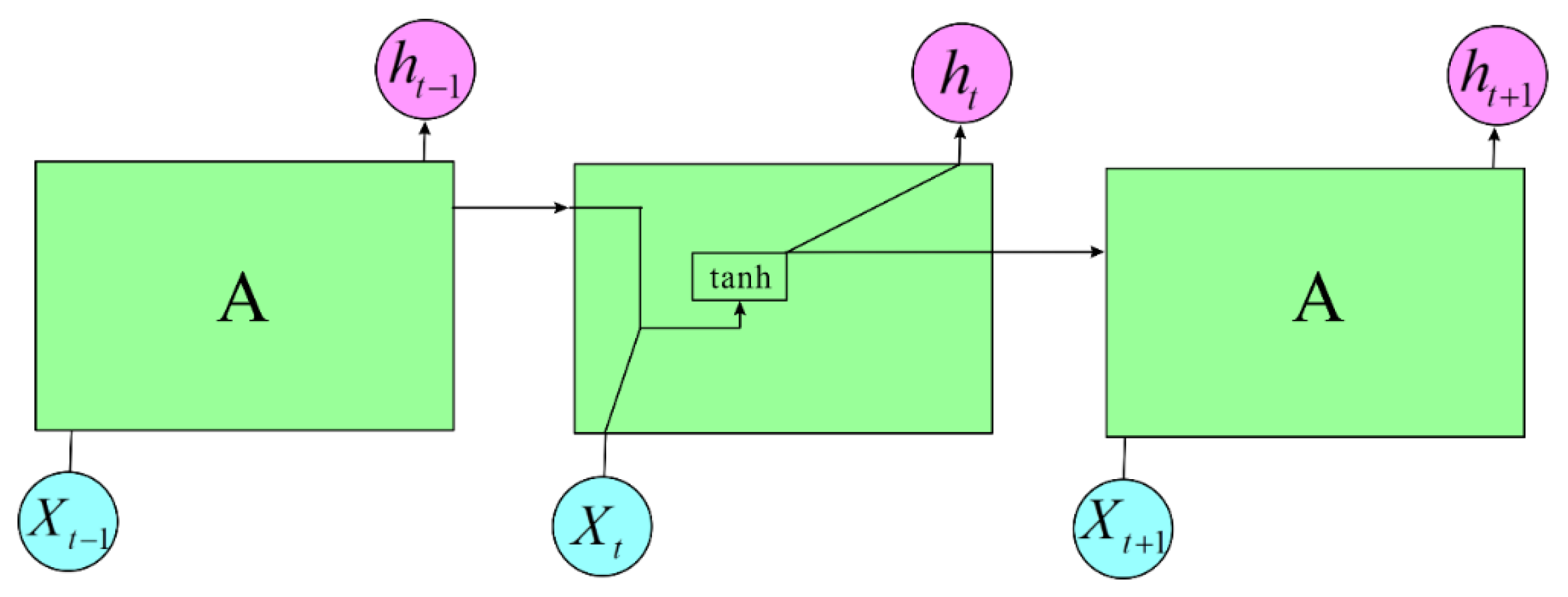
Long Short-Term Memory (LSTM) is a specialized type of Recurrent Neural Network (RNN) designed to address the challenges of training on long sequences, specifically mitigating the vanishing gradient and exploding gradient problems. In standard RNNs, the vanishing gradient problem arises due to the use of activation functions like the tanh function. During backpropagation, gradients are propagated back through time, and if the initial gradients are less than 1, repeated multiplication by tanh activations can cause gradients to diminish exponentially, resulting in vanishing gradients. Conversely, if the initial gradients are sufficiently large, they can cause subsequent gradients to explode exponentially. LSTM addresses these issues through its unique architecture, which includes gating mechanisms (input, forget, and output gates) that regulate the flow of information through the cell. This helps preserve long-term dependencies and mitigate the issues of vanishing or exploding gradients commonly encountered in traditional RNNs. Figure 6 is a simplified illustration of a basic RNN model, as follows:
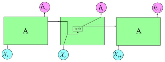
Figure 6.
RNN model.
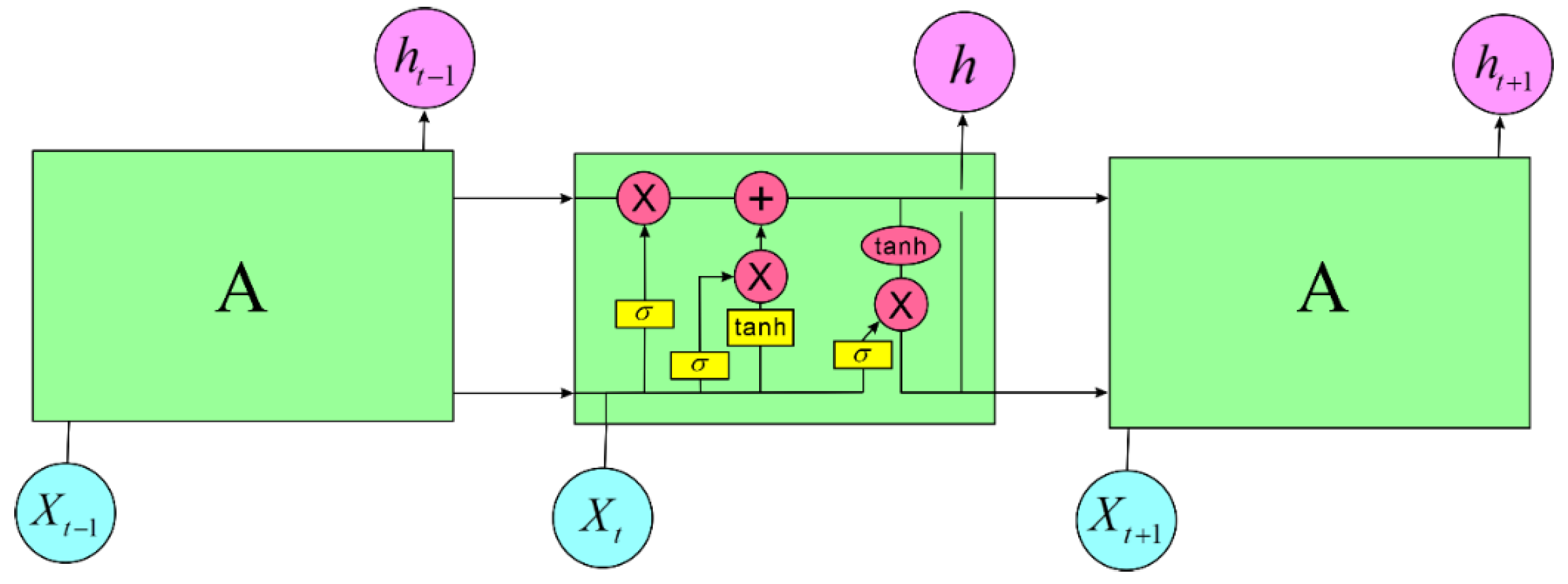
LSTM (Long Short-Term Memory) differs from traditional RNNs primarily in its computational process. While standard RNNs consist of a single neural network layer that processes sequential data, LSTM introduces a more complex architecture with four interacting neural network layers arranged in a very specific way. This architecture allows LSTM to effectively address the challenges of learning long-term dependencies, which are problematic for vanilla RNNs due to issues like vanishing and exploding gradients. The LSTM model is depicted as shown in Figure 7.
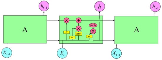
Figure 7.
LSTM model.
In LSTM, the first step involves using a mechanism called the Forget Gate to determine which information to retain in the cell state and which to discard. This process is handled by the Forget Gate, which considers the previous time step’s output ht−1 and the current time step’s input Xt to output a value between 0 and 1 for each number in the cell state Ct−1. A value close to 1 indicates that the corresponding information should be retained, while a value closer to 0 indicates that the information should be discarded the h.
3.2.1. Objective Function of Long Short-Term Memory (LSTM)
Long Short-Term Memory (LSTM) models also require an objective function for evaluation. Mean Square Error (MSE) is a commonly used objective function for regression problems, measuring the difference between model predictions and actual values. It is computed by squaring the difference between the model’s prediction and the actual value yi, for each sample, and then averaging these squared differences across all samples. The MSE for a model trained on n training data points is expressed as Equation (23), as follows:
3.2.2. Backpropagation through Time (BPTT) in LSTM
LSTM integrates Backpropagation Through Time (BPTT), which is crucial for handling time series data in deep learning. Through the BPTT training process, LSTM minimizes the model’s loss function by adjusting weights and biases based on the difference between actual outputs and expected outputs, thereby enhancing model performance.
3.2.3. Training Parameter Configuration
The optimizer plays a critical role in training neural networks in deep learning. It adjusts the weights and errors in the neural network to minimize the model’s loss function, gradually updating model parameters through iterative processes to converge to an optimal state. We chose to use the Adam optimizer introduced by Kingma and Ba [18]. Adam combines the Adagrad and Momentum algorithms. Adagrad is an adaptive learning optimization algorithm that adjusts the learning rate based on historical gradient information for each parameter. Parameters with larger gradients have smaller learning rates, while those with smaller gradients have larger learning rates. Equation (24) represents the equation for Adagrad:
Here, wi+1 is the updated parameter at time step i + 1, is the learning rate, Gi,i is the accumulated sum of the squared historical gradients for the parameter wi, J is the gradient at time step i, and is a small constant to prevent division by zero.
Momentum is an optimization algorithm based on momentum. The formulas for Momentum are given in Equations (25) and (26).
represents the gradient of the loss function with respect to the parameter wi, vi is the momentum of the parameter wi, and is the momentum coefficient, which indicates the relationship between the momentum and the gradient update weights. The core idea of Momentum is to accumulate previous gradient information during each update and adjust the parameters based on this information. Momentum endows gradient updates with a certain inertia, helping to accelerate convergence.
Adam is an optimization algorithm that combines Adagrad and Momentum, assigning different weights to different gradients. Initially, the first moment m0 and the second moment v0 of the gradient are both assumed to be zero, with bias correction coefficients and also set to zero. For a small batch Bt at time step t, the gradient gt is calculated and the exponentially weighted moving averages of the first and second moments of the gradients are updated. The formulas are given in Equations (27) and (28).
The bias-corrected gradient as well as is shown in Equation (29).
Here, and represent and raised to the power of t, respectively. The updated weights are given by Equation (30).
Here, is the learning rate and is a constant added to enhance stability. In the program, the parameters are set as = 0.0003, = 0.9, = 0.999, and = 10−8.
In deep learning, activation functions introduce non-linearity, allowing neural networks to learn complex non-linear relationships and mitigating the vanishing gradient problem. The activation functions used in our model training include Rectified Linear Unit (ReLU), Softmax Function, and Hyperbolic Tangent Function. The ReLU function has a derivative, allows for backpropagation, and can improve computational efficiency. When the input is less than zero, the output is zero; when the input is greater than zero, the output equals the input, exhibiting a linear growth characteristic. Equation (31) illustrates the definition of the ReLU function.
The Sigmoid function produces output values that approach 1 as the input increases and approach 0 as the input decreases. Since probabilities are within the range of 0 to 1, the Sigmoid activation function is typically used in models that output probabilities. Equation (32) depicts the Sigmoid function.
The Softmax function converts input values into real numbers between 0 and 1, typically used in the final layer of a neural network. The Softmax operation ensures that the sum of the output probabilities equals 1. Equation (33) illustrates the Softmax function.
The Tanh function ranges between −1 and 1, making it easier to handle large positive and negative values. This helps to center the data, facilitating learning in subsequent layers. Equation (34) illustrates the definition of the Tanh function.
3.3. Evaluation Metrics for Machine Learning Performance
Evaluating the performance of a machine learning model is crucial to determining its effectiveness and reliability. This study will use four common metrics: Confusion Matrix, Mean-Square Error (MSE), Coefficient of Determination (R-squared), and Relative Error to assess the model’s fit and predictive capabilities.
The Confusion Matrix is one method used to evaluate the performance of classification models, especially suitable for supervised learning. Its advantage lies in visualizing the data; each column of the matrix represents the actual predictions of a category, showing the number of times the model correctly and incorrectly classified samples, which are then converted into percentages.
MSE (Mean-Square Error) is a method most commonly used for regression loss functions. It calculates the average of the squares of the differences between the predicted and actual values. The lower the MSE, the more accurate the model’s predictions. However, MSE is very sensitive to extreme values, which can significantly impact the result due to a single outlier.
R-squared is another commonly used performance metric derived from residuals. It measures the extent to which the model explains the variance in the dependent variable. The R-squared value ranges from 0 to 1, with values closer to 1 indicating a stronger understanding of the data by the model and values closer to 0 indicating a weaker understanding. For a dataset with n data points and corresponding predicted values f1, …, fn, the residual is defined as ei = yi − fi and the mean is . Subsequently, we can derive the total sum of squares, , and the residual sum of squares, . Then, R-squared can be defined as .
Relative Error is another metric for evaluating the accuracy of predictions and is one of the most encountered in common. It helps us understand the degree to which a model fits the actual values. A lower relative error indicates more accurate predictions by the model. This metric is often used to assess the performance of predictions for continuous variables, such as in regression problems. It provides insight into the model’s predictive ability across different scenarios and aids in adjusting and improving the model.
4. Deep Learning Training Analysis and Results
Based on the aeroelastic equations of motion for airfoil discussed in Section 2 and the deep neural network architecture referenced by Montavon and Samek [33], we have constructed a deep neural network capable of predicting divergence, convergence, stability boundaries, and flutter speed of small panels. Various parameters and data optimizations were applied to build this predictive model. Finally, we analyzed the impact of these parameters on the physical significance of the predictions through graphical representation.
4.1. Comparison of Different Hardware
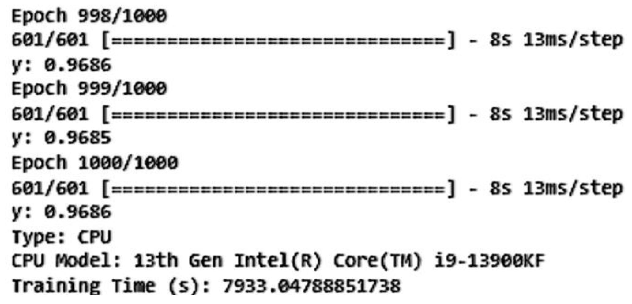
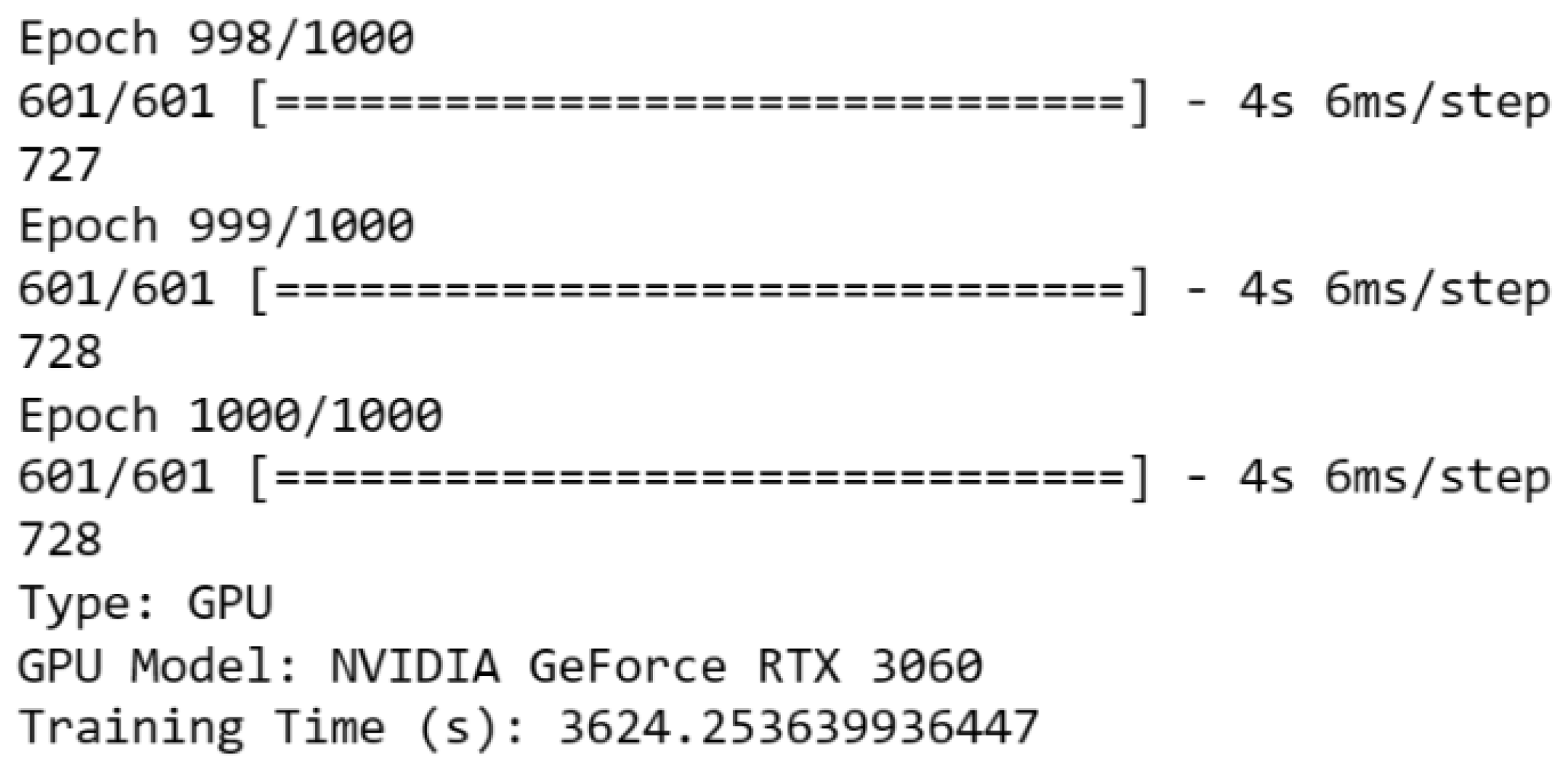
Before training the model, we compared the training speed of machine learning models on a CPU and a GPU and examined the impact of different GPU models on training time. We utilized an Intel Core i9-13900KF processor (Designed by Intel®, manufactured by TSMC, Hsinchu, Taiwan) and an NVIDIA GeForce RTX 3060 GPU (Manufactured by Micro-Star International Co., Ltd., New Taipei City, Taiwan), using the TensorFlow framework for testing. We trained the same machine-learning model on both the CPU and GPU and recorded the training time. The epoch and total training time on CPU and RTX 3060 GPU are shown in Figure 8 and Figure 9, respectively. The results indicate that training on the GPU is significantly faster than on the CPU. We tested with one LSTM layer and one NN hidden layer, with each containing 10 neurons. The training time with the GPU was approximately 50% shorter than with the CPU, demonstrating the significant advantage of using a GPU for training machine learning models.
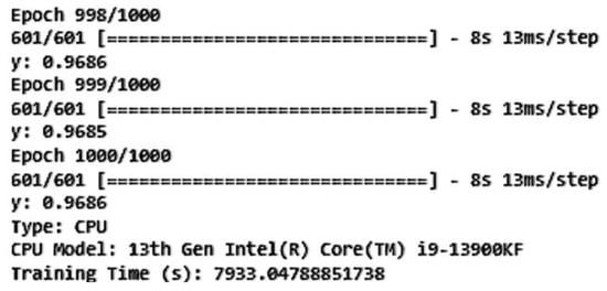
Figure 8.
Epoch and total training time on CPU.

Figure 9.
Epoch and total training time on RTX3060.
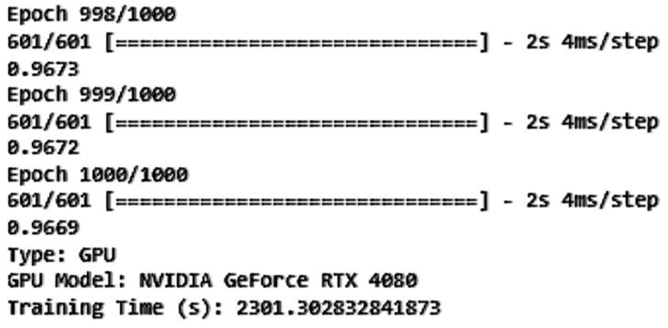
We further examined the impact of different GPUs on training time by using the GeForce RTX 4070 and GeForce RTX 4080 (Manufactured by Micro-Star International Co., Ltd., New Taipei City, Taiwan). By comparing the training times of different GPUs (Figure 10 and Figure 11), we observed significant performance differences between the models. The GeForce RTX 4070 reduced training time by approximately 23% compared to the GeForce RTX 3060 and the GeForce RTX 4080 reduced training time by about 36% compared to the GeForce RTX 4070. Compared to the CPU, the GeForce RTX 4080 shortened training time by about 71%. These results indicate that the configuration and computational power of the GPU have a significant impact on training time.
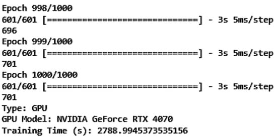
Figure 10.
Epoch and total training time on RTX4070.
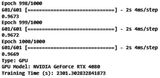
Figure 11.
Epoch and total training time on RTX4080.
This section highlights the hardware comparison and the observed differences in training times with various GPUs. The next steps involve detailing the actual training process, presenting the results, and discussing the implications of these findings in the context of aeroelasticity and flutter prediction.
4.2. DNN Model Construction and Analysis (Divergence, Convergence, and Stability Boundaries)
Using the linear aeroelastic equations of motion for three-dimensional airfoils from Section 2, we established a database with a total of 707,472,000 samples. Training on the entirety of this data would overwhelm the hardware, leading to memory issues and excessively long training times. Please see Figure 12 for the message of memory error.

Figure 12.
GPU memory error.
To manage the data volume, we categorized the data into three different flight outcomes: 0 for divergence, 1 for stability boundary, and 2 for convergence. The sampled data were divided into a 70% training set, a 25% validation set, and the remaining 5% as a test set. Our study utilized a significantly large dataset, consisting of 707,472,000 data points. Given the substantial size of the dataset, even a smaller percentage can represent a large absolute number of data points. In our case, 5% of the dataset equates to approximately 35,373,600 data points. This is a sufficiently large sample to ensure the testing set is representative of the overall data distribution and provides a reliable measure of model performance. The choice of 5% was made with the consideration that it provides an adequate representation of the data’s variability, covering various flight conditions, panel configurations, and other factors relevant to aeroelastic behavior. This ensures that the test set encompasses a broad spectrum of scenarios that the model may encounter. Training and evaluating deep learning models, particularly those with complex architectures like LSTM-NN, on such a large dataset demands significant computational resources and time. By using 5% of the data for testing, we balanced the need for a representative test set with the practical considerations of computational efficiency and resource utilization. A smaller test set size allowed for quicker evaluation cycles, enabling more frequent and timely feedback on model performance. This facilitated iterative improvements to the model and more efficient use of computational resources without compromising the robustness of the evaluation. The primary focus of our study was to investigate the efficacy of deep learning models in predicting panel flutter, rather than the exhaustive evaluation of every possible test set size. By using a 5% test set, we ensured that the core research objectives were met while maintaining computational efficiency and timely feedback for model improvements.
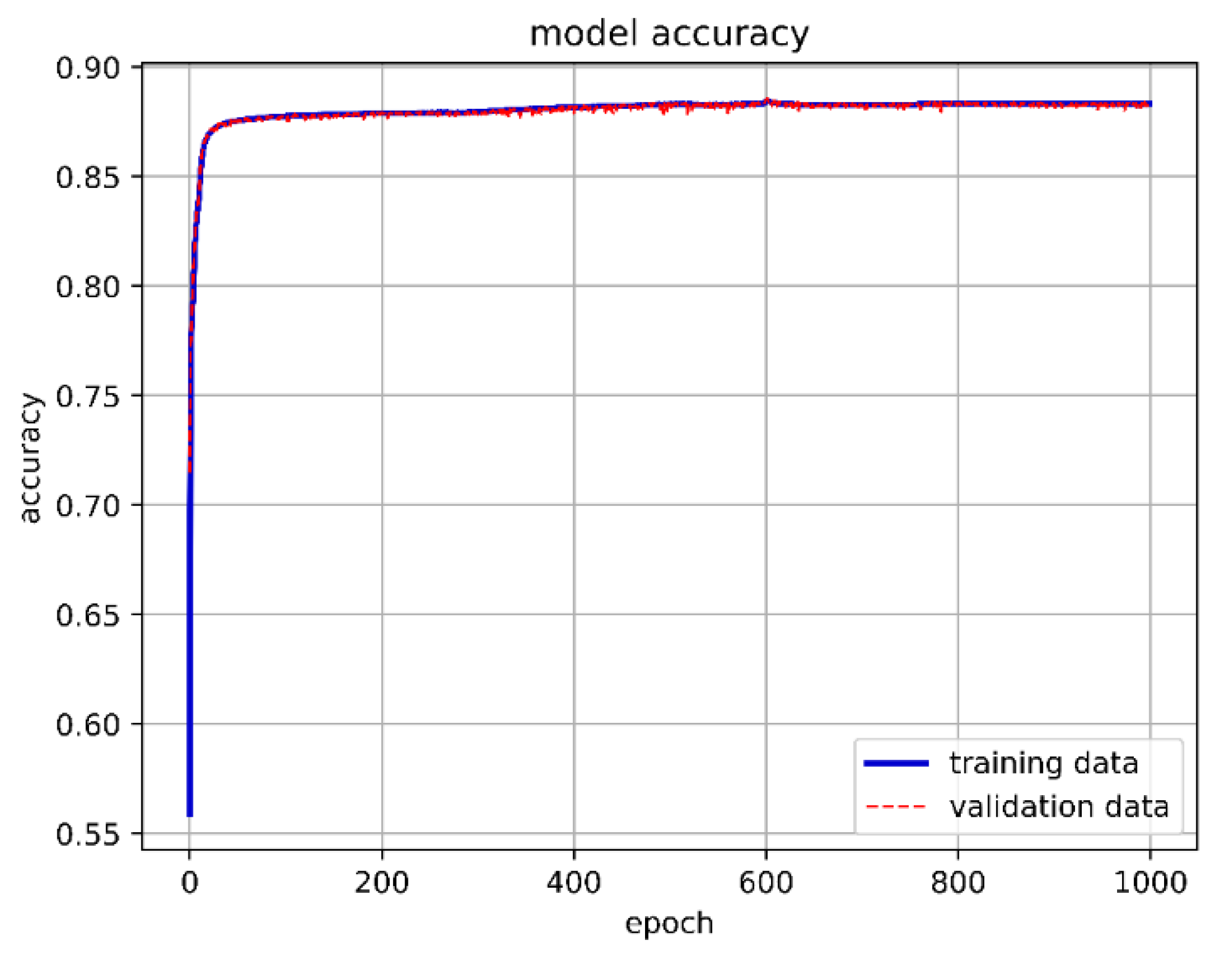
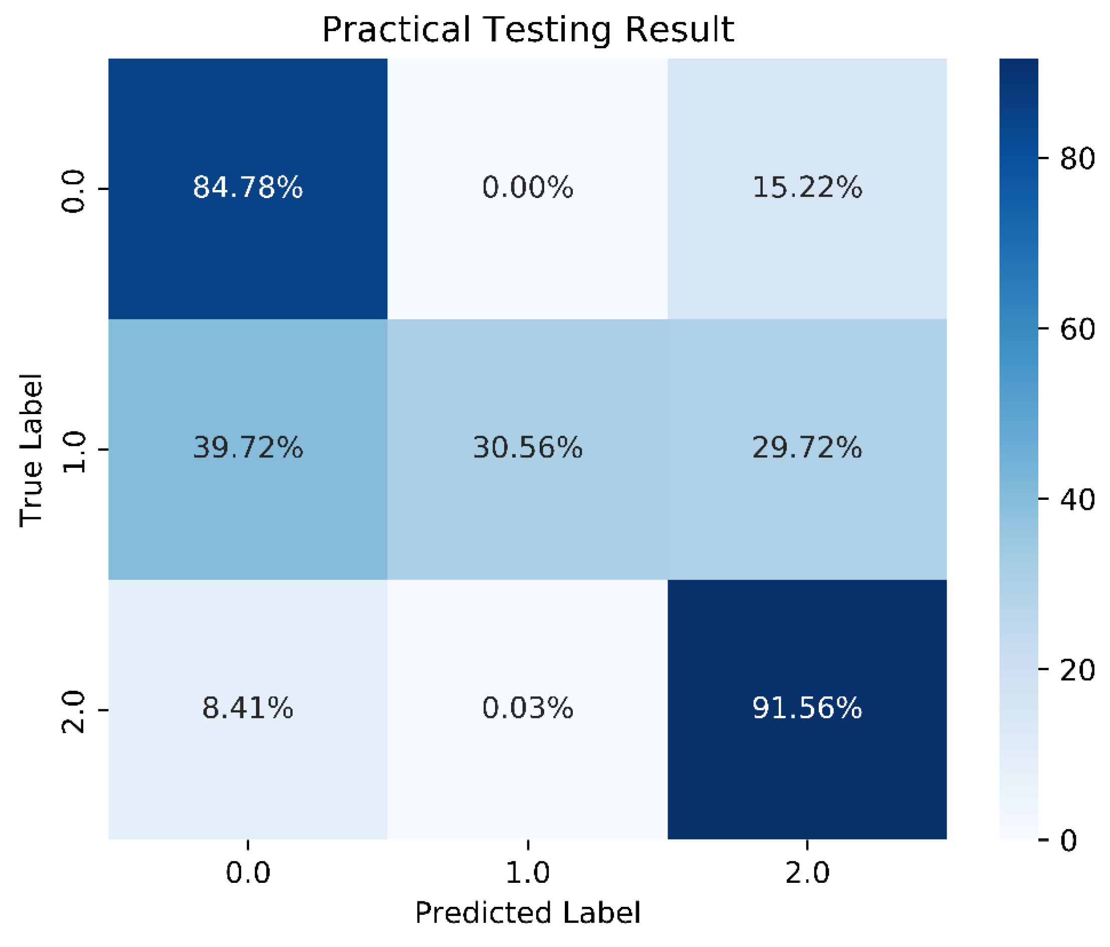
We constructed the DNN with an input layer, a hidden layer, and an output layer. A ReLU function was used as the activation function in the hidden layer. Since our training goal involved three classifications, we used Softmax as the activation function in the output layer. The cross-entropy loss function was chosen for loss calculation. Initially, we set up 10 neurons, with the batch size and epochs adjusted and fixed at 15,000 and 1000, respectively. Although the overall model accuracy reached 88.29%, the accuracy for predicting stable boundaries was only 30.56%. The one-layer DNN training model architecture is shown in Figure 13, 1-layer DNN model accuracy is shown in Figure 14, and 1-layer DNN model loss is shown in Figure 15. The prediction results are shown in Figure 16.
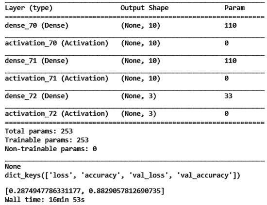
Figure 13.
One-layer DNN training model architecture.
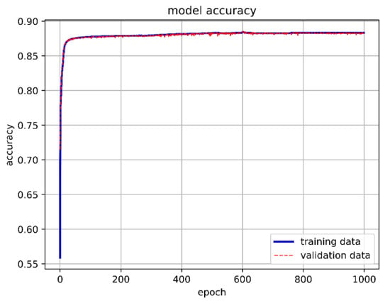
Figure 14.
One-layer DNN model accuracy.
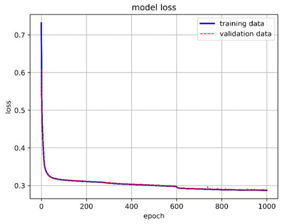
Figure 15.
One-layer DNN model loss.

Figure 16.
Prediction results for the 1-layer DNN model.
The situation arises because there are relatively fewer data points in scenario 1, resulting in this outcome. After various attempts, we decided to adjust the weights using class weights to address the problem of data imbalance. The goal was to ensure the model could better predict the minority class and highlight the importance of different classes, thereby improving model performance and prediction accuracy. However, improper setting of proportions can lead to overfitting and a decrease in accuracy. Ultimately, the weights we decided to use are shown in Figure 17.

Figure 17.
Weight values for different classes.
After adjusting the weights, there was a noticeable improvement in the training data for scenario 1, as shown in Figure 18.
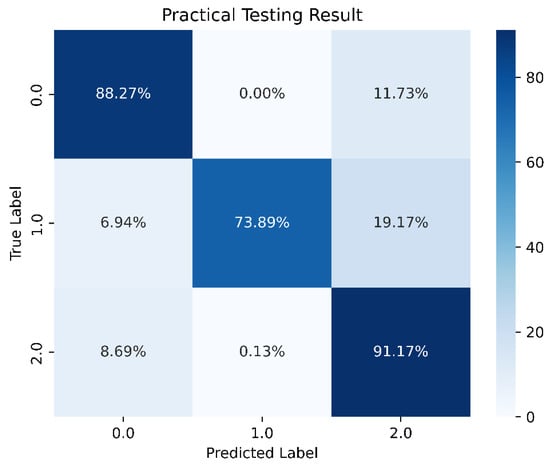
Figure 18.
Predictions after weighting.
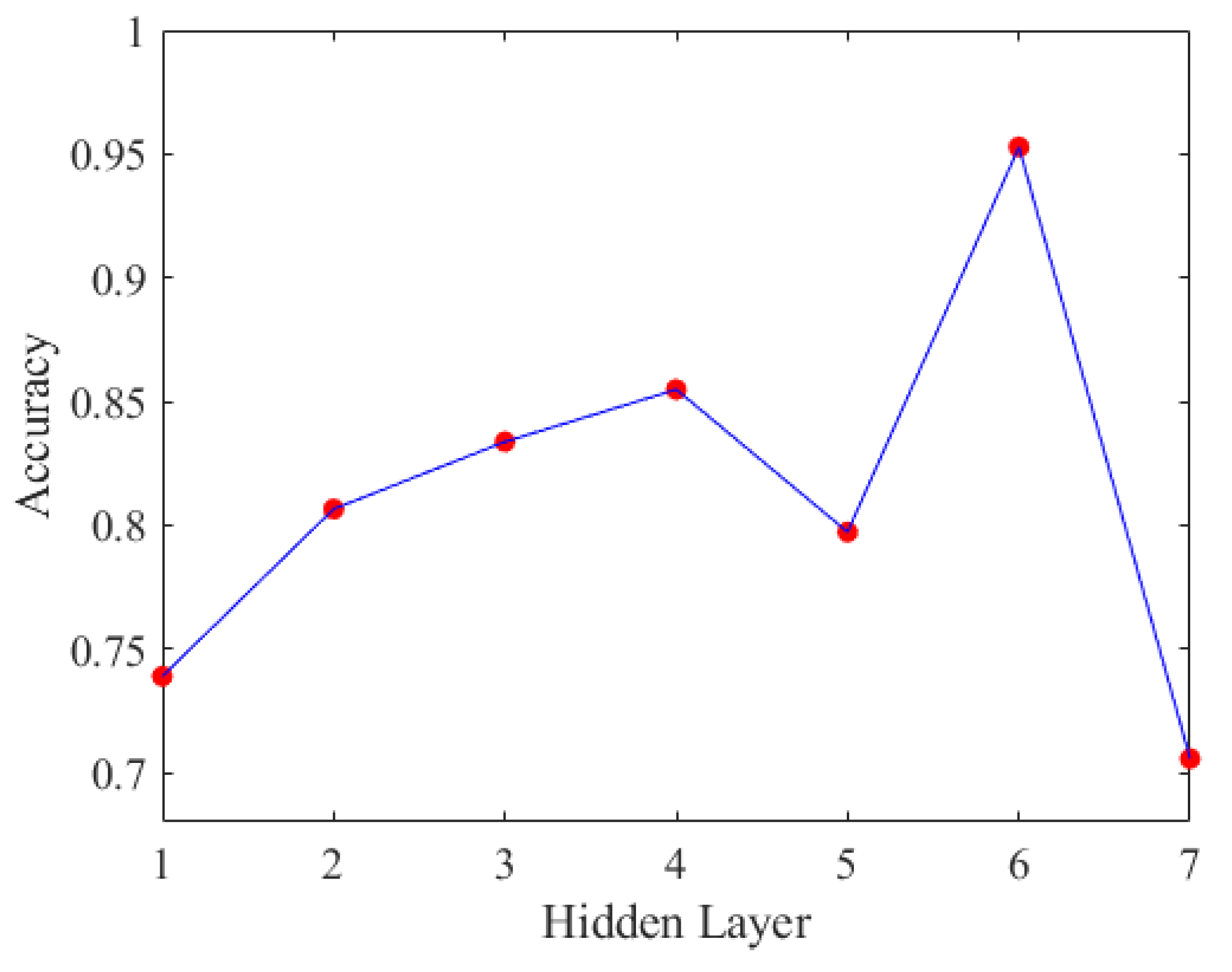
Due to the prediction accuracies for scenarios 0 and 2 already exceeding 90%, we will directly compare the prediction accuracy of scenario 1 across different hidden layers. We experimented with different numbers of hidden layers, using ReLU as the activation function after each hidden layer, and Softmax as the activation function for the output layer. The accuracy results are shown in Figure 19.
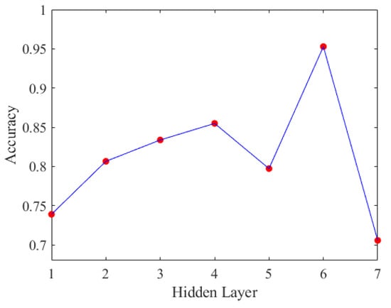
Figure 19.
Accuracy of DNN with different hidden layers.
Based on the displayed prediction accuracy for scenario 1 in Figure 19, it is evident that the optimal number of hidden layers is six. After determining the number of hidden layers, we proceeded to experiment with different numbers of neurons to identify the best deep neural network model, as shown in Figure 20.
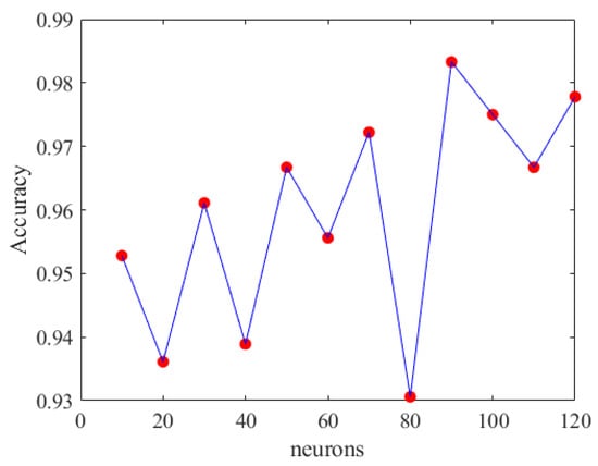
Figure 20.
Accuracy of DNN with different neurons.
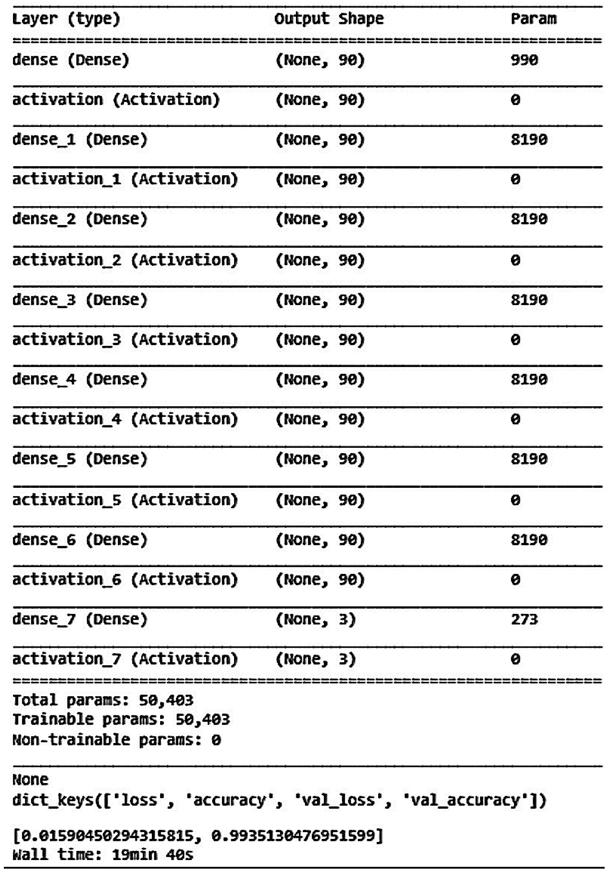
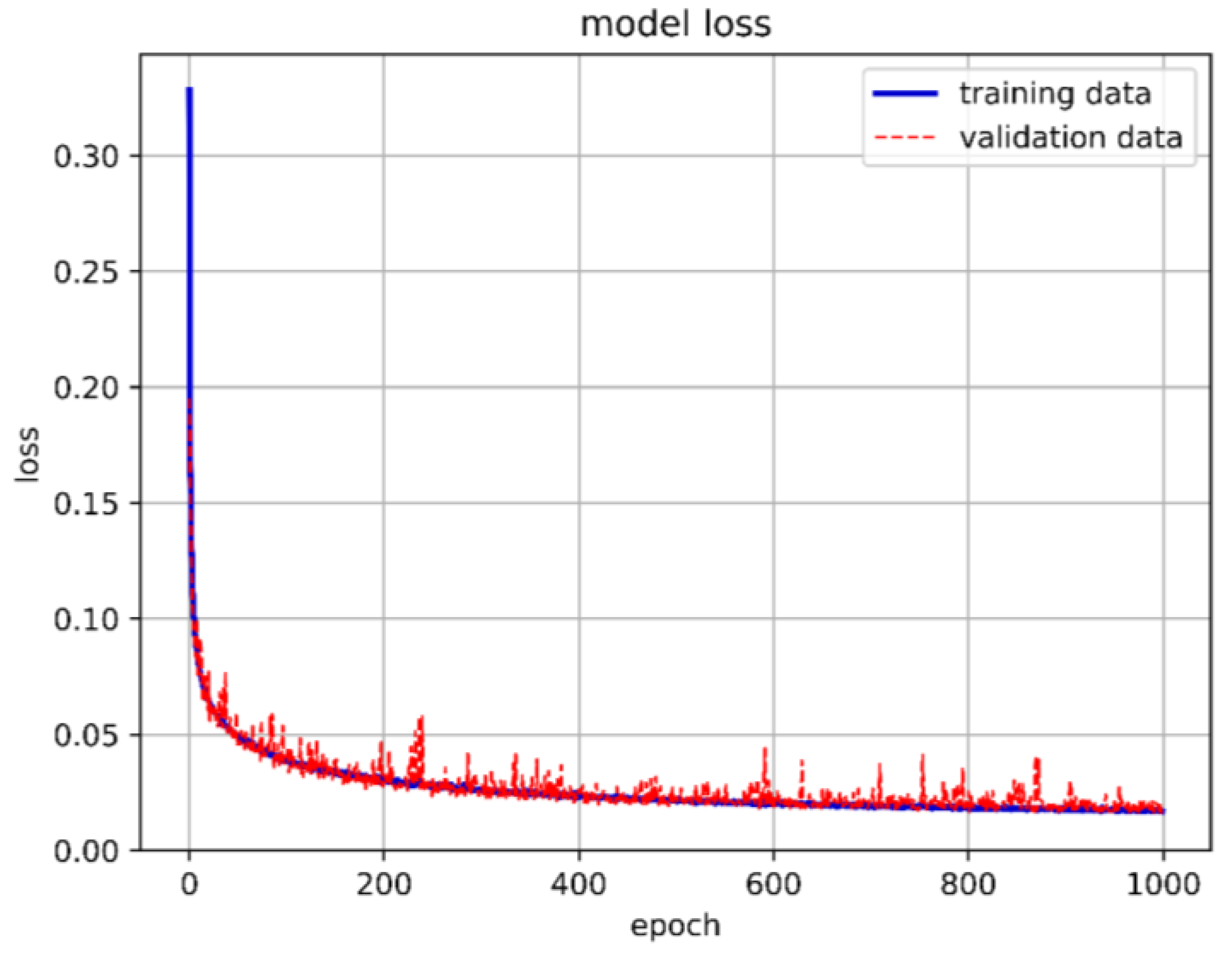
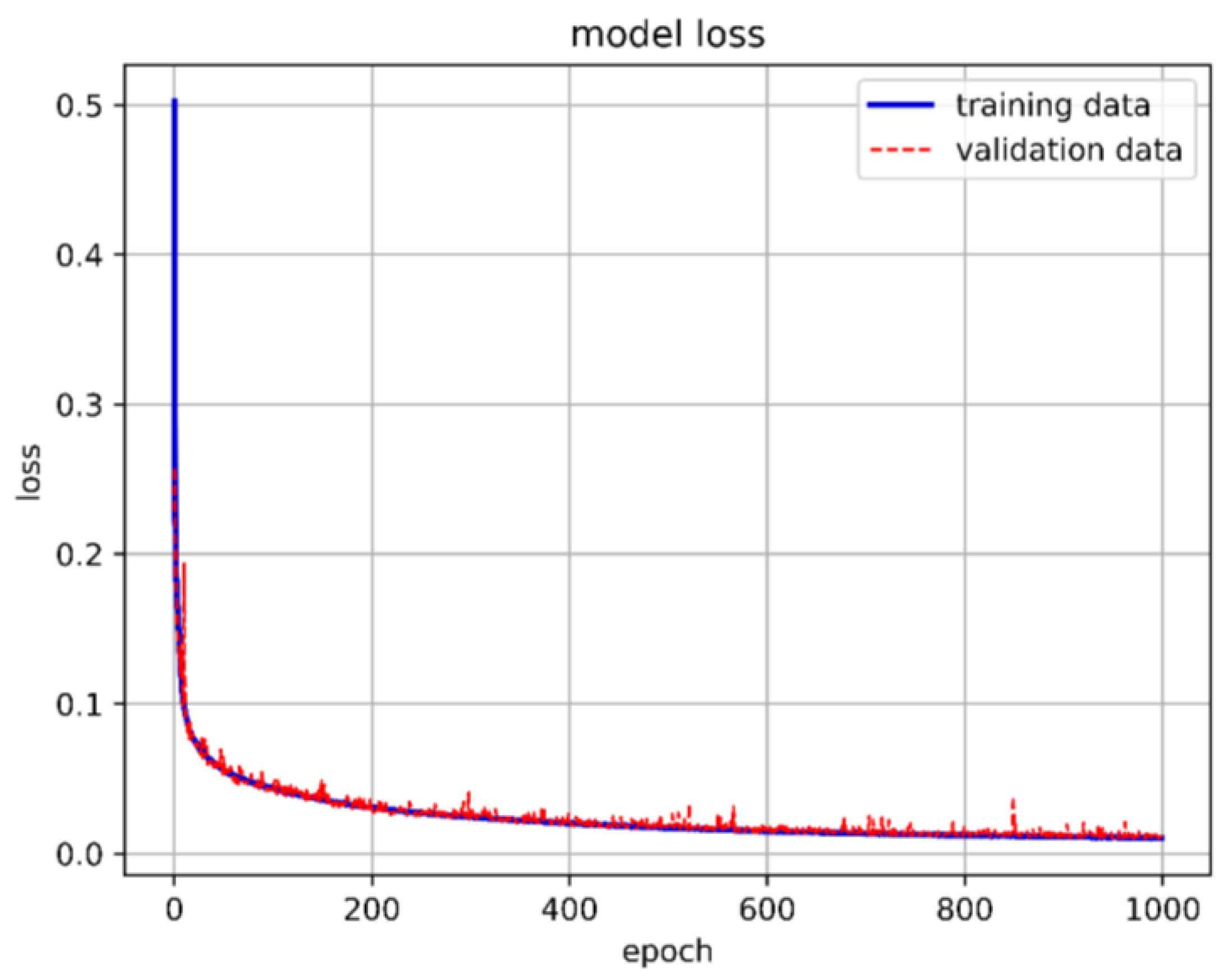
From Figure 20, it can be inferred that selecting appropriate neurons and hidden layers is crucial as it significantly affects the training outcomes. When using 90 neurons per layer, the training prediction achieved an accuracy of 98.89%. Therefore, we chose a DNN model with six hidden layers and 90 neurons each. Figure 21 depicts the optimal DNN model architecture for this study. The training accuracy, loss, and prediction results are shown in Figure 22, Figure 23 and Figure 24, respectively.
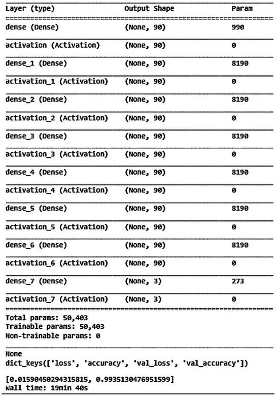
Figure 21.
The best DNN model architecture in this study.
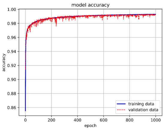
Figure 22.
Training accuracy of the best DNN model in this study.

Figure 23.
Training loss of the best DNN model in this study.
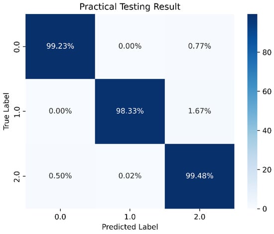
Figure 24.
Prediction of the best DNN model in this study.
4.3. LSTM Model Establishment and Analysis (Divergence, Convergence, and Stable Boundary)
The primary reason for choosing LSTM networks is their ability to effectively handle temporal dependencies and sequential data. Panel flutter phenomena in aerospace structures exhibit significant temporal correlations due to the dynamic nature of the aeroelastic interactions over time. LSTMs are specifically designed to capture and model these long-term dependencies and sequential patterns, which are crucial for accurate predictions in such dynamic systems. With regard to GPR and shallow ANNs, while GPR and shallow ANNs are powerful tools for regression tasks, they are generally not optimized for handling sequential data with complex temporal dependencies. GPR assumes a fixed covariance structure and may struggle with large datasets due to computational constraints. Shallow ANNs, on the other hand, may not capture the intricate temporal relationships as effectively as LSTMs. The LSTM networks are highly effective at modeling complex non-linear relationships within the data, which are inherent in the aeroelastic behaviors of panel flutter. The recurrent nature of LSTMs allows them to maintain and update memory of previous inputs, enabling them to learn and represent the intricate dynamics of the system. The GPR, while flexible, may not scale well with the large dataset used in our study (707,472,000 data points) and may encounter difficulties in modeling very complex non-linear relationships. Shallow ANNs can model non-linearities to some extent but might require significantly more neurons and layers to achieve the same level of performance as LSTMs, which could lead to overfitting and other challenges. The ability of LSTMs to leverage temporal information resulted in more robust and accurate predictions of panel flutter under various flight conditions. Although LSTMs typically require longer training times due to their recurrent structure, the trade-off is justified by their superior performance and generalization capabilities. Our study included measures to balance training time and model accuracy, ensuring efficient training processes. The LSTM networks have been successfully applied to various time-series prediction tasks in engineering and other fields, demonstrating their effectiveness in modeling dynamic systems. By applying LSTMs to predict panel flutter, we leverage a proven technique for capturing the temporal evolution of aeroelastic responses, aligning with the specific requirements of aerospace engineering applications.
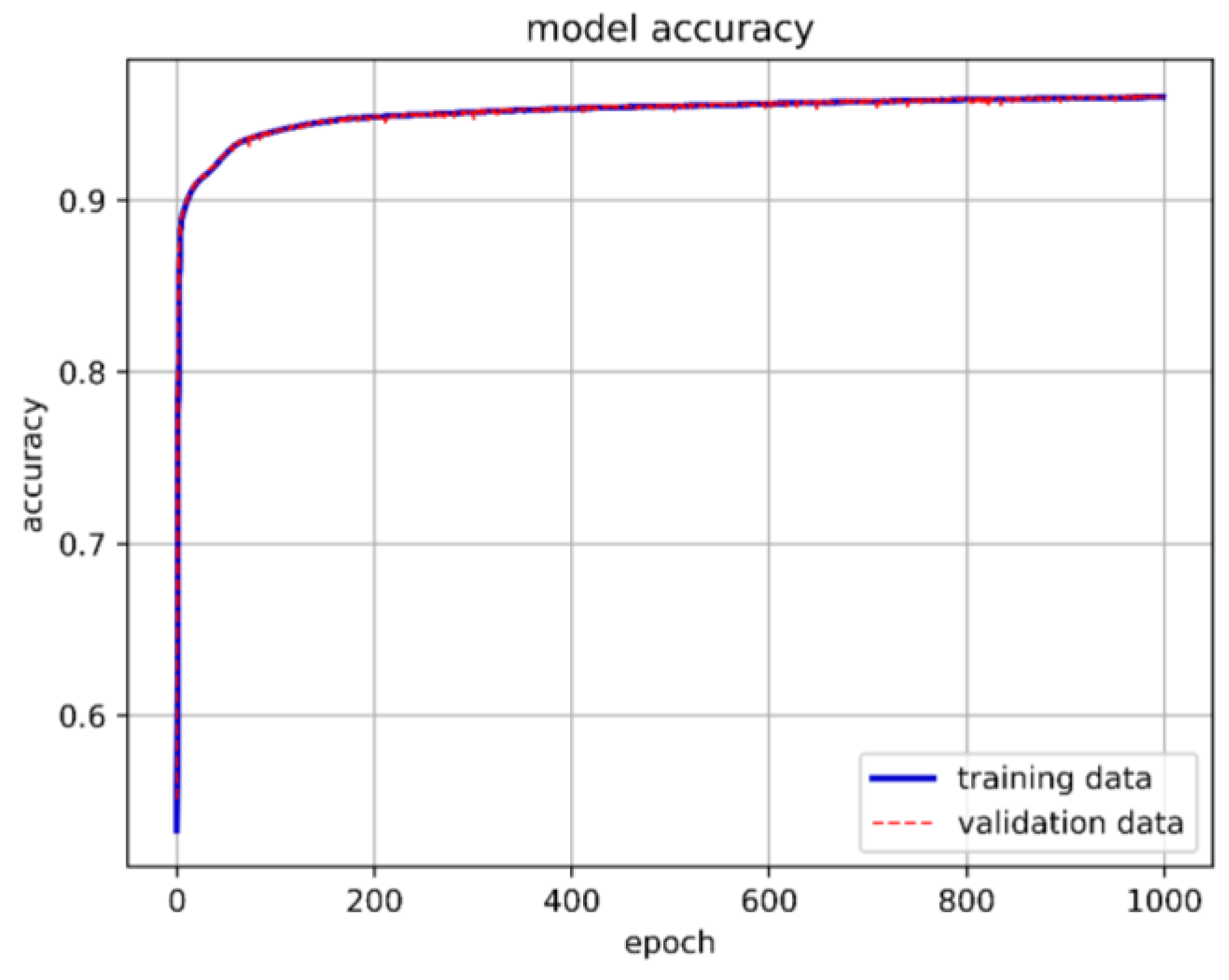
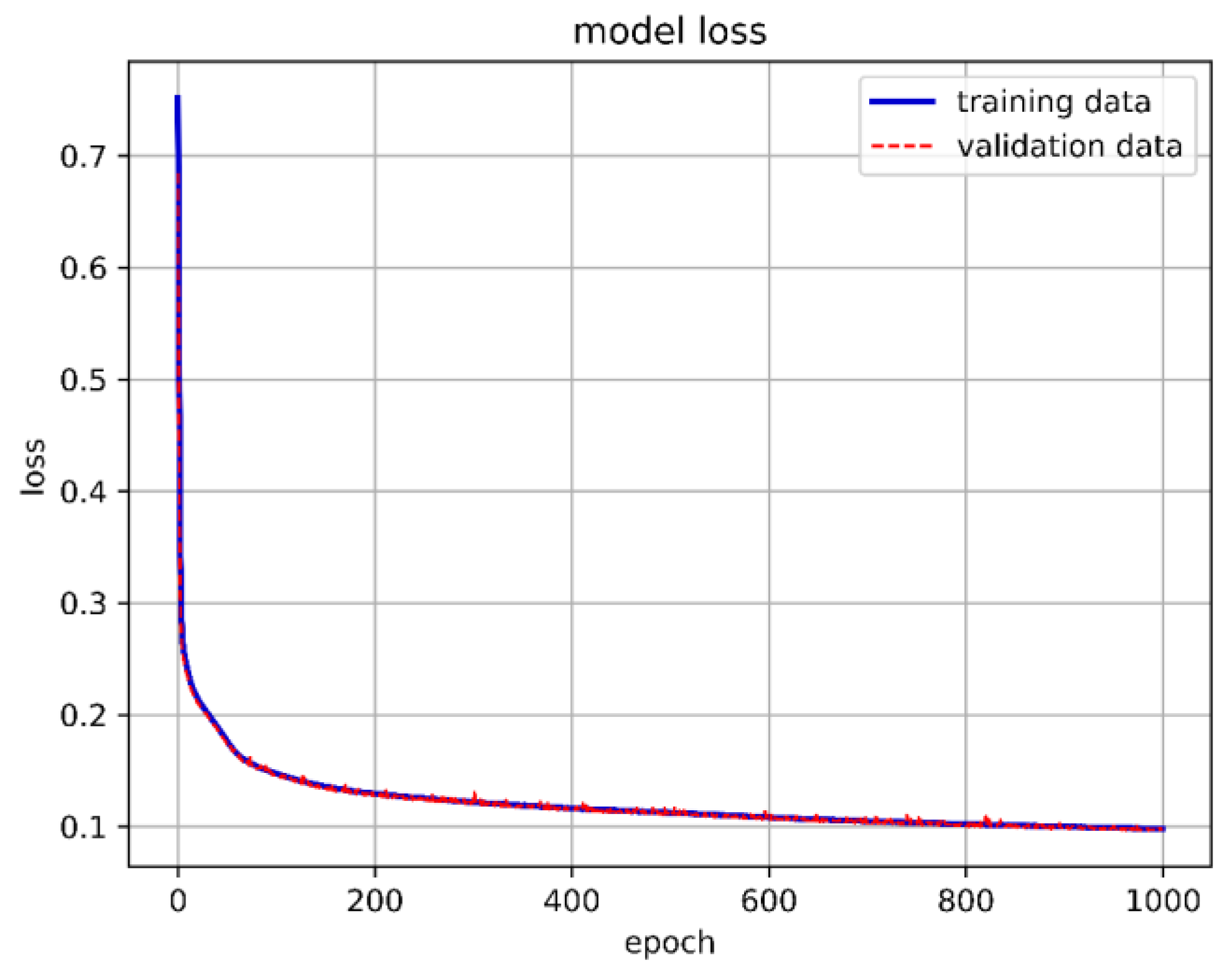
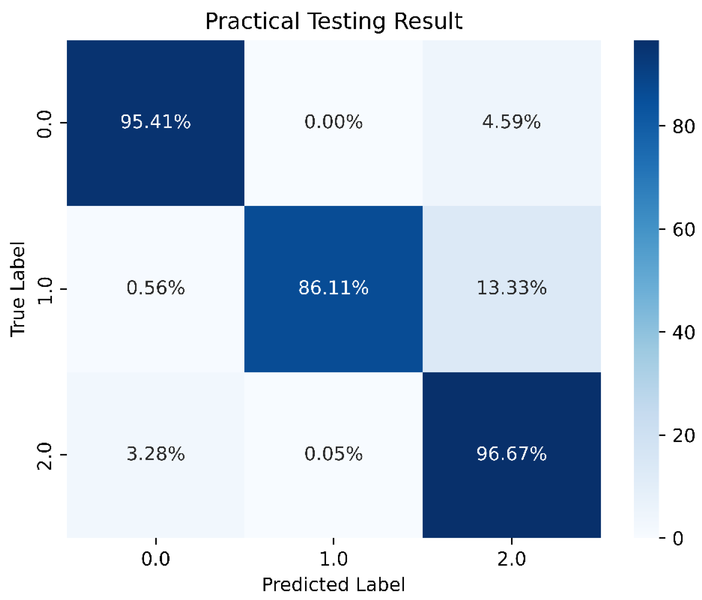
Following the methodology used in Section 4.2, the data were split into 70% for the training set, 25% for the validation set, and the remaining 5% for the test set. For the LSTM architecture, we adopted a simple configuration consisting of one input layer, one hidden layer, and one output layer. We set 10 neurons per layer and a batch size of 15,000. The model underwent training for 1000 epochs with class weights applied similarly. In each hidden layer, ReLU was employed as the activation function, while Softmax was used in the output layer. The model achieved an accuracy of 96.07%, with a prediction accuracy of 86.11% specifically for stable boundaries. These results are illustrated in Figure 25, Figure 26, Figure 27 and Figure 28.

Figure 25.
One-layer LSTM training model architecture.
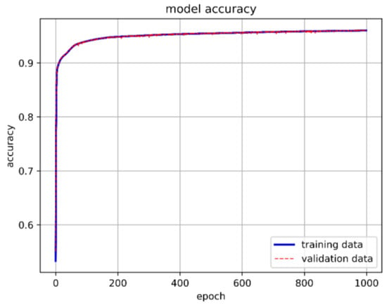
Figure 26.
One-layer LSTM model accuracy.
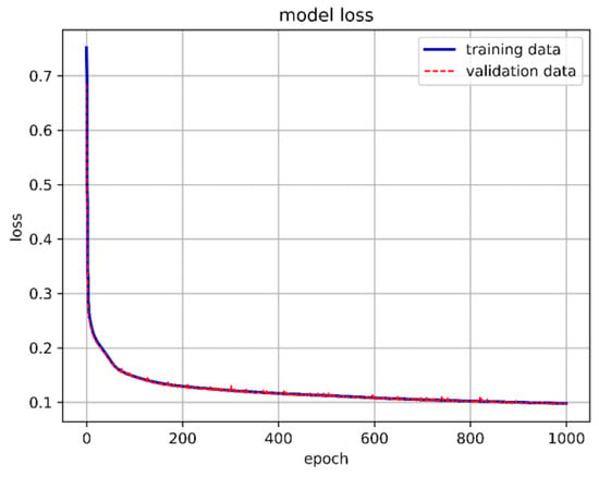
Figure 27.
One-layer LSTM model loss.

Figure 28.
One-layer LSTM prediction results.
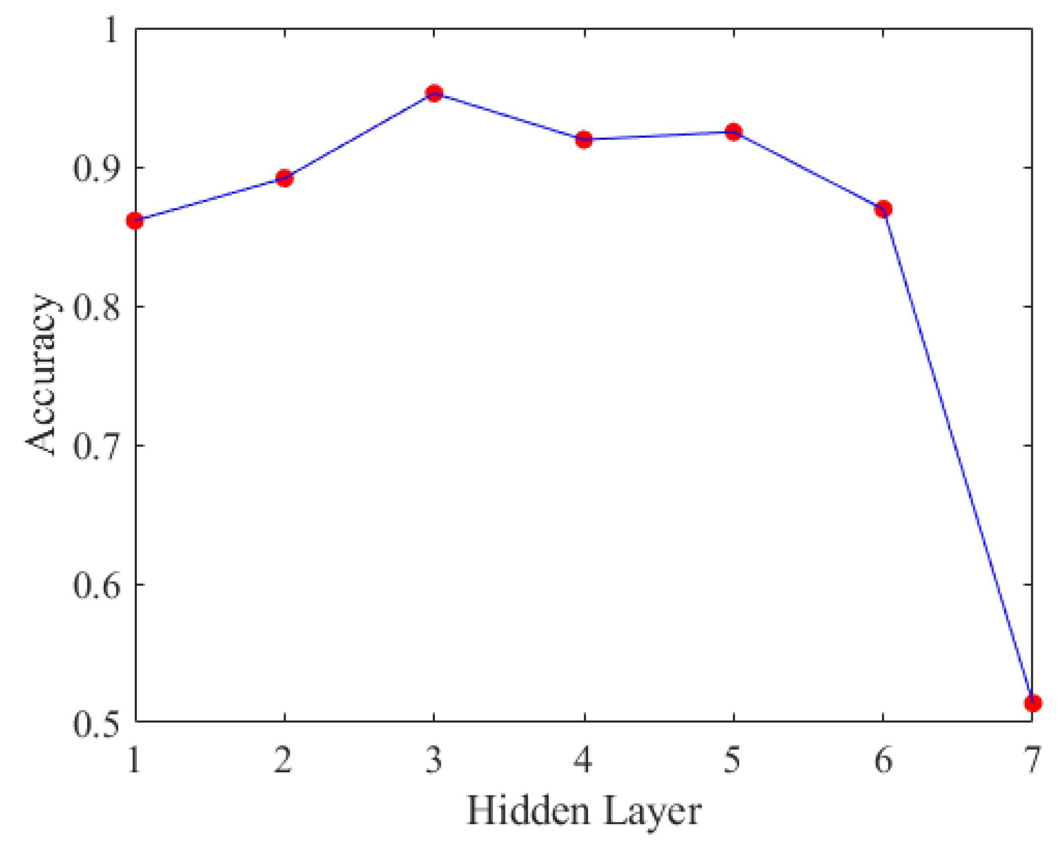
We use the method from Section 4.2, keeping the number of neurons fixed at 10, and test various hidden layer configurations to identify the optimal training model. The results are shown in Figure 29.
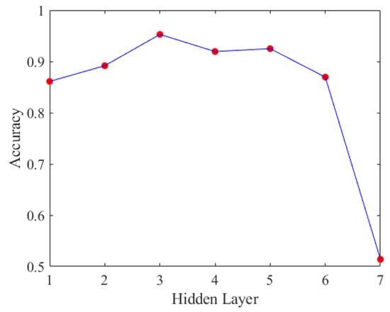
Figure 29.
Accuracy of different hidden layers of LSTM.
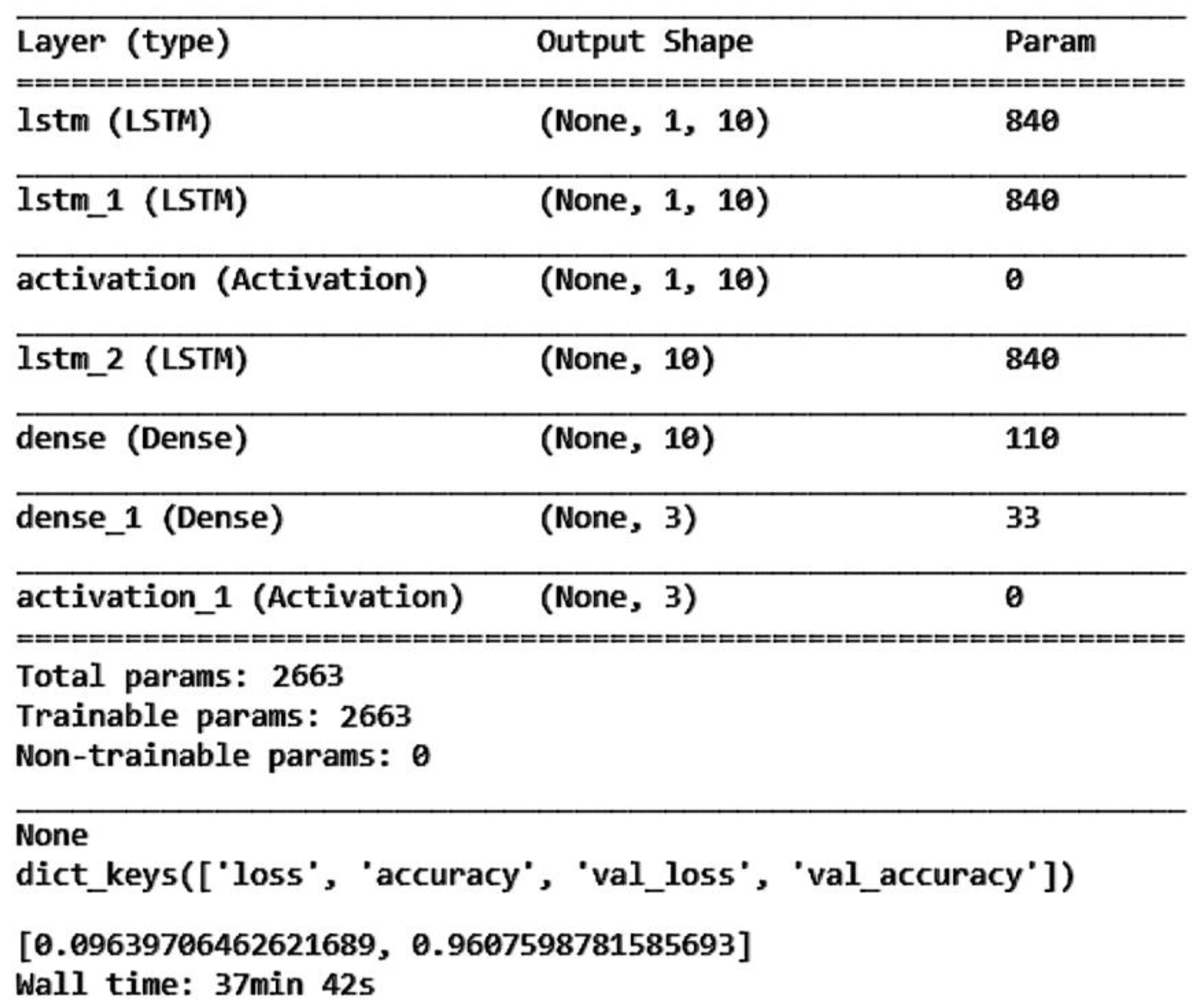
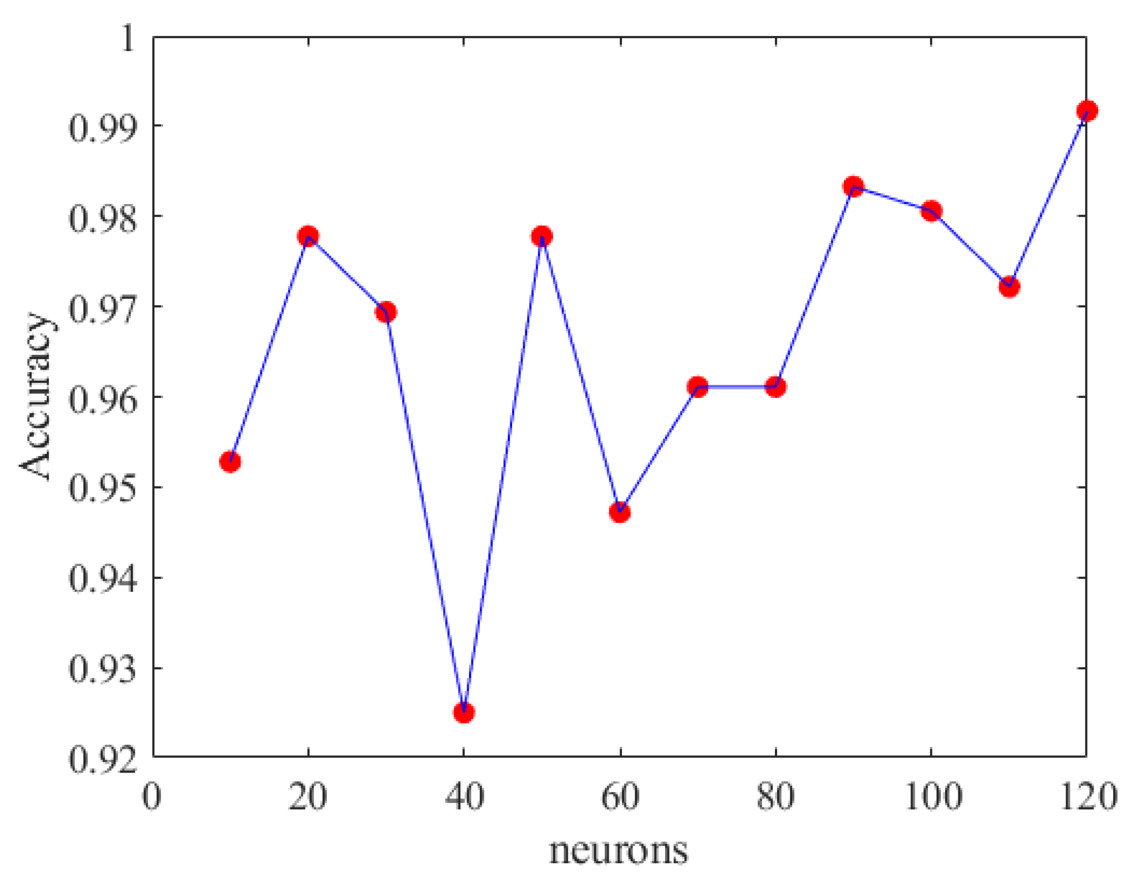
Based on the assessment in Figure 29, we ultimately decided to use three LSTM hidden layers. Keeping these three layers fixed, we then adjusted the number of neurons to find the optimal model.
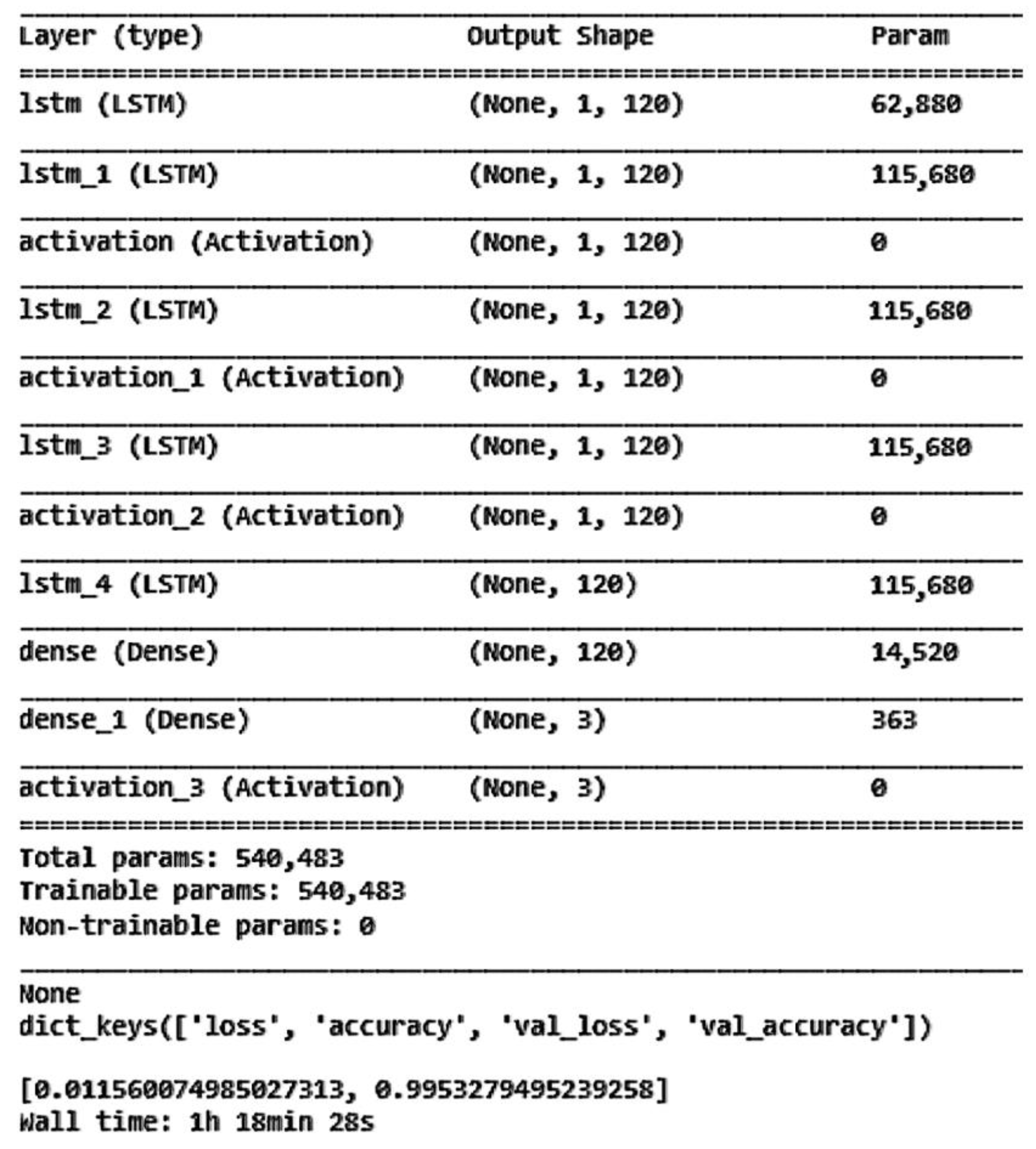
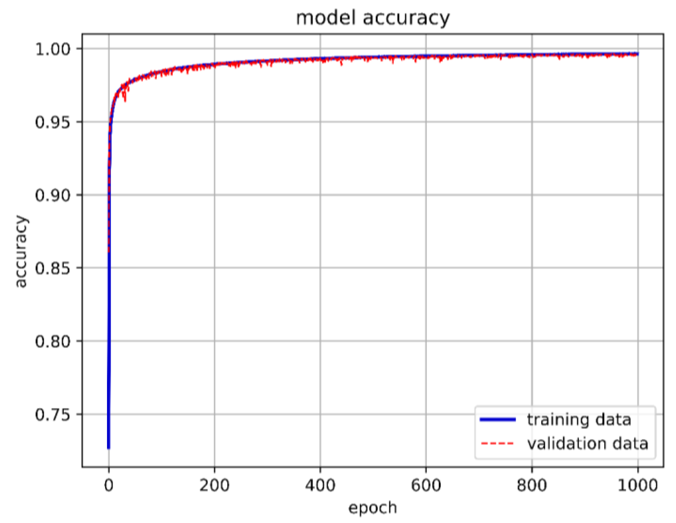
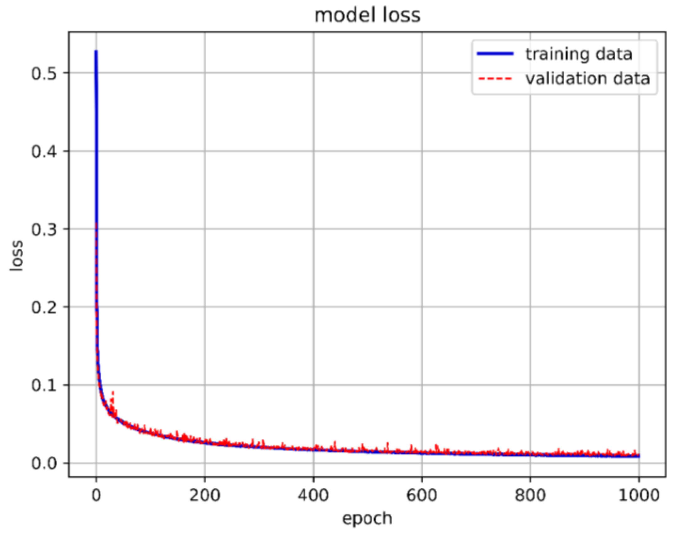
From Figure 30, it can be seen that having 120 neurons in the three LSTM hidden layers yields the highest accuracy. Therefore, we chose to use 120 neurons for our long short-term memory deep learning model. Figure 31 shows the architecture of the optimal long short-term memory model and the training accuracy, loss, and prediction results are shown in Figure 32, Figure 33 and Figure 34.
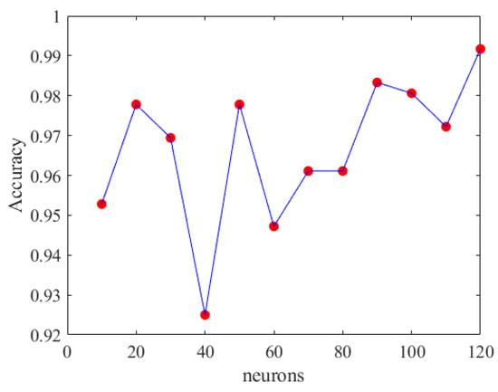
Figure 30.
Accuracy of different neurons in LSTM.

Figure 31.
The best LSTM model architecture in this study.
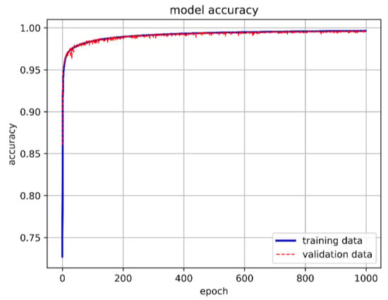
Figure 32.
The best LSTM model training accuracy in this study.
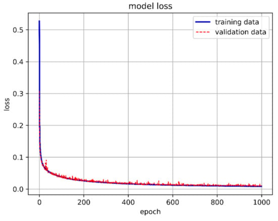
Figure 33.
The best LSTM model training loss in this study.
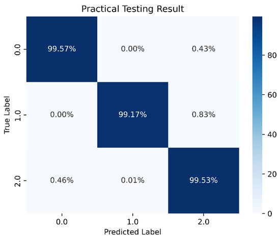
Figure 34.
The best LSTM model prediction in this study.
4.4. LSTM-NN Model Development and Analysis (Divergence, Convergence, and Stability Boundary)
While the DNN and LSTM models both achieved over 98% accuracy, we aimed to see if even higher accuracy could be achieved. Therefore, we experimented with adding neural network hidden layers to the LSTM model. Using the same LSTM approach as mentioned in Section 4.3, we first established the input layer and divided the data into 70% training set, 25% validation set, and the remaining 5% test set. Following Section 4.2, we kept the class weight, number of neurons at 10, epoch, and batch size the same as in the previous sections. Table 2 shows the accuracy, model loss, and stable boundary prediction accuracy for different hidden layer configurations. The model with three LSTM layers and one NN hidden layer achieved the highest accuracy and lowest loss.

Table 2.
Model accuracy, loss, and prediction accuracy of different hidden layers.
After selecting the model architecture, we adjusted the number of neurons. As in the previous Sections, since the accuracy for scenarios 0 and 2 reached 99%, we compared the prediction accuracy for the stability boundary.
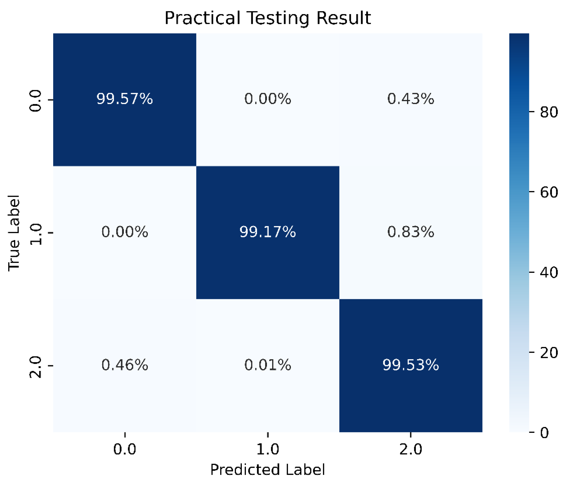
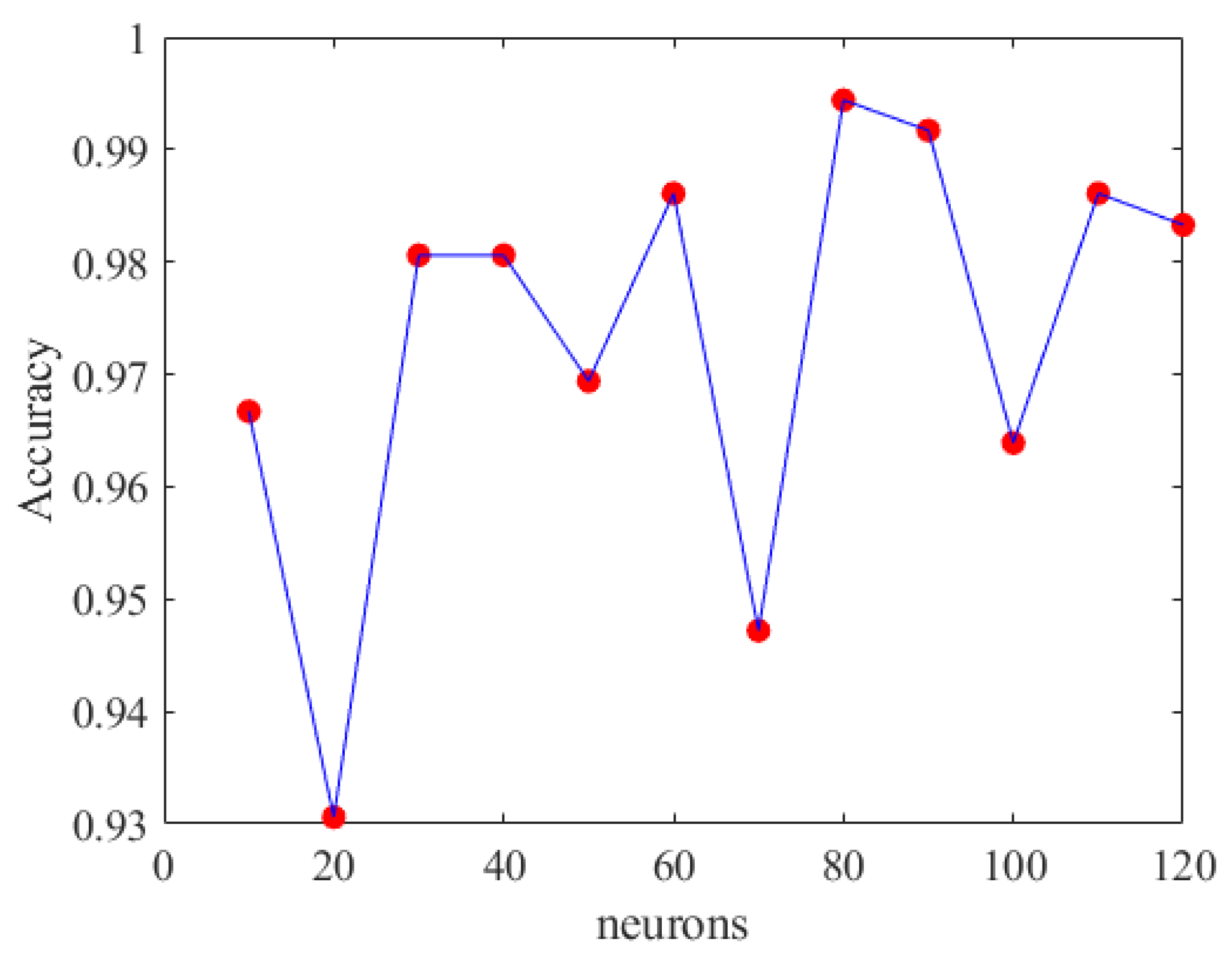
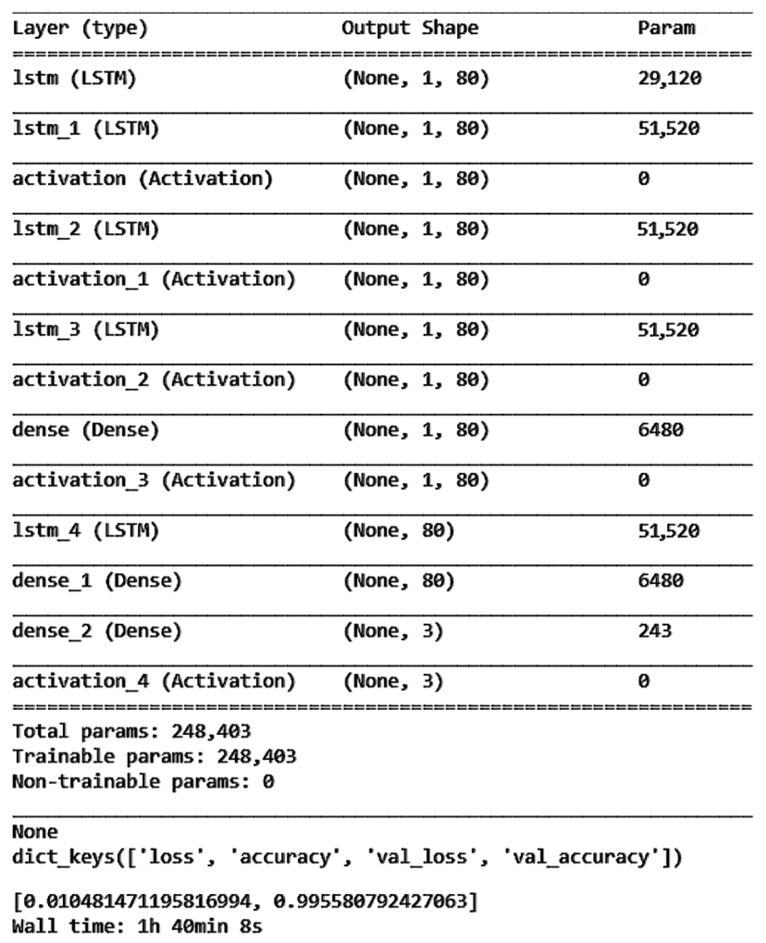
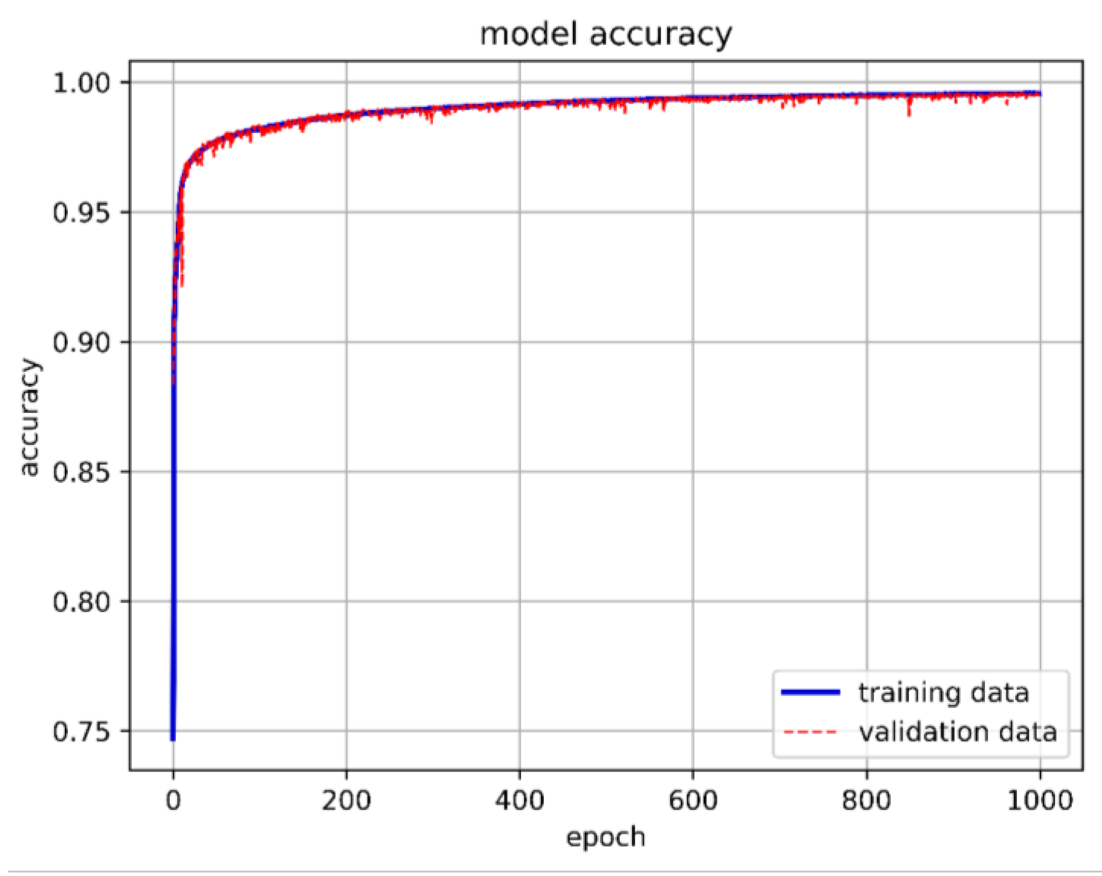
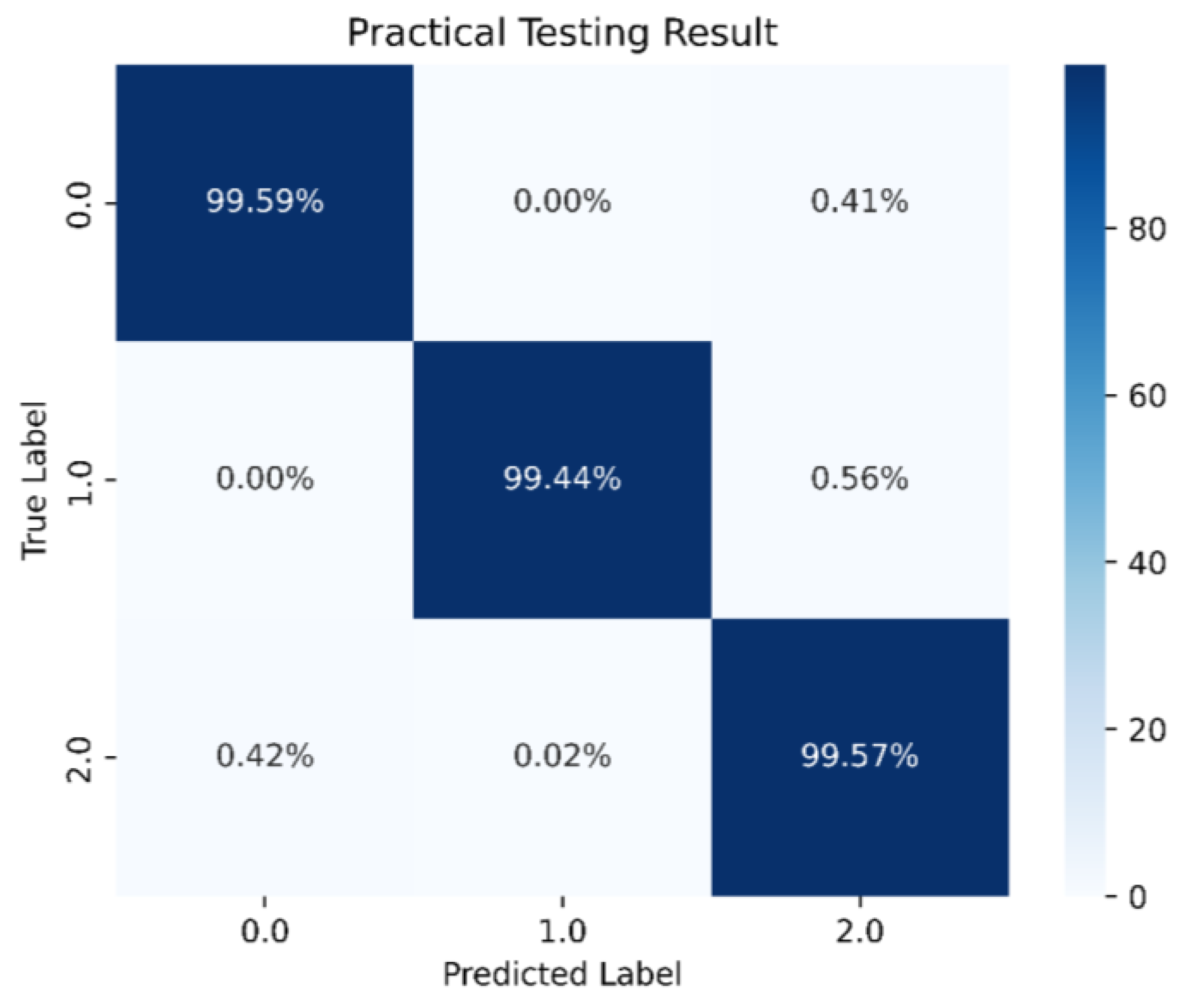
When the neuron count was set to 80, the prediction accuracy for the stability boundary reached 99.44%, as shown in Figure 35. Therefore, the final model architecture set the number of neurons in the hidden layer to 80. Figure 36 shows the LSTM-NN model architecture for this study, with training accuracy, loss, and prediction results shown in Figure 37, Figure 38 and Figure 39.
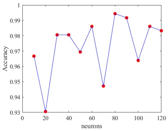
Figure 35.
LSTM-NN accuracy of different neurons.
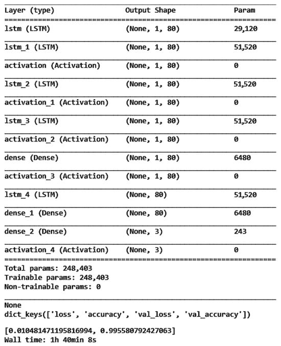
Figure 36.
The best LSTM-NN model architecture in this study.
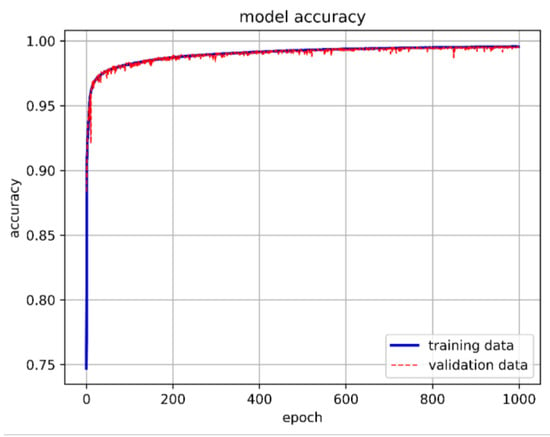
Figure 37.
The best LSTM-NN model training accuracy in this study.

Figure 38.
The best LSTM-NN model training loss in this study.
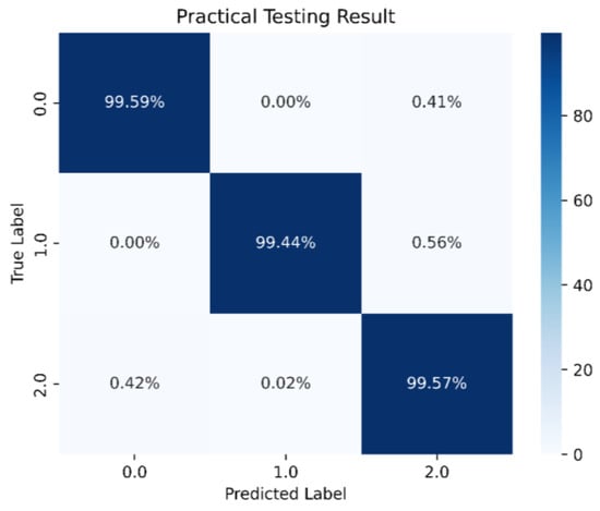
Figure 39.
Best LSTM-NN model prediction in this study.
In this study, we explored various deep learning architectures, specifically Deep Neural Networks (DNN), Long Short-Term Memory (LSTM), and Long Short-Term Memory Neural Networks (LSTM-NN). Each architecture was tested with different configurations of hidden layers and neurons to understand their impact on performance. We investigated shallow networks (fewer hidden layers) and deep networks (more hidden layers) to determine the optimal depth for each model (Figure 19 and Figure 29). Shallow networks are typically faster to train and less prone to overfitting, while deep networks can capture more complex patterns but may require more regularization. Our findings indicated that increasing the number of hidden layers generally improved the models’ ability to learn complex patterns from the data. However, beyond a certain point, additional layers led to diminishing returns in accuracy and increased the risk of overfitting. For example, DNN and LSTM models showed significant improvements up to 4–5 hidden layers but adding more layers resulted in marginal gains or even reduced performance due to overfitting. We also varied the number of neurons (Figure 20 and Figure 30) in each hidden layer to study their impact on performance. A higher number of neurons allows the model to learn more detailed representations of the input data but can also increase the risk of overfitting. Our present studies revealed that an optimal range of neurons provided the best balance between model complexity and performance. Models with too few neurons struggled to capture the underlying patterns, while those with too many neurons tended to overfit the training data. For DNNs, we observed that 3–5 hidden layers with 100–200 neurons per layer achieved the best performance. These configurations provided sufficient capacity to learn the complex aeroelastic behaviors without overfitting. LSTM models benefited from having between two and four LSTM layers with 50–150 neurons per layer. This architecture effectively captured temporal dependencies and complex non-linear relationships in the data, making it ideal for predicting flutter Mach numbers. The LSTM-NN models, which combine LSTM and feedforward layers, showed optimal performance with two to three LSTM layers followed by one to two fully connected layers, each with 100–150 neurons. This hybrid architecture leveraged the strengths of both LSTM and DNN models, providing high accuracy in both classification and regression tasks. We compared the performance of different architectures using key metrics such as Mean Squared Error (MSE), R-square values, and training/validation accuracy. These comparisons were conducted across multiple datasets and configurations to ensure robustness. The empirical results showed that while deeper models and those with more neurons generally provided better performance, there was a clear threshold beyond which additional complexity did not yield significant gains. For instance, LSTM-NN models consistently outperformed pure DNN and LSTM models in classification tasks, while LSTM models excelled in regression tasks with fewer layers and neurons. The choice of model architecture should consider the specific requirements of the task at hand. For tasks involving sequential data and temporal dependencies, LSTM and LSTM-NN models are more suitable. For tasks requiring high classification accuracy, hybrid architectures like LSTM-NN provide the best results.
4.5. Model Comparison and Analysis (Divergence, Convergence, and Stability Boundary)
Next, we will compare the advantages and disadvantages of the three different algorithms mentioned earlier. Table 3 compares the best model architecture, training time, model accuracy, model loss, and prediction accuracy for the three different scenarios. From Table 3, it is evident that although the prediction accuracy for scenarios 0 and 2 exceeds an impressive 99%, the DNN’s accuracy for scenario 1 is only 98.33%. In contrast, both the LSTM and LSTM-NN models achieve over 99%. Given the relative computational complexity of LSTM hidden layers compared to DNN hidden layers, adding neural network hidden layers can enhance data learning. However, this increased complexity results in significantly longer training times compared to the DNN. The higher accuracy of LSTM-NN compared to DNN and LSTM is demonstrated in our study through the detailed performance metrics provided in Figure 24, Figure 35 and Figure 39, as well as Table 3. These results illustrate how LSTM-NN consistently achieved better predictive accuracy and model performance. The architectural advantages of LSTM-NN, such as its ability to capture long-term dependencies and sequential patterns, contribute to its higher accuracy in predicting panel flutter under various flight conditions.

Table 3.
Comparison of different algorithms for the best results in this study.
Our study aims to develop and validate DL models using a large dataset generated from a simplified panel plate model. This approach allowed us to create a total of 707,472,000 data points, providing a comprehensive basis for training and evaluating the DL models. We recognize the importance of comparing our DL models with high-fidelity CFD-FEM systems to further validate their accuracy. However, such comparisons were beyond the scope of the current study due to resource and time constraints. The decision to use a simplified panel model was driven by the need to explore the potential of DL techniques in predicting panel flutter efficiently. While CFD-FEM coupled systems offer high accuracy, our goal was to demonstrate the feasibility of using DL models as a computationally efficient alternative for the initial design and analysis phases. Although direct comparisons with CFD-FEM systems were not conducted, we have ensured rigorous verification and validation of our DL models using the extensive dataset generated. The performance metrics and results provided in Figure 24, Figure 35 and Figure 39, as well as Table 2 and Table 3, demonstrate the robustness and accuracy of our models.
4.6. Analysis of Flutter Mach Number Predictions Using Different Models
Using the number of hidden layers and neurons determined in Section 4.2, we trained the data for the flutter speed of small panels separately. We used the same model architecture as before to train and compare the performance of different algorithms. The data were split into 70% training set, 25% validation set, and 5% test set. The input features were the aspect ratio of the small panel, the decay rate (), longitudinal load (), frequency (), and total damping (gT). The label was the Mach number at which panel flutter occurs. Table 4 compares the Mean Squared Error (MSE) and R-square values of DNN, LSTM, and LSTM-NN algorithms.

Table 4.
Comparison of different algorithms for flutter Mach number.
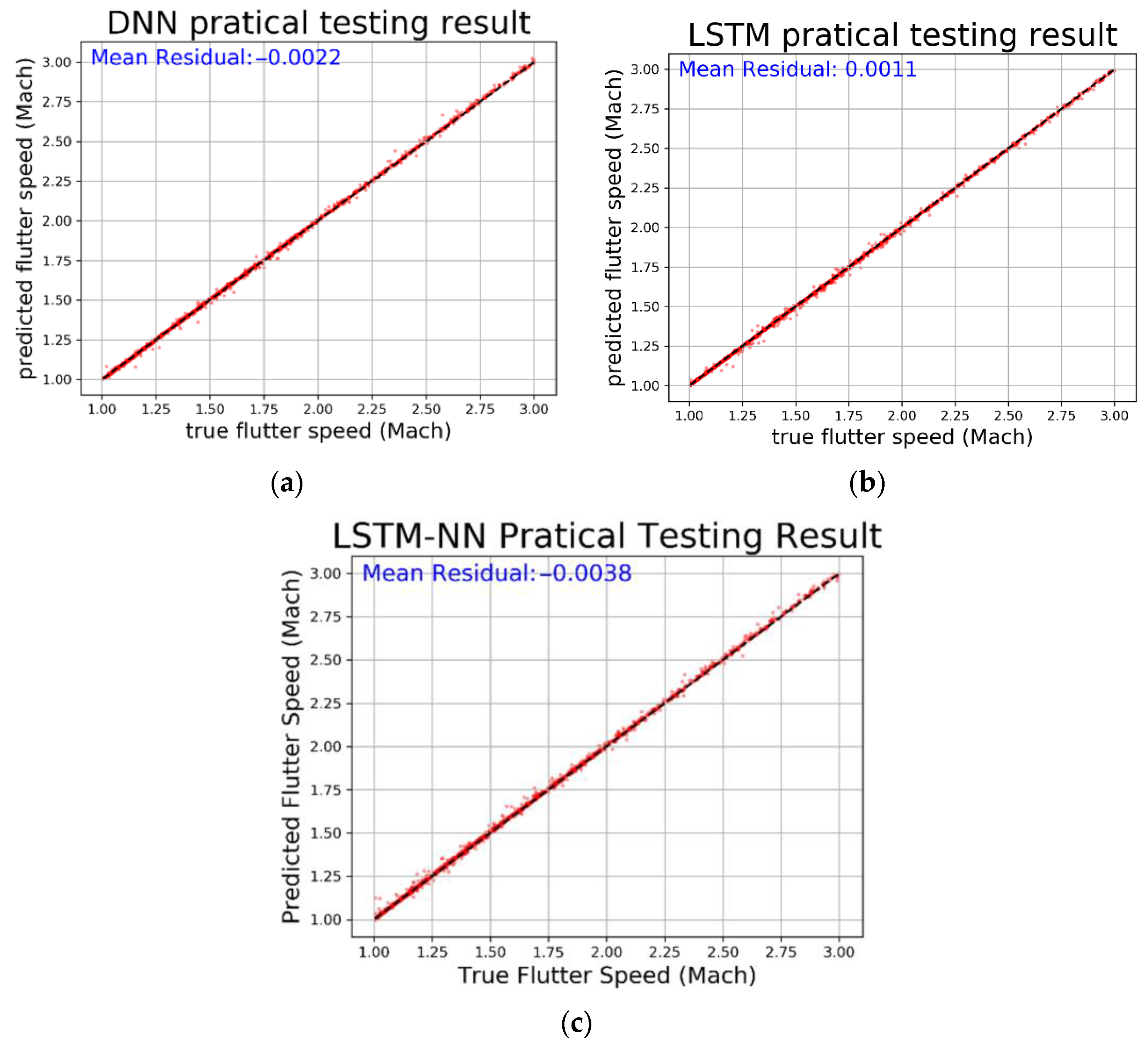
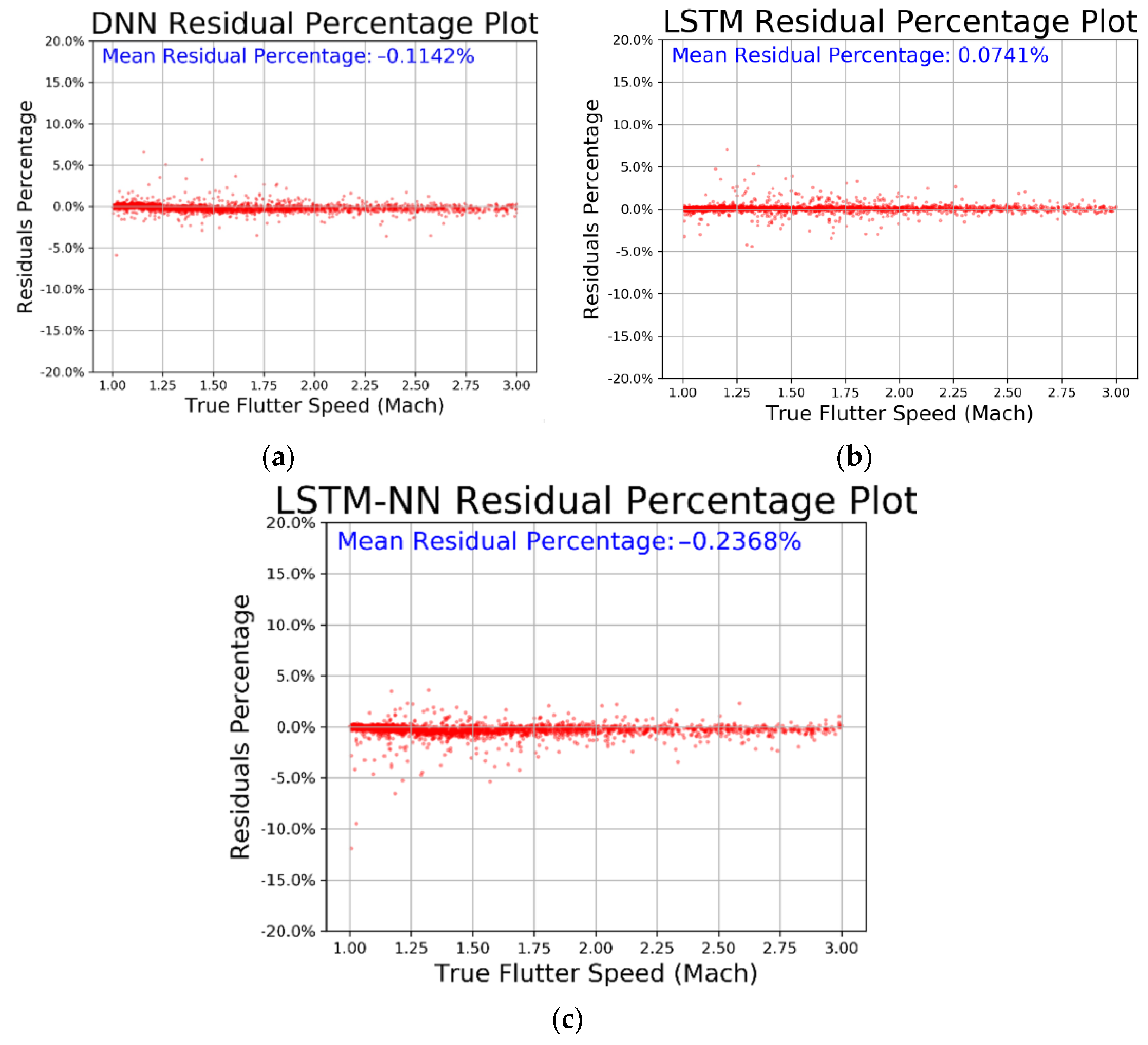
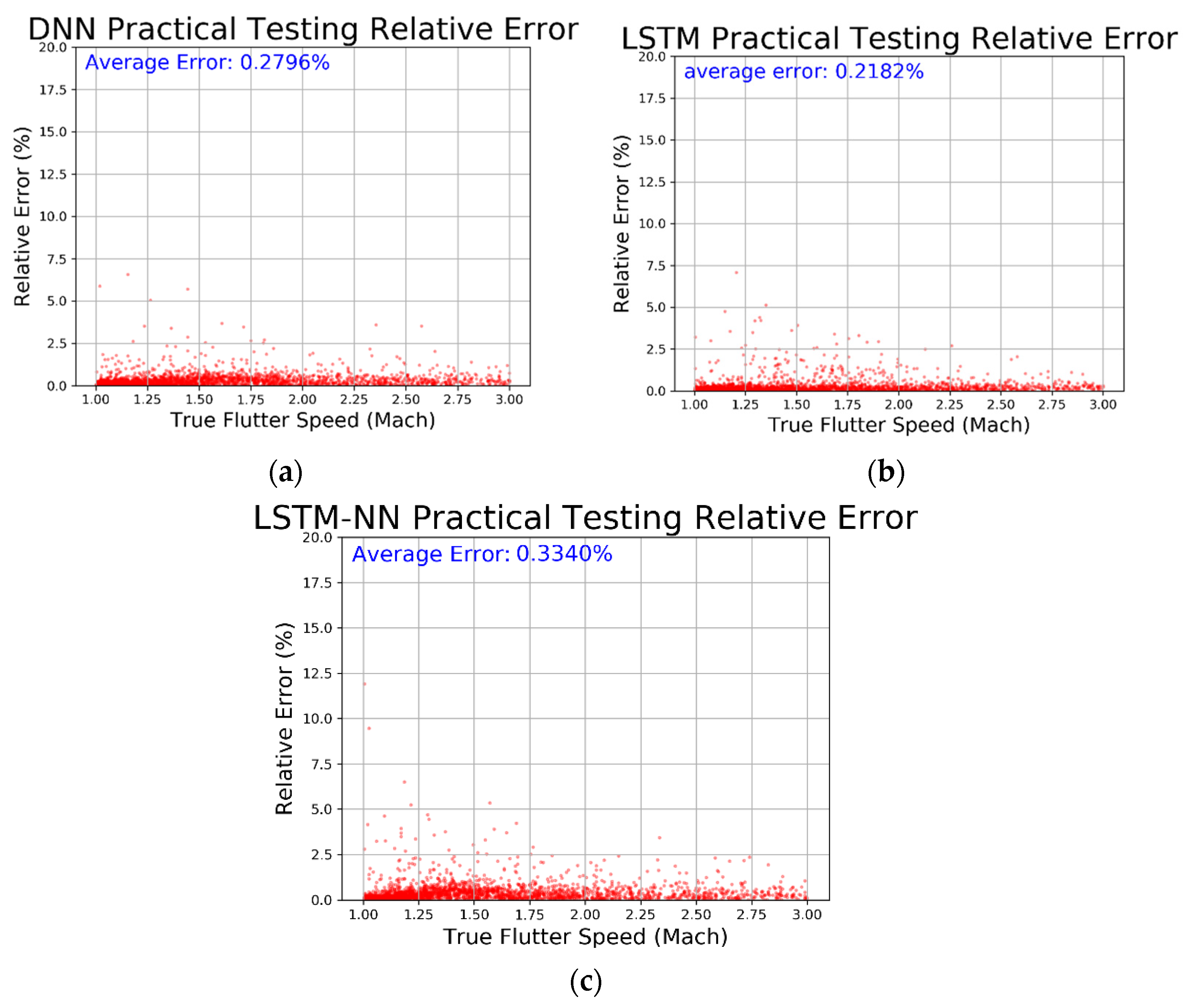
From Table 4, we can see that all three models have very low MSE values and R-square values very close to 1, indicating that the models have converged well and fit the data accurately. We then compared the prediction results, residual percentage, and relative error of the different algorithms for easier comparison. In Figure 40, the horizontal axis represents the actual values and the vertical axis represents the predicted values. The dashed line represents the baseline where the actual value equals the predicted value. In Figure 41, the horizontal axis represents the actual values and the vertical axis represents the residual percentage. In Figure 42, the horizontal axis represents the actual values and the vertical axis represents the error percentage. From the comparison results in the figures, we can see that the LSTM performs better across all three figures and has lower MSE and higher R-square values. The average relative error is as low as 0.2182%.
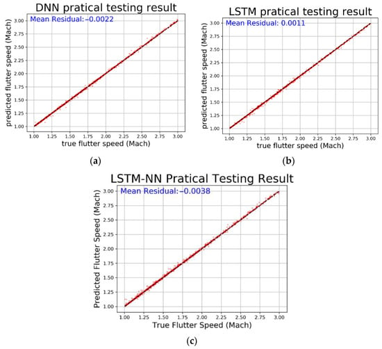
Figure 40.
Prediction and average residual value with regard to (a) DNN, (b) LSTM, and (c) LSTM-NN.

Figure 41.
Prediction residual percentage regarding (a) DNN, (b) LSTM, and (c) LSTM-NN.
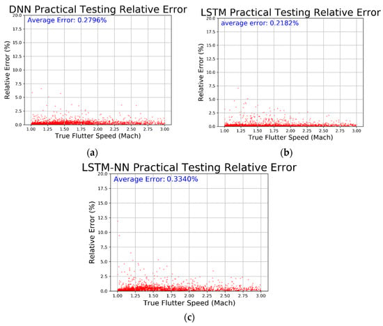
Figure 42.
Relative error regarding (a) DNN, (b) LSTM, and (c) LSTM-NN.
Our dataset comprises 707,472,000 data points, capturing a wide range of flight conditions, panel configurations, and other variables. This extensive dataset helps ensure that the models are trained on diverse scenarios, reducing the risk of overfitting to any specific subset of data. Despite using 5% of the dataset for testing, this still amounts to approximately 35,373,600 data points, providing a substantial and representative test set to evaluate model performance. We divided our dataset into distinct training, validation, and test sets. This approach allows us to monitor the model’s performance on unseen data and adjust hyperparameters to reduce overfitting. In addition to the above techniques, we implemented a weighting strategy to adjust the importance of different data points during training (Figure 17). Weighting helps in managing the influence of varying data points, ensuring that the model captures significant patterns without being overly influenced by outliers. This approach enhances the model’s ability to learn from diverse flight conditions and panel configurations, contributing to more balanced and generalized learning. We carefully selected the number of hidden layers and neurons to balance model complexity and performance (Figure 19, Figure 20, Figure 29 and Figure 30). This process involved experimenting with different architectures to find the optimal configuration that minimizes overfitting while maintaining high accuracy.
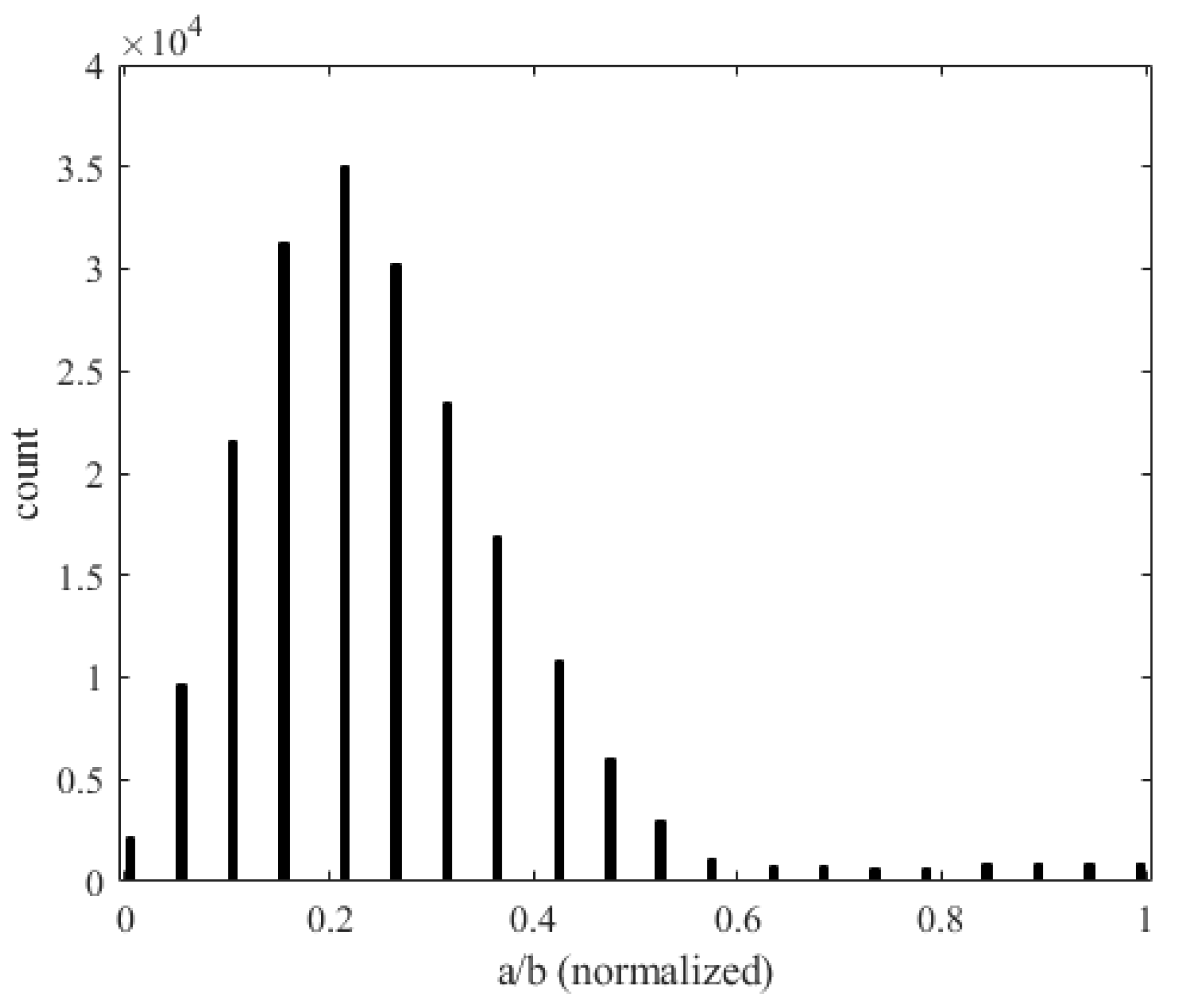
Solving the full-order model (Equation (19)) 707,472,000 times requires substantial computational effort, as it involves solving PDEs for each sample. This process is highly time-consuming, taking approximately 5.5 h on a CPU Intel i9-13900. Using CFD for grid points and fluid–solid coupling would significantly increase this time. In contrast, deep learning models are more efficient. Once trained, they can predict results for the entire dataset in less than 1 min, drastically reducing computational costs. To validate our deep neural network within aeroelasticity theory, we analyzed various flight conditions of small panels. After normalizing the input features, Figure 43 shows the relationship between panel aspect ratio (a/b) and flutter occurrences. The horizontal axis represents the aspect ratio and the vertical axis shows the number of flutter occurrences. Longer panels (greater a) better withstand deformation in the wind direction, absorbing energy from longitudinal forces and reducing flutter amplitude. Figure 44 shows the relationship between the air density (altitude) and the number of occurrences of flutter. The horizontal axis represents the normalized air density (altitude) and the vertical axis represents the number of flutter occurrences. As the altitude increases, the air density decreases, which reduces the aeroelastic impact on the panel, thereby reducing the occurrence of flutter.
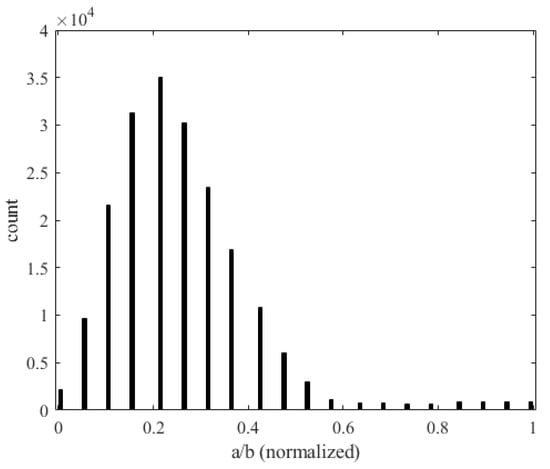
Figure 43.
Histogram of the aspect ratio (a/b) and occurrence of flutter.
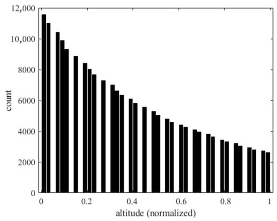
Figure 44.
Histogram of air density (altitude) and the occurrence of flutter.
Figure 45 shows the relationship between the frequency () of the panel and the number of occurrences of flutter. The horizontal axis represents the frequency and the vertical axis represents the number of flutter occurrences. As the vibration frequency increases, most of the energy is absorbed by the vibration frequency, thus reducing the amplitude of flutter and the occurrence of flutter.
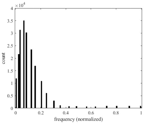
Figure 45.
Histogram of frequency and the occurrence of flutter.
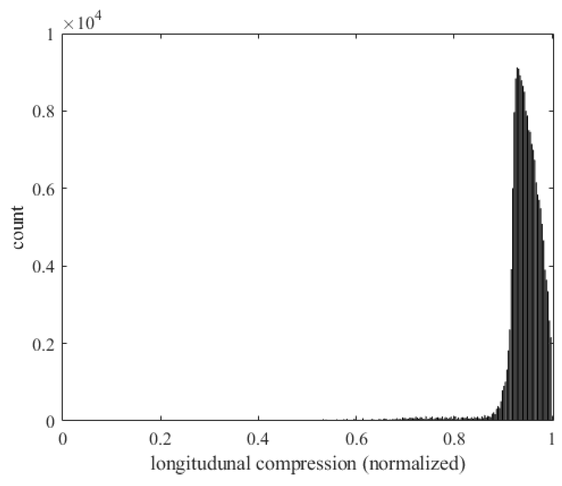
Figure 46 shows the relationship between the longitudinal compression () on the panel and the number of occurrences of flutter. The horizontal axis represents the longitudinal compression and the vertical axis represents the number of flutter occurrences. When the panel is subjected to a larger longitudinal force, the structure deforms more, making the panel more unstable and increasing the risk of flutter.
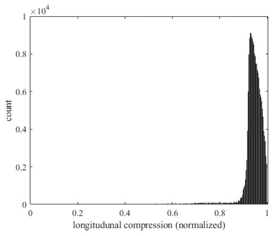
Figure 46.
Histogram of longitudinal force and the occurrence of flutter.
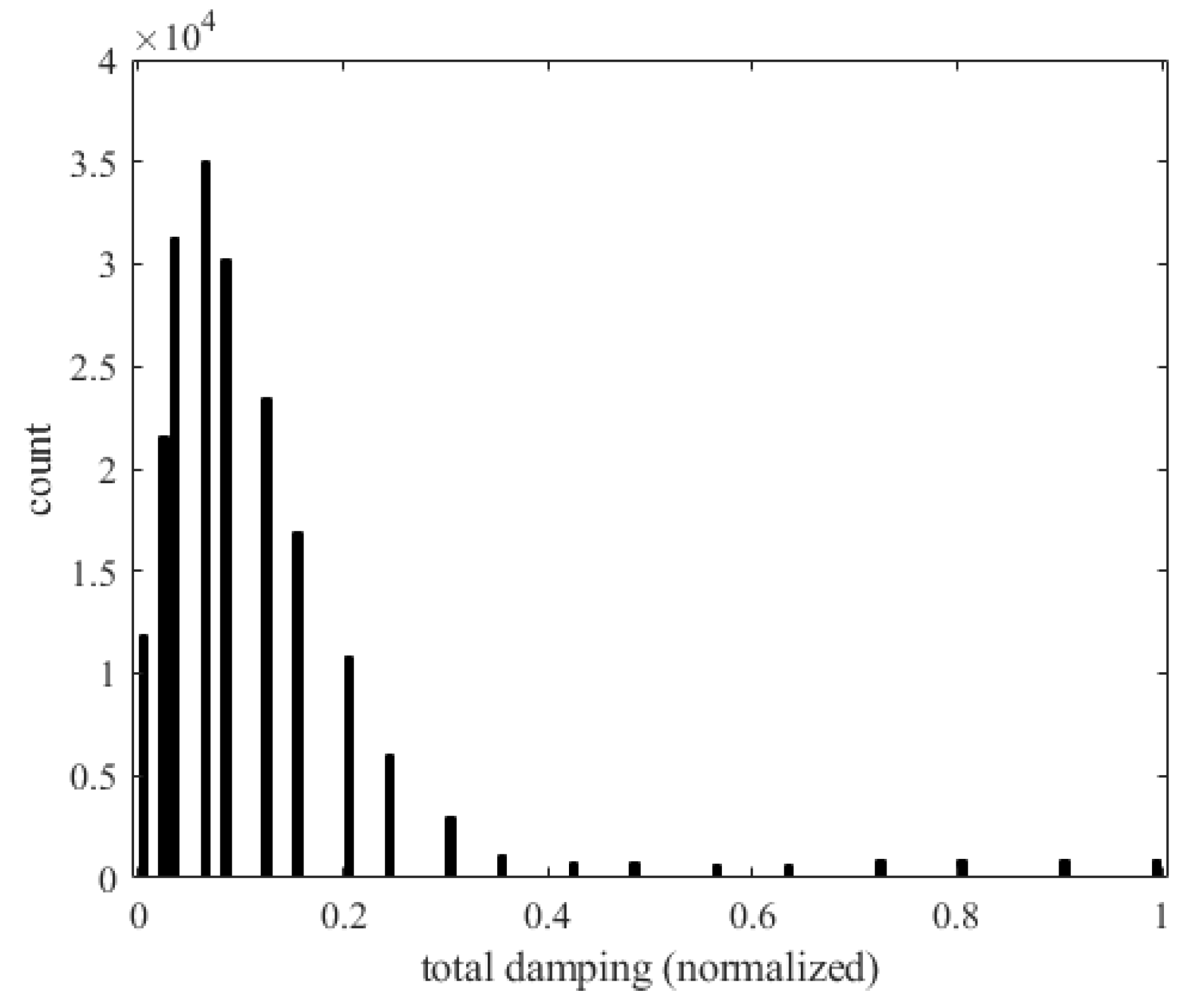
Figure 47 shows the relationship between the total damping (gT) of the panel and the number of occurrences of flutter. The horizontal axis represents the total damping and the vertical axis represents the number of flutter occurrences. As damping increases, vibration energy is rapidly dissipated. When the amplitude of the panel decreases, the interaction between aerodynamic forces and the structure weakens, reducing the risk of flutter.

Figure 47.
Histogram of total damping and the occurrence of flutter.
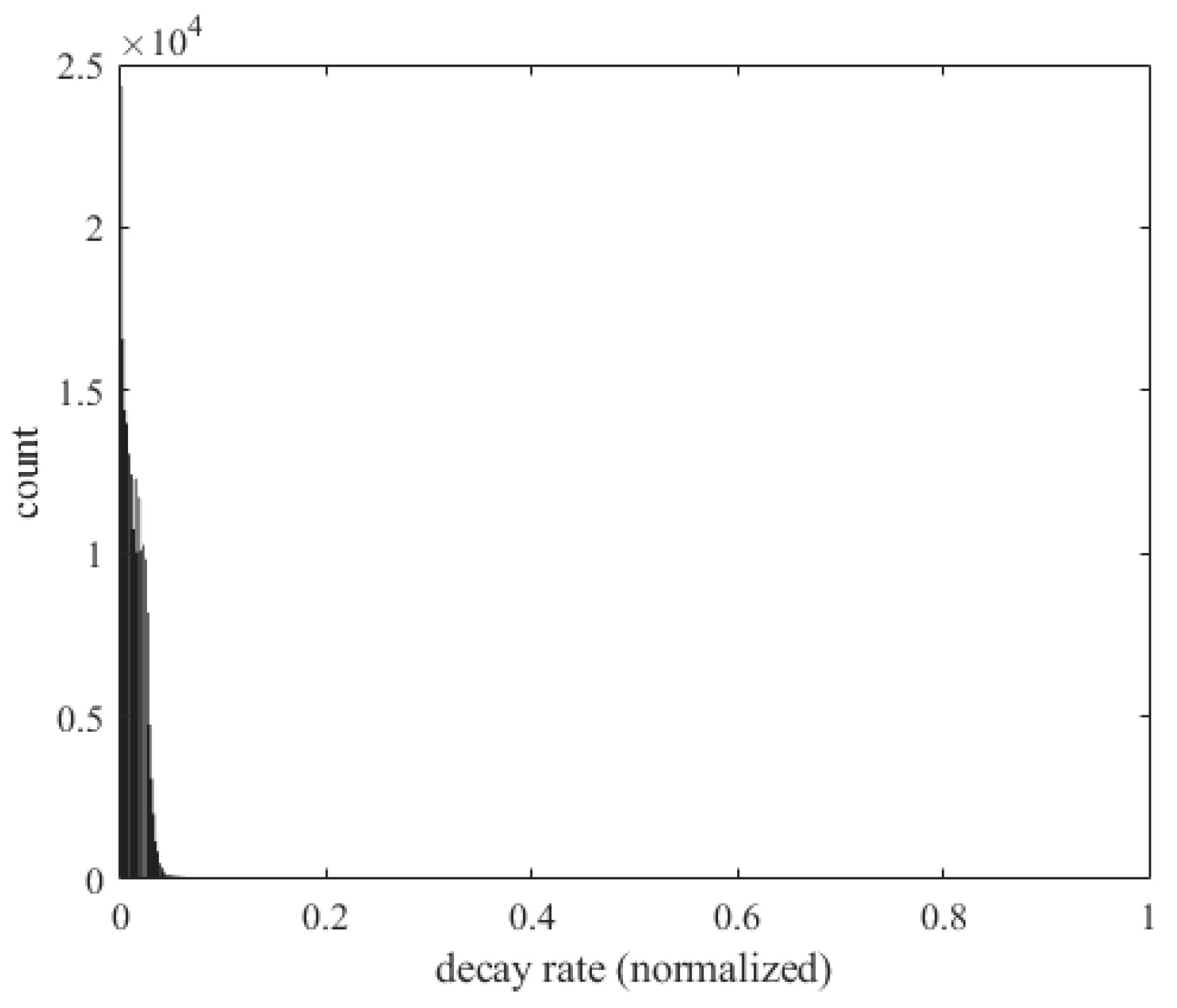
Figure 48 shows the decay rate () and the number of occurrences of flutter. The horizontal axis represents the decay rate and the vertical axis represents the number of flutter occurrences. A larger damping rate means that the vibration energy in the system dissipates faster. When the small plate is subjected to external disturbances, the vibration energy quickly decays, preventing the system from entering an unstable state.

Figure 48.
Histogram of the decay rate and occurrence of flutter.
Through these graphical explanations, we ensure that the data in this study align with physical principles, thereby confirming the reliability of the deep neural network models used in this research.
A description of the pros and cons of this method compared to modern numerical complex systems that allow very detailed coupled simulations is given as follows:
- Pros:
- Efficiency and Speed:
DL Models: Deep learning (DL) models offer significant computational efficiency and speed. Once trained, they can quickly predict panel flutter, making them suitable for real-time monitoring and design optimization applications.
Numerical Complex Systems: High-fidelity numerical simulations, such as CFD-FEM coupled systems, are computationally intensive and time-consuming, which can be a limitation for real-time applications;
- Scalability:
DL Models: DL models are highly scalable and can be trained on large datasets, as demonstrated in our study with over 700,000,000 data points. This scalability ensures robustness and generalizability to various flight conditions and panel configurations.
Numerical Complex Systems: These systems, while highly accurate, require substantial computational resources, limiting their scalability and practicality for extensive parameter studies or real-time applications;
- Predictive Accuracy:
DL Models: Our study demonstrates that DL models, particularly LSTM-NN, achieve high predictive accuracy in capturing flutter phenomena. The results in Figure 42, Figure 43, Figure 44, Figure 45, Figure 46 and Figure 47 are consistent with the physical phenomena of flutter, proving the sufficiency of our theoretical model in capturing conditions that constitute flutter.
Numerical Complex Systems: These systems provide highly accurate and detailed simulations, which are essential for critical design and safety assessments.
- Cons:
- Physical Insight:
DL Models: While DL models offer efficient predictions, they may lack the detailed physical insights that numerical simulations provide. This could potentially limit their explanatory power in understanding the underlying mechanisms of aeroelastic phenomena. However, it is important to note that the consistency of our results with known physical phenomena, as shown in Figure 42, Figure 43, Figure 44, Figure 45, Figure 46 and Figure 47, and the use of a typical panel plate aeroelastic equation (Reference [30]) demonstrate that our theoretical model is sufficient as a database for machine learning. This indicates that the perceived lack of physical insight is not necessarily a limitation in this context.
Numerical Complex Systems: High-fidelity simulations offer detailed insights into physical phenomena, aiding in a deeper understanding of the underlying mechanics and interactions. These insights are crucial for developing comprehensive and accurate aeroelastic models.
While deep learning models provide significant advantages in terms of computational efficiency, scalability, and predictive accuracy, high-fidelity numerical simulations offer unmatched physical insights. Our study bridges this gap by demonstrating that the theoretical model used is sufficient to capture the conditions leading to flutter, providing a robust database for machine learning. This hybrid approach leverages the strengths of both methodologies, ensuring efficient and accurate predictions while maintaining physical relevance.
We used the constitutive equations of a simply supported panel due to their simplicity and well-understood behavior, making them ideal for initial model validation. This approach allowed us to focus on the effectiveness of deep learning models without the added complexity of wing flutter equations. The results in Figure 42, Figure 43, Figure 44, Figure 45, Figure 46 and Figure 47 are consistent with physical flutter phenomena and validate the theoretical model. Reference [30] also supports the use of this typical aeroelastic equation, proving its adequacy for machine learning. Our study’s input features included the panel aspect ratio, Mach number, air density, and decay rate, which were chosen for their relevance to aeroelastic behavior. In our sensitivity analysis, the Mach number had the highest impact on model predictions, highlighting its crucial role in aeroelastic phenomena. The panel aspect ratio significantly affected model performance, altering structural dynamics and flutter characteristics. Air density showed a moderate impact, which was more pronounced in high-speed conditions. The decay rate had the least impact but influenced model fine-tuning.
The analysis underscores the importance of including the Mach number and panel aspect ratio, which are relevant to guiding feature selection and potentially reducing model complexity. The accurate prediction of panel flutter ensures the structural integrity of aircraft components, providing early warnings and reducing the need for extensive physical testing. Our models can explore a wider range of design parameters and flight conditions, enhancing design optimization and robustness. Applications extend to wind turbine blades, the automotive industry, and structures like bridges and tall buildings, predicting and mitigating aeroelastic instabilities to improve safety and performance.
5. Conclusions
This study primarily focuses on supersonic panels, incorporating various flight conditions into the aeroelastic equation to analyze and label structural vibration results, thus creating a large database. We used DNN, LSTM, and LSTM-NN models to predict the convergence, stability boundary, or divergence of the aeroelastic system and the Mach number for panel flutter. We compared the advantages and differences in these three deep learning models and validated the database’s accuracy using principles from aeroelastic mechanics and aerodynamics. The main conclusions of this study are as follows:
- (1)
- Data Preprocessing: Data preprocessing is crucial in this study. Without optimized preprocessing, the training results would be very poor. Therefore, before training the model, we normalized the features through feature scaling, ensuring the values’ magnitude does not affect the model weights. This also accelerates the model’s convergence, reducing training time;
- (2)
- Batch Size: In model architecture, the batch size determines the number of samples used to update model parameters in each iteration. Increasing the batch size often led to instability during training. Although smaller batch sizes result in slower training speeds, they tend to yield better accuracy and faster convergence;
- (3)
- Model Parameters: Whether using DNN, LSTM, or LSTM-NN, having too many hidden layers, epochs, and neurons without proper tuning can lead to overfitting. Selecting appropriate hidden layers, epochs, and neurons is essential to avoid such issues;
- (4)
- Neurons and Hidden Layers: More neurons and hidden layers can improve model training results, but beyond a certain point, they do not enhance accuracy and can cause overfitting. Therefore, selecting suitable neurons and hidden layers is critical for effective model training;
- (5)
- Model Comparison: In this study, the LSTM-NN model showed the highest accuracy in training, validation, and prediction compared to the DNN and LSTM models. For regression tasks involving flutter Mach number, the LSTM model performed best. The addition of neural network layers to LSTM models effectively extracted sequence features and improved classification accuracy. LSTM models excel at regression tasks due to their ability to capture long-term dependencies and complex nonlinear relationships;
- (6)
- Training Time: Although LSTM models achieve better accuracy in both classification and regression tasks, their computational complexity results in longer training times compared to DNN. Thus, there is a need to balance the accuracy improvements against the increased training time to select the most appropriate model.
For this research, Python and TensorFlow were used as the primary tools. Python, being easy to learn and feature-rich, provides a wide array of libraries and tools. TensorFlow, a powerful machine learning framework, offers rich and advanced APIs and built-in algorithms, supporting flexible and custom model architectures and training. By using deep learning, this study successfully developed models to predict panel motion states and flutter Mach numbers, both yielding satisfactory results. The findings indicate that deep learning is an effective method for prediction, showcasing its broad applications and significant potential in aerospace engineering.
Author Contributions
Conceptualization, Y.-R.W.; methodology, Y.-R.W. and Y.-H.M.; software, Y.-H.M.; validation, Y.-R.W.; formal analysis, Y.-R.W. and Y.-H.M.; investigation, Y.-R.W. and Y.-H.M.; resources, Y.-R.W.; writing—original draft preparation, Y.-R.W.; writing—review and editing, Y.-R.W. All authors have read and agreed to the published version of the manuscript.
Funding
This research was funded by the National Science and Technology Council, R.O.C., grant number NSTC 113-2221-E-032-011.
Data Availability Statement
Data are contained within the article.
Conflicts of Interest
The authors declare no conflicts of interest.
References
- Vedeneev, V.V.; Guvernyuk, S.V.; Zubkov, A.F.; Kolotnikov, M.E. Experimental observation of single mode panel flutter in supersonic gas flow. J. Fluids Struct. 2010, 26, 764–779. [Google Scholar] [CrossRef]
- Sun, G.; Wang, S. A review of the artificial neural network surrogate modeling in aerodynamic design. Proc. Inst. Mech. Eng. Part G J. Aerosp. Eng. 2019, 233, 5863–5872. [Google Scholar] [CrossRef]
- Teimourian, A.; Rohacs, D.; Dimililer, K.; Teimourian, H.; Yildiz, M.; Kale, U. Airfoil aerodynamic performance prediction using machine learning and surrogate modeling. Heliyon 2024, 10, E29377. [Google Scholar] [CrossRef]
- Antimirova, E.; Jung, J.; Zhang, Z.; Machuca, A.; Gu, G.X. Overview of Computational Methods to Predict Flutter in Aircraft. ASME. J. Appl. Mech. 2024, 91, 050801. [Google Scholar] [CrossRef]
- Li, W.; Gao, X.; Liu, H. Efficient prediction of transonic flutter boundaries for varying Mach number and angle of attack via LSTM network. Aerosp. Sci. Technol. 2021, 110, 106451. [Google Scholar] [CrossRef]
- Shubov, M.A. Flutter phenomenon in aeroelasticity and its mathematical analysis. J. Aerosp. Eng. 2006, 19, 1–12. [Google Scholar] [CrossRef]
- Fung, Y. On two-dimensional panel flutter. J. Aerosp. Sci. 1958, 25, 145–160. [Google Scholar] [CrossRef]
- Dinulović, M.; Benign, A.; Rašuo, B. Composite Fins Subsonic Flutter Prediction Based on Machine Learning. Aerospace 2024, 11, 26. [Google Scholar] [CrossRef]
- Najafabadi, M.M.; Villanustre, F.; Khoshgoftaar, T.M.; Seliya, N.; Wald, R.; Muharemagic, E. Deep learning applications and challenges in big data analytics. J. Big Data 2015, 2, 1. [Google Scholar] [CrossRef]
- Hao, K. We Analyzed 16,625 Papers to Figure out Where AI Is Headed Next. MIT Technology Review. 2019. Available online: https://www.technologyreview.com/2019/01/25/1436/we-analyzed-16625-papers-to-figure-out-where-ai-is-headed-next/ (accessed on 30 June 2024).
- Olston, C.; Fiedel, N.; Gorovoy, K.; Harmsen, J.; Lao, L.; Li, F.; Rajashekhar, V.; Ramesh, S.; Soyke, J. Tensorflow-serving: Flexible, high-performance ml serving. arXiv 2017, arXiv:1712.06139. [Google Scholar]
- Bisplinghoff, R.L.; Ashley, H. Principles of Aeroelasticity; Wiley: New York, NY, USA, 1975; pp. 161–181. [Google Scholar]
- Dowell, E.H.; Clark, R.A.; Cox, D.E.; Curtiss, H.C.; Edwards, J.W.; Hall, K.C. A Modern Course in Aeroelasticity; Springer Science + Business Media, Inc.: New York, NY, USA, 2005; pp. 651–658. [Google Scholar]
- Sayed, M.; Bucher, P.; Guma, G.; Lutz, T.; Wüchner, R. Aeroelastic Simulations Based on High-Fidelity CFD and CSD Models. In Handbook of Wind Energy Aerodynamics; Stoevesandt, B., Schepers, G., Fuglsang, P., Yuping, S., Eds.; Springer: Cham, Switzerland, 2021. [Google Scholar] [CrossRef]
- Lamorte, N.; Friedmann, P.P. Hypersonic Aeroelastic and Aerothermoelastic Studies Using Computational Fluid Dynamics. AIAA J. 2014, 52, 2062–2078. [Google Scholar] [CrossRef]
- Hinton, G.E.; Osindero, S.; Teh, Y.-W. A fast learning algorithm for deep belief nets. Neural Comput. 2006, 18, 1527–1554. [Google Scholar] [CrossRef]
- Srivastava, N.; Hinton, G.; Krizhevsky, A.; Sutskever, I.; Salakhutdinov, R. Dropout: A simple way to prevent neural networks from overfitting. J. Mach. Learn. Res. 2014, 15, 1929–1958. [Google Scholar]
- Kingma, D.P.; Ba, J. Adam: A method for stochastic optimization. arXiv 2014, arXiv:1412.6980. [Google Scholar]
- Rosenblatt, F. The perceptron: A probabilistic model for information storage and organization in the brain. Psychol. Rev. 1958, 65, 386. [Google Scholar] [CrossRef]
- Werbos, P. Backpropagation through time: What it does and how to do it. Proc. IEEE 1990, 78, 1550–1560. [Google Scholar] [CrossRef]
- Hopfield, J.J. Neural networks and physical systems with emergent collective computational abilities. Proc. Natl. Acad. Sci. USA 1982, 79, 2554–2558. [Google Scholar] [CrossRef]
- Hochreiter, S.; Schmidhuber, J. Long short-term memory. Neural Comput. 1997, 9, 1735–1780. [Google Scholar] [CrossRef]
- Ding, B.; Qian, H.; Zhou, J. Activation functions and their characteristics in deep neural networks. In Proceedings of the 2018 Chinese Control and Decision Conference (CCDC), Shenyang, China, 9–11 June 2018; pp. 1836–1841. Available online: https://api.semanticscholar.org/CorpusID:51601130 (accessed on 29 June 2024).
- Keskar, N.S.; Mudigere, D.; Nocedal, J.; Smelyanskiy, M.; Tang, P.T.P. On large-batch training for deep learning: Generalization gap and sharp minima. arXiv 2016, arXiv:1609.04836. [Google Scholar]
- Solgi, R.; Loaiciga, H.A.; Kram, M. Long short-term memory neural network (LSTM-NN) for aquifer level time series forecasting using in-situ piezometric observations. J. Hydrol. 2021, 601, 126800. [Google Scholar] [CrossRef]
- Liao, H.; Mei, H.; Hu, G.; Wu, B.; Wang, Q. Machine learning strategy for predicting flutter performance of streamlined box girders. J. Wind. Eng. Ind. Aerodyn. 2021, 209, 104493. [Google Scholar] [CrossRef]
- Sabater, C.; Stürmer, P.; Bekemeyer, P. Fast predictions of aircraft aerodynamics using deep-learning techniques. AIAA J. 2022, 60, 5249–5261. [Google Scholar] [CrossRef]
- Baykal, S.I.; Bulut, D.; Sahingoz, O.K. Comparing deep learning performance on BigData by using CPUs and GPUs. In Proceedings of the 2018 Electric Electronics, Computer Science, Biomedical Engineerings’ Meeting (EBBT), Istanbul, Turkey, 18–19 April 2018; pp. 1–6. [Google Scholar] [CrossRef]
- Buber, E.; Banu, D. Performance analysis and CPU vs GPU comparison for deep learning. In Proceedings of the 2018 6th International Conference on Control Engineering & Information Technology (CEIT), Istanbul, Turkey, 25–27 October 2018; pp. 1–6. [Google Scholar] [CrossRef]
- Dugundji, J. Theoretical considerations of panel flutter at high supersonic Mach numbers. AIAA J. 1966, 4, 1257–1266. [Google Scholar] [CrossRef]
- Mahesh, B. Machine learning algorithms—A review. Int. J. Sci. Res. 2020, 9, 381–386. [Google Scholar] [CrossRef]
- LeCun, Y.; Bengio, Y.; Hinton, G. Deep learning. Nature 2015, 521, 436–444. [Google Scholar] [CrossRef]
- Montavon, G.; Samek, W.; Müller, K.R. Methods for interpreting and understanding deep neural networks. Digit. Signal Process. 2018, 73, 1–15. [Google Scholar] [CrossRef]
Disclaimer/Publisher’s Note: The statements, opinions and data contained in all publications are solely those of the individual author(s) and contributor(s) and not of MDPI and/or the editor(s). MDPI and/or the editor(s) disclaim responsibility for any injury to people or property resulting from any ideas, methods, instructions or products referred to in the content. |
© 2024 by the authors. Licensee MDPI, Basel, Switzerland. This article is an open access article distributed under the terms and conditions of the Creative Commons Attribution (CC BY) license (https://creativecommons.org/licenses/by/4.0/).

