Advanced UAV Design Optimization Through Deep Learning-Based Surrogate Models

Abstract

The conceptual design of unmanned aerial vehicles (UAVs) presents significant multidisciplinary challenges requiring the optimization of aerodynamic and structural performance, stealth, and propulsion efficiency. This work addresses these challenges by integrating deep neural networks with a multiobjective genetic algorithm to optimize UAV configurations. The proposed framework enables a comprehensive evaluation of design alternatives by estimating key performance metrics required for different operational requirements. The design process resulted in a significant improvement in computational time over traditional methods by more than three orders of magnitude. The findings illustrate the framework’s capability to optimize UAV designs for a variety of mission scenarios, including specialized tasks such as intelligence, surveillance, and reconnaissance (ISR), combat air patrol (CAP), and Suppression of Enemy Air Defenses (SEAD). This flexibility and adaptability was demonstrated through a case study, showcasing the method’s effectiveness in tailoring UAV configurations to meet specific operational requirements while balancing trade-offs between aerodynamic efficiency, stealth, and structural weight. Additionally, these results underscore the transformative impact of integrating AI into the early stages of the design process, facilitating rapid prototyping and innovation in aerospace engineering. Consequently, the current work demonstrates the potential of AI-driven optimization to revolutionize UAV design by providing a robust and effective tool for solving complex engineering problems.

1. Introduction

The aircraft design process is a procedure that has evolved over almost a century, covering gradual phases that are both time- and cost-intensive and result in the production of highly complex products. While witnessing advancements in various facets of the design process, the standardization of the process into a specific framework has been largely shaped by the developments in computational engineering in recent decades. When considering unconventional concepts and operational requirements, especially in the realm of unmanned aerial vehicles, it becomes apparent that the traditional design process may lack the necessary flexibility and hinder the exploration of the design space. In this context, machine learning techniques, which have gained popularity in the last decade due to increased accessibility to high computational power, have the potential to enhance creativity in design methodology.

1.1. Overview of Aircraft Design

A review of the historical evolution of aircraft design processes reveals that the first vehicles were developed through experimental and trial-and-error approaches. During the World Wars era, the notable advances in aerospace engineering led to a clear differentiation of subdisciplines within the design process. In parallel with the Jet Age, the evolution of computers has brought about a revolutionary change in the aircraft design procedure, notably through the implementation of computer-aided design (CAD) and computational analysis methods. These technologies have enabled engineers to develop intricate and precise digital models, conduct sophisticated simulations, and perform analyses with enhanced accuracy and efficiency. In this way, the dependence on the wind tunnel was reduced, opening the way for easier and faster iterative design [1]. At the same time, developments in these tools and differences in fidelity in analysis methodologies have led to a more systematic approach to the design process. The design process was structured into three fundamental phases, spanning from initial requirements to the prototyping and manufacturing stage: conceptual design, preliminary design, and detailed design.

The first and crucial stage of the design process is the conceptual design phase, where the aircraft is defined at the system level. During this phase, multiple concepts are analyzed, and the selected design is the one that most effectively meets the mission requirements. The complications involved in the aircraft design process require a systematic approach that involves decomposition using a hierarchical structure of various levels. As the design process progresses from one phase to the next, there is a significant increase in the fidelity of the product, the complexity of the model, and the time required for completion. The conceptual design stage is highly critical, with many decisions made under significant uncertainty, and actual costs are revealed much later in the process [2]. However, the level of human interaction in this process is quite intensive. As seen in Figure 1, changes are easier to implement in the early stages of design, while the commitment to the configuration is at its lowest. As the process progresses, these two phenomena change in opposite proportions. However, the most critical point here is that the change in design can result in very high costs in the later stages. Therefore, it is important to determine the correct configuration by minimizing human interaction in the early stages. In the classical approach, fast but low-level approaches, such as historical data, semi-empirical methods, and figure of merit (FoM), are preferred to aid configuration selection [3,4,5]. The potential for innovation is highest in the early design process, making it imperative to increase fidelity during the initial design stages to minimize uncertainty [6]. This poses a problem in the design of complex, innovative, and unconventional vehicles.

By its very nature, aircraft design is an iterative process. When aircraft design procedures are examined, various flowcharts on this subject can be found [7]. However, the primary issue here is that this process is highly human-centric in nature at present. This issue particularly comes to the fore in the initial layout/concept sketch phase. Upon analysis of the design processes during the conceptual and early preliminary design stages, it becomes apparent that the conceptual phase drives configuration design, while the preliminary design phase focuses on component design and sizing. Methods such as topology optimization that will provide these two simultaneously are quite difficult for aircraft geometries, as the limited design points are insufficient to represent the entire geometry [8]. Therefore, a new approach is needed that incorporates primarily the sizing of components and the selection of configurations.

1.2. Design from the Perspective of Unmanned Aerial Vehicles

The design procedure, particularly in the case of unmanned aerial vehicles, involves certain differences. Specifically, when concepts of unmanned aerial vehicles are addressed, all considerations and constraints related to pilots and crew are removed. In today’s context, the autonomous control systems, material technologies, and new production techniques used in these vehicles drive the design process to move in a different direction. If operational requirements are taken into account, the situation becomes even more complex. This complexity arises from the need to maximize operational efficiency, minimize risks, and meet diverse mission requirements while adapting to advances in technology and market demands. In this sense, systems that utilize common components and enable rapid and cost-effective production are at the forefront.

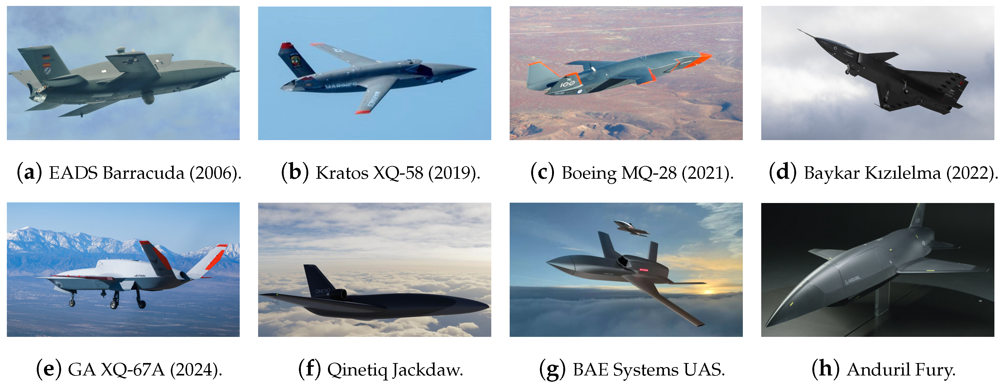
Especially when considering an autonomous system, it is no longer possible to approach these vehicles as conventional aerial vehicles as they are increasingly viewed as high-tech systems/robots. The concept that technological tools can be shaped according to humanity’s interests and thus possess disposable features has been explored in various science-fiction works [9]. The aforementioned systems, which can be compared to the swarms of robotic machines depicted as off-world technology in twentieth-century works, have quickly become an inevitable reality in today’s complex tactical environment [10]. Such systems, which are mass-produced in large numbers, are considered attritable because of their low life-cycle cost (LCC) expectancy. This compels the design process to move towards cost-effectiveness as much as possible. Figure 2 illustrates various prototypes and concepts of “attritable/reusable” and “loyal/robotic wingman” UAVs developed within the manned–unmanned teaming (MUM-T) framework. These vehicles stand out from existing tactical UAV systems due to their high subsonic cruise speeds, high maneuverability, and limited stealth capabilities. Additionally, unlike blended wing body concept stealth UAVs, which have much higher maximum takeoff weights (MTOWs) and costs, these prototypes offer limited payload capacities but affordable life-cycle costs. A key challenge lies in developing design approaches that incorporate nonconventional perspectives, particularly in the next-generation design of “plug and play” configurations across a fleet of unmanned combat aerial vehicles (UCAVs) [11,12,13]. These vehicles are expected to fulfill a variety of different mission requirements while minimizing entire life-cycle costs [14,15,16,17,18,19]. For instance, an ISR (intelligence, surveillance, and reconnaissance) mission requires high endurance and various payloads for observation, while an EW (electronic warfare) mission demands high range and cruising speed. A SEAD (Suppression of Enemy Air Defenses) mission additionally requires high maneuverability and a low radar cross section (RCS). All of these operations can be performed by changing the modular lifting surfaces (wing, tail, or canard) and/or fuselage components of a single configuration. Selecting the most appropriate components for each mission scenario requires navigating through numerous optimal points within a huge design space.

As in the case mentioned, the design process often requires the integration of multiple engineering disciplines. The multidisciplinary design optimization (MDO) approach consolidates all disciplines into a unified framework. MDO refers to the design of complex engineering systems comprising interactive subsystems influenced by interdependent physical phenomena [28]. In aircraft design studies, typical disciplines within MDO include aerodynamics, structures, weight and balance, and propulsion. As indicated in [29], aircraft design optimization has historically utilized semi-empirical equations to rapidly analyze conventional fixed-wing aircraft. However, applying these low-fidelity models to UAVs can pose challenges due to their reliance on traditional fixed-wing regression data. In general, the data in semi-empirical approaches are not very accurate, especially in terms of aerodynamic performance, as stated in [30], since they do not cover the dimensions and flight conditions of UAVs. Therefore, more complex approaches, such as numerical methods, should enter the design process earlier. However, performing optimization through high-fidelity tools, which require many evaluations of the mathematical model to compute the performance of the system at each iteration loop, can be computationally expensive and time-consuming [31]. At this point, machine learning-based solutions come to the fore in the literature as an alternative approach to this problem.

1.3. Design Solutions Using Machine Learning

Machine learning is a computational approach that enables systems to learn and improve from experience without explicitly programming them, with a primary focus on exploiting data to improve performance and make informed decisions. The field of aerospace engineering, which is packed with data and already constructed on a limited multiobjective optimization framework that is perfectly suited for contemporary machine learning approaches, is perhaps the best example of the potential for data-driven advancement [32]. In particular, in terms of design optimization and upgrade analysis, performance validation and optimization, and product improvement and calibration, machine learning-based digital twins offer significant advantages [33].

In the literature, various studies have been conducted that utilize machine learning to address the design problems of aerial vehicles. In [34], the research explores the selection of configurations using a database of existing UAVs through the application of decision tree classifiers. Sharma and Hosder [35] investigated the feasibility of using neural network models to predict the maximum take-off weight, fuselage length, thrust, and aspect ratio of airliner configurations. In terms of the design point, Oroumieh et al. [36] introduced an approach using fuzzy logic and neural networks to determine the wing area and engine thrust and validated this approach through an application to a specific class of light business jets. In the study conducted by Boutemedjet et al. [37] for the design of small UAVs, the design parameters were statistically derived from historical trends of existing UAVs, and the wing planform was optimized using a neural network-based aerodynamic model. In [38], a meta-model of the multidisciplinary design and analysis module with neural networks was developed and used to obtain the handling qualities of a small UAV.

In addition, machine learning algorithms have become widely used in aerodynamic design and design optimization as surrogate models. Bekemeyer et al. [39] developed a surrogate modeling toolbox utilizing data-driven techniques such as deep learning, data fusion, and reduced-order modeling to meet the comprehensive requirements of aerodynamic data for design and certification processes. In [40], Sharma and Hosder examine the feasibility of using machine learning models, specifically artificial neural networks, to predict aircraft configuration design variables from mission-informed performance data for blended wing body aircraft, showing that such models significantly improve prediction accuracy and computational efficiency. Wu et al. [41], addressing the missile design optimization problem, developed an algorithm that utilizes a convolutional neural network (CNN) for feature extraction from design drawings and a multitask learning-based neural network model to predict aerodynamic parameters such as axial force, normal force, pitching moment, and pressure center, thereby accelerating the design process. Yan et al. [42] developed an algorithm for aerodynamic shape optimization of missile control surfaces, employing reinforcement learning for extracting optimization experience from DATCOM and transfer learning for CFD-based optimization, significantly reducing computational costs and accelerating the design process by over 62.5%. Furthermore, Li et al. [43] provided a comprehensive review of machine learning applications in aerodynamic shape optimization and summarized some of the successful algorithms and applications in compact geometric design space, fast aerodynamic analysis, and efficient optimization architecture. In [44,45,46,47,48,49,50,51], artificial neural networks and convolutional neural network algorithms were used to predict the aerodynamic performance of various components of the aircraft, such as the airfoil, the nacelle of the engine, and the wing. Furthermore, comparisons between models based on artificial intelligence and classical methods have demonstrated significant advantages for AI as data sets expand [52]. Traditional methods reliant on statistical approaches tend to become redundant, overshadowed by the substantial reductions in computation time offered by AI techniques, which often show order-of-magnitude improvements. Furthermore, the authors have discovered that machine learning techniques, in particular neural networks, have great potential in these areas. In [30], we developed deep learning-based surrogate models to capture the nonlinear aerodynamic performance of conventional small UAV configurations. In [53], we developed a neural network-based deep transfer learning model with a multifidelity approach to predict the aerodynamic performance of next-generation low-cost modular UCAVs. These AI models leverage advanced machine learning algorithms to process and analyze large volumes of data more efficiently than classical methods. Consequently, AI-driven optimizations in fields like aerospace and engineering are not only faster but also promise to deliver more innovative and effective solutions. The scalability of AI methods enables them to handle complex, multivariable problems with greater precision, retaining the potential to significantly accelerate the development cycles of new technologies.

The remainder of this paper is organized as follows. Section 2 outlines the conceptual framework and highlights the novelty of the developed algorithm, which integrates mission requirements with geometry design through multidisciplinary approaches and AI-driven models. Section 3 details the methodology, starting with the initial sizing algorithm that employs fundamental flight performance equations to establish baseline dimensions and metrics for the UAV. Following, the aircraft model is explained in detail under the topics of aerodynamics, radar cross section, structures, propulsion, and weights. In the rest of the section, mathematical and physical information about artificial neural network modeling and multiobjective genetic algorithms is given. Section 4 discussed the application of the model in an example case, demonstrating its practical utility. In Section 5, the results derived from the application scenario are presented, leading to Section 6, where conclusions are drawn from the findings and potential avenues for future research are suggested.

2. Conceptual Framework

In light of all this information, there has been an observed need to automate the current design process to incorporate more information at the early stages of design. The idea of developing a trustworthy intelligent algorithm that will link geometry design with mission requirements has emerged. In [54], we introduced a basic AI-driven framework that utilizes machine learning to enhance the configuration selection process in aircraft design. This algorithm, which initially considers only aerodynamics and structural performance parameters as part of the vehicle model, features an AI-supported optimization methodology. It identifies the best configuration from predefined concepts (conventional, lambda, and delta) based on specific mission criteria and establishes the initial layout. In [55], we explored a multidisciplinary conceptual design framework for UAVs that employs AI-driven surrogate models. This approach significantly improves the initial design stage, enabling the initial sizing of critical components and selection of the optimal configuration based on aerodynamics, structural mass, and radar cross-section predictions. These frameworks aim to streamline the design process, reduce costs, and enhance time efficiency by integrating multiple engineering disciplines and leveraging machine learning technologies.

In this work, a comprehensive structure is proposed based on previous experiences. The main goal is to establish an intelligent design algorithm that will match the given task with the optimum point in the design space. For this purpose, multipurpose, hierarchical, mixed-variable design spaces are efficiently explored with multidisciplinary design optimization located at the core, as given in Figure 3. Mission-level planning at the top of this structure defines operational standards and reduces mission-specific requirements to mission performance parameters. These parameters are used as objective functions and equality/inequality constraints in the optimization definition. At the base of the structure are surrogate models/digital twins to reduce the need for high-quality simulations across various disciplines. This layer, containing aerodynamics, structural, radar cross-section, weights, and propulsion models that may be required for an early-stage aircraft, allows instant estimation of performance parameters related to the vehicle at each point in the design space in the optimization cycle. To achieve this, in this work, a state-of-the-art physics-informed feature engineering approach is also developed. This study offers several key contributions to the field of UAV design optimization, which can be summarized as follows:

• Combines DNNs with multiobjective genetic algorithms for rapid UAV design optimization, speeding up the process by over three orders of magnitude.
• Develops a multidisciplinary framework integrating aerodynamics, structural analysis, radar cross section, and propulsion for comprehensive UAV evaluation.
• Utilizes physics-informed feature engineering for accurate surrogate models, predicting key UAV metrics with high precision.
• Optimizes UAV designs for specific missions by addressing distinct operational needs.

3. Methodology

This section presents a robust framework that employs a combination of mathematical modeling and computational simulations to optimize the design of unmanned aerial vehicles. The methodology starts with the design/mission requirements inputs, as shown in the flowchart in Figure 4, and is completed with the design of the optimum aerial vehicle configuration in accordance with these requirements.

The requirements given in the first stage are turned into design parameters with the initial sizing algorithm based on flight performance and design point calculations. Afterward, the most suitable design point is searched via multiobjective optimization within this determined design space. In this part, the design space is effectively searched by using AI-based vehicle models. These models are obtained by combining various disciplines with a framework that includes analysis, data generation, and training. The following sections detail the specific algorithms and computational models used and summarize their contribution to the design process.

3.1. Initial Sizing Algorithm

The initial sizing algorithm transforms the design requirements into design parameters. These requirements are provided as a list or mission profile. In a typical mission profile, as illustrated in Figure 5, there may be various targeted performance parameters and configurations for each flight phase. Therefore, it is crucial to identify a feasible design point area that simultaneously satisfies all these requirements.

In the calculation of design points, performance requirements such as stall speed $\left(V_{\mathrm{s}}\right)$, maximum speed $\left(V_{max}\right)$, maximum rate of climb $\left({\mathrm{ROC}}_{max}\right)$, take-off run $\left(S_{\mathrm{TO}}\right)$, and ceiling $\left(h_{\mathrm{c}}\right)$ are employed to determine a feasible design space in terms of wing loading ($W/S$) and thrust loading ($T/W$). Each of these parameters plays a crucial role in defining the design space and ensuring the UAV meets its intended operational capabilities:

• Stall speed $\left(V_{\mathrm{s}}\right)$: minimum speed for maintaining level flight.
• Maximum speed $\left(V_{max}\right)$: highest achievable speed in level flight.
• Rate of climb $\left({\mathrm{ROC}}_{max}\right)$: defines how quickly an aircraft gains height.
• Take-off run distance $\left(S_{\mathrm{TO}}\right)$: distance required for take-off.
• Ceiling altitude $\left(h_{\mathrm{c}}\right)$: maximum altitude for sustained level flight.

In order to identify the optimal selection, the flight performance equations are solved based on wing loading and thrust loading, and inequality constraints are generated accordingly. This method is entirely based on aircraft performance requirements and employs flight mechanics theory. Consequently, the procedure is analytical and yields highly reliable results.

The wing loading based on the stall speed requirements is shown as

$${\left({\displaystyle \frac{W}{S}}\right)}_{V_{\mathrm{s}}}={\displaystyle \frac{1}{2}}\rho V_{\mathrm{s}}^2{C}_{L_{max}}$$

(1)

where $\rho$ denotes the air density and $C_{L_{max}}$ is the maximum lift coefficient. The following relation is used for the maximum speed requirement:

$${\left({\displaystyle \frac{T_{\mathrm{SL}}}{W}}\right)}_{V_{max}}={\rho }_{\mathrm{o}}{V}_{max}^2{C}_{D_{\mathrm{o}}}{\displaystyle \frac{1}{2\left(\frac{W}{S}\right)}}+{\displaystyle \frac{2K}{\rho \sigma V_{max}^2}}\left({\displaystyle \frac{W}{S}}\right)$$

(2)

where ${\rho }_{\mathrm{o}}$ is the sea-level air density, $C_{D_{\mathrm{o}}}$ is the zero-lift drag coefficient, and K is referred to as the induced drag factor.

$${\left({\displaystyle \frac{T}{W}}\right)}_{S_{\mathrm{TO}}}={\displaystyle \frac{\mu -\left(\mu +\frac{C_{D_{\mathrm{G}}}}{C_{L_{\mathrm{R}}}}\right)\left[exp\left(0.6\rho g{C}_{D_{\mathrm{G}}}{S}_{\mathrm{TO}}\frac{1}{W/S}\right)\right]}{1-exp\left(0.6\rho g{C}_{D_{\mathrm{G}}}{S}_{\mathrm{TO}}\frac{1}{W/S}\right)}}$$

(3)

where $\mu$ is the friction coefficient of the runway surface and is generally taken as 0.05 for concrete/asphalt surfaces. $C_{L_{\mathrm{R}}}$ represents the aircraft lift coefficient in take-off rotation. It can be obtained by solving the lift equation inversely using take-off rotation speed $\left(1.1-1.2V_{\mathrm{s}}\right)$. $C_{D_{\mathrm{G}}}$ indicates the drag coefficient, accounting for ground effects during takeoff. The wing and engine sizing based on rate of climb requirements can be defined as follows:

$${\left({\displaystyle \frac{T}{W}}\right)}_{\mathrm{ROC}}={\displaystyle \frac{\mathrm{ROC}}{\sqrt{\frac{2}{\rho \sqrt{\frac{C_{D_0}}{K}}}\left(\frac{W}{S}\right)}}}+{\displaystyle \frac{1}{{(L/D)}_{max}}}$$

(4)

The ceiling is defined as the highest altitude at which an aircraft maintains its level flight. The ceiling is not a critical requirement for many aircraft, but it is critical for some missions, such as ISR (intelligence, surveillance, and reconnaissance). Similarly, as a function of wing and thrust loading, the performance equation can be stated as follows:

$${\left({\displaystyle \frac{T}{W}}\right)}_{h_{\mathrm{C}}}={\displaystyle \frac{{ROC}_C}{{\sigma }_{\mathrm{C}}\sqrt{\frac{2}{{\rho }_{\mathrm{C}}\sqrt{\frac{C_{D_{\mathrm{o}}}}{K}}}\left(\frac{W}{S}\right)}}}+{\displaystyle \frac{1}{{\sigma }_{\mathrm{C}}{(L/D)}_{max}}}$$

(5)

where ${\sigma }_{\mathrm{C}}$ is the relative air density and ${\rho }_{\mathrm{c}}$ is the air density, both at the ceiling altitude. The relevant equations can be found in aircraft design or flight performance textbooks [5,56]. In the initial design iteration, table-based aerodynamic and geometric data are used for unknown parameters. However, during subsequent design iterations, this information is directly derived from the aerodynamic performance and geometry of the previous configuration.

In the initial sizing phase, the fundamental dimensions of the aircraft are established based on the design point output and specific requirements. The wing area is derived by dividing the maximum take-off weight by the wing loading. Likewise, engine thrust is determined by multiplying the maximum take-off weight by the thrust loading. Through this process, the necessary wing area and engine thrust are calculated as follows:

$$S=W_{\mathrm{mtow}}/\left({\displaystyle \frac{W}{S}}\right),T=W_{\mathrm{mtow}}·\left({\displaystyle \frac{T}{W}}\right)$$

(6)

The selection of an engine is typically made from among existing engines, as developing a UAV-specific engine is not usually the first choice due to the constraints of cost and time. In addition to numerical evaluations, the selection of an engine is also influenced by factors such as the manufacturing country, production maintenance competence, usage permit, etc. Furthermore, the selection of an engine may also take into account factors such as specific fuel consumption and cost. Consequently, the current algorithm enables the user to select an engine that meets the required thrust level.

Table 1. Sample engine table for high subsonic UAV case [57,58,59,60,61,62,63,64,65,66].

Engine	Length (mm)	Diameter (mm)	Dry Weight (kg)	Maximum Thrust (kN)
Pratt Whitney Canada PW610F	1153	704	115.7	4.22
Pratt Whitney Canada PW615F	1258	750	140	6.49
Williams FJ33	976	466	140	8.21
Pratt Whitney Canada PW617	1360	750	172	8.41
GE Honda HF120	1510	660	211.3	9.10
Pratt Whitney Canada JT15D	1531	685.8	285.7	13.57
Honeywell TFE731-2	1844	1041	184	15.57
Williams FJ44-4	1340	640	298	16.00
Ivchenko AI-25TL	1494	611.6	350	16.90
Pratt Whitney Canada 545B	1742	693.4	376.5	17.58

lists some of the available turbofan engines that are suitable for high subsonic UAVs.

As illustrated in Figure 6, the fuselage is divided into three sections to determine the basic dimensions. In the case of the fore body, the sensor and avionics systems act as constraints. The dimensions of the mid-body are calculated based on the internal payload requirements. The length and diameter resulting from the selection of the engine are employed for the sizing of the aft body. All of these data are then utilized to determine a representative body length and hydraulic diameter.

3.2. Aircraft Model

This section provides a comprehensive review of the aircraft model and includes details on integrated disciplines. All these disciplines are created with mathematical and physical algorithms that allow for analysis of the aircraft from various aspects. First, the aerodynamic model analyzes airflow interactions and their impact on aircraft performance and calculates aerodynamic forces using computational aerodynamics methods. Following this, the radar cross section is assessed, focusing on the UAV’s detectability by radar through simulations that consider the shape of the aircraft. The structure model addresses the structural integrity and weight optimization of the UAV, utilizing finite element analysis (FEA) to ensure durability under aerodynamic loads. The propulsion model performs calculations related to the engine performance. Lastly, the weights model methodically calculates the distribution of weights, taking into account all the contributions of the previous subsystems.

3.2.1. Aerodynamics

An understanding of the aerodynamics of UAVs is of paramount importance to achieve optimal performance, efficiency, and mission success. It is crucial to determine the basic aerodynamic characteristics in the conceptual and preliminary design stages to ensure the successful development of UAVs. The initial stages of the development process involve pivotal decisions that have a significant impact on the entire process. By conducting an early assessment of aerodynamic characteristics, designers can make informed decisions about wing configurations, airfoil selections, and the overall vehicle layout.

In light of the necessity to analyze diverse geometries under specific flow conditions during the design stages, the deployment of rapid and precise aerodynamic solvers is of vital importance. Computational aerodynamic tools are typically classified into two categories: low- and high-fidelity methods. Low-fidelity methods, which simplify assumptions about flow equations, can calculate the forces and moments of basic components of aerial vehicles in seconds on a simple personal computer [67]. Examples of these methods include semi-empirical and potential theory-based approaches. In contrast, high-fidelity methods refer to CFD techniques that solve the complete Navier–Stokes equations for complex and detailed geometries. Table 2 compares different computational aerodynamic methods and notes their accuracy values as reported by [1].

Among low-order methods, potential flow-based panel methods offer more complex geometry modeling and solutions than semi-empirical methods and vortex lattice methods (VLM). However, panel methods remain less comprehensive than CFD solutions. Because panel methods use simplified forms derived from the Navier–Stokes equations, they ignore viscous effects and heat transfer, which means that they cannot compute skin friction drag, separation, or transonic shocks [68]. Despite this, panel methods have advantages over VLM, as they can model blunt geometries and apply boundary conditions on the actual surface rather than an average mean surface.

Table 2. Comparison of computational aerodynamic methods [69].

Approach	Primary Use	Accuracy (Average)	Computation Time	Examples
Semi-empirical methods	Conceptual design	$\pm 15\%$	Seconds on a PC	DATCOM, ESDU, AAA, RDS, etc.
Potential flow methods	Preliminary design	$\pm 10\%$	Seconds/minutes on a PC	VSPAero, PANAir, AVL, XFOIL, etc.
CFD methods	Detailed design	$\pm 5\%$	Hours/days/weeks on a WS/HPC	SU2, Fluent, USM3D, OpenFOAM, etc.

Table 2. Comparison of computational aerodynamic methods [69].

Approach	Primary Use	Accuracy (Average)	Computation Time	Examples
Semi-empirical methods	Conceptual design	$\pm 15\%$	Seconds on a PC	DATCOM, ESDU, AAA, RDS, etc.
Potential flow methods	Preliminary design	$\pm 10\%$	Seconds/minutes on a PC	VSPAero, PANAir, AVL, XFOIL, etc.
CFD methods	Detailed design	$\pm 5\%$	Hours/days/weeks on a WS/HPC	SU2, Fluent, USM3D, OpenFOAM, etc.

Panel methods can be briefly described as numerical schemes used to solve the linear, inviscid, irrotational flow equation at subsonic or supersonic free-stream Mach numbers. The name of the equation that the panel codes solve is the Prandtl–Glauert equation. For steady subsonic flow, this equation can usually be defined as

$${\tilde{\nabla }}^2\varphi =\left(1-M_{\infty }^2\right){\varphi }_{xx}+{\varphi }_{yy}+{\varphi }_{zz}=0$$

(7)

For subsonic flows, Equation (7) is elliptical. This type of equation allows any disturbance to be felt everywhere in the flow field, although the effect usually disappears with distance. To model the effect of geometry on flow, the singularities are distributed over the entire geometry and their strengths are calculated over the surface velocity boundary conditions. The velocities induced by each ring vortex at a specified control point are calculated using the Biot–Savart law. The contribution of each vortex loop and trailing wake at a given i control point is calculated as follows:

$${\overrightarrow{V}}_i=\sum _j^{\mathrm{Loops}}{\left[{\overrightarrow{V}}_{\mathrm{loop}}\right]}_j+\sum _j^{\mathrm{Wakes}}{\left[{\overrightarrow{V}}_{\mathrm{wake}}\right]}_j$$

(8)

Then the free-stream velocity component is added to the induced velocity and tangency boundary condition, applied as

$$\left[{\overrightarrow{V}}_{\infty }+{\overrightarrow{V}}_i\right]·{\widehat{n}}_i=0$$

(9)

In the panel method model, shade wakes are represented as vortex filaments that leave sharp trailing edges of wings and possibly bodies. The strength of these filaments is determined by the Kutta condition, which allows the flow to leave the trailing edge properly. Furthermore, in VSPAERO, the location of these vortex filaments is solved iteratively in the overall flow field solution. Further details of the panel method algorithm can be found in the literature [67]. At the end of the process, the whole problem is reduced to the solution of a set of linear equations:

$$A\overrightarrow{x}=\overrightarrow{b}$$

(10)

where $\overrightarrow{x}$ represents the unknown circulation strengths. To reduce computational cost, VSPAERO uses an iterative method, the generalized minimal residual method (GMRES), for the numerical solution of this system of linear equations.

$${\overrightarrow{R}}_i=\overrightarrow{b}-A{\overrightarrow{x}}_i$$

(11)

where ${\overrightarrow{R}}_i\to \overrightarrow{0}$ as $i\to \infty$. Using the preconditioned GMRES algorithm, a matrix-free evaluation of the residual is obtained. In this application, the precondition matrix was selected as an approximate LU decomposition of A. After calculating the strength of the singularities, the aerodynamic forces and moments affecting the geometry are obtained. Using Bernoulli’s equation, the pressure coefficient $C_p$ is computed as follows:

$$C_p=1-{\left({\displaystyle \frac{V}{V_{\infty }}}\right)}^2$$

(12)

where V is the local velocity in the panel and $V_{\infty }$ is the free-stream velocity. The aerodynamic forces are obtained by integrating the pressure distribution over the surface as follows:

$$\mathbf{F}={\int }_{S}p\mathbf{n}dS$$

(13)

where p is the pressure on the surface and $\mathbf{n}$ is the surface normal. The aerodynamic moments are calculated as follows:

$$\mathbf{M}={\int }_S(\mathbf{r}\times p\mathbf{n})dS$$

(14)

where $\mathbf{r}$ is the position vector. A variety of correction factors are employed to account for the local compressibility effects that are particularly common in the high-speed subsonic regime. The most popular of these is the Prandtl–Glauert rule, although a superior model, the Kármán–Tsien rule, is employed in this work. In this model, the free-stream Mach number is utilized to correct the pressure coefficient ($C_p$). It is defined as follows:

$$C_p={\displaystyle \frac{{C_p}_0}{\sqrt{1-M_{\infty }^2}+\left[M_{\infty }^2/\left(1+\sqrt{1-M_{\infty }^2}\right)\right]{C_p}_0/2}}$$

(15)

where $M_{\infty }$ is the free-stream Mach number and ${C_p}_0$ is the potential flow coefficient of the pressure. The inviscid solution provided by the panel method necessitates a distinct approach to calculate parasite drag values. Estimation of parasite drag is achieved through the calculation of skin friction drag using laminar and turbulent flow correlations, form drag based on component shape, and interference drag resulting from the interaction between components as follows:

$$C_{D,\mathrm{parasite}}=C_{D,\mathrm{skin} \mathrm{friction}}+C_{D,\mathrm{form}}+C_{D,\mathrm{interference}}$$

(16)

Consequently, the calculation of the aerodynamic parameters that are pivotal for the preliminary design phase is feasible through the utilization of this model.

3.2.2. Radar Cross Section

The radar cross section (RCS) is a measure of an object’s detectability by radar systems. It represents the effective area of an object that presents itself as an incident radar signal, reflecting the proportion of the signal that is scattered back to the radar receiver. The radar cross section is influenced by several parameters, which can be broadly categorized as follows: the target’s geometry, the materials it comprises, the frequency of the incident radar signal, the radar’s polarization, and the positions of antennas relative to the target [70]. The definition of RCS is typically expressed in terms of electric fields, with the range R approaching infinity to ensure that the definition is solely dependent on the target’s characteristics.

$$\sigma =4\pi \underset{R\to \infty }{lim}\left(R^2{\displaystyle \frac{{\left|{\mathbf{E}}^r\right|}^2}{{\left|{\mathbf{E}}^t\right|}^2}}\right)$$

(17)

where sigma is the RCS, R is the range, and $\left|{\mathbf{E}}^r\right|$ and ${\left|{\mathbf{E}}^t\right|}^2$ are the backscattered and incident electric field squared magnitudes, respectively.

RCS is expressed in ${\mathrm{m}}^2$ in physical scale and decibels referenced to a square meter (dBsm) in dB scale. The conversion between these two units is expressed as follows:

$$\sigma \left[\mathrm{dBsm}\right]=10log\left(\sigma \right)\left[{\mathrm{m}}^2\right]$$

(18)

RCS values in military aircraft generally vary between −20 dBsm and 20 dBsm [71]. It is speculated that the front sector X-band RCS of the well-known sophisticated RF stealth fighter F-22 is less than −20 dBsm. On the other hand, in a study conducted on the UAV class discussed in this article, the mean RCS value was observed to vary between −10 dBsm and 10 dBsm [72].

Characterizing a radar target solely through a constant RCS value is challenging due to the variable nature of RCS, influenced by factors such as radar look angles, frequency, polarization, and target materials [73]. In the literature, a single RCS value, often denoted as the mean RCS value ($\overline{\sigma }$), is provided for the target vehicles [74]. This mean value is typically calculated using a specific methodology. In the current model, the average value is calculated as follows:

$$\overline{\sigma }={\displaystyle \frac{1}{N}}\sum _{i=1}^N\sigma \left({\theta }_i\right)$$

(19)

Numerical simulation methods for RCS problems are divided into two categories: full-wave and asymptotic. Full-wave methods, such as the finite element and finite-difference time-domain methods, provide accurate results but are computationally quite expensive. Especially considering the wavelength values in the current work, it is impractical to use full-wave methods. Asymptotic methods, such as physical optics (PO) and ray tracing, are computationally efficient and successful in backscattering RCS simulations for electrically large targets. PO is efficient and accurate for convex targets, while ray tracing solves multiscattering problems, making it suitable for concave geometries [75]. The algorithm implemented in this work uses the physical optics (PO) approximation combined with ray tracing to generate the RCS of the aerial vehicle based on its three-dimensional surface model [76].

3.2.3. Structures

Structural models are another critical component of the aircraft design process. Statistical or basic analysis-based methodologies allow the rapid and flexible evaluation of different structural design alternatives at an early stage without the need for complex calculations. These approaches are crucial at the beginning of the aircraft design process for estimating structural weight and using this information to develop more efficient designs.

In this work, two distinct structural models are used, each specifically tailored to the components of the aircraft. A simplified shell model is used for the structural model of the fuselage. This model allows calculations based on the geometric dimensions of the fuselage. For lifting surfaces, which constitute the main structural weight, a more complex methodology, the finite element method (FEM) with spatial beam elements [77], is used. This model particularly utilizes a combination of truss, beam, and torsion elements, which are designed to carry axial, bending, and torsional loads. Each spatial beam element possesses six degrees of freedom at each end, comprising three translational displacements (in x, y, z directions) and three rotational degrees of freedom (around the x, y, z axes), totaling twelve degrees of freedom per element. These beam elements are connected end-to-end to represent the wing structural spar. The nodal displacements and rotations based on the forces and moments acting on the structure are calculated, and using this information, a global stiffness matrix is constructed. Basically, the algorithm solves the following set of linear equations:

$$K\overrightarrow{u}=\overrightarrow{f}$$

(20)

where K is the global stiffness matrix, $\overrightarrow{u}$ is the vector of displacements and rotations at the nodes, and $\overrightarrow{f}$ are the forces and moments acting at the nodes. The stiffness characteristics of a beam element in finite element analysis are determined by its axial, bending, and torsional properties. The axial stiffness, which resists deformation due to axial forces, is represented by the matrix

$$k_{axial}={\displaystyle \frac{AE}{L}}\left[\begin{array}{cc}1& -1\\ -1& 1\end{array}\right]$$

(21)

where A denotes the cross-sectional area, E is the Young’s modulus, and L is the length of the beam element. Bending stiffness, which resists deformation due to bending moments, is a property that is influenced by both the y axis and the z axis. The bending stiffness matrix for the y axis is given by

$$k_{bending,y}={\displaystyle \frac{E{I}_y}{L^3}}\left[\begin{array}{cccc}12& 6L& -12& 6L\\ 6L& 4L^2& -6L& 2L^2\\ -12& -6L& 12& -6L\\ 6L& 2L^2& -6L& 4L^2\end{array}\right]$$

(22)

and for the z axis by

$$k_{bending,z}={\displaystyle \frac{E{I}_z}{L^3}}\left[\begin{array}{cccc}12& -6L& -12& -6L\\ -6L& 4L^2& 6L& 2L^2\\ -12& 6L& 12& 6L\\ -6L& 2L^2& 6L& 4L^2\end{array}\right]$$

(23)

where $I_y$ and $I_z$ are the moments of inertia on the y axis and the z axis, respectively. The torsional stiffness, which resists deformation due to torsional moments, is described by the matrix

$$k_{torsional}={\displaystyle \frac{GJ}{L}}\left[\begin{array}{cc}1& -1\\ -1& 1\end{array}\right]$$

(24)

where G is the shear modulus and J is the polar moment of inertia.

The presented approach transfers the loads acquired from the aerodynamics module (compressible three-dimensional panel method) to the structural model and performs internal optimization to find the lightest structure while adhering to failure restrictions. Thus, the structural weight of a vehicle with a predefined geometry can be calculated with considerably greater reliability than with statistical methods.

3.2.4. Propulsion

The propulsion system module is designed for jet engines, as the proposed air vehicle will conduct its operations in the high subsonic flight regime. This module incorporates an approach where the fuel weight is calculated based on the propulsion system performance. The total fuel weight required for a flight depends on the mission, aircraft aerodynamics, and engine-specific fuel consumption (SFC). The SFC is a parameter for a turbofan or turbojet engine that measures how efficiently it burns fuel and converts it to thrust. The SFC for jet engines is defined as the mass of fuel required to deliver a particular thrust for a given period:

$$\mathrm{SFC}={\displaystyle \frac{{\dot{m}}_{fuel}}{T}}$$

(25)

Returning to the fuel weight calculation, the requirements related to the mission are known at the beginning of the design process, and the aerodynamic performance data are calculated through the aerodynamics module. The SFC value is obtained with the selected engine in the initial size step. Using all this information, it is possible to calculate the fuel required for the flight segments. In a typical mission where there is no payload release, the fuel weight can be considered equal to the difference between the take-off and landing weight of the vehicle.

$$W_{\mathrm{fuel}}=W_{\mathrm{take}-\mathrm{off}}-W_{\mathrm{landing}}$$

(26)

Using this approach, the vehicle weight ratio throughout the flight segments is multiplied in a chain manner to find the final take-off and landing weight ratio.

$${\displaystyle \frac{W_{\mathrm{fuel}}}{W_{\mathrm{take}-\mathrm{off}}}}=1-{\displaystyle \frac{W_{landing}}{W_{take-off}}}$$

(27)

In this calculation, the typical weight ratios in the take-off, climb, descent, and landing phases vary between 0.97 and 0.99. The critical flight segment in terms of fuel weight is the cruise or loiter phase. According to the flight mission profile, the weight ratio for a range-oriented mission is calculated as follows:

$$\begin{array}{cc}\hfill R_{max}& ={\displaystyle \frac{V_{{(L/D)}_{max}}}{SFC}}{\left({\displaystyle \frac{L}{D}}\right)}_{max}ln\left({\displaystyle \frac{W_{start}}{W_{end}}}\right)\hfill \\ \hfill {\displaystyle \frac{W_{end}}{W_{start}}}& ={\mathrm{e}}^{{\displaystyle \frac{-R·SFC}{\mathrm{V}{(L/D)}_{max}}}}\hfill \end{array}$$

(28)

In the context of an endurance-oriented task requirement, the weight ratio is as follows:

$$\begin{array}{cc}\hfill E_{max}& ={\displaystyle \frac{{(L/D)}_{max}}{SFC}}ln\left({\displaystyle \frac{W_{start}}{W_{end}}}\right)\hfill \\ \hfill {\displaystyle \frac{W_{end}}{W_{start}}}& ={\mathrm{e}}^{{\displaystyle \frac{-E·SFC}{{(L/D)}_{max}}}}\hfill \end{array}$$

(29)

The sets of equations mentioned above enables the calculation of the fuel weight required to execute missions with varying requirements.

3.2.5. Weight

The weight calculation is crucial in aircraft design, serving as a fundamental factor that significantly influences various design aspects and performance parameters. The precise determination of an aircraft’s weight directly impacts its structural integrity, aerodynamic characteristics, fuel capacity, payload limits, and overall operational capabilities. Although a target maximum take-off weight (MTOW) is established at the outset of the design phase, the distribution of this weight among other components is equally critical. In the present work, the weight module incorporates data from both the structural and propulsion modules. This integration enables the realistic calculation of weight components, such as the UAV’s payload capacity.

A UAV’s maximum take-off weight is made up of three major weight groups: empty weight, payload weight, and fuel weight. The total weight of the UAV is the sum of the following three components:

$$W_{\mathrm{MTOW}}=W_{\mathrm{empty}}+W_{\mathrm{payload}}+W_{\mathrm{fuel}}$$

(30)

where $W_{\mathrm{payload}}$ can be obtained by the requirements and $W_{\mathrm{fuel}}$ can be computed using the propulsion module. The empty weight encompasses the weight of the UAV’s airframe, propulsion system, avionics, and other miscellaneous equipment. In order to calculate $W_{\mathrm{empty}}$, its components must be examined:

$$W_{\mathrm{empty}}=W_{\mathrm{structure}}+W_{\mathrm{engine}}+W_{\mathrm{systems}}$$

(31)

where $W_{\mathrm{engine}}$ obtained by propulsion module. $W_{\mathrm{systems}}$, which includes all avionics and other fixed equipment, is calculated from the table-based approach. $W_{\mathrm{structure}}$ is calculated from the structural module in four components.

$$W_{\mathrm{structure}}=W_{\mathrm{wing}}+W_{\mathrm{tail}}+W_{\mathrm{fuselage}}+W_{\mathrm{gear}}$$

(32)

The weight module is of critical importance, especially in terms of calculating the weight components. In the following stages, using the output of this module makes it possible to make optimizations regarding the operational requirements of the vehicle through the maximum weight or payload/fuel weight.

3.3. Artificial Neural Network Modeling

The section on artificial neural network modeling examines the integration of data-driven models into the optimization cycle, utilizing information from various disciplines. This approach focuses on developing reduced-order models (ROMs) to enhance the efficiency of the design process by replacing complex systems. By leveraging data from aerodynamics, radar cross-section, structure, and weight models, a comprehensive design space is generated. Neural networks are employed as surrogate models to generate reliable performance predictions, which are crucial to optimizing UAV configurations. The methodology is based on a systematic approach, which is explained in more detail below.

3.3.1. Data Generation and Sampling

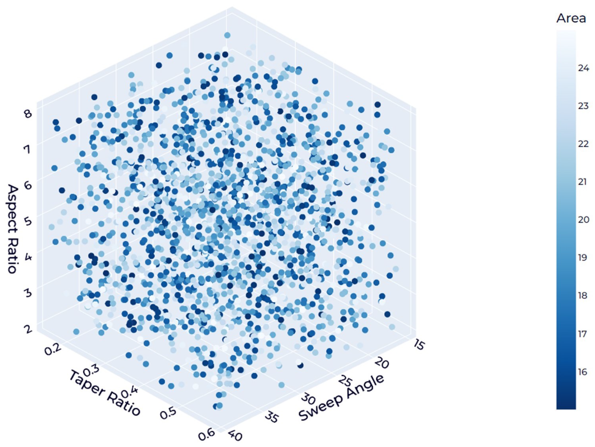
The methodology employed in this work for data generation and sampling integrates various disciplines within a comprehensive aircraft design and analysis framework. This framework enabled the automatic generation of a design space that encompasses hundreds of configurations and their respective performance parameters. In order to ensure a comprehensive and representative sampling of the design space, the Latin hypercube sampling (LHS) method was incorporated into the algorithm. LHS is a statistical method employed to generate a quasi-random sample of plausible collections of parameter values from a multidimensional distribution [78]. This ensures that each parameter is uniformly sampled throughout its range. In Figure 7, it is possible to examine the visualization of the LHS distribution of the four parameters (wing area, aspect ratio, taper ratio, and sweep angle) required to define a wing component. This technique is particularly effective in reducing the number of samples required for accurate statistical representation compared to simple random sampling.

A Python script was developed to implement the algorithm, integrating the NASA open-source parametric model (OpenVSP) API, which allows parametric modeling of the configurations [79,80]. This approach facilitated the parametric setting of vehicle components, enabling detailed and flexible modeling. Furthermore, analysis tools from various disciplines were integrated into the framework, enabling a comprehensive evaluation of different configurations. The developed Python modules integrated the performance parameters obtained from aerodynamic, structural, RCS, and weight models into a single data set. The systematic approach to data generation and sampling was a critical element in developing a reliable artificial neural network model capable of making accurate predictions across a broad spectrum of conditions.

The design space generation algorithm detailed in Algorithm 1 begins by taking the number of configurations ($n_{\mathrm{config}}$) and the parameter limits (${\mathbf{X}}_{\mathrm{limits}}$) as input to produce the final design space dataframe ($\mathit{DF}$). First, the VSP API is initialized, and physical and environmental parameters are defined. The Latin hypercube sampling (LHS) methodology is then employed to generate a quasi-random sampling distribution (S) within the given parameter limits, resulting in a set of configuration vectors (${\mathbf{V}}_{\mathrm{config}}$). For each configuration vector ($\overrightarrow{v_i}$) in the set, the wing, tail, and fuselage geometries are defined using specific geometric parameters. These geometries are then set in the VSP model, which is subsequently updated.

Algorithm 1 Design space generation algorithm.
Input: $n_{\mathrm{config}}$, ${\mathbf{X}}_{\mathrm{limits}}$
Output: $\mathit{DF}$
1:	procedure DesignSpace($n_{\mathrm{config}}$, ${\mathbf{X}}_{\mathrm{limits}}$)
2:	Initialize VSP API
3:	Define physical and environmental parameters
4:	$S\leftarrow \mathrm{initialize}\mathrm{LHS}\mathrm{with}{\mathbf{X}}_{\mathrm{limits}}$
5:	${\mathbf{V}}_{\mathrm{config}}\leftarrow S\left(n_{\mathrm{config}}\right)$
6:	for $i\leftarrow 1\mathrm{to}{n}_{\mathrm{config}}$ do
7:	$\overrightarrow{v_i}\leftarrow \overrightarrow{v_i}\in {\mathbf{V}}_{\mathrm{config}}$
8:	Define wing geometry using $\overrightarrow{v_i}=\{A{R}_{wing},{\lambda }_{wing},{\Lambda }_{wing},{\Gamma }_{wing},A_{wing}\}$
9:	Define tail geometry using $\overrightarrow{v_i}=\{A{R}_{tail},{\lambda }_{tail},{\Lambda }_{tail},{\Gamma }_{tail},A_{tail}\}$
10:	Define fuselage geometry using $\overrightarrow{v_i}=\{l_{fore},l_{mid},l_{aft},d_h\}$
11:	Set geometry using wing, tail, fuselage
12:	Update VSP model
13:	${\mathcal{M}}_{aero}\leftarrow \mathrm{mesh}\overrightarrow{v_i}$
14:	$c_L,c_D,c_M,Q_{aero}\leftarrow$AerodynamicsPerformance$\left({\mathcal{M}}_{aero}\right)$
15:	${\mathcal{M}}_{structural}\leftarrow \mathrm{mesh}\overrightarrow{v_i}$
16:	$W_{structure}\leftarrow$StructuralPerformance$({\mathcal{M}}_{structural},Q_{aero})$
17:	${\mathcal{M}}_{RCS}\leftarrow \mathrm{mesh}\overrightarrow{v_i}$
18:	${\sigma }_{dBsm}\leftarrow$RadarCrossSectionPerformance$\left({\mathcal{M}}_{RCS}\right)$
19:	$W_{empty}\leftarrow$Weights$(\overrightarrow{v_i},W_{structure},c_L,c_D)$
20:	$\overrightarrow{D{F}_i}\leftarrow \overrightarrow{D{F}_i}=\{\overrightarrow{v_i},c_L,c_D,c_M,{\sigma }_{dBsm},W_{structure},W_{empty}\}$
21:	end for
22:	${\mathit{DF}}_{\mathrm{i},\mathrm{j}}\leftarrow \overrightarrow{D{F}_i}\mathrm{concat}\mathrm{for}i=\{1,2,3,\dots ,n_{\mathrm{config}}\}$
23:	return $\mathit{DF}\}$
24:	end procedure
25:	procedure AerodynamicsPerformance(${\mathcal{M}}_{aero}$)
26:	$Re,M,\nu ,\mu ,\alpha \leftarrow \mathrm{Set}\mathrm{flow}\mathrm{conditions}$
27:	Run aerodynamics analysis
28:	return $\{c_L,c_D,c_M\}$
29:	end procedure
30:	procedure StructuralPerformance(${\mathcal{M}}_{structural},Q_{aero}$)
31:	if component = wing or tail then
32:	$E,G,{\sigma }_S\leftarrow \mathrm{Set}\mathrm{analysis}\mathrm{parameters}$
33:	Run structural analysis
34:	Optimize $W_{structure}$
35:	else
36:	Calculate $W_{structure}$
37:	end if
38:	$W_{structure}\leftarrow W_{structure}=W_{wing}+W_{tail}+W_{fus}$
39:	return $W_{structure}$
40:	end procedure
41:	procedure RadarCrossSectionPerformance(${\mathcal{M}}_{RCS}$)
42:	$\theta ,\varphi \leftarrow \mathrm{Set}\mathrm{analysis}\mathrm{parameters}$
43:	Run RCS analysis
44:	return ${\sigma }_{dBsm}$
45:	end procedure
46:	procedure Weights($\overrightarrow{v_i},W_{structure},c_L,c_D$)
47:	Run weights analysis
48:	return $W_{empty}$
49:	end procedure

The algorithm proceeds by performing aerodynamic, structural, radar cross-section (RCS), and weight analyses on each configuration. Aerodynamic performance (coefficients $c_L$, $c_D$, $c_M$, and aerodynamic loads $Q_{aero}$) is evaluated by meshing the geometry (${\mathcal{M}}_{aero}$) and performing the three-dimensional compressible panel method analysis. Structural performance ($W_{structure}$) is determined by meshing the geometry (${\mathcal{M}}_{structural}$), performing the one-dimensional finite element method analysis, and optimizing the structural weight based on aerodynamic loads. The RCS analysis is conducted by meshing the geometry (${\mathcal{M}}_{RCS}$) and running the physical optics (PO) approximation combined with ray tracing. The empty weight ($W_{empty}$) of the configuration is then calculated using the geometric parameters, structural weight, and aerodynamic coefficients.

The results of each analysis ($\overrightarrow{D{F}_i}$), comprising geometric parameters, aerodynamic coefficients, RCS, structural weight, and empty weight, are concatenated to form the design space dataframe ($\mathit{DF}$). The subprocedures “Aerodynamic Performance”, “Structural Performance”, “Radar Cross Section Performance” and “Weights” include specific analysis and provide a modular and systematic approach to evaluate the performance of each configuration within the design space by running relevant tools.

3.3.2. Physics-Informed Feature Engineering

Feature engineering represents a pivotal aspect in enhancing the efficacy of neural network models used for UAV analysis. The process begins with data analysis and the selection of the most relevant features that serve as input to neural networks. Pearson’s correlation analysis is performed to understand the relationships between different characteristics, ensuring that only those with significant impact are retained [81,82]. The correlation coefficient for each future is calculated as follows:

$$r={\displaystyle \frac{\sum (x_i-\overline{x})(y_i-\overline{y})}{\sqrt{\sum {(x_i-\overline{x})}^2\sum {(y_i-\overline{y})}^2}}}$$

(33)

where r is the correlation coefficient, $x_i$ and $y_i$ represent the values of the variables in a sample, and $\overline{x}$ and $\overline{y}$ are the mean values of the variables. Calculated correlations are of great significance in the context of feature selection in data-driven modeling. The identification of variables exhibiting a strong correlation (either positive or negative) facilitates the selection of the most crucial parameters influencing the model’s output, thereby enabling the generation of a more efficient and accurate prediction model.

Figure 8 presents a scatter plot matrix that illustrates the relationships between the target parameters and example future sets of a wing. Each row represents a different target variable: lift coefficient ($C_L$), drag coefficient ($C_D$), radar cross section, and empty weight. Each column represents parameters of geometry and flow conditions. The plots demonstrate that $C_L$ and $C_D$ increase with the angle of attack, in accordance with typical aerodynamic behavior. However, they also exhibit some variation with other parameters, although the trends are less obvious. The RCS exhibits a scattered distribution across all parameters, indicating a complex relationship influenced by multiple factors. The weight appears to vary significantly with geometric parameters such as aspect ratio, reference span, and chord length.

Upon training the model using feature sets related to flow and geometry as previously described, it was observed that the model exhibited limited generalization ability, particularly in aerodynamic performance parameters. This issue was addressed by adding physical information to the algorithm. Incorporating physical information into neural networks can significantly enhance prediction accuracy and reliability, particularly in complex engineering applications such as UAV design. One approach for the artificial neural network to obtain physical information is to include physical constraints directly in the cost function. Formulating the cost function to include terms that penalize deviations from known physical laws directs the neural network to produce physically plausible output. Another method involves augmenting the training data with additional physical information. This can be achieved by creating synthetic data points that satisfy physical equations and adding them to the training data set. For example, combining data points derived from an aerodynamics equation ensures that the neural network is exposed to a wide range of physically correct scenarios during training. This approach enables the neural network to learn the underlying physical relationships more effectively.

In this work, an empirical lift-curve slope was calculated using other geometric features and provided to the algorithm with the objective of enhancing the generalizability of the lift coefficient. In order to achieve this objective, the compressible form of the Helmbold–Diederich equation, which was developed for a thin-section swept planform, was employed [83,84]. The general form of this equation is as follows:

$$a={\displaystyle \frac{2\pi AR}{2+\sqrt{{(\beta ·AR)}^2+{\left(AR·tan{\Lambda }_{1/2}\right)}^2+4}}}$$

(34)

where $\beta =\sqrt{1-M^2}$ is the Prandtl–Glauert compressibility factor. In the application of this equation, the quarter-chord sweep angle (${\Lambda }_{1/4}$) is commonly used due to its consistency and historical validation in calculating aerodynamic coefficients such as lift-curve slopes [85]. However, the half-chord sweep angle (${\Lambda }_{1/2}$) can provide a better correlation with the lifting surface theory, particularly in scenarios with significant wing taper, as it helps reduce scatter and improve accuracy by effectively accounting for the impact of the taper on aerodynamic properties [86]. ESDU TM 169 indicates that the use of the half-chord sweep angle (${\Lambda }_{1/2}$) improves the correlation of lift-curve slope data with theoretical predictions, rendering it advantageous for complex wing geometries [87]. It is also important to note that this approach is valid for a sweep angle of up to 60 degrees.

3.3.3. Multilayer Perceptron-Based Network Architecture

Neural network algorithms were employed to train the black-box model using a multilayer perceptron (MLP) structure to regress the performance data Y based on the input features X. A fully connected network with L hidden layers is described by modeling equations that relate the input features x to their target predictions y. The neural network consists of M input features and N layers, with each layer composed of neurons performing a series of mathematical operations followed by nonlinear activation functions.

The model parameters $\xi$ are defined as $\xi =\{W,b\}$, where $W={\left\{w_i\right\}}_{i=1}^N$ and $b={\left\{b_i\right\}}_{i=1}^N$. The output of the l-th layer is given by

$$f(x,{\xi }_l)=f_{w_l,b_l}\left(x\right)=z_l\left(\sum _{j=1}^{N_l}{w}_{lj}{x}_j+b_l\right)=Z_l\left(w_l^T{x}_l+b_l\right)(l=1,\dots ,N)$$

(35)

In this equation, $N_l$ is the number of neurons in the l-th layer, $Z_l$ is the nonlinear activation function of the l-th layer, and $x_l$ is the input to the l-th layer, which is also the output of the $(l-1)$-th layer. The parameters $w_l$ and $b_l$ are the learnable weights and biases of the l-th layer, respectively.

The final output of the neural network, $\widehat{y}\left(x\right)$, is the result of a complex and composite mapping defined as

$$\widehat{y}\left(x\right):=\left(f_{w_N,b_N}\circ f_{w_{N-1},b_{N-1}}\circ \cdots \circ f_{w_1,b_1}\right)\left(x\right)$$

(36)

In the implemented neural network architecture, the input layer accepts features with shape $(n\_features)$. The first hidden layer, $L1$, consists of 512 neurons with a sigmoid activation function and weights initialized using the “the normal” method:

$$L_1=\sigma \left(W_{1}x+b_1\right)$$

(37)

where $\sigma$ denotes the sigmoid activation function, $W_1$ is the weight matrix, and $b_1$ is the bias vector for the first layer. The sigmoid activation function is defined as

$$\sigma \left(z\right)={\displaystyle \frac{1}{1+e^{-z}}}$$

(38)

The subsequent layers follow a similar structure:

$$\begin{array}{cc}\hfill L_2=& \sigma \left(W_2{L}_1+b_2\right)\hfill \\ \hfill & ⋮\hfill \\ \hfill L_{n-1}=& \sigma \left(W_{n-1}{L}_{n-2}+b_{n-1}\right)\hfill \end{array}$$

(39)

The output layer consists of a single neuron with a linear activation function, resulting in the final prediction:

$$\widehat{y}=W_n{L}_{n-1}+b_n$$

(40)

The model is compiled using the Yogi optimizer with parameters ${\beta }_1=0.9$ and ${\beta }_2=0.999$, and it optimizes the mean absolute error (MAE) loss function [88]. The Yogi optimizer updates the model parameters as follows:

$$m_t={\beta }_1{m}_{t-1}+(1-{\beta }_1)g_t$$

(41)

$$v_t=v_{t-1}-(1-{\beta }_2)\mathrm{sign}(v_{t-1}-g_t^2)g_t^2$$

(42)

$${\widehat{m}}_t={\displaystyle \frac{m_t}{1-{\beta }_1^t}},{\widehat{v}}_t={\displaystyle \frac{v_t}{1-{\beta }_2^t}}$$

(43)

$${\theta }_{t+1}={\theta }_t-{\displaystyle \frac{\eta }{\sqrt{{\widehat{v}}_t}+ϵ}}{\widehat{m}}_t$$

(44)

where $m_t$ and $v_t$ are the first- and second-moment estimates, respectively, ${\beta }_1$ and ${\beta }_2$ are the exponential decay rates for these estimates, $g_t$ is the gradient at the time step t, $\eta$ is the learning rate, and $ϵ$ is a small constant to prevent division by zero. The mean absolute error (MAE) is defined as

$$\mathrm{MAE}={\displaystyle \frac{1}{n}}\sum _{i=1}^n\left|y_i-{\widehat{y}}_i\right|$$

(45)

The Yogi optimizer ensures the efficient and stable convergence of the neural network model parameters. This approach ensures that the architectural network is able to identify and capture complex relationships within the data, allowing accurate predictions of the performance metric Y. The training results of the neural networks developed are presented in the following sections, along with an example of a UAV performance analysis application.

3.4. Multiobjective Genetic Algorithm

In this work, a multiobjective genetic algorithm (MOGA) was employed to optimize the design parameters. Genetic algorithms are robust optimization techniques inspired by the principles of natural selection and genetics. They are particularly effective for solving complex, multiobjective optimization problems where multiple conflicting objectives need to be simultaneously satisfied.

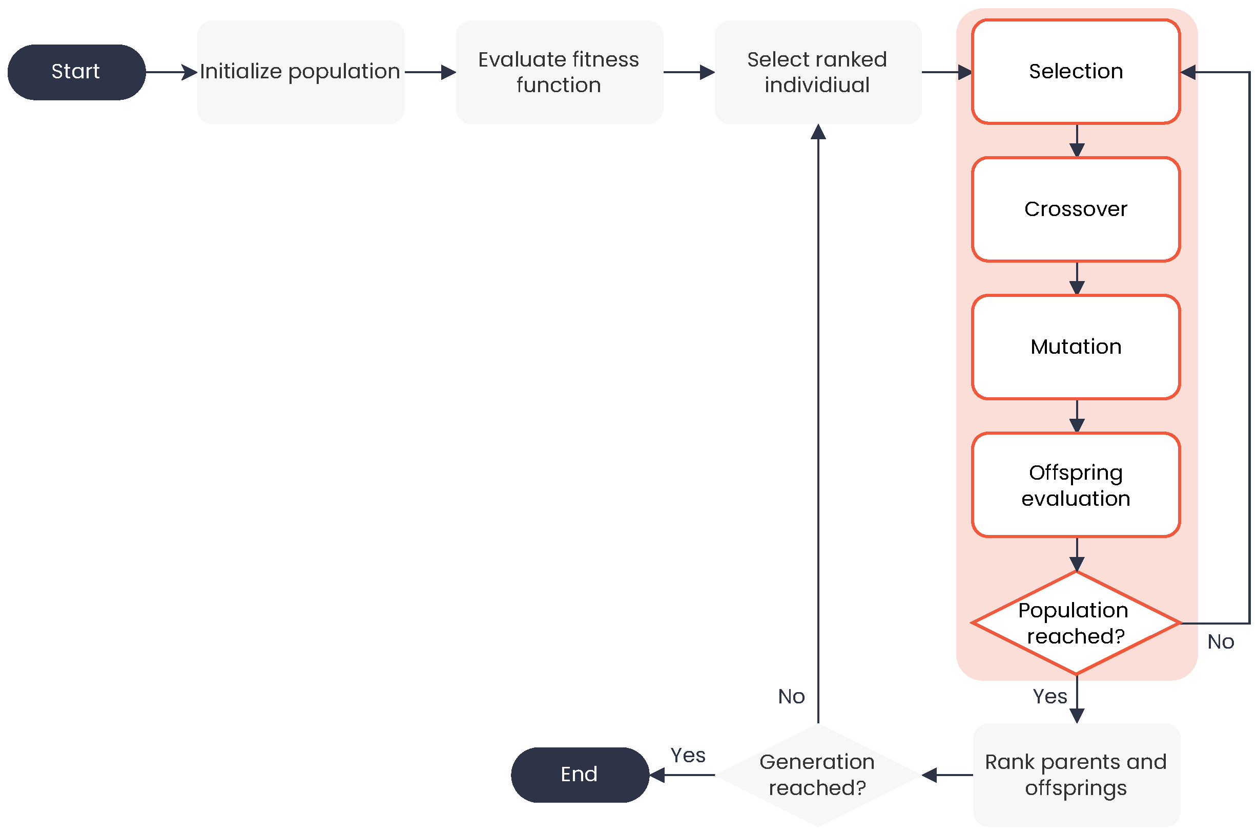
The optimization algorithm utilized in this research comprises a series of essential steps, as illustrated in Figure 9. First, a population of potential solutions is randomly generated within the defined parameter space. Each solution, also known as an individual, is represented by a chromosome that encodes the design variables. Subsequently, each individual within the population is evaluated based on a number of objective functions. These functions assess the performance of the design with regard to criteria such as aerodynamic efficiency, radar cross section (RCS), and structural weight. Individuals are selected for reproduction based on their fitness, with a preference given to those with higher fitness scores. This ensures that high-quality solutions are propagated through successive generations. Pairs of selected individuals undergo a crossover, exchanging portions of their chromosomes to produce offspring. This process introduces novel genetic combinations and expands the search space for potential solutions. Additionally, the offspring are subjected to random mutations, whereby minor alterations are made to their chromosomes. Mutation serves to maintain genetic diversity within the population, thereby preventing premature convergence to local optima. The population is sorted into distinct fronts based on the principle of Pareto dominance. The crowding distance is calculated in order to maintain diversity among solutions on the same front. Individuals with superior ranks and elevated crowding distances are selected for the subsequent generation. The current population is replaced by the new generation of individuals, and the process iterates until a termination criterion is met, such as a maximum number of generations or convergence of the Pareto front.

The specific implementation of the MOGA in this work used the Nondominated Sorting Genetic Algorithm II (NSGA-II), which is well-known for its efficiency in handling multiobjective optimization problems [89]. The algorithm was implemented using a versatile optimization library in Python [90]. The application of NSGA-II resulted in a diverse set of optimized design configurations. The Pareto front obtained demonstrates the trade-offs between conflicting objectives, providing valuable insights for decision makers. Key performance indicators such as aerodynamic lift-to-drag ratio, structural weight efficiency, and radar cross section were significantly improved through the optimization process.

4. Application of the Model

An example design problem was discussed to implement the model. The application focused on the previously mentioned high-performance UAVs. A list of requirements was determined for a generic design capable of long-range flight, operating at high subsonic speeds, and mounting various internal payload systems.

The requirements for the proposed aerial system are listed as follows:

• Maximum take-off weight: 3000 kg
• Payload weight: 500 kg
• Cruise speed: 0.7 Mach
• Endurance: 5 h
• Range: 3000 NM
• Maximum altitude: 45,000 ft

The requirements were used as input to the initial design algorithm to make the preliminary estimates necessary for the initial sizing of the aircraft. In order to create the design space, the maximum and minimum ranges of the design variables are determined and provided as input to the neural network algorithm.

Table 3. Design variable ranges for conceptual design space exploration.

	Parameter	Symbol	Units	Minimum	Maximum
Wing	Wing area	A	${\mathrm{m}}^2$	15	25
	Aspect ratio	$AR$	−	2	8
	Taper ratio	$\lambda$	−	0.2	0.6
	Sweep	$\Lambda$	°	15	40
	Length	l	m	5	15
	Hydraulic diameter	$d_h$	m	1	2
Fuselage	Fineness ratio	f	−	2.5	15
Engine	Thrust	T	kN	5	20
	Angle of attack	$\alpha$	°	0	4
	Mach number	M	−	0.6	0.8
Flow condition	Reynolds number	$Re$	−	$6·{10}^6$	$18·{10}^6$

shows the ranges of design variables identified for concept design space exploration. These parameters are grouped into four main categories: wing, fuselage, engine thrust, and flow conditions. The design space is constrained so that the solution point of the wing area obtained from the initial design algorithm covers the perimeter of the prediction. It is possible to model any one-piece wing with aspect ratio, taper, and sweep. The hydraulic diameter and the fineness ratio were considered for the fuselage modeling. The maximum thrust value for the engine was obtained from the initial design algorithm, similar to the wing area. Flow conditions were determined to cover the target flight regime at cruising altitude. As a result, performance models were obtained following the data generation and artificial neural network training described in the previous sections.

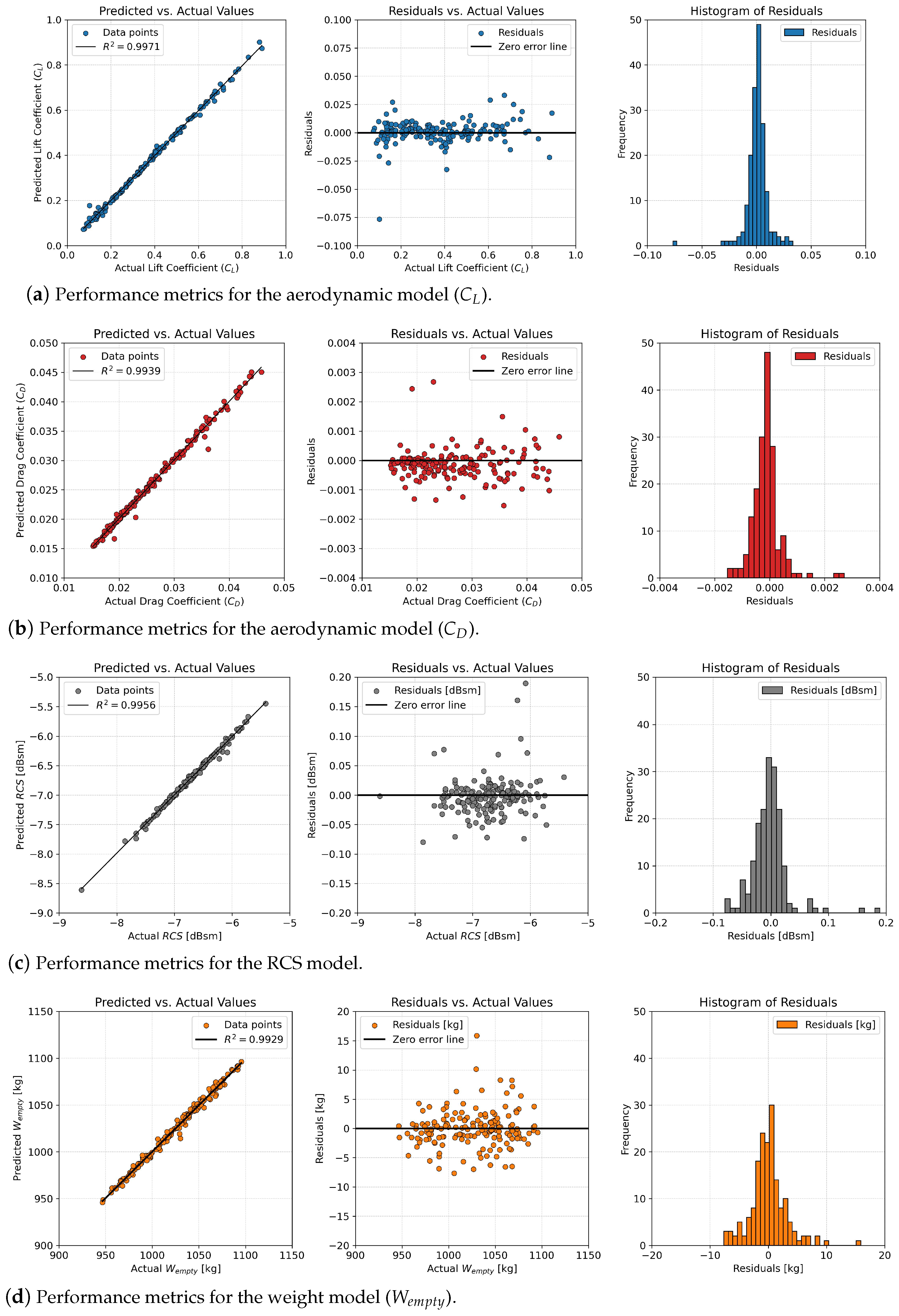
The results of the performance evaluation of neural network models in predicting aerodynamic coefficients, radar cross-section, and weight characteristics are presented in Figure 10, which contains several key subfigures. Figure 10a illustrates the predicted versus actual lift coefficient ($C_L$) values, showcasing an exceptional fit with an $R^2$ value of 0.9971. The residuals plot reveals a minimal deviation from the actual values, with residuals clustering closely around the zero-error line and a maximum residual of approximately $\pm 0.075$. The histogram of residuals displays a symmetric distribution centered around zero, indicating that the majority of predictions are highly accurate and demonstrating the model’s robustness in predicting lift coefficients. Figure 10b presents the predicted versus actual drag coefficient ($C_D$) values, indicating a strong correlation with an $R^2$ value of 0.9939. The residuals plot exhibits a tight distribution around the zero-error line, with a maximum residual of approximately $\pm 0.003$. The residual histogram further confirms the accuracy of the model, with most residuals clustering near zero. Figure 10c evaluates the predicted versus actual radar cross-section (RCS) values. An $R^2$ value of 0.9956 suggests robust model performance. The residual plot and the corresponding histogram show that most predictions are accurate, with residuals closely aligned with the zero-error line and a maximum residual of approximately $\pm 0.15$. The narrow spread of residuals in the histogram signifies the model’s consistent reliability in predicting RCS values. Lastly, Figure 10d compares the predicted versus actual empty weight values, giving an $R^2$ value of 0.9929. The residual plot demonstrates that the predictions are generally accurate, with minor deviations from the actual values and a maximum residual of around $\pm 20$ kg. The residual histogram supports this observation, showing a concentration of residuals around zero.

The collective results demonstrate the effectiveness of neural network models in accurately predicting critical aerodynamics, radar cross-section, and weight parameters. The current margins of error are below acceptable levels in the early design stages. The high values of the correlation coefficient, $R^2$, and the narrow distributions of residuals in all models demonstrate the robust precision of the neural network approach utilized in this investigation. Once the data-driven models have been obtained, the subsequent step is to define the objective functions and constraints that are necessary for the execution of the multiobjective genetic algorithm. The optimization process focuses on improving the design of a high-performance UAV by simultaneously addressing multiple conflicting objectives. The optimization problem identified for this specific application can be summarized as follows:

$$\begin{array}{cc}\hfill \underset{\begin{array}{c}x\in \overrightarrow{V}=\{\lambda ,AR,\Lambda ,\dots \}\hfill \\ y\in \overrightarrow{U}=\{\alpha ,M,Re,\dots \}\hfill \end{array}}{\mathrm{minimize}}F& =\{f_1(x,y),f_2\left(x\right),f_3(x,y)\}\hfill \\ \hfill \mathrm{where}{f}_1(x,y)& =-{\displaystyle \frac{C_L}{C_D}}\hfill \\ \hfill f_2\left(x\right)& =\mathrm{RCS}\hfill \\ \hfill f_3(x,y)& =W_{\mathrm{empty}}\hfill \\ \hfill \mathrm{subject}\mathrm{to}0.2& \le \lambda \le 0.6\hfill \\ \hfill 4& \le AR\le 8\hfill \\ \hfill {15}^{\circ }& \le \Gamma \le {40}^{\circ }\hfill \\ \hfill 0^{\circ }& \le \alpha \le 2^{\circ }\hfill \end{array}$$

(46)

where the objective functions include maximizing the lift-to-drag ratio, minimizing the radar cross section, and minimizing the empty weight of the UAV. These objectives are essential to improve aerodynamic efficiency, stealth capabilities, and overall performance. While a wing structure with a high span ratio is required to increase aerodynamic efficiency, a wing with a lower span ratio and angle of attack is required to minimize structural weight. While stealth performance increases with the sweep angle, it also changes with the overall shape of the vehicle. It is possible to search for wing configurations with different planforms such as tapered, sweptback, and delta in the current design space. Optimization variables such as the taper ratio, the aspect ratio, the sweep angle, and the angle of attack are constrained within certain ranges to ensure realistic and feasible design solutions.

5. Results

The problem is solved using a multiobjective genetic algorithm, which efficiently explores the design space and finds a diverse set of optimal solutions along the Pareto front. This approach provides valuable insight into the trade-offs between different design objectives, allowing the selection of the most balanced and effective UAV configurations. The optimization process is performed using the Nondominated Sorting Genetic Algorithm II (NSGA-II) with a population size of 50 and an iteration criterion of 200 generations.

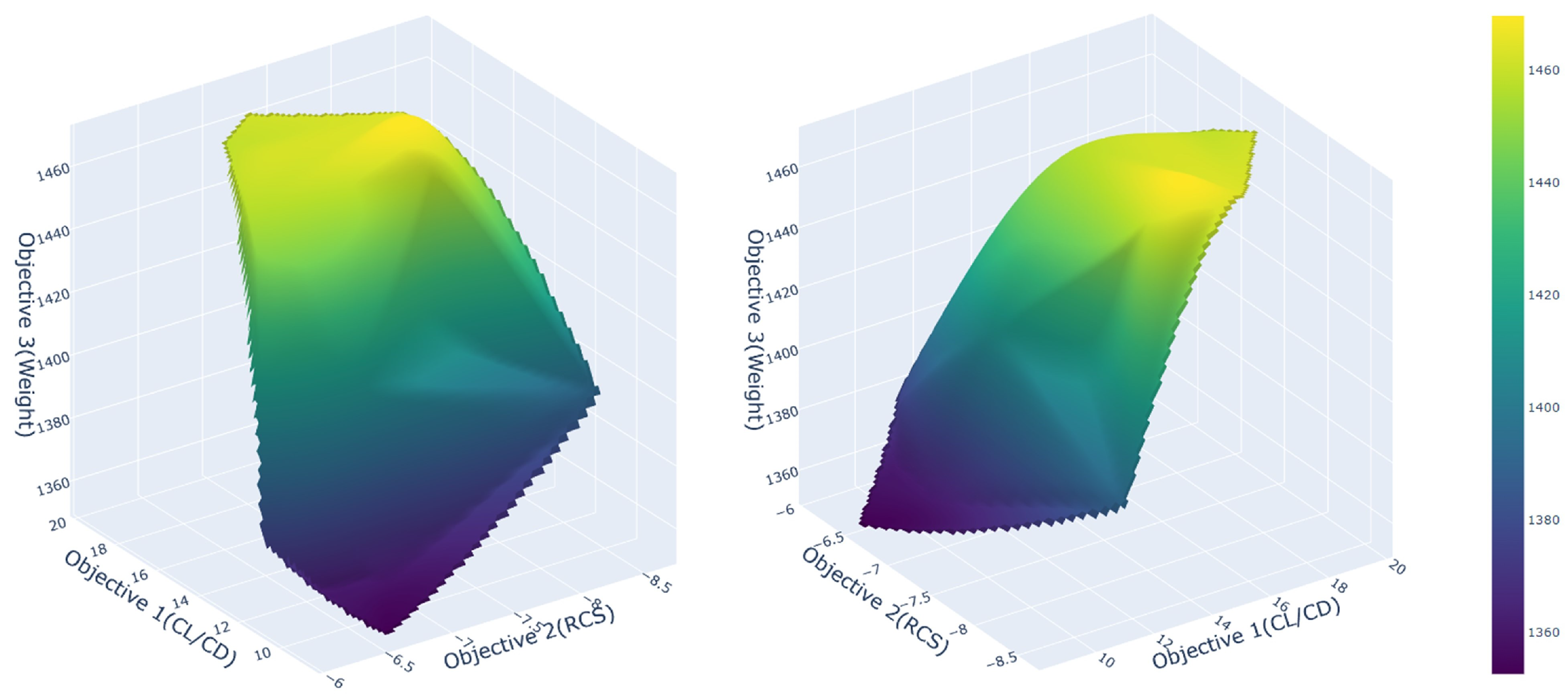
As a result of the optimization, the Pareto front surface shown in Figure 11 was obtained. The given three-dimensional surface plots illustrate the trade-offs between three key objectives: maximizing the lift-to-drag ratio (CL/CD), minimizing the radar cross section (RCS), and minimizing the empty weight. The color gradient from blue to yellow represents different levels of the third objective (empty weight). The smooth and continuous surface of the Pareto front indicates a well-defined and consistent set of optimal solutions generated by the NSGA-II algorithm.

Three configurations maximizing each objective from the Pareto front solution were considered and compared based on the performance metrics determined. These performance metrics are defined as endurance, range, speed, maneuverability, stealth, and payload. Representative models of the configurations and the radar plot are shown in Figure 12. In the figure, the configuration numbers are presented in a sorted order according to the objective. The optimal configuration for aerodynamic efficiency is Configuration 1, while Configuration 2 is the most effective in minimizing the radar cross section (RCS) and Configuration 3 is the lowest in empty weight. Configuration 1 (shown in blue) exhibits a remarkable degree of success in endurance and range measurements, performing approximately 43% better in aerodynamic efficiency. It can be observed that this concept is more suitable for mission profiles such as ISR. Additionally, stealth and payload are sufficient to carry surveillance equipment while avoiding detection. Configuration 2 (in yellow) demonstrates the overall performance in other metrics while exhibiting superior stealth performance with $-8.69dBsm\approx 0.1357m^2$ RCS. The high scores in stealth, speed, and maneuverability make Configuration 2 an optimal choice for SEAD and tactical strike missions where rapid maneuvers and low detectability are paramount. Configuration 3 (red) scores high both in speed and maneuverability with an empty weight of approximately 1350 kg, indicating a design optimized for agile and fast operations. However, this design compromises on endurance and range. The configuration exhibits the highest performance in speed and maneuverability, accompanied by a high payload, making it suitable for combat air patrol (CAP) missions where agility and rapid response are paramount.

The design process, which leveraged advanced AI models, was remarkably efficient, requiring a total of just 4–5 s to complete. This rapid optimization was accomplished through the utilization of a personal laptop, equipped with an Intel Core i7-11800H processor and 32 GB of RAM. The deployment of AI-driven models markedly accelerated the assessment of design solutions, facilitating quick navigation through the intricate design space. In contrast, had traditional methodologies been employed, the optimization process would have taken 4–5 h to achieve comparable results with the same computational environment.

6. Conclusions

In this work, we demonstrated the application of advanced deep neural networks to the multidisciplinary conceptual design of UAVs. The goal was to enhance the design process by leveraging AI to optimize various performance metrics, including aerodynamic efficiency, stealth capabilities, and structural weight. By employing a multiobjective genetic algorithm integrated with AI-driven models, we efficiently explored the design space and identified a set of optimal UAV configurations. The proposed design process was completed in just a couple of seconds. This represents an improvement of more than three orders of magnitude compared to traditional methods, which would have required computational times of the order of hours to achieve comparable results. A state-of-the-art physics-informed feature engineering approach was employed to develop precise surrogate models, which accurately predict critical UAV performance metrics such as aerodynamic efficiency, stealth capabilities, and structural integrity. The results show significant advantages of this AI-based approach. The AI models enabled a rapid and precise evaluation of design solutions, facilitating a comprehensive understanding of the trade-offs between different design objectives. The Pareto front generated from the optimization process provided valuable insights into the optimal balance between lift-to-drag ratio, radar cross section, and structural weight. Furthermore, the research tailors UAV designs to specific mission profiles by addressing unique operational requirements, ensuring each configuration excels in its intended application, such as ISR, SEAD, or CAP missions. In the example application, three UAV configurations were identified and analyzed based on their performance in six key parameters: endurance, range, speed, maneuverability, stealth, and payload. Configuration 1, with its high endurance and range, is well suited for intelligence, surveillance, and reconnaissance (ISR) missions. Configuration 2, which excels in stealth, speed, and maneuverability, is ideal for Suppression of Enemy Air Defenses (SEAD) and tactical strike missions. Configuration 3, optimized for speed and maneuverability, is best suited for combat air patrol (CAP) missions.

The integration of AI in the UAV design process offers substantial benefits, including significant reductions in computational time and enhanced flexibility to explore complex design spaces. This approach not only facilitates rapid prototyping and iterative design but also paves the way for more efficient and effective engineering solutions in the aerospace industry. The potential for AI-driven optimization to revolutionize UAV design and address other multidisciplinary engineering challenges is considerable and continues to evolve.

References

1. Cummings, R.M.; Mason, W.H.; Morton, S.A.; McDaniel, D.R. Applied Computational Aerodynamics: A Modern Engineering Approach; Cambridge Aerospace Series; Cambridge University Press: Cambridge, UK, 2015. [Google Scholar] [CrossRef]
2. Jungo, A.; Zhang, M.; Vos, J.B.; Rizzi, A. Benchmarking New CEASIOM with CPACS adoption for aerodynamic analysis and flight simulation. Aircr. Eng. Aerosp. Technol. 2018, 90, 613–626. [Google Scholar] [CrossRef]
3. Roskam, J. Airplane Design; DARcorporation: St. Lawrence, KS, USA, 1985. [Google Scholar]
4. Raymer, D. Aircraft Design: A Conceptual Approach; American Institute of Aeronautics and Astronautics Inc.: Las Vegas, NV, USA, 2012. [Google Scholar]
5. Sadraey, M.H. Aircraft Design: A Systems Engineering Approach; Aerospace Series; John Wiley and Sons: Chichester, UK, 2013. [Google Scholar] [CrossRef]
6. de Weck, O.; Willcox, K. Multidisciplinary System Design Optimization. 2003. Available online: https://ocw.mit.edu/courses/ids-338j-multidisciplinary-system-design-optimization-spring-2010/ (accessed on 10 June 2022).
7. Roth, G.L.; Altman, A. Re-imagining Engineering Conceptual Design for Aerospace. In Proceedings of the AIAA AVIATION 2022 Forum, Chicago, IL, USA, 27 June–1 July 2022; p. 3880. [Google Scholar]
8. Liao, P.; Song, W.; Du, P.; Feng, F.; Zhang, Y. Aerodynamic Intelligent Topology Design (AITD)-A Future Technology for Exploring the New Concept Configuration of Aircraft. Aerospace 2023, 10, 46. [Google Scholar] [CrossRef]
9. Asimov, I. I, Robot; Doubleday: New York, NY, USA, 1950. [Google Scholar]
10. Stanisław, L. The Invincible; Seabury Press: New York, NY, USA, 1973. [Google Scholar]
11. Humphreys, C.; Cobb, R.; Jacques, D.; Reeger, J. Optimal Mission Path for the Uninhabited Loyal Wingman. In Proceedings of the 16th AIAA/ISSMO Multidisciplinary Analysis and Optimization Conference, Dallas, TX, USA, 22–26 June 2015; p. 2792. [Google Scholar]
12. Stensrud, R.; Mikkelsen, B.; Betten, S.; Valaker, S. A proposal for a simple evaluation method in support of the initial concept phase assessing a future unmanned Loyal Wingman for Royal Norwegian Air Force (RNoAF). In Proceedings of the 38th International Symposium on Military Operational Research (38 ISMOR), Online, 20–21 July 2021. [Google Scholar]
13. Harper, J. The Rise of Skyborg: Air Force Betting on New Robotic Wingman. Natl. Def. 2020. Available online: https://www.nationaldefensemagazine.org/articles/2020/9/25/air-force-betting-on-new-robotic-wingman#:~:text=The%20Rise%20of%20Skyborg%3A%20Air%20Force%20Betting%20on%20New%20Robotic%20Wingman&text=The%20next%20year%20will%20be,will%20soon%20undergo%20operational%20experimentation (accessed on 11 August 2024).
14. Gunzinger, M.; Autenried, L. Understanding the Promise of Skyborg and Low-Cost Attritable Unmanned Aerial Vehicles. Mitchell Inst. Policy Pap. 2020, 24. Available online: https://mitchellaerospacepower.org/understanding-the-promise-of-skyborg-and-low-cost-attritable-unmanned-aerial-vehicles/ (accessed on 11 August 2024).
15. Reim, G. Analysis: US Air Force eyes adoption of ‘Loyal Wingman’ UAVs. Flight Glob. 2018. Available online: https://www.flightglobal.com/analysis/analysis-us-air-force-eyes-adoption-of-loyal-wingman-uavs/129330.article (accessed on 11 August 2024).
16. Smith, A.; Rogers, M. F-35 Sustainment: DOD Needs to Cut Billions in Estimated Costs to Achieve Affordability; U.S. Government Accountability Office: Washington, DC, USA, 2021.
17. Colombi, J.; Bentz, B.; Recker, R.; Lucas, B.; Freels, J. Attritable design trades: Reliability and cost implications for unmanned aircraft. In Proceedings of the 2017 Annual IEEE International Systems Conference (SysCon), Montreal, QC, Canada, 24–27 April 2017; IEEE: New York, NY, USA, 2017; pp. 1–8. [Google Scholar]
18. Pittaway, N. Boeing details MQ-28A payload ground test phase. Aust. Def. Mag. 2022. Available online: https://www.australiandefence.com.au/defence/air/boeing-details-mq-28a-payload-ground-test-phase#:~:text=A%20variety%20of%20payloads%20will,of%20the%20aircraft%27s%20removable%20nose (accessed on 11 August 2024).
19. Newdick, T. The United Kingdom Has Chosen Who Will Build Its First Prototype Loyal Wingman Combat Drone. Drive Warzone 2021. Available online: https://www.thedrive.com/the-war-zone/42134/the-united-kingdom-has-chosen-who-will-build-its-first-prototype-loyal-wingman-combat-drone (accessed on 11 August 2024).
20. Aviation Week. EADS Barracuda. Available online: https://aviationweek.com/defense-space/eads-cassidian-eyes-further-barracuda-uav-flights (accessed on 26 May 2024).
21. 96th Test Wing, 40th Flight Test Squadron. Kratos XQ-58. Photo by Master Sgt. Tristan McIntire. Available online: https://www.flightglobal.com/military-uavs/usmc-completes-first-test-flight-with-autonomous-xq-58/155257.article (accessed on 26 May 2024).
22. Australian Defense Department. MQ-28 Loyal Wingman. Available online: https://aviationweek.com/shownews/farnborough-airshow/boeings-phantom-works-wants-untethered-loyal-wingman (accessed on 26 May 2024).
23. Anadolu Images. Baykar Kizilelma. Available online: https://www.aa.com.tr/tr/bilim-teknoloji/bayraktar-kizilelma-ilk-ucusunu-gerceklestirdi/2763872 (accessed on 26 May 2024).
24. General Atomics. XQ-67A Off Board Sensing Station Maiden Flight over Palmdale, California. Available online: https://www.dvidshub.net/image/8275788/afrls-xq-67a-makes-1st-successful-flight (accessed on 26 May 2024).
25. Qinetiq. Qinetiq Derives Collaborative UAS from Banshee Target. Credit: Qinetiq. Available online: https://aviationweek.com/defense-space/aircraft-propulsion/qinetiq-derives-collaborative-uas-banshee-target (accessed on 26 May 2024).
26. BAE Systems. UAS Concepts. 2023. Available online: https://www.baesystems.com/en/product/uas-concepts (accessed on 26 May 2024).
27. Air & Space Forces Magazine. Anduril and General Atomics to Develop New Collaborative Combat Aircraft for Air Force. The Anduril “Fury” Autonomous Aircraft on April 24. Courtesy Photo. Available online: https://www.airandspaceforces.com/cca-contract-winners-to-be-announced-imminently/ (accessed on 11 August 2024).
28. Sobieszczanski-Sobieski, J. Multidisciplinary design optimization: An emerging new engineering discipline. In Advances in Structural Optimization; Springer: Berlin/Heidelberg, Germany, 1995; pp. 483–496. [Google Scholar]
29. Nguyen, N.V.; Choi, S.M.; Kim, W.S.; Lee, J.W.; Kim, S.; Neufeld, D.; Byun, Y.H. Multidisciplinary unmanned combat air vehicle system design using multi-fidelity model. Aerosp. Sci. Technol. 2013, 26, 200–210. [Google Scholar] [CrossRef]
30. Karali, H.; Inalhan, G.; Umut Demirezen, M.; Adil Yukselen, M. A new nonlinear lifting line method for aerodynamic analysis and deep learning modeling of small unmanned aerial vehicles. Int. J. Micro Air Veh. 2021, 13, 17568293211016817. [Google Scholar] [CrossRef]
31. Ng, L.W.; Willcox, K.E. Multifidelity approaches for optimization under uncertainty. Int. J. Numer. Methods Eng. 2014, 100, 746–772. [Google Scholar] [CrossRef]
32. Brunton, S.L.; Nathan Kutz, J.; Manohar, K.; Aravkin, A.Y.; Morgansen, K.; Klemisch, J.; Goebel, N.; Buttrick, J.; Poskin, J.; Blom-Schieber, A.W.; et al. Data-driven aerospace engineering: Reframing the industry with machine learning. AIAA J. 2021, 59, 2820–2847. [Google Scholar] [CrossRef]
33. AIAA Digital Engineering Integration Committee. Digital Twin: Definition & Value—An AIAA and AIA Position Paper; AIAA: Reston, VA, USA, 2020. [Google Scholar]
34. Dantas de Jesus Ferreira, J.A.; Secco, N.R. Decision tree classifiers for unmanned aircraft configuration selection. Aircr. Eng. Aerosp. Technol. 2021, 93, 1122–1132. [Google Scholar] [CrossRef]
35. Sharma, R.S.; Hosder, S. Investigation of aircraft design space exploration with machine learning. In Proceedings of the AIAA Scitech 2021 Forum, Virtual, 11–15 & 19–21 January 2021; p. 0114. [Google Scholar]
36. Oroumieh, M.A.A.; Malaek, S.M.B.; Ashrafizaadeh, M.; Taheri, S.M. Aircraft design cycle time reduction using artificial intelligence. Aerosp. Sci. Technol. 2013, 26, 244–258. [Google Scholar] [CrossRef]
37. Boutemedjet, A.; Samardžić, M.; Rebhi, L.; Rajić, Z.; Mouada, T. UAV aerodynamic design involving genetic algorithm and artificial neural network for wing preliminary computation. Aerosp. Sci. Technol. 2019, 84, 464–483. [Google Scholar] [CrossRef]
38. Setayandeh, M.R. Surrogate model–based robust multidisciplinary design optimization of an unmanned aerial vehicle. J. Aerosp. Eng. 2021, 34, 04021029. [Google Scholar] [CrossRef]
39. Bekemeyer, P.; Bertram, A.; Hines Chaves, D.A.; Dias Ribeiro, M.; Garbo, A.; Kiener, A.; Sabater, C.; Stradtner, M.; Wassing, S.; Widhalm, M.; et al. Data-driven aerodynamic modeling using the DLR SMARTy toolbox. In Proceedings of the AIAA Aviation 2022 Forum, Chicago, IL, USA, 27 June–1 July 2022; p. 3899. [Google Scholar]
40. Sharma, R.S.; Hosder, S. Mission-Driven Inverse Design of Blended Wing Body Aircraft with Machine Learning. Aerospace 2024, 11, 137. [Google Scholar] [CrossRef]
41. Wu, P.; Yuan, W.; Ji, L.; Zhou, L.; Zhou, Z.; Feng, W.; Guo, Y. Missile aerodynamic shape optimization design using deep neural networks. Aerosp. Sci. Technol. 2022, 126, 107640. [Google Scholar] [CrossRef]
42. Yan, X.; Zhu, J.; Kuang, M.; Wang, X. Aerodynamic shape optimization using a novel optimizer based on machine learning techniques. Aerosp. Sci. Technol. 2019, 86, 826–835. [Google Scholar] [CrossRef]
43. Li, J.; Du, X.; Martins, J.R. Machine learning in aerodynamic shape optimization. Prog. Aerosp. Sci. 2022, 134, 100849. [Google Scholar] [CrossRef]
44. Bouhlel, M.A.; He, S.; Martins, J.R. Scalable gradient–enhanced artificial neural networks for airfoil shape design in the subsonic and transonic regimes. Struct. Multidiscip. Optim. 2020, 61, 1363–1376. [Google Scholar] [CrossRef]
45. Du, X.; He, P.; Martins, J.R. A B-spline-based generative adversarial network model for fast interactive airfoil aerodynamic optimization. In Proceedings of the AIAA Scitech 2020 Forum, Orlando, FL, USA, 6–10 January 2020; p. 2128. [Google Scholar]
46. Li, J.; Zhang, M. Data-based approach for wing shape design optimization. Aerosp. Sci. Technol. 2021, 112, 106639. [Google Scholar] [CrossRef]
47. Barnhart, S.A.; Narayanan, B.; Gunasekaran, S. Blown wing aerodynamic coefficient predictions using traditional machine learning and data science approaches. In Proceedings of the AIAA Scitech 2021 Forum, Virtual, 11–15 & 19–21 January 2021; p. 0616. [Google Scholar]
48. Yuan, Y.; Dongli, M.; Muqing, Y.; Zhang, L.; Yang, G. Adaptive-surrogate-based robust optimization of transonic natural laminar flow nacelle. Chin. J. Aeronaut. 2021, 34, 36–52. [Google Scholar]
49. Yu, B.; Xie, L.; Wang, F. An improved deep convolutional neural network to predict airfoil lift coefficient. In Proceedings of the International Conference on Aerospace System Science and Engineering; Springer: Berlin/Heidelberg, Germany, 2019; pp. 275–286. [Google Scholar]
50. Zhang, Y.; Sung, W.J.; Mavris, D.N. Application of convolutional neural network to predict airfoil lift coefficient. In Proceedings of the 2018 AIAA/ASCE/AHS/ASC Structures, Structural Dynamics, and Materials Conference, Kissimmee, FL, USA, 8–12 January 2018; p. 1903. [Google Scholar]
51. Wu, M.Y.; Yuan, X.Y.; Chen, Z.H.; Wu, W.T.; Hua, Y.; Aubry, N. Airfoil shape optimization using genetic algorithm coupled deep neural networks. Phys. Fluids 2023, 35, 085140. [Google Scholar] [CrossRef]
52. Keane, A.J.; Voutchkov, I.I. Surrogate approaches for aerodynamic section performance modeling. AIAA J. 2020, 58, 16–24. [Google Scholar] [CrossRef]
53. Karali, H.; Inalhan, G.; Tsourdos, A. AI-Based Multifidelity Surrogate Models to Develop Next Generation Modular UCAVs. In Proceedings of the AIAA Scitech 2023 Forum, National Harbor, MD, USA, 23–27 January 2023. [Google Scholar] [CrossRef]
54. Karali, H.; Inalhan, G.; Tsourdos, A. AI-driven Unmanned Aerial System Conceptual Design with Configuration Selection. In Proceedings of the 2023 IEEE Conference on Artificial Intelligence (CAI), Santa Clara, CA, USA, 5–6 June 2023; IEEE: New York, NY, USA, 2023; pp. 83–84. [Google Scholar] [CrossRef]
55. Karali, H.; Inalhan, G.; Tsourdos, A. AI-Driven Multidisciplinary Conceptual Design of Unmanned Aerial Vehicles. In Proceedings of the AIAA SCITECH 2024 Forum, Orlando, FL, USA, 8–12 January 2024; p. 1708. [Google Scholar] [CrossRef]
56. Roskam, J.; Lan, C.T.E. Airplane Aerodynamics and Performance; DARcorporation: St. Lawrence, KS, USA, 1997. [Google Scholar]
57. Pratt & Whitney Canada. JT15D Turbofan Engine. Available online: https://airandspace.si.edu/collection-objects/pratt-whitney-canada-jt15d-1turbofan-engine-cutaway/nasm_A19780210000 (accessed on 7 August 2024).
58. Pratt & Whitney Canada. PW617 Turbofan Engine. Available online: https://www.prattwhitney.com/en/products/business-aviation-engines/pw600 (accessed on 7 August 2024).
59. Pratt & Whitney Canada. PW545B Turbofan Engine. Available online: https://www.prattwhitney.com/en/products/business-aviation-engines/pw500 (accessed on 7 August 2024).
60. Pratt & Whitney Canada. PW610F Turbofan Engine. Available online: https://www.prattwhitney.com/en/products/business-aviation-engines/pw600 (accessed on 7 August 2024).
61. Pratt & Whitney Canada. PW615F Turbofan Engine. Available online: https://www.prattwhitney.com/en/products/business-aviation-engines/pw600 (accessed on 7 August 2024).
62. GE Honda. GE Honda HF120 Turbofan Engine. Available online: https://www.geaviation.com (accessed on 7 August 2024).
63. Ivchenko Progress. AI-25TL Turbofan Engine. Available online: http://uecrus.com (accessed on 7 August 2024).
64. Williams International. FJ33 Turbofan Engine. Available online: https://www.williams-int.com/products/ (accessed on 7 August 2024).
65. Williams International. FJ44-4 Turbofan Engine. Available online: https://www.williams-int.com/products/ (accessed on 7 August 2024).
66. Honeywell Aerospace. TFE731-2 Turbofan Engine. Available online: https://aerospace.honeywell.com/us/en/products-and-services/product/hardware-and-systems/engines/tfe731 (accessed on 7 August 2024).
67. Katz, J.; Plotkin, A. Low-Speed Aerodynamics, 2nd ed.; Cambridge Aerospace Series; Cambridge University Press: Cambridge, UK, 2001. [Google Scholar] [CrossRef]
68. Erickson, L.L. Panel Methods: An Introduction; Technical Publication NASA-TP-2995, NASA Technical Paper 2995 December 1990; NASA Ames Research Center: Moffett Field, CA, USA, 1990. [Google Scholar]
69. Karali, H.; Demirezen, U.M.; Yukselen, M.A.; Inalhan, G. A novel physics informed deep learning method for simulation-based modelling. In Proceedings of the AIAA Scitech 2021 Forum, Virtual, 11–15 & 19–21 January 2021; p. 0177. [Google Scholar] [CrossRef]
70. Karakoc, A.; Kaya, H. A multi-objective multi-disciplinary optimization approach for NATO AVT 251 UCAV–MULDICON. In Proceedings of the 2018 Applied Aerodynamics Conference, Atlanta, GA, USA, 25–29 June 2018; p. 3001. [Google Scholar]
71. Fourikis, N. Advanced Array Systems, Applications and RF Technologies; Academic Press: Cambridge, MA, USA, 2000. [Google Scholar]
72. Chung, S.S.M.; Tuan, S.C. Radar Cross Section Simulation of XQ-58 Valkyrie Like CAD Model. In Proceedings of the 2020 International Workshop on Electromagnetics: Applications and Student Innovation Competition (iWEM), Makung, Taiwan, 26–28 August 2020; IEEE: New York, NY, USA, 2020; pp. 1–2. [Google Scholar]
73. Leung, S.; Liang, C.p.; Tao, X.f.; Li, F.f.; Poo, Y.; Wu, R.x. Broadband radar cross section reduction by an absorptive metasurface based on a magnetic absorbing material. Opt. Express 2021, 29, 33536–33547. [Google Scholar] [CrossRef] [PubMed]
74. Kapoulas, I.K.; Hatziefremidis, A.; Baldoukas, A.; Valamontes, E.S.; Statharas, J. Small Fixed-Wing UAV Radar Cross-Section Signature Investigation and Detection and Classification of Distance Estimation Using Realistic Parameters of a Commercial Anti-Drone System. Drones 2023, 7, 39. [Google Scholar] [CrossRef]
75. Peng, Z.; Li, C.; Uysal, F. Modern Radar for Automotive Applications; Institution of Engineering and Technology: Stevenage, UK, 2022. [Google Scholar]
76. Peng, Z. Rookiepeng/Radarsimpy. 2022. Available online: https://zenodo.org/records/6792269 (accessed on 11 August 2024).
77. Jasa, J.P.; Hwang, J.T.; Martins, J.R. Open-source coupled aerostructural optimization using Python. Struct. Multidiscip. Optim. 2018, 57, 1815–1827. [Google Scholar] [CrossRef]
78. Bouhlel, M.A.; Hwang, J.T.; Bartoli, N.; Lafage, R.; Morlier, J.; Martins, J.R.R.A. A Python surrogate modeling framework with derivatives. Adv. Eng. Softw. 2019, 135, 102662. [Google Scholar] [CrossRef]
79. McDonald, R.A. Advanced modeling in OpenVSP. In Proceedings of the 16th AIAA Aviation Technology, Integration, and Operations Conference, Washington, DC, USA, 13–17 June 2016; p. 3282. [Google Scholar]
80. McDonald, R.A.; Gloudemans, J.R. Open Vehicle Sketch Pad: An Open Source Parametric Geometry and Analysis Tool for Conceptual Aircraft Design. In Proceedings of the AIAA SCITECH 2022 Forum, San Diego, CA, USA, 3–7 January 2022; p. 0004. [Google Scholar]
81. Freedman, D.; Pisani, R.; Purves, R. Statistics (International Student Edition); WW Norton & Company: New York, NY, USA, 2007. [Google Scholar]
82. Benesty, J.; Chen, J.; Huang, Y.; Cohen, I. Pearson Correlation Coefficient; Springer: Berlin/Heidelberg, Germany, 2009; pp. 1–4. [Google Scholar]
83. Engineering Sciences Data Unit. Lift-Curve Slope and Aerodynamic Centre Position of Wings in Inviscid Subsonic Flow; Technical Report ESDU 70011; As at Amendment I; ESDU International: London, UK, 1970. [Google Scholar]
84. Engineering Sciences Data Unit. Wing Angle of Attack for Zero Lift at Subcritical Mach Numbers; Technical Report ESDU 87031; As at Amendment A; ESDU International: London, UK, 1987. [Google Scholar]
85. ESDU International. Lift-Curve Slope of Swept and Tapered Wings; Technical Memorandum ESDU AERO W.01.01.01, Issued March 1953, with Amendments A to D, October 1989; ESDU International: London, UK, 2001. [Google Scholar]
86. Lowry, J.; Polhamus, E. A Method for Predicting Lift Increments Due to Flap Deflections at Low Angles of Attack in Incompressible Flow. Technical Note Technical NACA-TN-3911, 1 August 1957. [Google Scholar]
87. ESDU International. Wing Lift-Curve Slope in Inviscid Subsonic Flow: Improvements to the Helmbold-Diederich Equation and Comparison with Data from ESDU 70011; Technical Memorandum TM 169; ESDU International: London, UK, 2012. [Google Scholar]
88. Zaheer, M.; Reddi, S.J.; Sachan, D.; Kale, S.; Kumar, S. Adaptive Methods for Nonconvex Optimization. In Proceedings of the Advances in Neural Information Processing Systems, Montreal, QC, Canada, 3–8 December 2018; Volume 31. [Google Scholar]
89. Deb, K.; Pratap, A.; Agarwal, S.; Meyarivan, T. A fast and elitist multiobjective genetic algorithm: NSGA-II. IEEE Trans. Evol. Comput. 2002, 6, 182–197. [Google Scholar] [CrossRef]
90. Blank, J.; Deb, K. pymoo: Multi-objective Optimization in Python. IEEE Access 2020, 8, 89497–89509. [Google Scholar] [CrossRef]
Figure 1. Change in design phenomena in the design phases.
Aerospace 11 00669 g001
Figure 2. Next-generation high-performance UAV prototypes (with their first flight) and concepts in development [20,21,22,23,24,25,26,27].
Aerospace 11 00669 g002
Figure 3. Proposed approach to develop trustworthy autonomous systems.
Aerospace 11 00669 g003
Figure 4. General framework for UAV design process.
Aerospace 11 00669 g004
Figure 5. Typical mission profile of a UAV.
Aerospace 11 00669 g005
Figure 6. MQ-28 UAV representative fuselage sections: fore body, mid-body, and aft body.
Aerospace 11 00669 g006
Figure 7. Visualization of Latin hypercube sampling for wing component.
Aerospace 11 00669 g007
Figure 8. Scatter-plot matrix of target parameters and geometry/flow features.
Aerospace 11 00669 g008
Figure 9. Flowchart of the Nondominated Sorting Genetic Algorithm (NSGA-II) process: initialization, evaluation, selection, crossover, mutation, and ranking.
Aerospace 11 00669 g009
Figure 10. Performance visualization of neural networks models.
Aerospace 11 00669 g010
Figure 11. Pareto front visualization of UAV design optimization.
Aerospace 11 00669 g011
Figure 12. Comparative analysis of UAV configurations.
Aerospace 11 00669 g012