Abstract
Accurate prediction of taxiing time is important in ensuring efficient and safe operations on the airport surface. It helps improve ground operation efficiency, reduce fuel waste, and improve carbon emissions at the airport. In actual operations, taxiing time is influenced by various factors, including a large number of categorical features. However, few previous studies have focused on selecting such features. Additionally, traditional taxiing time prediction methods are often black-box models that only provide a single prediction result; they fail to provide effective practical references for controllers. Therefore, this paper analyses the features that affect taxiing time from different data types and forms a taxi feature set consisting of nine key features. We also propose a taxiing time prediction method based on adaptive scenario matching rules. This process classifies the scenarios into multiple typical historical scenario sets and adaptively matches the current target scenario to a typical scenario set based on quantified rules. Then, based on the matching results, a pre-trained model obtained from the corresponding scenario set is used to predict the taxiing time of an aircraft in the target scenario, aiming to mitigate the impact of data heterogeneity on prediction results. Experimental results show that compared to baseline methods, the mean absolute error and root mean square error of the proposed method decreased by 4.8% and 12.6%, respectively. This method significantly reduces the fluctuations in results caused by sample heterogeneity and enhances controllers’ acceptance of prediction results from the model. It can be used to further improve auxiliary decision making systems and enhance the precise control capabilities of airport surface operations.
1. Introduction
With the continuous increase in the volume of flights, it is necessary that we improve the operational efficiency of aviation transport airports through fine-grained allocation of resources. In large airports, the surface structure is interdependent and exhibits characteristics such as complexity, high traffic density, and environmental variability. Controllers encounter difficulties as a result of these factors, especially when dealing with high traffic flow during peak hours at airports. Currently, the Airport Collaborative Decision Making (A-CDM) system is widely used in the management of surface operations. This system encourages collaborative cooperation among multiple parties to allocate airport resources, ultimately improving the operational efficiency of airport surface. As of 2023, the A-CDM system has been implemented and used in 33 airports in Europe [1]. Variable taxi time (VTT) is of significant importance, being one of the primary indicators in surface scheduling when using the A-CDM system.
According to previous research findings [2,3], inaccurate estimation of taxi time can lead to issues of inefficient resource allocation and scheduling. Therefore, numerous scholars have conducted research on reducing aircraft taxiing delays and their resulting inefficiencies and environmental impacts [4,5,6,7]. As a result, achieving accurate prediction of taxiing time has become an important focus in airport surface research.
In recent years, machine learning methods have been widely incorporated into the field of taxi time prediction. This has improved the accuracy of taxi time prediction in current research via the increasing complexity of prediction model designs. However, traditional taxi time prediction processes are often black-box models and only provide a unique prediction result, lacking relevant historical decision making references. Their opacity hinders controllers from fully understanding the workings of the models in practical air traffic control. This opacity leads controllers to rely more on their own experience to ensure safety, thus impeding the wider adoption of related technologies. A feasible solution is the adoption of prediction models based on similar scenarios to enhance controllers’ acceptance of prediction results and reduce the impact of data heterogeneity. Such approaches have been widely used in short-term power load forecasting in the electricity domain [8,9,10]. These methods compare the differences between historical and sample scenarios to provide referenceable historical results for the prediction process in the sample scenario and predict the taxi time for the given sample accordingly. In this paper, a sample scenario refers to a situation faced by a departure flight before it pushes back. When applied to this taxi time prediction process, the core idea is that taxi time is closely related to the traffic and aircraft conditions of the scenario. The accuracy of taxi time prediction can be improved [11] for departure flights in sample scenarios by using multiple historical taxi data that are most similar to the current scenario to reduce the impact of data heterogeneity. Furthermore, the predicted results are more likely to be accepted by air traffic controllers because they are generated from actual similar historical scenario data, and the controllers can refer to historical experiences in similar scenario sets according to their actual needs.
Therefore, this paper proposes a taxi time prediction method based on adaptive scenario matching rules to enhance the trust of air traffic controllers in taxi time prediction results and reduce the interference in prediction results caused by data type and heterogeneity. Firstly, we use data from Pudong Airport to analyze the key features that affect taxi time from three aspects: flights, traffic, and weather. Then, clustering methods are then used to classify similar scenarios, and the results of obtained typical scenario sets are used within the adaptive matching process and taxi time prediction process. In this prediction model, the anti-interference capability of the prediction model can be improved through the classification and matching process of historical scenarios. At the same time, controllers can better understand the mechanism of taxi time generation through this prediction process and refer to historical decision making experience in similar scenarios. Finally, we compare the taxi time prediction results based on adaptive scenario matching rules with the baseline taxiing time prediction results. The experimental results demonstrate the superiority of the prediction method proposed in this paper.
The main contributions of this paper are as follows:
- (1)
- A set of features that are highly relevant to the taxi time prediction process are selected. This process fills the gap in traditional methods, which lack effective analysis methods for correlating categorical and numerical features with taxi time and each other.
- (2)
- A taxi time prediction method based on adaptive scenario matching rules is proposed, and the entity embedding method is introduced to improve the encoding form of categorical features.
- (3)
- The accuracy of the prediction method is evaluated using the dataset of Pudong Airport, and the effectiveness of the prediction method is verified.
2. Literature Review
Current research on taxi time mainly focuses on two aspects: feature selection and taxi time prediction method. Feature selection is used to select the primary factors that influence the taxiing process, while the methods for taxiing time prediction primarily focus on selecting algorithms that can achieve high-precision predictions of taxiing time.
2.1. Feature Selection
As for feature selection, taxi time is often influenced by various factors, making it challenging to estimate directly. Based on previous research findings [12,13,14], the main influencing factors are as follows:
- (1)
- Aircraft condition: these features involve factors that directly impact the taxiing speed or distance of the aircraft, such as aircraft type, stand/gate, and departure runway.
- (2)
- Traffic condition on the surface: these features involve factors that describe the level of congestion on the current airport surface, such as the number of flights being pushed back simultaneously and the estimated number of flights taxiing on the apron.
- (3)
- Weather condition: these features involve weather conditions that directly impact the taxiing speed of the aircraft, such as thunderstorms, wind direction, and wind speed.
In previous studies, Clewlow R. et al. [12] conducted an analysis using arrival and departure data from two hub airports in the United States to select the primary factors influencing taxiing time. They found that the number of departing and landing aircraft during taxiing had a certain impact on ground taxiing time. Additionally, they introduced the influence of arriving aircraft, unlike earlier studies. Yin J. et al. [13] utilized data from Pudong Airport and proposed four indicators based on surface traffic conditions to analyze their correlation with taxiing time. They successfully achieve a taxiing time prediction process based on these indicators and obtained superior performance compared to other models. Wang X. et al. [14] ranked the importance of existing features affecting taxiing time prediction and introduced relevant features related to aircraft movement and meteorological conditions. Their results revealed that factors such as departure/arrival, distance, total turns, average speed, and the number of recent aircraft played significant roles in taxiing time prediction.
While the aforementioned studies have proposed several features and indicators for predicting taxiing time, it is apparent that the selection of key indicators has not been conducted with comprehensive consideration of aircraft features, traffic features, and meteorological features. Therefore, an effective feature selection method is urgently needed.
2.2. Taxiing Time Prediction Method
As for taxiing time prediction, various methods have been used in current research to predict taxi time. These methods can be categorized into statistical and mathematical models [15,16,17,18], fuzzy rule-based methods [19,20], and machine learning methods [21,22,23,24,25]. In earlier studies, statistical and mathematical models were commonly used to predict taxi time by incorporating the various influencing factors mentioned earlier. For instance, Ravizza et al. [15] introduced a multiple linear regression prediction model that considered airport structure layout and historical taxiing information, incorporating additional factors related to surface structure compared to previous research. They applied this taxi time prediction method to hub airports in Europe and the United States and compared the results, revealing that the impact of runway queue length varied among different airports, indicating that it did not play a decisive role in some airports and needed to be selected based on specific operational contexts. Lordan et al. [16] proposed a logarithmic linear regression model to predict taxi time, incorporating aircraft taxi route selection as an additional factor. Their results showed that taxi route selection was also an important factor influencing taxi time. The proposed method consistently achieved a coefficient of determination (R-squared) above 0.9. Idris et al. [17] established a queuing model based on the length of the departure flight queue to estimate taxi time. They considered features such as runway configuration, airline/terminal, flow constraints, and departure queue length in taxi time prediction. Their results showed that the departure queue length played a decisive role in taxi time prediction. The model reduced the mean absolute error by 1 min and improved the accuracy within 5 min by 10%. Jordan et al. [18] proposed a linear regression model for taxi time prediction and derived a calculation formula for taxi time under different runway configuration conditions. In summary, all the mentioned models are essentially linear models. Although they are simple and efficient in implementation, they have limited capability to deeply explore data and overall fitting capability, so they have certain limitations. To handle uncertainty during the taxiing process, fuzzy rules have been introduced in the prediction of taxi time. Ravizza et al. [19] compared the predictive performance of fuzzy rule-based systems with other regression methods in the field of soft computing, and the results indicated that the fuzzy rule-based approach achieved superior accuracy in taxi time prediction. Chen et al. [20] proposed a multi-objective fuzzy rule-based system to quantify the uncertainty in historical aircraft taxiing data, reducing the propagation of taxi delay caused by the lack of flexibility in taxi time and path. The model controlled 81% of the data errors within three minutes. As machine learning technology continues to evolve and iterate, an increasing number of taxi time prediction models have been proposed. Balakrishna et al. [21] introduced a reinforcement learning model within the framework of stochastic dynamic programming and achieved promising prediction results after experimenting with data from Tampa International Airport (TPA) In this study, 93.7% of the average taxiing time data errors were controlled within 1.5 min. Murça et al. [22] used regression trees to predict taxi time and combined it with an optimization model to reduce delays caused by the uncertainty of departure time. This approach has been proven to effectively achieve precise control over pushback time. It reduced the total cost consumption by 4.2% compared to a deterministic model and improved the robustness of the model. Lian et al. [23] proposed a particle swarm optimization-based support vector regression algorithm to predict taxi time and achieved an accuracy rate of up to 95.52% within 5 min. The study elucidates the influence of parameter optimization methods on the performance of prediction models. Lee et al. [24] selected key features and compared the prediction accuracy for taxi time by using various machine learning methods such as linear regression, support vector machines, k-nearest neighbours, random forests, and neural network models. Diana et al. [25] compared the performance of ensemble learning algorithms, the least squares algorithm, and the regularization algorithm in the task of taxi time prediction. Their conclusion was that ensemble learning exhibited significant advantages in the prediction of taxi time, particularly the gradient boosting learning model. This finding provides valuable guidance for model selection in subsequent taxi time prediction processes.
In summary, the existing methods for taxiing time prediction primarily focus on using a black-box model for prediction. While there has been significant progress in terms of accuracy, a prediction method that can provide more historical reference information is considered to be a more effective approach in surface management.
2.3. Research Gap
We have summarized the research achievements mentioned above, and there have been considerable achievements in the research on taxi time, but there are still some deficiencies in the relevant research, including the following:
- (1)
- Current taxi time prediction features mainly focus on airport traffic characteristics and airport weather environmental features, analysing the impact of these factors on the research objective during flight taxiing. However, due to limitations on types of features, there is less consideration of the relationship between flight attributes and other features, as well as taxiing time. Therefore, a comprehensive system needs to be formed through an effective feature selection method.
- (2)
- Traditional taxiing time prediction heavily relies on numerical features, but there are numerous categorical features in the airport surface operations. Moreover, each categorical feature has multiple sub-features. Significant storage space and computational resources are taken up by using traditional one-hot encoding methods, the potential relationships among features are not reflected. Therefore, introducing a specific encoding method is considered an effective solution to capturing the underlying relationships between features and reducing consumption.
- (3)
- Current research on taxi time prediction for individual flights mostly relies on black-box models, and numerous categorical variables have impacted the stability of traditional prediction models. Therefore, a taxiing time prediction method that can provide valuable historical decision making references while enhancing the stability of prediction results is urgently needed in the current airport surface operation control process.
To address these issues, this paper constructs a comprehensive set of taxiing scenario features by summarizing and selecting multidimensional scenario features, including flight attributes, traffic and environmental features. A taxiing time prediction method based on adaptive scenario matching rules is proposed to predict the taxi time for departure flights. Moreover, because of the abundance of categorical features, the paper optimizes the processing of all categorical features with the entity embedding method. This prediction method aims to provide theoretical support and reference for accurate perception of taxiing scenarios and refinement of surface operations and control.
3. Data
3.1. Data Description
This study adapts actual operational scenario data from Shanghai Pudong Airport (ZSPD), one of China’s three major hub composite airports, for scenario classification matching and prediction. As shown in Figure 1, Pudong Airport currently has four runways: 16L/34R, 16R/34L, 17L/35R, and 17R/35L. Among them, runways 16R/34L and 17L/35R are typically used for departures. The data sources include surface activity data and airport meteorological information obtained from the Civil Aviation Administration of China and the Meteorological Aerodrome Report (METAR), respectively. This study selected all flight operation data (42,079 departures and 42,039 arrivals, totalling 84,118 records) and corresponding weather conditions at Shanghai Pudong Airport from 1 May to 30 June 2019.
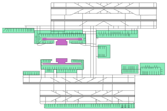
Figure 1.
Runway and taxiway structure at Pudong Airport.
3.2. Data Preprocessing
The flight data in this paper mainly come from the Airport Collaborative Decision Making (A-CDM) system of Pudong airport, where there are some outliers and missing values. Therefore, an upward filling method is used for flights with missing data such as runway numbers. All data with taxiing time less than 0 and exceeding three times the standard deviation are removed, and all numerical features are standardized. As a result, there are 35,037 remaining departure flights.
4. Methodology
In this paper, the K-prototype clustering method is adopted to classify and form typical scenario sets. Subsequently, two adaptive matching methods for scenarios are proposed based on the result of scenario classification. Additionally, the matched target scenario data will then be combined with the pre-trained taxiing time prediction models corresponding to their respective scenario sets. The above processes constitute a taxiing time prediction method based on adaptive scenario matching rules. The process is illustrated in Figure 2.
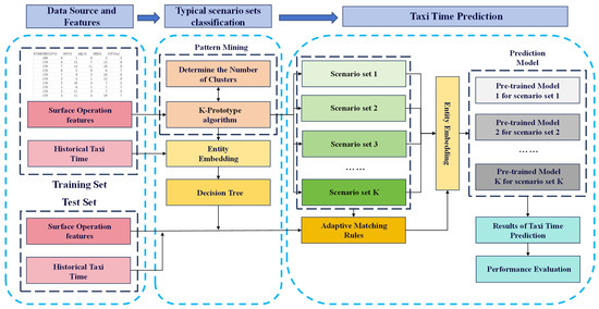
Figure 2.
Taxiing time prediction process based on an adaptive scenario matching method.
4.1. Taxiing Scenario Feature Set Construction
Before determining the scenario classification method and constructing the adaptive matching and prediction process, it is necessary to comprehensively analyze and extract the key factors that affect the taxiing time of departure flights. In order to quantitatively analyze the potential influencing factors, this paper establishes a taxiing scenario feature set based on existing research and the actual operational patterns during the taxiing process for departures. This feature set is based on three aspects: inherent aircraft condition (IAC) features, surface operation environmental (SOE) features, and weather environmental (WET) features.
4.1.1. Inherent Aircraft Condition (IAC) Features
Inherent aircraft condition features refer to the characteristics determined by the flight’s aircraft type and its location. These features include flight number, airline, aircraft type, stand/gate and others. In this study, a total of 15 common features are introduced, namely flight number (), flight mission (), aircraft type (), airline (), departure runway (), destination airport (), runway gate group (), stand/gate (), stand/gate type (), apron (), engine type (), flow control status (), day (), hour (), and minute (). It should be noted that all 15 features are categorical and require additional processing before model training. Due to the lack of taxiing trajectory data, it is considered that aircraft usually select one of several fixed taxiing routes, so this study uses the pairing of runway and parking position to reflect the taxiing distance.
4.1.2. Surface Operation Environmental (SOE) Features
SOE features refer to the estimated traffic situation characteristics during the taxiing process of departure aircraft. These features primarily reflect the potential interactions between the target departure aircraft and other departure or arrival aircraft. Based on the author’s previous research on airport surface movement [13], eight traffic features based on spatiotemporal network topology structures were used. These features comprehensively consider the relationships between departure or arrival flights, as shown in Figure 3. In the figure, the behaviour of flights between the runway and stand/gate and the relationships between aircraft are visualized. Dref represents the target departure aircraft, An represents an arrival aircraft, and Dn represents other departure aircraft. In the subsequent description, we will use this image to provide examples of the calculation methods for each indicator to facilitate understanding. It should be noted that the figure is for illustrative purposes only, representing the possible relationships between flights, and the actual taxiing pattern is not unique.
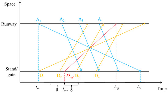
Figure 3.
Ground movement distribution diagram of target flight and arriving flight.
(1) The Scenario Instantaneous Flow Index (SIFI) represents the number of arriving or departure aircraft taxiing on the field when the target aircraft is going to push back. Specifically, SIFI1 () indicates the number of departure aircraft taxiing, while SIFI2 () indicates the number of arrival aircraft taxiing. The calculation method is as follows:
In the equations, denotes whether the -th departure aircraft is in the target interval, denotes whether the -th arrival aircraft is in the target interval, represents the taxiing start time of the arrival aircraft, represents the landing time of the arrival aircraft, represents the taxiing start time of the departure aircraft, and represents the take-off time of the departure aircraft. In the figure, both the SIFI1 and SIFI2 for departure aircraft are 2, including D1, D2, A1, and A2.
(2) The Scenario Cumulative Flow Index (SCFI)
When the target aircraft Dref is taxiing, the scenario cumulative flow index (SCFI) represents the number of departing and arrival aircraft that are also in the taxiing state. Specifically, SCFI1 () indicates the number of departing flights, while SCFI2 () indicates the number of arriving flights. The calculation method is as follows:
All flights in the figure meet the required condition, so the values of SCFI1 and SCFI2 are both 4.
(3) The aircraft queue length index (AQLI) represents the total number of take-off and landing aircraft during the taxiing process of the target aircraft Dref. It is divided into two components: the total number of take-off aircraft, AQLI1 (), and the total number of landing aircraft, AQLI2 (). The calculation method is as follows:
In the figure, the values of AQLI1 and AQLI2 are both 2, including D2, D3 for AQLI1 and A3, A4 for AQLI2.
(4) The Slot Resource Demand Index (SRDI) represents the total number of aircraft that depart from or land on within a time window of δ before and after the push back time of the target aircraft Dref. It consists of two components: the number of departure aircraft, SRDI1 (), and the number of landing aircraft, SRDI2 (). The calculation method is as follows:
In the figure, SRDI1 is 2 and SRDI2 is 1, including D2, D3 for SRDI1 and A2 for SRDI2. Based on relevant research and empirical judgment [11,13], the value of δ is set to 15 min.
All 8 features mentioned above are numerical features. It is important to note that, considering subsequent operational and tactical actions, the estimated departure time and planned take-off time are used when calculating these features. Research [10,11] and subsequent experimental results have shown that this approach can achieve the desired prediction accuracy.
4.1.3. Weather Environmental (WET) Features
During the taxiing process of flights at an airport, they are influenced by numerous environmental factors. However, due to data limitations, this study primarily focuses on using weather conditions as the weather environmental features that impact the taxiing process. This study adopts the Air Traffic Management Performance (ATMAP) weather algorithm [26] proposed by Eurocontrol to simplify the representation of the environmental conditions. This algorithm provides a comprehensive reflection of the meteorological conditions at the airport. A higher value of ATMAP () indicates poorer meteorological conditions at the airport. In addition to ATMAP, the study also includes temperature (), dew point (), visibility (), cloud base height (), wind speed (), cloud density (), thunderstorm conditions (), wind direction (), and gust () as environmental features. These features were not involved in the calculation of ATMAP and were considered separately. Therefore, there are a total of 10 features in the environmental feature set. , , , and are numerical features. , , , and are categorical features.
4.2. Taxiing Scenario Feature Selection
In this study, correlation analysis is applied to select the most critical features that affect taxiing time. However, there are two types of features involved in this study, namely categorical features and numerical features. Considering the different types of features, a single correlation evaluation metric is considered insufficient. Therefore, this study adopts Cramer’s V coefficient, Pearson’s correlation coefficient, and the sample correlation ratio to analyze the correlations between categorical features, numerical features, and the correlation between categorical and numerical features. In addition, partial correlation analysis is used to differentiate whether the correlation between two variables is influenced by a third variable.
- Cramer’s V Coefficient
The Cramer’s V coefficient is used to describe the correlation between two categorical variables. It ranges from 0 (no association between variables) to 1 (complete association). A value of 1 is only achieved when one variable is completely determined by the other. The calculation method is as follows:
and are two categorical variables. Variable has categories, and variable has categories. The number of samples in which category of variable and category of variable coexist is denoted as , while represents the total number of samples. The chi-square statistic is calculated as follows:
In the expression, represents the number of categories for variable , and represents the number of categories for variable . The calculation method for Cramer’s V can be expressed as follows:
In the expression, represents the Phi coefficient, which is formed by dividing the chi-square statistic by the total number of samples.
- Pearson’s Correlation Coefficient
Pearson’s correlation coefficient is a commonly used measure to quantify the linear correlation between two sets of numerical variables. It ranges from −1 to 1, where negative values indicate a negative correlation trend between the variables, and positive values indicate a positive correlation trend.
and are considered two sets of numerical variables, with mean values and . represents the total number of samples. The Pearson’s correlation coefficient is defined as the covariance between the two variables divided by the product of their standard deviations:
- Sample Correlation Ratio
The sample correlation ratio is a measure used to quantify the non-linear relationship between variables based on their statistical deviations. It is defined as the ratio of the statistical deviations representing different categories of a categorical variable. represents the set of categories, and is one of the category elements. represents the number of samples belonging to the category . represents the numerical value corresponding to the category , represents the mean value of the numerical variable for category , and is the weighted average of the mean values of the numerical variable for different categories. The calculation is as follows:
The calculation method for the sample correlation ratio is as follows:
The sample correlation ratio takes values between 0 and 1, where indicates no significant correlation between a categorical variable and a numerical variable, while indicates a significant correlation between them.
- Partial Correlation Analysis
Partial correlation analysis is used to examine the correlation between two variables while controlling for the influence of a third variable. The calculation process for partial correlation analysis is as follows:
- (1)
- The calculation of partial correlation coefficient
There are three variables , with the target variable for correlation analysis being . The partial correlation coefficient is calculated by controlling variable :
where is the correlation coefficient between variable , is the correlation coefficient between variable , and is the correlation coefficient between variable .
- (2)
- Hypothesis testing
To determine whether there is a significant partial correlation between two samples, the calculation method is as follows:
- : The partial correlation coefficient between and is 0.
- : The partial correlation coefficient between and is not 0.
The calculation method for the test statistic is as follows:
where is the partial correlation coefficient, is the sample size, and is the order of partial correlation. The test statistic follows a distribution with degrees of freedom , allowing us to determine whether there is a significant correlation between and at a significance level of .
In summary, the mentioned correlation evaluation indicators will be used for feature selection to construct a taxiing feature set.
4.3. Scenario Classification Based on K-Prototype
The classification of typical scenario sets is an important step in taxi time prediction based on the theory of similar scenarios. This process is important for reducing data heterogeneity and providing effective historical scenario experience references. Therefore, the K-prototype algorithm was adopted in this study with the consideration of mixed-type features.
K-prototype is a clustering method used to address the problem of mixed-type features. It is an improvement on the combination of the K-means and K-mode algorithms [27]. The main process of the K-prototype method is as follows:
The K-prototype algorithm is applied to cluster a dataset , where the -th sample is represented as . The dataset has features, with the first features being numerical features, , and the -th to the -th features being categorical features, . When calculating the dissimilarity between samples, the K-prototype algorithm uses Euclidean distance for the numerical part and Hamming distance for the categorical part. The dissimilarity formula is as follows:
where .
is used to calculate the Euclidean distance between and (the numerical features), is used to calculate the Hamming distance between and (the categorical features), and is the weight for the categorical features. Its value is used to control the balance between categorical and numerical features, preventing a bias towards a specific type of feature. According to the related research [27], the value of depends on the standard deviation (σ) of the numerical features. In this paper, we select 0.5σ as the corresponding value for . The algorithm steps are as follows:
Step 1: Initialize the data by selecting initial cluster centres.
Step 2: Calculate the distances between each sample and the cluster centres using the dissimilarity formula, and assign each sample to the cluster whose centre is closest in distance.
Step 3: Re-evaluate the cluster centres. For the clusters formed in Step 2, calculate the mean for numerical feature clusters and the most frequent value for categorical attribute clusters. These values are then used as the new cluster centres .
Step 4: Calculate the sum of squared errors (SSE). represents cluster , and represents the centroid of cluster . The SSE is defined as follows:
After calculating the SSE for rounds of clustering, the calculation stops when is reached. represents the stopping threshold. Otherwise, return to Step 2.
The scenario classification results obtained through the K-prototype process will be applied as typical scenario sets for adaptive matching rules and taxiing time prediction.
4.4. Taxiing Time Prediction Based on Adaptive Matching Rules
According to the taxiing time prediction process, the scenario in which the target flight is located should be matched to a certain typical scenario set. This process needs to follow a quantitative matching rule, so the adaptive matching method is considered for scenario matching in this paper.
The adaptive matching method used in this paper primarily relies on a decision tree (DT) classifier with scenario labels obtained from clustering as the supervised condition. The parameters from the trained DT classifier model are used for adaptive matching rules. There are two adaptive matching methods adopted in this paper, named ‘scenario matching rules based on decision tree pruning strategy’ and ‘scenario matching rules based on complexity’:
- (1)
- Scenario matching rules based on decision tree pruning strategy: According to the training results of the decision tree, all branch conditions with high feature importance are extracted and pruned [28,29] to make quantitative matching rules for different similar scenario sets. This strategy allows for a relatively straightforward acquisition of matching rules for different scenario sets. However, it is important to note that due to the limitation of feature types, this rule only uses numerical features as branch conditions. In the implementation process, firstly, categorical features require additional entity embedding processing to achieve a reduction in the dimensionality of high-dimensional vectors and reduce consumption of computational resources. Afterwards, for each branching node, the most important feature based on the importance of numerical features within the node is selected as the branching condition. It should be noted that due to the multitude of branching results, additional pruning and consolidation [28,29] are required to generate threshold values that are easy to use. Ultimately, a comprehensive set of scenario matching rules is formed.The process is shown in Algorithm 1.
Algorithm 1: Scenario matching rules based on decision tree pruning strategy Input: Scenario training data (including set labels) , where represents categorical features, represents numerical features, represents scenario labels and represents the total number of scenarios in the training set. Output: Scenario matching rules 1: Entity embedding and normalized categorical features. The processed features are . 2: Training of a DT classifier model 3: Extraction of the branch conditions of the most critical features for each node. 4: Pruning of the branch conditions and integration with the smallest loss of precision to obtain the scenario matching rules . 5: Return Scenario matching rules - (2)
- Scenario matching rules based on complexity: Due to the high number of categorical features involved in this paper, it is difficult to directly design adaptive matching rules based on scenario sets. Therefore, this paper proposes two evaluation metrics, namely “scenario complexity” and “departure–arrival scenario complexity deviation”, for the process of adaptive scenario matching. These metrics are calculated based on the scenario classification data obtained from clustering. The importance weights of various features obtained from the DT classification model are used in the process of calculating complexity. The calculation process is as follows:where represents the importance of the -th feature in the decision tree, derived from Gini importance and mean impurity reduction. represents the value of the feature in the scenario . represents the traffic feature set, composed of and . represents the departure traffic feature set, including SCFI1 and AQLI1. represents the arrival traffic feature set, including SCFI2 and AQLI2.
The calculation process is as follows: Firstly, similar to the first method, the categorical features require additional entity embedding processing. Secondly, based on the decision tree training results, the importance of all features is calculated with metrics such as Gini importance and mean impurity reduction. The thresholds for distinguishing between scenarios are computed for each feature with the importance calculation results. Finally, the complexity values with the highest scenario division accuracy are used as the threshold for branching scenario sets. The threshold is calculated by taking a step size of 0.01 and the complexity values with the highest accuracy in scenario division between each pair of scenario sets are selected as the boundary threshold for sets. Finally, the threshold results between each pair of scenarios are merged and pruned to form the adaptive matching rules. The process is shown in Algorithm 2.
| Algorithm 2: Scenario matching rules based on complexity |
| Input: Scenario training data (including set labels) , where represents categorical features, represents numerical features, represents scenario labels and represents the total number of scenarios in the training set. |
| Output: Scenario matching rules |
| 1: Entity embedding and normalized categorical features. The processed features are . |
| 2: Training of a DT classifier model |
| 3: Calculation of the importance of all features based on Gini importance and mean impurity reduction. |
| 4: Calculation of the scenario complexity for each scenario in |
| 5: Calculation of the departure–arrival scenario complexity deviation for each scenario in |
| 6: Calculation of the threshold boundary between each pair of scenario sets. |
| 7: Integration of the boundary results to form scenario matching rules |
| 8: Return Scenario matching rules |
In summary, the taxiing time prediction process will be based on the results of the two adaptive matching rules. The prediction model with the smallest error for each typical scenario set will be combined with the adaptive matching process to form the taxiing time prediction method based on similar scenarios.
4.5. Entity Embeddings
To reduce the computational cost of the adaptive matching process and subsequent predictions, entity embedding is used to process categorical features [30]. Entity embedding has been widely used in Natural Language Processing (NLP) research. Compared to traditional one-hot encoding, entity embedding not only improves storage space utilization and computational efficiency but also captures the underlying relationships between categorical features through the mapped values.
Entity embedding is implemented using supervised learning. There is a categorical feature with kinds of feature categories. The category of the feature , denoted as , can be mapped to a one-hot encoded vector ., which is a vector of length .
In the one-hot vector , the element at the position representing a certain category can be denoted as .The element is non-zero only when the represented types of and are the same in the vector , while the rest of the elements are zeros. After feeding the encoded one-hot vector into a neural network under supervised learning, the output given the input is defined as follows:
where represents the weights connecting the one-hot encoding layer and the embedding layer, represents the input to the embedding layer, and represents the dimension of the embedding layer. Similarly, a neural network under the corresponding supervised condition can be formed by adding a set of fully connected layers after the embedding layer. This allows for obtaining the weights of all categorical features in the embedding layer and using them as the values for each category. After extraction, the categorical features are merged with numerical features to form the dataset for the matching and prediction.
5. Experiments
The computer configuration used in this study includes a CPU: Core i9-13900HX, 64 GB RAM, and an NVIDIA 4060 graphics card (Santa Clara, CA, USA). The entire computational process was carried out using the Python programming language (version 3.10).
5.1. Adaptive Scenario Matching Results
5.1.1. Taxiing Scenario Feature Selection Results
Correlation analysis was conducted using a total of 33 features mentioned in Section 4.2 and the correlation evaluation indicators from Section 4.1. The results of the relationship between features are shown in Figure 4, which indicates significant correlations among certain features in IAC, SOE, and WET.
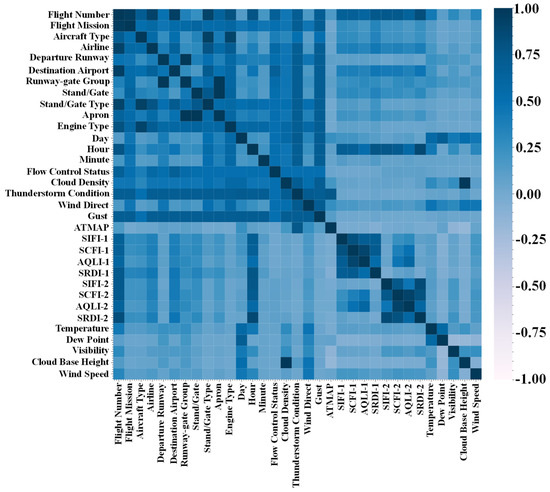
Figure 4.
Heatmap of feature correlation analysis.
Additionally, as shown in Table 1 and Figure 5, the correlation analysis was used between each feature and the taxiing time. Key features were selected based on the Pearson correlation coefficient or sample correlation ratio between the features and taxiing time. Furthermore, partial correlation analysis was used to examine the relationship between numerical features and taxiing time, with a confidence level set at 0.05. It is important to note that in Table 1, when the p-value is shown as 0, it does not indicate an actual value of 0. The reason for this is that the computed result is extremely small, so it is approximated as 0.

Table 1.
Results of the correlation analysis of numerical features and taxiing time.
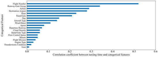
Figure 5.
Results of correlation analysis of categorical features and taxiing time.
According to the analysis results, the feature selection process is as follows. All features with correlation coefficients less than 0.2 with taxiing time are removed. If there is a high correlation (more than 0.7) between categorical features, the features with higher correlation with taxiing time are retained. The processed features are presented in Table 2; there are a total of nine, including five categorical features and four numerical features. It can be observed that the correlation between weather features and taxiing time is relatively weak, with almost no correlation between taxiing time and other weather features except for wind direction.

Table 2.
Processed key feature set.
The key feature set mentioned above is used for subsequent scenario classification, adaptive matching rules, and the taxiing time prediction process.
5.1.2. Scenario Classification and Scenario Adaptive Matching Results
As shown in Figure 6, this paper adopts a combination of the elbow method and silhouette coefficient to analyze the optimal number of clusters. The optimal number of clusters is determined to be four with the K-prototype algorithm.
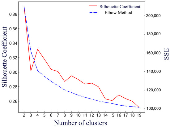
Figure 6.
Evaluation indicators for the optimal number of clusters.
The number of flights in the four generated scenario sets is as follows: 6834 flights, 11,165 flights, 6008 flights, and 11,030 flights. In Figure 7 and Figure 8, partial clustering results are presented, and significant differences can be observed among different sets. In Scenario set 1, flights are primarily departures with a higher occurrence during the morning and noon peaks. In Scenario set 2, flights are mainly arrivals and are primarily distributed throughout the afternoon and evening. Scenario set 3 has the longest average taxiing time and is concentrated during the morning and noon peaks. Scenario set 4 has the lowest number of flights and is distributed throughout the day The flights in this scenario set are concentrated on the third apron (freight apron), with a predominance of medium to large aircraft types. The number of flights on the surface involved in each scenario in this set is significantly smaller than the other three sets. Additionally, the flights in the scenarios mainly consist of cargo flights. The probability density distribution of taxiing time for each scenario set is shown in Figure 9. The taxiing time distributions in Scenario sets 1 and 2 are similar, while Scenario set 3 exhibits a wider range of values, and the taxiing times in Scenario set 4 are concentrated at lower values.
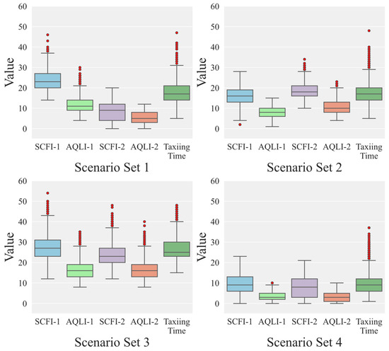
Figure 7.
Boxplot of features in different scenario sets.
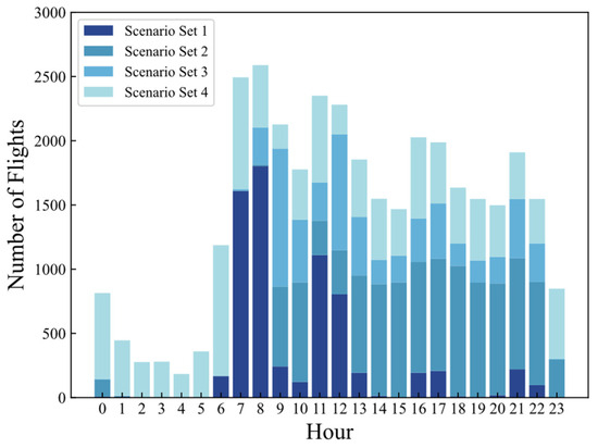
Figure 8.
Hour distribution of different scenario sets.
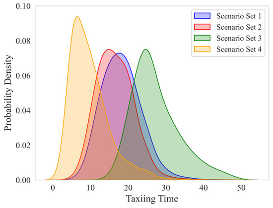
Figure 9.
Probability distribution of taxiing time.
Therefore, this paper defines various scenario sets as follows: Scenario set 1 represents departure peak scenarios, Scenario set 2 represents arrival peak scenarios, Scenario set 3 represents arrival–departure peak scenarios, and Scenario set 4 represents other scenarios.
In the actual prediction process, it is necessary to match the current scenario of the flight with the typical scenario sets in order to select the corresponding pre-trained model for taxi time prediction. This matching process refers to the results of scenario classification and combines the matching methods in Section 4.4 for analysis.
First, a DT classifier will be built to reflect the matching process for the similar scenarios. The labels of the scenario sets are used as the supervised condition, with 80% of the data used for training and 20% for testing. Ten-fold cross-validation is used for parameter optimization. Furthermore, entity embedding is used for categorical features in this process. It can compress the 16,842-dimensional vectors to 250 dimensions, which significantly reduces the training cost.
The recall, precision, F1 score, and specificity metrics are calculated for the matching results, as shown in Table 3. Across the four scenario sets, all evaluation indicators maintain a level above 90%. Meanwhile, branches and feature importance are provided by constructing this decision tree for rule formulation.

Table 3.
Adaptive matching results for different scenario sets.
Finally, the scenario matching rules of the two method mentioned in Section 4.4 are shown in Table 4. On one hand, the result of scenario matching rules based on the decision tree pruning strategy is shown in Figure 10. This paper only prunes and summarizes 5727 nodes in the decision tree using numerical features [28,29] for practical application in operational control processes. The partition rules are sampled for verification, and the results show an accuracy of 82.2% for these rules.

Table 4.
Matching rules for different scenario sets.
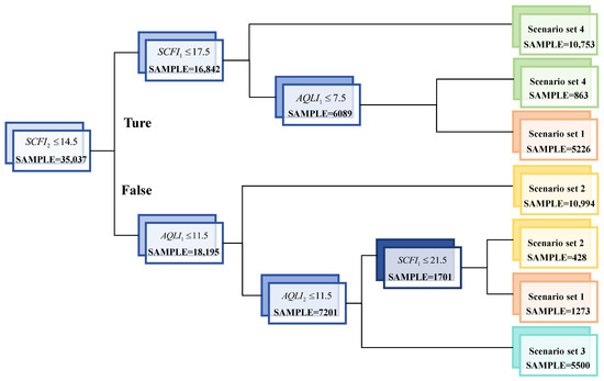
Figure 10.
The result of scenario matching rules based on the decision tree pruning strategy.
On the other hand, the results of scenario matching rules based on complexity are shown in Figure 11. The results demonstrate that this matching method with complexity can effectively differentiate different scenario sets. However, it is evident that scenario set 1 and set 2 cannot be matched well. Therefore, is considered to distinguish the differences between scenario set 1 and scenario set 2, which are difficult to distinguish, and the result is shown in the right-hand graph of Figure 11. The results indicate that can effectively differentiate between the two scenario sets.
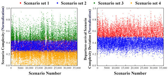
Figure 11.
Results of complexity for different scenario sets.
The complexity thresholds in this method are provided in Figure 12, where the two red lines correspond to the significant boundaries observed in the left-hand graph of Figure 11. The calculation method of involves the peak value of the highest division accuracy between adjacent different scenario sets and taking the average of the two boundaries on the same side. As for , the value of the highest accuracy is directly extracted. According to the results obtained from the test set, the overall accuracy of this method is 85.3%. It can ensure a relatively high level of accuracy in scenario matching.
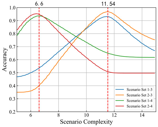
Figure 12.
Distribution of matching accuracy and boundary threshold for different scenario sets.
In summary, the accuracy results of the above two scenario adaptive matching methods indicate that both can achieve satisfactory outcomes. The actual airport operational control units can choose the appropriate matching rules according to their needs. In the subsequent sections of this paper, scenario matching rules based on complexity will be used to predict taxiing times.
5.2. Prediction Results and Discussion
5.2.1. Taxiing Time Prediction Results
This paper compares the pre-trained performance of taxi time prediction models for various scenario sets. This study adopted six different prediction models for predicting taxiing time and made a comparison among these models: multivariable linear regression (MLR), decision tree (DT), support vector regression (SVR), random forest regression (RF), gradient boosting regression trees (GBRT), and multilayer perceptron (MLP). The optimal prediction model was selected based on obtained results.
During the taxiing time prediction process, the prediction accuracy of six different models was compared for the four scenario sets in Section 5.1.2. Six indicators were used to evaluate the accuracy of taxiing time predictions: MAE (mean absolute error), RMSE (root mean square error), R-squared (R2), accuracy within one minute, accuracy within three minutes, and accuracy within five minutes.
The results, as shown in Figure 13, illustrate the cumulative error distribution of taxiing time prediction for each scenario set. Among all the methods, it can be observed that the accuracy of prediction is highest for the departure peak scenario. However, there is a larger deviation in the prediction results for the arrival–departure peak scenario. This is because the departure peak scenarios occur in a more concentrated manner, with a relatively homogeneous mix of flight types. Higher accuracy can be achieved due to the simpler scenarios. On the other hand, the arrival–departure peak scenarios involve a diverse range of flight types and complex coupling between arrivals and departures. This makes taxiing time prediction challenging within these scenarios.
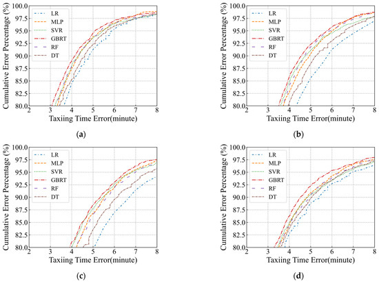
Figure 13.
Prediction results of different scenario sets. (a) Departure peak scenarios. (b) Arrival peak scenarios. (c) Arrival–departure peak scenarios. (d) Other scenarios.
In terms of method, the overall prediction performance of different models across all scenarios is considered, as shown in Table 5. The GBRT model performed exceptionally well in all scenario sets. The MLP model achieved prediction results second only to GBRT, further highlighting the superiority of nonlinear models. Additionally, random forest and GBRT produced better results compared to DT and other methods, demonstrating the advantages of ensemble learning paradigms. This conclusion aligns with previous research [11,31] and demonstrates the validity of the test results.

Table 5.
Performance of different models in all scenarios.
5.2.2. Overall Performance Evaluation
In this section, a comparison is made between the proposed hybrid machine learning model and six other baseline methods. It is important to note that these baseline methods do not involve scenario classification and adaptive matching rules for the overall prediction process. The results are shown in Table 6. Compared to the baseline model using one-hot encoding, the GBRT model based on adaptive matching rules achieved a 4.8% decrease in MAE and a 12.6% decrease in RMSE for the optimal prediction results.

Table 6.
Comprehensive performance of different prediction models.
This process significantly reduces the fluctuations caused by data heterogeneity. However, it is important to note that the interpretability of entity embedding methods is currently limited, and they cannot effectively explain the reasons for the relationships between variables. This issue needs to be addressed in future research.
5.2.3. Feature Importance Analysis for Different Scenario Sets
Feature importance is calculated through the taxiing time prediction process for each scenario set. Further analysis can be conducted to identify the key factors influencing taxiing time by ranking them in different scenario sets. As shown in Figure 14, it can be concluded that among the features of various scenarios, the variables hour, AQLI1, and AQLI2 generally have higher importance than other features. However, the ranking of feature importance also varies depending on the scenario sets. For example, in the departure peak scenario set, AQLI1 is the most critical feature, while in the arrival peak scenario set, the most critical feature is AQLI2. This is the same as the actual operational experience.
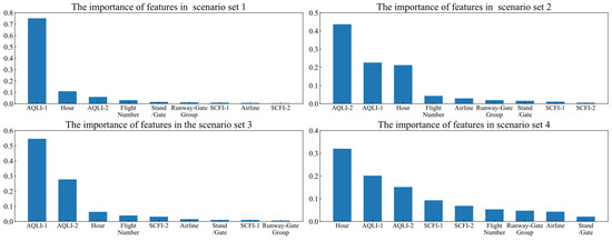
Figure 14.
Feature importance in different scenario sets.
The above analysis indicates that the method proposed in this paper can not only enhance the attention of the predictive model to key features in different scenarios, reducing the impact caused by data heterogeneity, but can also verify the effectiveness of the selected taxiing scenario feature set in describing taxiing scenarios. Therefore, this method is a valid method of improving fine-grained control on the airport surface.
6. Conclusions
In research on airport surface operational control, accurate taxi time prediction and the effective guidance of surface operations through decisions made by air traffic controllers in historical scenarios have always been important research topics. In this article, we propose a taxi time prediction method that incorporates scenario classification and adaptive matching rules. This method generates multiple typical taxiing scenario sets and reduces prediction errors for taxiing time in each of these scenario sets. The main conclusions of this paper are as follows:
- (1)
- In this paper, a heterogeneous feature set for taxiing scenarios is proposed, and the key feature selection process incorporates various correlation analysis indicators. According to the correlation analysis results, nine features that are most relevant to taxiing time have been identified. In addition, when combined with the prediction outcomes of the model, AQLI1, AQLI2, and hour of the day make significant contributions to taxiing time prediction across various scenario sets, while environmental features such as weather conditions have a relatively low correlation with taxiing time. These results confirm the effectiveness of the selected feature set.
- (2)
- Furthermore, two adaptive matching methods are proposed for flight operation scenarios based on K-prototype, which generates four sets of scenarios: departure peak scenarios, arrival peak scenarios, arrival–departure peak scenarios, and other scenarios. The recognition accuracies of the two adaptive matching methods for similar scenarios are 82.2% and 85.3%. Both of these methods maintain high accuracy, and this result has strong operability. Airport operations departments can select the appropriate adaptive matching method based on their actual needs.
- (3)
- This paper proposes a taxiing time prediction method based on adaptive scenario matching rules. The method demonstrates a reduction of 4.8% and 12.6% in MAE and RMSE with the data from Pudong Airport when compared to baseline methods. The results indicate that this method significantly reduces the volatility of prediction results caused by data heterogeneity. It can provide support for the formulation of surface traffic control strategies during actual operations and act as a feasible decision making aid.
In future work, firstly, we aim to integrate this method with the aircraft surface operations control process to develop a more reasonable aircraft departure plan and analyze its contribution to reducing carbon emissions and mitigating environmental pollution. Secondly, to achieve more accurate predictions, we will further test the relationship between additional influencing factors and the model’s predictive performance and incorporate more advanced evaluation indicators. Lastly, current research lacks analysis of model performance and results under extreme weather conditions or when critical airport facilities are unavailable (for example, during runway closures, pavement maintenance, etc.). We will conduct comprehensive analyses of airports that meet the aforementioned conditions to assess the model’s capacity for generalization.
Author Contributions
Conceptualization, P.Q.; Methodology, P.Q.; Software, P.Q. and M.Y.; Validation, J.S.; Investigation, Y.C.; Resources, M.H.; Data curation, M.H. and M.Y.; Writing—review & editing, J.Y.; Visualization, J.S.; Supervision, J.Y. All authors have read and agreed to the published version of the manuscript.
Funding
This work was funded by the National Key R&D Program of China (No. 2021YFB1600500), the National Natural Science Foundation of China (No. 52002178) and the Natural Science Foundation of Jiangsu Province (Grant No. BK20190416).
Data Availability Statement
The raw data supporting the conclusions of this article will be made available by the authors on request.
Acknowledgments
We would like to thank the State Key Laboratory of Air Traffic Management System for providing the data used in the model tests described in this paper.
Conflicts of Interest
The authors declare no conflicts of interest.
References
- EUROCONTROL. Airport Collaborative Decision-Making [EB/OL]. Available online: https://www.eurocontrol.int/concept/airport-collaborative-decision-making (accessed on 1 June 2023).
- Postorino, M.N.; Mantecchini, L.; Paganelli, F. Improving taxi-out operations at city airports to reduce CO2 emissions. Transp. Policy 2019, 80, 167–176. [Google Scholar] [CrossRef]
- Khammash, L.; Mantecchini, L.; Reis, V. Micro-simulation of airport taxiing procedures to improve operation sustainability: Application of semi-robotic towing tractor. In Proceedings of the 2017 5th IEEE International Conference on Models and Technologies for Intelligent Transportation Systems (MT-ITS), Napoli, Italy, 26–28 June 2017; pp. 616–621. [Google Scholar]
- Zaninotto, S.; Gauci, J.; Zammit, B. An Autonomous Tow Truck Algorithm for Engineless Aircraft Taxiing. Aerospace 2024, 11, 307. [Google Scholar] [CrossRef]
- Jiang, Y.; Wang, Y.; Xue, Q.; Wu, W. Research on Space-Time Taxiing Optimization of Aircraft Based on Carbon Emission, Huanan Ligong Daxue Xuebao. J. South China Univ. Technol. Nat. Sci. 2023, 51, 152–159. [Google Scholar] [CrossRef]
- Postorino, M.N.; Mantecchini, L.; Gualandi, E. Integration between aircraft and handling vehicles during taxiing procedures to improve airport sustainability. Int. J. Transp. Dev. Integr. 2016, 1, 28–42. [Google Scholar] [CrossRef]
- Di Mascio, P.; Corazza, M.V.; Rosa, N.R.; Moretti, L. Optimization of aircraft taxiing strategies to reduce the impacts of landing and take-off cycle at airports. Sustainability 2022, 14, 9692. [Google Scholar] [CrossRef]
- Chen, Y.; Luh, P.B.; Guan, C.; Zhao, Y.G.; Michel, L.; Coolbeth, M.; Friedland, P.; Rourke, S.J. Short-term load forecasting: Similar day-based wavelet neural networks. IEEE Trans. Power Syst. 2009, 25, 322–330. [Google Scholar] [CrossRef]
- Son, J.; Cha, J.; Kim, H.; Wi, Y.M. Day-ahead short-term load forecasting for holidays based on modification of similar days’ load profiles. IEEE Access 2022, 10, 17864–17880. [Google Scholar] [CrossRef]
- Jiang, Z.; Zhang, L.; Ji, T. NSDAR: A neural network-based model for similar day screening and electric load forecasting. Appl. Energy 2023, 349, 121647. [Google Scholar] [CrossRef]
- Du, J.; Hu, M.; Zhang, W.; Yin, J. Finding Similar Historical Scenarios for Better Understanding Aircraft Taxi Time: A Deep Metric Learning Approach. IEEE Intell. Transp. Syst. Mag. 2022, 15, 101–116. [Google Scholar] [CrossRef]
- Clewlow, R.; Simaiakis, I.; Balakrishnan, H. Impact of arrivals on departure taxi operations at airports. In Proceedings of the AIAA Guidance, Navigation, and Control Conference, Toronto, ON, Canada, 2–5 August 2010; p. 7698. [Google Scholar]
- Yin, J.; Hu, Y.; Ma, Y.; Xu, Y.; Han, K.; Chen, D. Machine learning techniques for taxi-out time prediction with a macroscopic network topology. In Proceedings of the 2018 IEEE/AIAA 37th Digital Avionics Systems Conference (DASC), London, UK, 23–27 September 2018; IEEE: Piscataway, NJ, USA, 2018; pp. 1–8. [Google Scholar]
- Wang, X.; Brownlee, A.E.; Woodward, J.R.; Weiszer, M.; Mahfouf, M.; Chen, J. Aircraft taxi time prediction: Feature importance and their implications. Transp. Res. Part C Emerg. Technol. 2021, 124, 102892. [Google Scholar] [CrossRef]
- Ravizza, S.; Atkin, J.A.; Maathuis, M.H.; Burke, E.K. A combined statistical approach and ground movement model for improving taxi time estimations at airports. J. Oper. Res. Soc. 2013, 64, 1347–1360. [Google Scholar] [CrossRef]
- Lordan, O.; Sallan, J.M.; Valenzuela-Arroyo, M. Forecasting of taxi times: The case of Barcelona-El Prat airport. J. Air Transp. Manag. 2016, 56, 118–122. [Google Scholar] [CrossRef]
- Idris, H.; Clarke, J.P.; Bhuva, R.; Kang, L. Queuing Model for Taxi-Out Time Estimation; MIT: Cambridge, MA, USA, 2001. [Google Scholar]
- Jordan, R.; Ishutkina, M.A.; Reynolds, T.G. A statistical learning approach to the modeling of aircraft taxi time. In Proceedings of the 29th Digital Avionics Systems Conference, Salt Lake City, UT, USA, 3–7 October 2010; IEEE: Piscataway, NJ, USA, 2010; pp. 1. B. 1-1–1. B. 1-10. [Google Scholar]
- Ravizza, S.; Chen, J.; Atkin, J.A.; Stewart, P.; Burke, E.K. Aircraft taxi time prediction: Comparisons and insights. Appl. Soft Comput. 2014, 14, 397–406. [Google Scholar] [CrossRef]
- Chen, J.; Weiszer, M.; Zareian, E.; Mahfouf, M.; Obajemu, O. Multi-objective fuzzy rule-based prediction and uncertainty quantification of aircraft taxi time. In Proceedings of the 2017 IEEE 20th International Conference on Intelligent Transportation Systems (ITSC), Yokohama, Japan, 16–19 October 2017; IEEE: Piscataway, NJ, USA, 2017; pp. 1–5. [Google Scholar]
- Balakrishna, P.; Ganesan, R.; Sherry, L. Accuracy of reinforcement learning algorithms for predicting aircraft taxi-out times: A case-study of Tampa Bay departures. Transp. Res. Part C: Emerg. Technol. 2010, 18, 950–962. [Google Scholar] [CrossRef]
- Murça, M.C.R. A robust optimization approach for airport departure metering under uncertain taxi-out time predictions. Aerosp. Sci. Technol. 2017, 68, 269–277. [Google Scholar] [CrossRef]
- Lian, G.; Zhang, Y.; Desai, J.; Xing, Z.; Luo, X. Predicting taxi-out time at congested airports with optimization-based support vector regression methods. Math. Probl. Eng. 2018, 2018, 7509508. [Google Scholar] [CrossRef]
- Lee, H.; Malik, W.; Jung, Y.C. Taxi-out time prediction for departures at Charlotte airport using machine learning techniques. In Proceedings of the 16th AIAA Aviation Technology, Integration, and Operations Conference, Washington, DC, USA, 13–17 June 2016; p. 3910. [Google Scholar]
- Diana, T. Can machines learn how to forecast taxi-out time? A comparison of predictive models applied to the case of Seattle/Tacoma International Airport. Transp. Res. Part E Logist. Transp. Rev. 2018, 119, 149–164. [Google Scholar] [CrossRef]
- EUROCONTROL. Algorithm to Describe Weather Conditions at European Airports Brussels: EUROCONTROL. 2009. Available online: https://www.eurocontrol.int/sites/default/files/publication/files/algorithm-met-technical-note.pdf (accessed on 4 June 2024).
- Huang, Z. Clustering large data sets with mixed numeric and categorical values. In Proceedings of the 1st Pacific-Asia Conference on Knowledge Discovery and Data Mining, (PAKDD), Singapore, 23–24 February 1997; pp. 21–34. [Google Scholar]
- An, N. Correlation Analysis of Traffic Accident Factors and Accident Grades; Chang’an University: Xi’an, China, 2021. [Google Scholar] [CrossRef]
- Liu, J.; Xu, X.; Wu, F.; Li, F.; Wang, Y. Quantitative Risk Evaluation of Water Inrush Hazard Based on Decision Tree of Underground Engineering; METAL MINE: Ma’anshan City, China, 2023; pp. 217–224. [Google Scholar] [CrossRef]
- Guo, C.; Berkhahn, F. Entity embeddings of categorical variables. arXiv 2016, arXiv:1604.06737. [Google Scholar]
- Grabbe, S.; Sridhar, B.; Mukherjee, A. Clustering days and hours with similar airport traffic and weather conditions. J. Aerosp. Inf. Syst. 2014, 11, 751–763. [Google Scholar] [CrossRef]
Disclaimer/Publisher’s Note: The statements, opinions and data contained in all publications are solely those of the individual author(s) and contributor(s) and not of MDPI and/or the editor(s). MDPI and/or the editor(s) disclaim responsibility for any injury to people or property resulting from any ideas, methods, instructions or products referred to in the content. |
© 2024 by the authors. Licensee MDPI, Basel, Switzerland. This article is an open access article distributed under the terms and conditions of the Creative Commons Attribution (CC BY) license (https://creativecommons.org/licenses/by/4.0/).