An Engine Deterioration Model for Predicting Fuel Consumption Impact in a Regional Aircraft

Abstract

A deterioration cycle model is presented, designed to consider the turbomachinery efficiency losses that are expected during real engine in-service operations. The cycle model was developed using information from practical experience found in the literature to account for both short- and long-term deterioration effects; the former occurring during the first flight cycles, the latter due to regular in-service operation. This paper highlights the importance of analyzing the inter-turbine temperature margin ($ITTM$) to track engine deterioration to determine the extent of an in-service engine life. The proposed model was used to assess the $ITTM$ and fuel consumption impact in the CRJ-700 regional aircraft (powered by two CF34-8C5B1 engines) for three representative missions: short (0.4 h), average (1.4 h), and long (2.5 h), considering different levels of engine deterioration, from the new engine level up to fully deteriorated. The fuel consumption at the new engine level (zero deterioration) was validated against a real-time engine model embedded in a Level-D flight simulator, the so-called Virtual Research Flight Simulator located at the Laboratory of Applied Research in Active Control, Avionics, and AeroServoElasticity. The errors found in this validation for the trip mission fuel consumption in the short, average, and long missions were −3.6, +0.9, and +0.6%, respectively. The cycle model predictions suggest the $ITTM$ for a new engine is 55.2 °C, whereas for a fully deteriorated engine, it is 26.4 °C. Finally, in terms of fuel consumption, the results presented here show that an average CF34-8C5B1 engine shows an increase in the cumulative fuel consumption of 2.25% during its life in service, which translates to a 4.5% impact in aircraft fuel consumption.

1. Introduction

Fuel consumption in the transportation industry, especially for aviation, has been a controversial topic for the past few years due to the alleged impact on global warming caused by increased greenhouse gas emissions (e.g., CO₂). Assessments made in 2018 estimated aviation emissions as approximately 2.4% of the total anthropogenic (i.e., human-caused) emissions of CO₂ [1].

Significant efforts are underway to decarbonize the aviation industry towards net zero growth beyond 2020 and to reduce emissions to half of those observed in 2005 by 2050 [2]. To achieve this goal, advanced propulsion systems (hybrid electric [3,4,5] and fuel cells [6,7]) and alternative fuels, such as sustainable aviation fuels (SAFs) [8] and hydrogen [8,9,10], are being studied. Concerning the former, it seems their suitability for commercial aircraft is still limited for the foreseeable future until its performance can be made comparable to that of traditional gas turbine engines (GTEs) and conventional aviation fuels (CAFs). Some predictions limit their use to low-speed aircraft carrying a small number of passengers for short-distance flights [11].

In the case of alternative fuels, SAFs seem the best option to achieve the aviation greenhouse emissions reduction targets. SAFs are designed to present little to no disruption to the industry. They exhibit characteristics similar to those of CAFs (in terms of heating value and hydrocarbon ratio) and thus are intended to use the same infrastructure (i.e., storage and distribution) as CAFs, with no modification to the aircraft/engines, hence the term ‘drop-in’ fuel [12]. At the time of writing this paper, most of the flight tests conducted with SAFs have been performed with a combination of CAFs (i.e., kerosene-based fuels) in ratios of up to 50% [13].

Based on the ongoing research and current practices, it seems reasonable to assume that traditional aircraft and engines will be used for a significant time in the future, utilizing combinations of blended fuels, progressing towards 100% SAFs. Even after the aviation industry has fully transitioned to SAFs, fuel consumption will still be the greatest concern for operational efficiency, especially as it is expected that aircraft operated with SAFs will be more expensive, at least until sufficient technology maturation or incentives for producing them more affordably are in place [12].

Aircraft fuel consumption is mainly influenced by both aircraft and engine technology, including their degradation and operational practices. This paper focuses only on the impact caused by engine degradation. Other factors affecting fuel consumption are outside the scope of this work.

GTEs are composed of modules such as compressors and turbines. As an engine accumulates hours in operation (or in service), the internal parts of these components degrade and ultimately cause losses in the components’ adiabatic efficiencies. The adiabatic efficiency ($\eta$) is a well-known performance metric in turbomachinery design; it describes the specific work ($∆h$) conducted in a real vs. an ideal process. A loss of efficiency means that a compressor will require more work to compress the working fluid to the target pressure ratio; conversely, for a turbine, lower efficiency indicates that a lower work output will be produced.

The efficiency losses ($\mathsf{\Delta }\eta$) affect an engine’s specific fuel consumption ($SFC$), a measure of the overall engine efficiency. The $SFC$ is defined as the ratio of the fuel flow rate injected in the combustor (${\dot{m}}_{fuel}$) to the net thrust ($F_n$) produced by the engine (Equation (1)). The net result of the loss of engine efficiency is translated to a greater fuel consumption, which results in both higher operational costs and higher gas emissions.

$$SFC=\frac{{\dot{m}}_{fuel}}{F_n}$$

(1)

In the thermodynamic cycle, the overall effect of having lower component efficiencies is to increase the fuel input and the operational temperatures of the hot section (i.e., downstream of the combustor), one of which is the exhaust gas temperature ($EGT$). Such a loss in efficiency is an expected consequence of the second law of thermodynamics (i.e., increased entropy generation due to aging). Comprehensive discussions of the specific factors of engine deterioration (fouling, corrosion, erosion, abrasion, etc.) are provided in [14,15].

Several deterioration cycle models were found in our literature review. Zaita et al. [15] developed a deterioration model for a military application using a turbomachinery stage-stacking method that modifies the stage characteristics (flow and efficiency) of turbomachinery with values derived from empirical correlations obtained by the US Navy. These correlations allow the deviations from flow and efficiency caused by the deterioration effects (e.g., fouling, erosion) to be determined. The effects due to deterioration at each stage are then stacked to generate the overall impact in the turbomachinery components, which is then input to the cycle model to compute the influence on thrust and $SFC$.

Venediger [16] considered an in-house integrated framework encompassing aircraft, engine thermodynamic and emissions models for assessing the impact in fuel consumption and emissions for a single aisle aircraft Only long-term engine deterioration effects were considered, in which 2.0% efficiency losses in the high-pressure compressor (HPC), combustor, and high-pressure turbine (HPT) were studied. The salient results indicated that between clean and deteriorated engines, an increase in fuel consumption of about 5.0% was observed for a mid-range mission.

Kelaidis et al. [17] used an integrated platform with different sub-models representing aircraft kinematics, an engine model, and emissions. The outcome of this platform provides information about an aircraft’s trajectory and its kinematics, engine parameters (including emissions), and fuel burned. The engine model in the platform was adapted to represent the CFM56-3C1 engine. Their engine degradation assessment was accomplished by examining two cases (considering the same mission), one with new engines and the other with highly degraded engines. The conclusion from this comparison is that the fuel required for an aircraft with degraded engines is 3.5% more than that needed with new engines.

While several deterioration models have been studied by researchers, the most reliable deterioration models are those developed by original engine manufacturers (OEMs). Such models rely on empirical relationships derived during in-service operations. Seminal studies performed by two of the leading North American OEMs are presented by Wulf et al. [18] and Salle [19], assessing the causes of engine deterioration and its impact on performance for the General Electric (GE) CF6-6D and Pratt & Whitney (P&W) JT9D engines, respectively. Accumulating data from different sources, such as performance measurements taken both from the test cell (sea level) and on-wing (during cruise), in addition to hardware inspections and measurements, allowed both references to characterize the average $SFC$ loss during in-service operations.

The first objective of this paper is to use information from practical experience, such as the work in [18], to develop a thermodynamic deterioration model that can predict the increase in average fuel consumption ($f_c$) throughout the life of a regional aircraft engine, namely, the CF34-8C5B1. Moreover, this paper highlights the importance of analyzing the inter-turbine temperature ($ITT$) margin to track engine deterioration to determine the in-service engine life.

The second objective of this research is to assess the $f_c$ on the MHI CRJ-700 (previously Bombardier CRJ-700) aircraft for three representative missions, short (0.4 h), average (1.4 h), and long (2.5 h), considering different levels of engine deterioration.

The salient results reported in [18] were used to develop a thermodynamic model that relates the efficiency loss ($∆\eta$) of each major turbomachinery component (or module) with a normalized time index ($\tau$), designed to represent a measure of the in-service time. The deterioration model was incorporated into the thermodynamic model that represents the CF34-8C5B1, the so-called CM-8C5B1 [20], which predicts the performance under new engine conditions (i.e., no deterioration). The final compound model can predict the performance of the engine throughout its operational life, from new engine (zero deterioration) to fully deteriorated (100% deterioration).

The rest of this paper is arranged as outlined here: Section 2 discusses the importance of the exhaust gas temperature ($EGT$) margin and how it is utilized to track engine deterioration, and it also includes a brief description of an aeroengine’s life in service. We present our thermodynamic deterioration model in Section 3. The assumptions used to run our simulations to perform the fuel consumption analysis are elaborated in Section 4. Finally, the results and conclusions are presented in the last two sections.

2. Engine Deterioration and Its Relationship with the EGT (ITT) Margin

In practice, GTE deterioration for aeroengines is typically established by the loss of the exhaust gas temperature ($EGT$) or inter-turbine temperature ($ITT$) margins rather than the fuel consumption ($f_c$). The importance of $EGT$/$ITT$ is discussed next. The $EGT$ and $ITT$ are often loosely interchanged, but they are not synonymous. The OEM establishes which of these temperatures is used to define the so-called redlines, i.e., the thermomechanical limits that need to be respected during in-service operation. Moreover, the OEM also specifies how and where this temperature is measured. In the case of the CF34-8C5B1, its $ITT$ was established to define the temperature redlines and is measured by an array of 5 or 20 thermocouples mounted in the low-pressure turbine (LPT) casing [21].

During our discussion, the terms $EGT$ and $ITT$ are used interchangeably too. This is because the definitions discussed in this paper apply to both, e.g., $EGT$ (or $ITT$) measurements, projections to hot-day temperature, redlines, and margins. These definitions are presented for their general purposes and are then adapted throughout this paper for their use with the CF34-8C5B1. The reason why engine deterioration is based on the $EGTM$ is because any certified engine has a hard limit on its $EGT$ (i.e., ${EGT}_{redline}$) that must be respected during its life in service, whereas the $f_c$ does not. The ${EGT}_{redline}$ values are public domain, and in the case of the CF34-8C5B1, they can be found in [21].

The $EGT$ margin ($EGTM$) is the difference between the redline value and the peak $EGT$ during the take-off roll projected for a hot day (${EGT}_{HD,peak}$). The hot-day temperature represents the maximum ambient temperature at which an engine produces a flat-rated thrust, typically ISA + 27° F (+15 °C) for ground operations and ISA + 18° F (+10 °C) during flight. Above this hot-day temperature, the engine is restricted in thrust to maintain an almost constant $EGT$, thereby avoiding damage to the engine parts downstream of the combustor.

To compute ${EGT}_{HD, peak}$, several corrections are needed concerning ambient temperature, power-setting, compressor bleed extraction, etc. The $EGTM$ is typically calculated off-line by an automated data reduction program and is monitored/trended by airlines to track each aircraft’s levels and take appropriate maintenance actions to avoid operational disruptions. Even though the $EGTM$ is a calculated parameter, it does help to predict if an engine could reach the redline during a take-off roll. Engines showing close to zero $EGTM$s are highly likely to exceed the $EGT$ redline during full rated take-offs on hot days, which could cause significant disruption in aircraft operation, such as the rejection of high-energy take-offs, forced aircraft returns for inspection, unscheduled maintenance, etc. Thus, a close monitoring of an engine’s $EGTM$ is pivotal to avoid such disruptions.

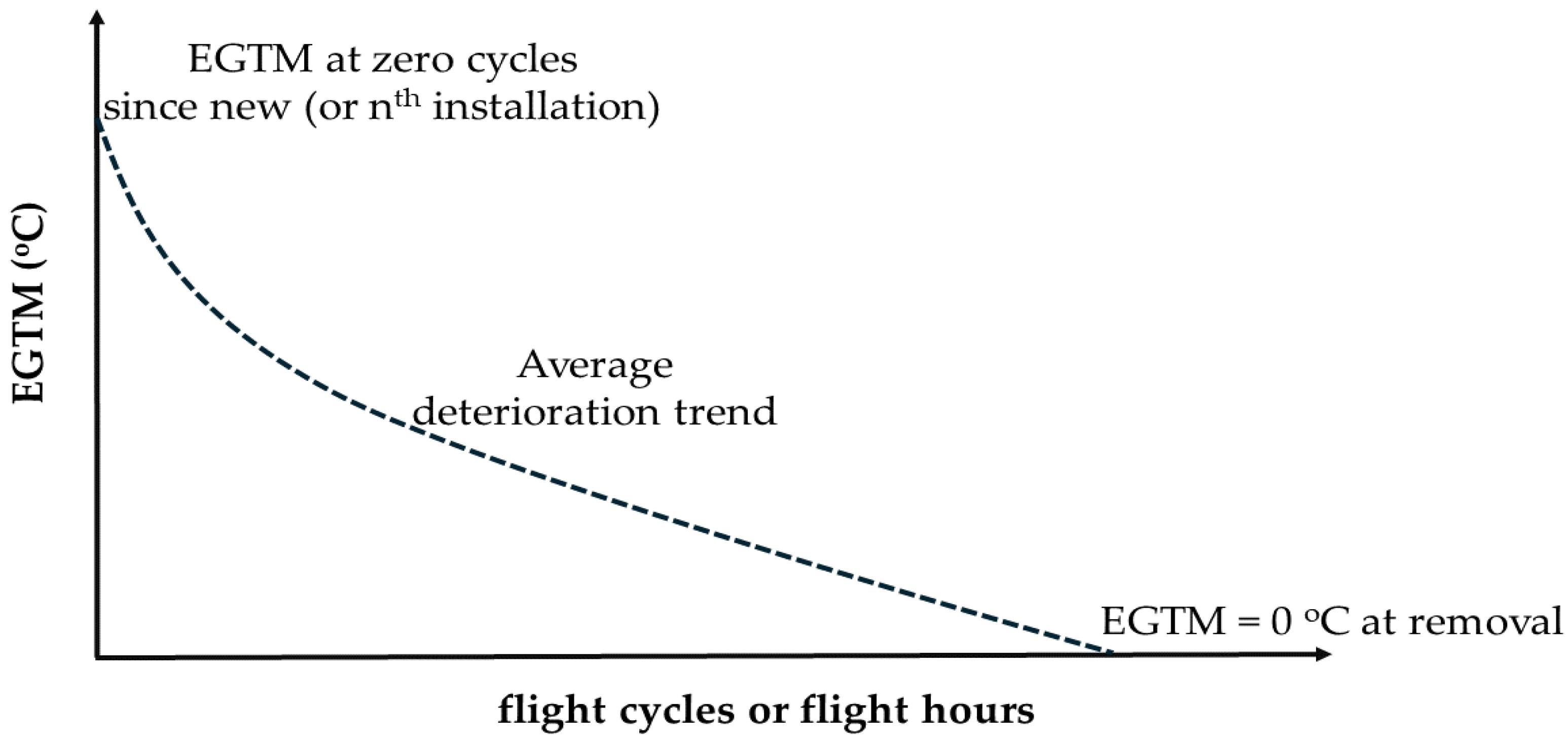
Every engine presents a representative $EGTM$ when new (or zero deterioration), a positive quantity that gradually erodes as the engine operates in service towards zero value (as depicted in Figure 1). The $EGTM$ is computed for each flight cycle (FC) throughout what is called the engine installation. An installation is referred to as the number of flight hours (FHs) or FCs in which a given engine operates in service before being sent to a shop visit (SV) for repairs. A repair might be required to regain the $EGTM$, to comply with life-limited parts (LLPs) schedules, or both. LLPs are rotors and major static structural parts that could cause a hazardous effect in the engine if they fail [22].

The initial value of the $EGTM$ (i.e., at zero cycles since the last installation) is highly dependent upon the thrust rating and the certified redline. The thrust rating, or nameplate thrust ($F_{n,NP}$), is the minimum thrust that a given engine line (i.e., group of engines of the same type) is expected to demonstrate under certain conditions agreed upon between the OEM and the airframer [23]. Typically, low thrust ratings present high $EGTMs$, and conversely, high thrust ratings present low margins.

In practice, an OEM designs an engine line to have a sufficient $EGTM$ for the highest certified rating; therefore, lower thrust ratings present an even higher $EGTM$. For example, the CFM56-3 engine family presents average $EGTM$ initialization values (i.e., at zero cycles since new) of 115, 90, and 40 °C for thrust ratings of 18,500, 20,000, and 22,000 lb_f (82,292, 88,964, and 97,861 N), respectively [24]. For the -8C family, the -8C5B1 rating ($F_{n,NP}$ = 12,670 lb_f/56,359 N), the subject of this study, is expected to have a higher $EGTM$ than the -8C5 rating ($F_{n,NP}$ = 13,360 lb_f/59,428 N), given that their $ITT$ redlines for normal take-off barely differ (948 vs. 947 °C) [21]. Unfortunately, no reliable information was found about the average $EGTM$ initialization values for these ratings; however, they will be estimated and presented in Section 5.

2.1. Engine Life in Service

This section provides the reader with a high-level understanding of the different stages of aircraft engine life during revenue service operation.

A new production engine is initially tested at the OEM’s facilities, where it must demonstrate that it complies with the performance guaranties established between the OEM and the airframer and it is fit for flying [25]. During the OEM’s acceptance outbound test, thrust ($F_n$), $SFC$, and $EGT$ (or $ITT$) measurements are taken and records are kept for historical trending purposes. Next, the engine is typically sent to the airframer to be installed in a new aircraft; however, there are times when it is dispatched directly to an airliner to serve as a spare engine. If the engine is sent to the airframer, after its installation, the airframer will perform different tests in the aircraft/engine (called production flights) before delivering the aircraft to the airliner [18]. If an engine is sent to the airline directly, it will be induced in service without the typical airframer production tests [18]. Whether an engine is dispatched to the airframer or to an airline plays a crucial role in its initial deterioration, as discussed in Section 3.2.

When an engine is installed on-wing, measurements are typically taken and recorded during take-off and cruise for altitude, Mach number ($MN$), ambient temperature, $EGT$, fuel flow (${\dot{m}}_{fuel}$), and the rotational speeds for the high- and low-pressure spools$, NH$ and $NL$, respectively. These recordings are then processed (or reduced) off-line to compute the $EGTM$ (at take-off) and the $\mathsf{\Delta }EGT$ and $\mathsf{\Delta }{\dot{m}}_{fuel}$ (at cruise). Both $\mathsf{\Delta }EGT$ and $\mathsf{\Delta }{\dot{m}}_{fuel}$ are differences (or deltas) relative to a baseline level and are used for engineering analysis and diagnostic purposes.

Once an aircraft has been delivered to the airline, an engine will begin accumulating revenue service hours (or cycles) until it gets removed for a shop visit (SV) repair/inspection. During a SV, the engine is repaired based on its ‘on-condition’ status [18], targeting only those parts/modules that need repairing, while all the others are left as received. For example, an engine work scope (i.e., the specific repair plan) may only consider HPT repair to recover performance (e.g., to regain $EGTM$) and leave all other modules, e.g., fan, HPC, low-pressure turbine (LPT), as is. While the on-condition approach is not ideal for energy efficiency purposes (non-repaired modules operate at a lower efficiency than their repaired or new level), it is worthwhile for other economical and operation purposes (i.e., less expensive engine work scopes and faster turnaround times).

It is likely that engine modules (i.e., compressors, turbines, etc.) may be interchanged among other engines being repaired during their SV time. After repairing, the engine modules are assembled, often with modules interchanged from other engines, and returned to service (in the same or another aircraft serial), which is considered a new installation. The engine will operate in service until its next SV.

Commercial aircraft engines are also classified by the number of installations they have incurred, which provides information on how many SVs an engine has had. For example, the first installation indicates an engine’s first installation when it was newly made, the second installation is its installation after its first SV, and so forth. This cycle of in-service operation and repair is repeated until the engine is retired from service, which is expected to correspond to the end of service of an aircraft (≈25 years [26]).

According to Wulf et al. [18], during its in-service operation, an aircraft engine experiences two types of deterioration, short and long term, as depicted in Figure 2. Short-term (ST) deterioration occurs during the first production flights performed by the airframer. This type of deterioration is characterized by causing a significant performance debit (e.g., an increase in $SFC$ and a decrease in $EGTM$) during a relatively short period of time, as depicted by the steep slope in Figure 2. On the other hand, long-term (LT) deterioration occurs during regular revenue service flights; its performance debit is gradual over time. Turbomachinery degradation is caused by the normal wear of its internal components (blades, vanes, seals, and clearances) and thus does not include sudden deterioration effects such as those caused by foreign objects, the so-called FOD (foreign object damage).

The LT deterioration is divided into recoverable and non-recoverable types. The former is associated with dirt and dust accumulation (in the airfoils and flow passages) that causes the degradation of both efficiency and pumping capacity and is most often seen in the compression system, i.e., fan, low-pressure compressor (LPC), and HPC. This deterioration, as its name suggests, can be recovered by a proper, regular cleaning process [27], referred to as water washing (WW). For non-recoverable LT deterioration, the performance debit is permanent and can only be partially recovered by shop visit repairs.

3. Deterioration Model

The thermodynamic deterioration model developed in this work encompasses both ST and LT deterioration; however, due to the scope of this research, only the LT deterioration for the first installation is considered, i.e., from an engine’s production to its first SV. One of the key assumptions in this study is that the $SFC$ deterioration corresponding to each turbomachinery component is equivalent between the CF6-6D and the CF34-8C5B1. This assumption was deemed reasonable considering that both engine lines were designed and produced by the same OEM, i.e., General Electric. However, assuming two (or more) engine models present the equivalent deterioration depends on several factors in addition to the technology (i.e., aerodynamics, materials, cooling), as presumed in this work. These additional factors include the engine location (under the wing or fuselage), how the engines are operated (full rated vs. derated power), and flight routes (environment: humid, polluted, or sandy).

Given that efficiency loss due to deterioration is a dynamic phenomenon, a suitable measure of time must be defined to characterize such an efficiency loss. The common industry practice for tracking the lifespan of aircraft/engines (and their parts) is by using either flight cycles (FCs) and/or flight hours (FHs). An FC encompasses all the segments of a flight (i.e., start, idle, taxi, take-off, climb, cruise, approach, landing, thrust reverse, and shutdown) [22]; the FH is the time in hours incurred during an FC.

Depending on the application (regional, short, or long haul), the FH/FC ratio can vary significantly. For example, in the case of the CRJ-700, an average FC is just over 1.6 h [28]. For a long-haul aircraft, on average, an FC lasts about 9 h [29]. Moreover, the FCs incurred between SVs are different for each engine line; therefore, a normalized parameter was established to avoid dealing with either FHs or FCs directly. This parameter was called the deterioration time index ($\tau$), which ranged from 0.0 (new engine) to 1.0 (fully deteriorated engine). The term fully deteriorated engine used in this paper refers to an engine that presents a zero $EGTM$ for high thrust ratings.

The deterioration level is assessed based on the $EGTM$ in Equation (2), in which ${EGT}_{redline}$ is the redline limit and ${EGT}_{HD,peak}$ is the $EGT$ corrected to a hot day, i.e., at full rated take-off and nominal installations (e.g., bleed settings). Notice that in Equation (2), $EGT$ can be replaced by $ITT$ without a loss in its intended meaning.

$$EGTM={EGT}_{redline}-{EGT}_{HD,peak}$$

(2)

The ${EGT}_{HD,peak}$ is obtained in a two-step process. First, the $EGT$ at full rated take-off thrust is obtained (${EGT}_{FR}$). The full rated take-off thrust ($F_n$) is computed as given in Equation (3), in which $F_{n,NP}$ is the minimum thrust value expected for any engine (i.e., −2σ) [23]. According to [30], the shortfall in thrust relative to an average engine is between 1 and 3%, depending upon the build and engine complexity. In this work, an intermediate value of 2% was considered and was embedded in Equation (3). Second, the ${EGT}_{HD,peak}$ is calculated as per Equation (4), in which ${\theta }_{HD}^x=\frac{T_{0,HD}}{T_{std}}$; the $T_{0,HD}$ corresponds to the total temperature of the engine’s incoming air projected for a hot day, $T_{std}$ is the standard-day temperature at sea level, 518.67 R (288.15 K), and x is the suitable exponent (x = 1.0 in this study).

$$F_n=1.02 \times F_{n,NP}$$

(3)

$${EGT}_{HD,peak}={EGT}_{FR}\times {\theta }_{HD}^x$$

(4)

The thermodynamic deterioration model helps to translate the projected loss in component efficiency ($∆\eta$) into a decrease in the $EGTM$ and an increase in fuel consumption ($\delta f_c$) through physics-based relationships (i.e., mass and energy balances).

The authors of this work believe that the only way to accurately account for engine component efficiency loss ($∆\eta$) is through empirical studies, such as those presented in [18,19]. These studies are the most comprehensive work found in the literature on real aeroengine deterioration assessments representative of an engine line. Similar studies for more recent engine lines are not easy to replicate as the costs and effort associated with such studies are likely prohibitively high. More importantly, empirical studies aim to reflect the deterioration of an engine model fleet, which, by definition, represents an average deterioration trend. Deterioration trends for single or small groups of engines might not agree with the average trend; thus, they are not recommended for predictions concerning the average behavior of an engine fleet.

3.1. Thermodynamic Baseline Model

A thermodynamic engine cycle model was developed by Gurrola Arrieta and Botez [20] to approximate the performance of the CF34-8C5B1. This cycle model, called the CM-8C5B1, was obtained by matching an off-design cycle model to the data obtained from a Level-D high-fidelity flight simulator representing the CRJ-700, the so-called Virtual Research Simulator (VRESIM). More details about the VRESIM are presented in Section 4.

An initial model was established using the Aerothermodynamic Generic Cycle Model (AGCM) and the aerothermodynamic design point presented in [31]. Next, this initial model was recalibrated to represent the CF34-8C5B1 engine with data obtained from the VRESIM. The recalibration consisted of finding the values of independent variables in the cycle model such that the differences in thrust and fuel flow between the VRESIM and the cycle model were minimized. The accuracy of the CM-8C5B1 was within ±5.0% for the power settings of interest.

3.2. Thermodynamic Deterioration Model

This model was established based on adiabatic efficiency losses ($∆\eta$) for the turbomachinery components, fan, HPC, HPT, and LPT, derived in [18]. It is worth noting that the CF34-8C5B1 engine does not account for an LPC (or booster); thus, an LPC is not considered in the model.

The average engine deterioration of the CF34-8C5B1 was considered equivalent to that observed for the CF6-6D [18]; based on this premise, ${{∆SFC}_{CF34-8C5B1}\equiv ∆SFC}_{CF6-6D}$. The total $\mathsf{\Delta }SFC$ can be interpreted as the linear combination of the individual (i) turbomachinery component contributions, as expressed in Equation (5).

$${\mathsf{\Delta }SFC}_{total}=\sum _i\mathsf{\Delta }{SFC}_i$$

(5)

By knowing the $\mathsf{\Delta }{SFC}_i$, the corresponding ${∆\eta }_i$ can be computed based on the set of derivatives presented in

Table 1. $SFC-$ efficiency ($\frac{\partial SFC}{\partial {\eta }_i}$) partial derivatives at cruise (per $\mathsf{\Delta }{\eta }_i$ = −1.0%).

Component (i)	CF34-8C5B1 (%)	CF6-6D (%) [18]
Fan	+0.50	+0.54
HPC	+0.51	+0.56
HPT	+0.71	+0.78
LPT	+0.66	+0.55

. These derivatives were obtained by running the CM-8C5B1 at 35,000 ft (10,668 m), $MN$ = 0.80, $\mathsf{\Delta }T$ = 0.0, and $F_n$ = $F_{n,CR}$. The $F_{n,CR}$ value corresponds to the estimated cruise thrust. The same derivatives for the CF6-6D are presented in Table 1 for reference.

The salient ST and LT deterioration results presented by Wulf et al. [18] are briefly discussed next. These results are the outcome of a thorough engineering assessment performed utilizing data from different types of observations, such as on-wing cruise data (from production or in-service flights), test cell (TC) outbound and inbound data, and visual inspections and measurements of the engine parts.

3.2.1. Short-Term Deterioration

The short-term (ST) deterioration is due to maneuvers that are not typical of revenue service flights and which are performed during airframer production tests [18]. The so-called hot rotor reburst (HRR) is the likely cause of this deterioration. During HRR, an engine is brought from high to low power (and vice versa) quite rapidly, causing the HPT case and the rotor blades to rub due to differences in growth expansion. The rubs that occur during HRR produce a significant loss in HPT efficiency and some minor losses in the HPC and LPT.

One interesting finding presented in [18] is that only those engines that went through airframer production flights showed this ST deterioration, whereas those sent directly to the airliner (spare engines) did not. The justification for this difference is attributed to the fact that the engines shipped directly to the airliner do not incur any atypical revenue service maneuvers (such as the HRR).

The contributions to $SFC$ that increase due to ST deterioration are presented in

Table 2. Short-term loss summary.

Component	$\Delta \mathit{S}\mathit{F}\mathit{C}$ at Cruise (%) [18]	$\Delta \mathit{\eta }$ (CF6-6D, %) [18]	$\Delta \mathit{\eta }$ (CF34-8C5B1, %)
HPC	+0.03	−0.05	−0.05
HPT	+0.74	−0.95	−1.04
LPT	+0.04	−0.07	−0.06
Total	+0.81	--	--

. The total $SFC$ loss is significant ($∆SFC$ = +0.81%) and must be tallied separately, given that it happens in a short period of time. According to Ethell [32], 0.1% in $SFC$ is considered as a significant figure by airlines.

It should be noted that the ST deterioration split shown in Table 2 came from the hardware inspection analysis presented in [18]; the actual measured cruise $SFC$ increase was +0.9%. Wulf et al. [18] concluded that both these values are within precision requirements. Table 2 also presents the associated turbomachinery efficiency losses ($∆\eta$) for the CF6-6D (for reference) and for the CF34-8C5B1, both computed using the derivatives presented in Table 1.

3.2.2. Long-Term Deterioration

The data analysis performed by Wulf et al. [18] included both first and subsequent installations. However, for the scope of this paper, only the salient results obtained from the first installation are presented. The in-service data analysis consisted of a sample of engines in their first installation period, all of which had gone through the airframer production flights, i.e., had already experienced ST losses.

The information from both in-service cruise and TC data allowed Wulf et al. [18] to establish the measured LT deterioration when an average engine was removed for its first SV, which equated to $∆{SFC}_{LT}$ = +1.70%. To compute the total $SFC$ increase (relative to the outbound new engine test), the ST loss ($∆{SFC}_{ST}$ = +0.81%) must be added; thus, $∆SFC=$ +2.51%. The conclusion from these results is that, on average, an engine increases its fuel burn (or $∆SFC$) at cruise by +2.51% (relative to its new state condition) when it is sent to its first SV; such an increase is due to the typical airframer production flights (+0.81%) and the engine’s normal revenue service life experience (+1.70%).

Moreover, Wulf et al. [18] presented the results of an engineering assessment performed by a group of experts (from General Electric) over each module. They correlated the inspection results with the increase in $SFC$ with the goal of estimating the shape of the deterioration factors (i.e., clearance increase, airfoil surface quality, etc.) over time. Wulf et al. [18] claimed that these curves are not necessarily reliable due to the limited data and the large reliance on engineering judgment but that they do present a reasonable estimate. Despite these caveats, the authors of the present paper deemed these deterioration curves as one of the best references available in the literature.

The observations/conclusions about hardware deterioration mentioned above were also helpful in this research to define which losses should not be considered. For example, losses caused by a particular repairing procedure in the CF6-6D and those associated with modules that do not occur in the CF34-8C5B1 (e.g., the LPC of a booster) can be ignored.

To relate the efficiency loss curves from the CF6-6D to those of the CF34-8C5B1, a normalized parameter called the deterioration time index ($\tau$) was introduced as the total FHs during the first installation phase were not the same for these engine models. For the CF6-6D, the average SV occurs after about 4000 FHs [18], whereas for the CF34-8C5B1, this is expected to happen at about 21,000 FHs (the details about this figure are presented in Section 5). The $\tau$ parameter assumes a linear relationship with the total FHs of both the CF6-6D and the CF34-8C5B1. For such linear relationships, the following boundary conditions must be met: for FH = 0.0, $\tau$ = 0.0, and for FH = ${FH}_{@SV}$, $\tau$ = 1.0. The ${FH}_{@SV}$ is the average FHs at which an SV takes place (e.g., 4000 h for the CF6-6D and 21,000 h for the CF34-8C5B1).

The LT efficiency deterioration for each turbomachinery component presented in [18] is shown in Figure 3 as a function of $\tau$. The numbers presented in this figure should be understood as deviations from the ST efficiency loss curve and interpreted as efficiency losses, i.e., −1 × $\mathsf{\Delta }{\eta }_i$.

The data for ST and LT efficiency losses presented in Table 2 and Figure 3, respectively, provide key insights about the expected levels for component efficiency loss throughout an engine life. It is worth noting that the efficiency loss (ST and LT combined) does not exceed 1.4% for any component. One of the biggest challenges faced by researchers is to define realistic levels of efficiency losses. Some of the models discussed in Section 1 considered greater efficiency losses than those presented by [18]. Moreover, some of them ignored the deterioration presented in the low-pressure system (fan and LPT).

4. Aircraft Fuel Consumption

To evaluate the fuel consumption ($f_c$), three representative types of missions were simulated: short (0.4 h), average (1.4 h), and long (2.5 h). These missions were defined by analyzing the FHs of a sample of two-hundred and thirty-five (235) CRJ-700 flights across North America extracted from an open-source database (flightaware.com, accessed on 6 June 2023), which are presented in Figure 4. These flights were performed between 2 June 2023 and 5 June 2023 and included different tail numbers and different operators. There was nothing particular about these dates other than their information was available when the database was queried for the purpose of this research.

For the short-mission flight, the time was representative of the shortest duration flights from Figure 4 (15 flights were between 25 and 35 min). The average duration of the flights from this sampling is 1.3 h; however, the average missions considered in this paper lasted 1.4 h. The latter number is close enough to that reported in [28] (i.e., 1.6 h). Finally, the long-mission flights correspond to a +2σ flight (i.e., 2.5 h).

Three specific flights depicted in Figure 4 (indicated as colored triangles) were used as references to define the short, average, and long missions used in this research. Data such as stage distance ($d$), cruise altitude, and Mach Number ($MN$) were used to define the corresponding missions in this paper. The climb and descent schedule objectives for these research missions are presented in

Table 3. Climb and descent schedules.

	Altitude ft [m]	$\mathbf{IAS}/\mathit{M}\mathit{N}$/RD IAS: Indicated Airspeed, Knots [km/h] RD: Rate of Descent, ft/s [m/s]
Climb	5000/24,000/CR altitude [1524/7315/CR altitude]	$160/290/\mathrm{Cruise} MN$ $[296.3/537/\mathrm{Cruise} MN$]
Descent	CR altitude/5000 [1524]	RD = 1200/IAS = 160 [RD = 365.8/IAS = 296.3]

. The short and long missions present deviations from this schedule. In the short mission, the cruise is performed at 12,000 ft (3658 m), and its cruise $MN$ was maintained at about 0.55. In the long mission, the aircraft descends to about 32,000 ft (9754 m) and performs a brief cruise hold (about 5 min) before concluding its final descent. The high-level characteristics of these missions and the detailed times per flight mission are presented in

Table 4. Research missions’ high-level characteristics.

Mission	Distance, NM (km)	$∆\mathit{t}$, min (h)	Cruise Altitude, ft (m)	$\mathbf{Cruise} \mathit{M}\mathit{N}$, None
Short	111 (205.5)	25.10 (0.4)	12,000 (3658)	0.55
Average	539.4 (998.9)	83.17 (1.4)	34,000 (10,363)	0.75
Long	999.1 (1850.3)	149.40 (2.5)	36,000 (10,973)	0.75

and

Table 5. Missions’ phases break-up times.

Short
	Δt (min)	Δt (% relative trip time)
Take-off	0.65	2.6
Climb	4.57	18.2
Cruise	8.58	34.2
Descent/approach	11.30	45.0
Total	25.10	100.0
Average
Take-off	0.83	1.00
Climb	16.45	19.8
Cruise	38.90	46.8
Descent/approach	26.99	32.4
Total	83.17	100.0
Long
Take-off	0.78	0.5
Climb	17.75	11.9
Cruise1	88.47	59.2
Descent1	5.20	3.5
Cruise2	4.80	3.2
Descent2/approach	32.40	21.7
Total	149.40	100.0

, respectively.

To obtain the best predictions of the actual aircraft $f_c$ in these three types of missions, a Level-D flight simulator was used. Level-D flight simulators encompass real-time models to simulate both the aircraft and the engine and have played a pivotal role in the research of the Laboratory of Applied Research in Active Control, Avionics, and AeroServoElasticity (LARCASE). Aircraft and engine models for the Cessna Citation X and the CRJ-700 have been developed at the LARCASE [33]. Examples of their work on engine models include system identification [34,35,36], adaptive algorithms [37], and neural networks [38,39,40]. Different cycle model analyses have also been performed at the LARCASE over the past few years [31,41,42,43].

The Virtual Research Flight Simulator (VRESIM), designed and manufactured by CAE Inc., was utilized for this research (Figure 5). The VRESIM represents the CRJ-700 aircraft. The three research flight missions (short, average, and long) were first simulated in the VRESIM. The aircraft and engine models embedded in the VRESIM interact with each other to determine the appropriate power setting (i.e., ${NL}_{corr}$) for specified flight conditions and environmental control system (ECS) bleed demands. The ECS oversees aircraft cabin ventilation and is supplied by air extracted from both engines. The engine model in the VRESIM encompasses an accurate representation of the full authority digital engine control (FADEC), which manages the engine power setting during in-service operation.

The data obtained from the VRESIM were then input to the CM-8C5B1. The flight conditions (altitude, $MN$, and ambient temperature deviation), power settings (${NL}_{corr}$) and bleed settings for each data point in the missions were provided to the cycle model. The VRESIM and the CM-8C5B1 (for $\tau$ = 0.0) simulations correspond to a new engine condition (or zero deterioration). The $f_c$ during each flight phase and the so-called trip fuel (defined in Section 4.1) were compared between the VRESIM and the CM-8C5B1 to validate the results from the latter.

The average mission was then simulated on the CM-8C5B1 to account for other levels of deterioration, with $\tau$ = 0.025, 0.050, 0.10, 0.25, 0.50, 0.75, and 1.00. A similar set of $f_c$ comparisons was generated for each level of deterioration using cycle model results with zero deterioration ($\tau$ = 0.0) as a reference.

4.1. Mission Assumptions

The mission assumptions for the VRESIM are presented next, followed by those pertaining to the cycle model.

The aircraft accounted for two engines being operative with nominal ECS bleed extraction from both. No wing or nacelle bleed anti-icing was assumed. Additionally, the conditions considered were standard day temperature and no wind effects (i.e., no additional aircraft drag).

In this study, the operating empty weight (OEW), payload, and fuel weight (FW), as percentages of the take-off weight (TOW), were 66.4, 17.6, and 16.0%, respectively. The payload assumes a passenger load factor ($L_f$) of 78% (the ratio of the number of passengers to the available seats). The $L_f$ was obtained from statistics provided by the Bureau of Transportation Statistics (https://www.transtats.bts.gov/, accessed on 21 January 2024) and based on one of the major CRJ-700 operators in North America. Moreover, $L_f$ represents the average computed value between 2002–2019 and the years 2022 and 2023.

Take-off and landing took place at sea-level altitude. The flights accounted for take-off roll, climb, cruising, and descent up to touch down performed over the same x-y plane, i.e., no turning. Taxi-out, reverse, and taxi-in fuel use were not considered. Thus, both the block time and the fuel consumption were computed based on the so-called ‘trip fuel’ [44], which encompassed the flight phases considered in this work.

The take-off roll is performed at full rated power (i.e., no reduced or flex thrust). The VRESIM data acquisition scan rate was set to 1 Hz, i.e., each data point within the mission flights was sampled every second.

The assumptions concerning the cycle model are presented now. A group of parameters obtained from the VRESIM’s output data were input to the cycle model. These data include the altitude, Mach number ($MN$), ambient temperature deviation from standard atmosphere ($\mathsf{\Delta }T$), ECS bleed setting (flow and pressure), and corrected fan speed (${NL}_{corr}$). A validation of the input boundary conditions to the cycle model is presented in Figure 6 for the average-time mission. This validation ensured that the cycle model ran under the same conditions as the VRESIM real time model, thus avoiding the introduction of a potential input bias [43].

The thermodynamic model accounts for the thermodynamic properties of a kerosene-based conventional aviation fuel with a hydrocarbon ratio of 2:1 and a lower heating value of 18,500 Btu/lb_m (43,031 kJ/kg). Moreover, the engine’s incoming air was considered dry (i.e., no humidity).

It was assumed that both left and right engines were in their first installations and that both went through typical airframer production flights, i.e., incurred initial ST losses. Both engines present a dirty fan throughout their first installation. This assumption defines the expected level of deterioration based on the curves presented in Figure 3, which is believed to be the most conservative scenario. Engine WWs occur at the operator’s discretion; henceforth, the selected assumption means that no WWs are performed, i.e., a harsher fan deterioration impact is expected.

During each mission, the ${NL}_{corr}$ remained unchanged throughout the deterioration levels as it was assumed the FADEC did not adapt the power setting to account for deterioration.

For each level of deterioration, the $ITTM$ and the fuel consumption ($f_c$) are computed. The $ITTM$ is computed by Equation (2), in which the ${ITT}_{redline}$ = 947 °C and ${ITT}_{HD, peak}$ is experienced during the take-off roll under a hot-day temperature condition (ISA + 27° F/+15 °C). The $f_c$ is based on a cumulative summation of the product of the fuel flow rate (${\dot{m}}_{fuel}$) and the $∆t$, as expressed in Equation (6).

$$f_c=\sum _i^n{\left({\dot{m}}_{fuel}∆t\right)}_i$$

(6)

The trip fuel intensity ($\mathsf{\Gamma }$), depicted in Equation (7), is analyzed to understand the aircraft/engine efficiency. This metric represents how much fuel (gallons or litters) is spent to move each passenger one unit of distance (NM or km). In Equation (7), $f_{c,trip}$ is the fuel consumption for the trip, $PL$ is the product of the passenger load factor ($L_f$) and the aircraft’s available seats, and $d$ is the stage distance.

$$\mathsf{\Gamma }=\frac{f_{c,trip}}{PL\times d}$$

(7)

Finally, the results discussed in the next section must be understood as average values, meaning that they are representative of an average-quality engine. This claim is supported by the fact that the thermodynamic cycle model represents an average engine. Moreover, the efficiency losses derived in [18], used in this work to define the thermodynamic deterioration model, correspond to the conditions of an average of the engines in a fleet.

5. Results Discussion

The results are presented in two parts, first, those for an engine with zero deterioration (i.e., a new engine). The predictions of the CM-8C5B1 are compared with data obtained from the VRESIM for validation and then are used to derive insights about the fuel consumption ($f_c$) during each mission. The second part of our discussion is dedicated to the deteriorated engine. The discussion is focused on the $ITTM$ and $f_c$ for the average mission only. The justification behind this approach is presented next.

For short-range applications (such as the CRJ-700), low cycle fatigue (LCF) becomes a limiting factor in the engine life [16]. LCF refers to the number of flight cycles (FCs) under high stresses, presented typically during full rated take-offs, having an impact on component material properties. According to Donaldson et al. [45], engine life will only be affected by take-off thrust for an LCF-related mode failure. Based on these claims, similar conclusions can be drawn concerning engine deterioration for the three research missions (short, average, and long), given that they present similar take-off characteristics (i.e., flight conditions, power setting, and bleed setting).

The comparison for thrust and fuel flow between the VRESIM and the CM-8C5B1 for an average mission is presented in Figure 7a. This figure shows that the errors for both thrust ($F_n$) and fuel flow (${\dot{m}}_{fuel}$) are overall within ±5.0% during take-off, climb, and cruise. These observations agree with the results presented by Gurrola Arrieta and Botez [20]. Higher errors (outside ±5.0%) are present during descent, mainly at low power settings (i.e., flight idle). These errors are accentuated by the noise in the bleed setting during descent, as observed in Figure 6c; however, they do not seem to contribute significantly to driving high differences in the cumulative $f_c$, as shown in Figure 7b, i.e., the VRESIM and the CM-8C5B1 curves closely follow each other.

The $ITT$ was also a parameter of interest during our results analysis, so it was necessary to present the accuracy of the CM-8C5B1 vs. that of the VRESIM. Unfortunately, due to an omission in the script used to store data during the mission simulations, the $ITT$ was inadvertently excluded during the VRESIM simulations and thus is not shown in Figure 7a. Nonetheless, the data gathered in a previous work by the authors in [20] was used to generate a set of comparisons that provided a good indication of the CM-8C5B1 $ITT$ accuracy in the region of interest, as depicted in Figure 8. The region of interest encompasses the take-off phase where the aircraft is taken from static ($MN=$ 0.0) to dynamic conditions (up to $MN$ ≈ 0.25) at full rated power. The $ITT$ errors at $MN$s of 0.0, 0.151, and 0.302 considering the CF34-8C5B1 rated power are +9, −12, and −6.6 °C, respectively.

The $f_c$ computed for each flight phase and the trip fuel amounts seem to show good agreement between the VRESIM and the CM-8C5B1 (see Figure 9); the errors are overall less than ±2.0%. However, for the short mission, the errors for cruise, descent, and total (trip fuel) are outside these error bands. These increased errors are driven by the ${NL}_{corr}$ setting during cruise and descent. According to [20], the accuracy of the CM-8C5B1 declines below ${NL}_{corr}$ = 85% (which is the case for the short mission), tending to underpredict the fuel flow rate. The errors observed in the total trip fuel consumption are −3.6, +0.9, and +0.6% for the short, average, and long missions, respectively. These small errors provide confidence in the predictions generated by the cycle model and are deemed acceptable for further analyses.

The $f_c$ is a function of altitude, $∆t$, and engine power setting. However, to circumvent having to analyze such a complex relationship, an approximation can be generated by computing the ratio of $∆f_c$/$∆t$, in which $∆f_c$ and $∆t$ represent the fuel consumption and the time spent during each flight phase, respectively, as a percentage relative to their total trip values (see

Table 6. Fuel consumption for time ratios, $∆f_c$/$∆t$.

Flight Phase	Short	Average	Long
Take-off	2.7	3.2	3.4
Climb	1.9	1.8	1.9
Cruise	0.9	0.9	0.9
Descent/approach	0.6	0.6	0.8

).

To reduce fuel consumption, it is desirable to have short $∆t$ for those flight segments in which $∆f_c$/$∆t$ values are high, like take-off or climb. Figure 10 presents the $∆t$ and $∆f_c$ splits during each flight phase relative to their total. The take-off phase takes the least time in all three mission types ($∆t$ ≤ 2.6%), which is as expected based on its high $∆f_c$/$∆t$; therefore, the net effect is a small $∆f_c$. In the case of climb, $∆t$ ≤ 20% in all three mission types. The climb $∆f_c$ for the short mission shows the highest amount, whereas for the average and long missions, the climb $∆f_c$ is less than that of the cruise. Even though the time spent in climb is less than one fifth of the total mission time, its $∆f_c$/$∆t$ is the second highest; thus, there is a considerable $∆f_c$ penalty.

For the missions analyzed in this paper, the time during cruise does not overshadow the time spent in other segments. For example, for a short mission, the $∆t$ during descent ($∆t$ = 45.0%) is greater than that of cruise ($∆t$ = 34.2%), which translates to the two flight phases having a close $∆f_c$ between them ($∆f_c$ = 26.0% during descent, whereas for cruise, $∆f_c$ = 30.6%).

The next comparison is based on the fuel consumption relative to the available fuel at take-off, which was the same for all three missions (i.e., 16% of the TOW). After completing the short, average, and long missions, the fractions of fuel remaining in the tank were 0.83, 0.54, and 0.24, respectively (see

Table 7. Fuel available after landing (as a fraction of the fuel weight at take-off).

Mission	Fraction
Short	0.83
Average	0.54
Long	0.24

). These figures can be significantly affected by other fuel quantities not considered in this research (e.g., taxi-in/-out, contingency fuel, etc.). For example, according to the results presented in [46], the $f_c$ during taxi-in and -out is about 8.5% of that of the total mission.

The last comparison is performed to evaluate the fuel trip intensity ($\mathsf{\Gamma }$), presented in

Table 8. CRJ-700 trip fuel intensity (for new engines).

Mission	$\Gamma$ US Gallon (Litter)/NM (km)/Passenger	$\Gamma \times \mathit{d}$ US Gallon (Litter)/Passenger
Short	0.039 (0.080)	4.35 (16.47)
Average	0.023 (0.047)	12.45 (47.14)
Long	0.021 (0.042)	20.56 (77.81)

. Here, it is clear the aircraft becomes significantly more efficient when flying an average mission rather than a short one. The efficiency goes from 0.039 to 0.023 US gallons/NM/passenger (or 0.080 to 0.047 litters/km/passenger), which represents an $f_c$ improvement of 41%. Another 6% improvement can be achieved when flying a long mission. These comparisons are by no means comprehensive due to their limiting assumptions (TOW and flight profiles); however, they help to generate confidence based on the results from other studies. For example, in [28], for a 513 NM (950.1 km) CRJ-700 mission, the $\mathsf{\Gamma }$ was 0.022 vs. 0.023 reported in this work for the average mission with $d$ = 539.4 NM (998.9 km). The numbers presented in Table 8 could be used to generate fuel estimates of costs and emissions; however, such estimates are outside of the scope of the current research.

Next, the focus is on the deteriorated engine results. The predicted $ITTM$ for a new engine (i.e., zero deterioration) is 55.2 °C, as shown in Figure 11. The ${ITT}_{HD,peak}$ occurs at $∆t$ = 17 s after the initiation of the take-off roll, at which the $MN$ = 0.181. The $ITTM$ presents considerable erosion ($∆ITTM$ = −14.3 °C) from $\tau$ = 0.0 to 0.025, mostly driven by the ST losses. From $\tau$ = 0.1 to 1.0, there is an almost linear loss of about $∆ITTM$ = −1.2 °C per $\mathsf{\Delta }\tau$ = 0.1 (or 10% deterioration). More importantly, our predictions suggest that the $ITTM$ for a fully deteriorated engine ($\tau$ = 1.0) is 26.4 °C. The total $ITTM$ loss (from new to fully deteriorated) is −28.8 °C, of which half occurs for $\tau$ ≤ 0.025.

The results presented above suggest that the CF34-8C5B1 rating will not present $ITTM$ constraints during its life in service. In other words, a low (or null) $ITTM$ may not be the main cause for removing an engine from operation, not even considering $ITT$ variation, given that the figures discussed here are considered to be representative of average-quality engines. According to [18], the $EGTM$ variation for the CF6-6D is about ${\sigma }_{EGTM}$= 9 °C. Assuming this variation may also be representative of the CF34-8C5B1, then even a −2σ engine would have some margin to redline at $\tau$ = 1.0, i.e., ${ITTM}_{-2\sigma }$ = 8.4 °C. In most cases, the service time of life-limited parts (LLPs) will be the main reason for sending a CF34-8C5B1 to shop visits.

For higher-rated engines, such as the CF34-8C5 ($F_{n,NP}$ = 13,360 lb_f/59,428 N), our predictions suggest that the initial $ITTM$ would be 26.8 °C and when fully deteriorated would be −2.0 °C (see Figure 11). This prediction was derived with the CM-8C5B1 based on the differences in thrust ($\mathsf{\Delta }{F}_n$ = +5.45%) and $ITT$ ($\mathsf{\Delta }ITT$ = +1 °C) between the -8C5 and -8C5B1 ratings at sea-level static, ISA temperature, and the no ECS bleed extraction condition. These results suggest that for the -8C5 rating, an average engine will present $ITTM$ problems towards the end of its life, i.e., in the region where $\tau$ lies between 0.84 and 1.0. Therefore, the -8C5 rating is more likely to be sent to a repair shop to recover its performance and thus regain the $ITTM$. It is noteworthy that the -8C5B1 and -8C5 are two different thrust ratings provided for the same engine but for different versions of the CRJ aircraft, the former intended for the CRJ-700 and the latter for the CRJ-900.

The fact that the -8C5B1 rating shows no restriction on the $ITTM$ is not unique to the CF34 engine family; other engine families such as the CFM56-3 present a similar situation in which lower ratings show a significant $EGTM$ compared to higher ratings, as discussed in Section 2. The fuel consumption increment relative to the new state level ($\delta f_c$), as with the $ITTM$, observed a significant rise during the first part of the engine life: at $\tau$ = 0.025, the $\delta FC$ = +1.0%. An almost linear relationship is observed between $\tau$ = 0.1 and 1.0 at a rate of $\delta f_c$ = 0.23% per $\mathsf{\Delta }\tau$ = 0.1.

To estimate the increase in $f_c$ throughout the engine life (from $\tau$ = 0.0 to 1.0), the area under the $\delta f_c$ curve must be approximated, i.e., ${\int }_{0.0}^{1.0}\delta f_{c}d\tau$.

Table 9. Cumulative fuel consumption increase.

$\mathit{\tau }$ (None)	${\int }_{\mathit{\tau }1}^{\mathit{\tau }2}\mathit{\delta }{\mathit{f}}_{\mathit{c}}\mathit{d}\mathit{\tau }$ (%)
0.0–0.025	0.01
0.025–0.05	0.03
0.05–0.10	0.06
0.10–0.25	0.24
0.25–0.50	0.50
0.50–0.75	0.63
0.75–1.00	0.78
Total	2.25

presents the approximated areas under the curve (computed by means of the trapezoidal rule) for each line segment. It is expected that an average CF34-8C5B1 engine shows a total cumulative $\mathsf{\delta }{f}_c$ = 2.25% throughout its operational life (from $\tau$ = 0.0 to 1.0). For a CRJ-700 operating with two engines in its first installation (from new condition to fully deteriorated) translates to $\mathsf{\delta }{f}_c$ = 4.5%.

Finally, calculations were performed to obtain an approximate idea of how much fuel (in gallons/liters) $\mathsf{\delta }{f}_c$ = 4.5% represents based on the figures discussed above. Considering that both engines fly 21,000 h before their first SV, and assuming 60% of the time the aircraft performs an average mission, while the other 40% is equally divided between short and long missions, the total number of FCs is 14,500; this latter number matches the HPT’s lower limit of LLPs presented in [28]. Moreover, assuming the load factor ($L_f$ = 78%) remains constant throughout the FCs, then the number of passengers traveled equates to about 767,000. In other words, it is predicted that more than three quarters of a million passengers are flown by a single CRJ-700 between the time the engines are new and their first SV. Scaling the values presented in Table 8 by 1.045, we obtained $\delta f_c$= 429,870 US gallons (1.627 × 10⁶ L). In other words, it is predicted that a CRJ-700 would consume about 4.3 × 10³ US gallons (1.627 × 10⁶ L) more fuel (relative to its new production state) just due to the deterioration of its engines during their first installation. These predictions correspond to an average-quality engine, and they need to be adjusted to account for other types of engines (i.e., a −2$\sigma$ quality engine) in case such figures must be scaled to understand the potential impact of any type of aircraft (e.g., single/various fleet operator, overall fleet, etc.).

6. Conclusions

The evidence suggests that gas turbine engines will continue to be used in the forthcoming decades and fuel consumption will still be a significant concern for commercial aviation, despite the introduction of sustainable aviation fuels. Therefore, reliable models that help to predict the increments in fuel consumption throughout aircraft/engine lifespans are still needed. Thermodynamic models developed for conventional fuels, like the one presented in this work, could be leveraged to be used with sustainable fuels, provided they present similar hydrocarbon ratios and heating values.

The proposed model provides a mean for assessing the effect on engine performance caused by turbomachinery component deterioration, one of the key factors affecting aircraft fuel consumption. This model accounts for the efficiency losses that are expected during in-service operation and thus is designed to provide more realistic predictions than other models developed for the same purpose. The proposed model showed good accuracy for computing trip fuel consumption assessments relative to the VRESIM’s real-time model under new engine conditions as the errors observed in the short, average, and long missions were −3.6, +0.9, and +0.6%, respectively.

The importance of assessing the $ITTM$ to determine engine deterioration was stressed in this work, an aspect that is commonly overlooked in most research in this area. The results reveal that a CF34-8C5B1 rating may not present $ITTM$ problems during its life in service, i.e., it is unlikely that an engine might reach or exceed redline limits during a take-off roll, and thus, they are only likely to be removed from in-service operation and sent to a repair shop to comply with life-limited part inspections and not to improve their performance. As a final observation, the predicted increment in fuel consumption throughout the engine life is 2.25%. The impact in fuel consumption for a single CRJ-700 with two fully deteriorated engines translates to 4.5%, which is equivalent to 429,870 US gallons (1.627 × 10⁶ L).