Design and Analysis of the Integrated Drag-Free and Attitude Control System for TianQin Mission: A Preliminary Result

Abstract

This article explores novel in-orbit drag-free technology that can be utilized for deep space detection scientific missions. In this study, we considered a two-test-mass drag-free method and analyzed the design of the drag-free and attitude control system for the TianQin mission. The entire control system was comprehensively designed, including an actuator allocation design and controllers for two test masses and one spacecraft, with a total of 18 degrees of freedom. Furthermore, stability analysis was conducted. Based on our design, numerical analysis and simulations were performed assuming geocentric orbit conditions in the TianQin mission, confirming the feasibility of this aerospace engineering concept. The versatility of the design allows for its application to scientific observations across various disciplines by modifying the structure of the simulation environment, and consequently, the approach discussed in this study holds significant practical implications for effectively accomplishing deep space observation tasks.

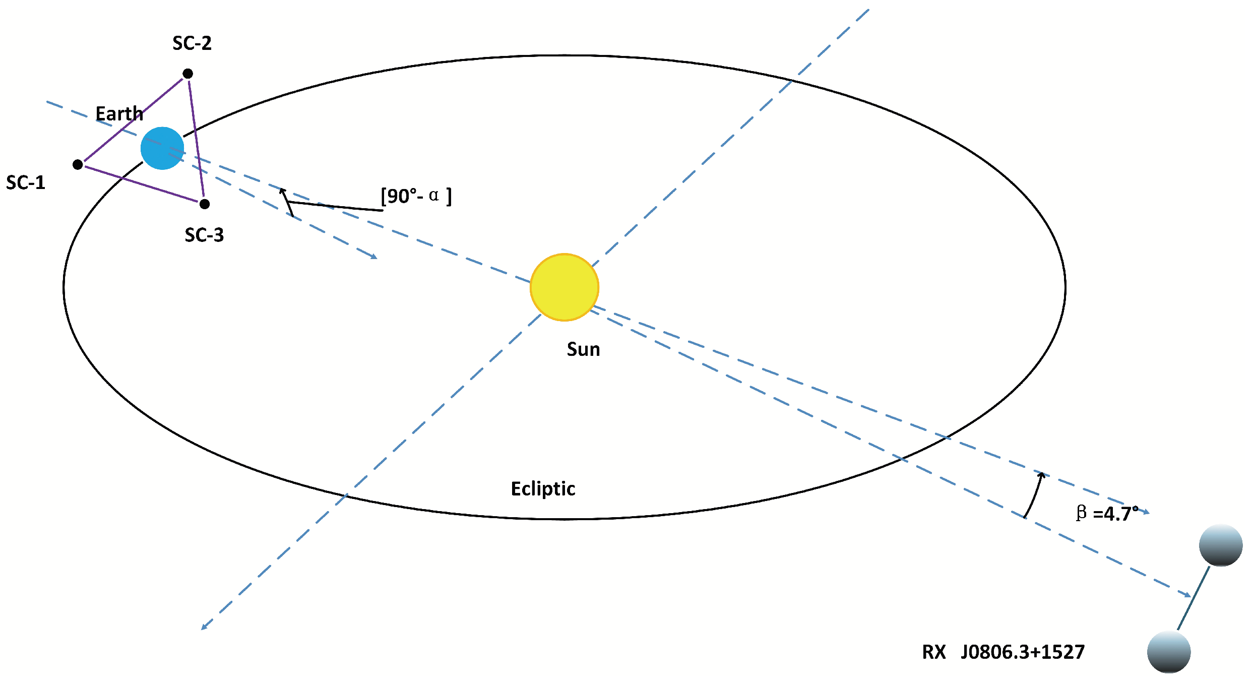
1. Introduction

The advancement of spacecraft technology has sparked a growing interest among researchers in deep space exploration, as evidenced by the increasing utilization of observation payloads on spacecraft to study distant celestial objects, and the ability to closely approach and investigate specific celestial bodies [1,2,3,4,5,6]. Consequently, drag-free control has emerged as a highly regarded technique in aerospace engineering due to its capacity for providing a stable platform in scientific spacecrafts [7], particularly for some in-orbit scientific experiments, or provide a observation platform for gravitational waves from deep space [8,9,10,11,12,13,14,15,16,17,18,19], i.e., the TianQin mission [11,12,13,14,15]. The TianQin mission, which is proposed to detect and characterize gravitational waves in the millihertz frequencies, relies on a spacecraft constellation with an orbital radius of 100 thousand km, where it consists of three spacecrafts flying with an equilateral triangular configuration in a geocentric orbit with a high-precision requirement of residual acceleration on the test masses of ${10}^{-15}$ m/s²/Hz^1/2 between 1 mHz and 1 Hz in a drag-free control design. By incorporating a drag-free design, the spacecrafts compensate for nonconservative forces through the tracking of one or more free-fall test masses, enabling them to achieve an idealized trajectory in space. The utilization of drag-free control technology dates back to the 1960s and has found widespread application in the field of space science [7,20,21,22,23,24,25,26,27,28,29,30,31]. It is foreseeable that this technology will find even broader applications in the future. On one hand, we can leverage its characteristics to study environments such as the atmosphere surrounding a spacecraft’s observable range; on the other hand, it enables us to conduct various scientific experiments using drag-free orbits.

Due to the shared actuators between spacecrafts and test masses, the drag-free and attitude controllers for a spacecraft with internal test masses are designed as an integrated system, commonly referred to as drag-free and attitude control (DFAC) systems. The design details of DFAC systems have garnered significant attention from scholars [32,33,34,35,36,37,38,39,40]. Here are some typical designs: E. Canuto addressed the issue of system model accuracy by establishing noise estimators, constructed a new digital model, and proposed a feasible control system for the GOCE satellite based on EMC theory [32]. Chu Zhang tackled disturbance suppression in his controller design by combining ADRC (active disturbance rejection control) and DDC (disturbance decoupling control), and thus, effectively addressed the problem of a satellite equipped with a one-cubic-test-mass DFAC system [33]. A drag-free and attitude control system of the MICROSCOPE mission is introduced in [34], and the results are presented as in-orbit data.

However, the majority of drag-free satellites that have been successfully launched adopt a single-test-mass configuration, which provides three degrees of drag-free freedom to accomplish scientific objectives. Consequently, most research studies focused on addressing the challenges associated with one-test-mass systems. Nevertheless, in some complex deep space exploration missions, the one-test-mass drag-free control may not fully meet our requirements. Henceforth, we propose a two-test-mass drag-free approach as an alternative solution. One prominent example is the establishment of laser channels for satellite formations using two-test-mass drag-free systems. This optical science platform can be utilized for interstellar environment detection, deep space information transmission, large-scale laser ranging applications, and more. There were studies conducted on the design of a two-test-mass drag-free attitude control (DFAC) system. The DFAC system, developed for the LISA Pathfinder mission, is based on $H_{\infty }$ theory [41] and a quantitative feedback theory (QFT) approach [42], which aim to decouple the dynamics. In this mission, two test masses are positioned in parallel, with one being tracked by the spacecraft, while the other has two options: tracking either the first test mass or the spacecraft itself. A controller design for the LISA science mode utilizing mixed sensitivity method is presented in [43]. Additionally, three tracking strategies are proposed with different selection matrices: one-test-mass point, line-of-sight (LOS) point, or no-defined-drag-free-reference point. And besides this, a fault-tolerant control based on the model reference adaptive control (MRAC) method was considered in [44], an event-triggered MRAC design is proposed in the [45], and a frequency-domain-based approach is presented in [46], and the results can be applied to space missions that rely on frequency domain observations. More and more scholars have given their attention to the drag-free control design, and many kinds of new studies have been proposed, such as event-triggered adaptive terminal sliding mode tracking control and disturbance rejection control with a Kalman-filter-based extended state observer. All these approaches provide a foundation for frequency domain design methods that strike a balance between the stability margin and performance requirements. In this study, we thoroughly designed and analyzed feasible two-test-mass drag-free systems for spacecrafts.

It is worth noticing that a preliminary document of this paper was presented as a conference paper [47]; we reorganized the relevant research results, expanded our new understanding of this technology, and provided a further description of it. In this study, we focused on the utilization of formations that consist of three drag-free satellites for deep space detection missions. These missions heavily rely on a three-spacecraft constellation equipped with a large-scale laser interferometer space antenna. Each pair of satellites within the constellation establishes a round-trip laser link, ensuring a measurement accuracy at a level of 1 pm/Hz^1/2. Additionally, two free-fall test masses enclosed in protective cages are suspended at both ends of each laser beam. Given that all satellites within the formation share identical conditions, our analysis primarily focused on one representative satellite. In contrast to previous research efforts, we adopted a more comprehensive design framework that encompassed the input signal from the actuators to the system output. Furthermore, we considered both the allocation scheme and controller design for the entire system simultaneously. In this paper, we present the DFAC system design for a spacecraft equipped with two test masses based on the extended observer and output feedback control. Additionally, we optimized and designed the thruster system and electrostatic suspension systems to ensure practicality in engineering applications. Furthermore, we validated the controller design through nonlinear time domain simulations, which demonstrated that the results met all requirements and constraints under certain assumed background conditions. And the main contributions in this paper can be summarized as follows:

• The complete two-test-mass DFAC system, encompassing both the attitude and orbit, was designed and simulated. In comparison with the single-test-mass system, the control scenario became more intricate.
• A more pragmatic approach was taken toward optimizing the allocation problem of controlling six degrees of freedom with one actuator system. One micro-propulsion system was assigned for the spacecraft’s attitude and orbit control, while two suspension systems were designated for the individual mass block’s attitude and orbit control.
• Adhering to scientific task requirements, appropriate control methods were employed to design the compensation for a significant external disturbance in the drag-free loop using disturbance observers. Additionally, frequency domain algorithms were utilized to design the suspension circuits so they met requirements in the frequency domain.

This paper is organized as follows. Section 2 presents the proposed dynamics of the entire system and formulates the problem to be solved. Building upon these dynamics, Section 3 delves into a comprehensive study of the design details for the DFAC system, encompassing controller design and actuator allocation. In Section 4, numerical simulation results are presented against a geocentric background for the TianQin mission, while concluding remarks and discussions are provided in Section 5.

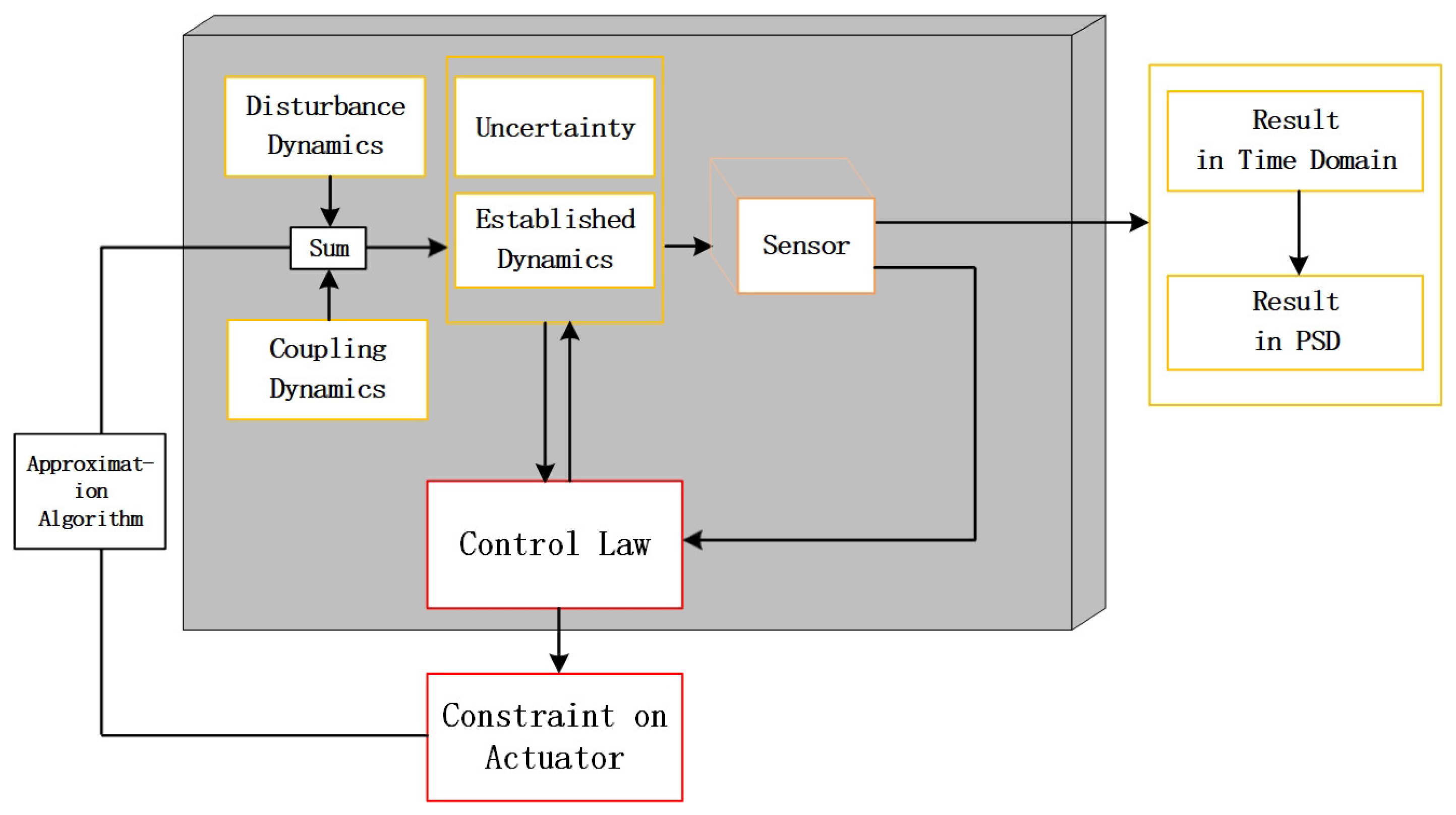
2. Dynamics and Problem Formulation

In this section, we present an analysis of the dynamics for DFAC systems, problems we focused on are formulated, and the background for the TianQin mission is shown in Figure 1. A formation of three geocentric orbit satellites was considered, where $\alpha$ denotes the angle between the spacecraft formation plane and the ecliptic plane, while $\beta$ represents the angle between the detection source RX J0806.3+1527 (a binary white dwarf system) and the ecliptic plane, which remains stable at approximately ${4.7}^{\circ }$. The orbital plane of the spacecraft directly faces the detection source, implying that the line connecting the geocenter and the detection source forms a ${90}^{\circ }-\alpha$ degree angle with respect to the ecliptic plane.

The DFAC system considered in this study comprises five components: two test masses, two cages, and one spacecraft. Each test mass is freely placed on a cage, as shown in Figure 2 and Figure 3. The entire system can be decoupled into several loops, including attitude control loops for the two test masses and one spacecraft, a drag-free control loop for the spacecraft, and suspension loops for the test masses. Consequently, the dynamics of the DFAC system in this study encompass two aspects: drag-free and suspension dynamics representing the offset of test masses within their respective cages and attitude dynamics characterizing the kinematics and dynamics of both the test masses and the spacecraft.

Let us start with the relative motion dynamics between a single test mass and the corresponding enclosure within a spacecraft based on the theory of the dynamics of spacecraft formation [48]. We obtain the following:

$${\mathbf{T}}_O^S{\ddot{\mathbf{r}}}_{OM}=2{\omega }_{\mathbf{S}}\times {\mathbf{T}}_O^S{\dot{\mathbf{r}}}_{MO}+{\dot{\omega }}_S\times ({\mathbf{T}}_O^S{\mathbf{r}}_{MO}+{\mathbf{r}}_{SO})+{\omega }_{\mathbf{S}}\times [{\omega }_{\mathbf{S}}\times ({\mathbf{T}}_O^S{\mathbf{r}}_{MO}+{\mathbf{r}}_{SO})]+({\mathbf{a}}_M^S-{\mathbf{a}}_S)$$

(1)

where ${\omega }_s$ represents the angular velocity of the spacecraft, ${\mathbf{T}}_O^S$ represents the transformation matrix from the cage to the spacecraft, and $({\mathbf{a}}_M^S-{\mathbf{a}}_S)$ represents the different forces between the spacecraft and test masses caused by the environment. Dynamics (1) can be used for both test masses. And in (1), the different forces encompass control signals acting on both the spacecraft and test masses, nonconservative forces exerted on them, gravitational gradient between the spacecraft and each test mass, and stiffness parasitic coupling, and this part can be described as follows:

$${{\mathbf{a}}_M}^{\mathbf{S}}-{\mathbf{a}}_S={\mathbf{f}}_{tm}-{\mathbf{f}}_{sc}+{\mathbf{u}}_{tm}-{\mathbf{u}}_{sc}+\Delta {\mathbf{G}}_{gra}+{\mathbf{F}}_{sti}$$

(2)

In Equation (2), the nonconservative forces acting on the spacecraft are denoted by ${\mathbf{f}}_{sc}$, with solar pressure being the primary influencing factor for ${\mathbf{f}}_{sc}$. The external disturbances on the test masses, represented as ${\mathbf{f}}_{tm}$, arise from residual gas, surface electric charge, temperature fluctuations, cosmic rays, and other factors. It is crucial to limit these disturbances within the required residual acceleration levels. Undoubtedly, this poses a significant hardware-level challenge for deep space missions. The differential gravitational effects $\Delta {\mathbf{G}}_{gra}$ exerted on both the spacecraft and test masses due to stars have a profound impact on this system. Unfortunately, gravitational gradients cannot be compensated for by thrust systems alone. Considering a geocentric background perspective in the TianQin mission, we primarily considered the Earth, Sun, and Moon as the main influencing celestial bodies while disregarding other stars and the $J_2$ perturbations of Earth. The description of the gravitational gradients can be formulated as follows:

$$\Delta {\mathbf{G}}_{gra}=\Delta {\mathbf{G}}_{Earth}+\Delta {\mathbf{G}}_{Sun}+\Delta {\mathbf{G}}_{Moon}$$

(3)

Remark 1.

Considering the orbital background in this study, we conducted a simulation to obtain the effect magnitude of the gravitational gradient on the relative motion. This was achieved by utilizing the parameters and orbital elements of the relevant celestial bodies. The specific outcomes are provided with the following magnitudes: Earth (${10}^{-10}$ m/s²), Moon (${10}^{-13}$ m/s²), Sun (${10}^{-13}$ m/s²), Venus (${10}^{-19}$ m/s²), and Mars (${10}^{-21}$ m/s²). The effects from other factors are even more negligible in magnitude; therefore, further elaboration on them is deemed unnecessary.

The parasitic coupling of the stiffness is represented by ${\mathbf{F}}_{sti}={\mathsf{\Omega }}_{sti}\mathbf{r}$, where ${\mathsf{\Omega }}_{sti}$ denotes the stiffness matrix and $\mathbf{r}$ represents the displacement of the specific test mass within the cavity under discussion, which is influenced by $F_{sti}$. It can be simplified to only include coefficients related to the offset of the test mass [49]. The stiffness matrix was found to have the following properties [43,50]: the dominant factors that contribute to the stiffness coupling matrix are the electromagnetic effect between the actuator and test mass, as well as the self-gravity between the test masses and the spacecraft. Due to this reason, we primarily focused on the diagonal elements since their crosstalk influence order with position vectors on other axes is two orders or more smaller than that of the main shaft system. Therefore, it is crucial for us to consider these diagonal elements. Additionally, based on a deep space background, coefficients in the matrix related to the attitude parameters in dynamics (1) are significantly smaller compared with those in the stiffness matrix [43,49,50]. Therefore, the dynamics of the test masses can be simplified to the form of transfer functions $G_{pm}$ and $G_{am}$, as follows:

$$G_{pm}=\frac{1}{m_m}·\frac{1}{s^2-{\lambda }_{diag}^2}$$

(4)

$$G_{am}=\frac{1}{I_m}·\frac{1}{s^2-{\mu }_{diag}^2}$$

(5)

where ${\lambda }_{diag}^2$ and ${\mu }_{diag}^2$ represent the diagonal elements of the stiffness matrix for the orbit and attitude degrees of freedom, respectively.

It is evident that a single rigid spacecraft cannot simultaneously track two test masses. Therefore, it becomes necessary to select a drag-free reference point that can effectively compensate for the nonconservative forces that act on the spacecraft. This reference point also plays a crucial role in preventing collisions between the test masses and their cages. In this paper, we describe the tracking function for the spacecraft using a selection matrix ${\mathbf{J}}_{tra}$:

$$\left[\begin{array}{c}{\mathbf{r}}_X\\ {\mathbf{r}}_Y\\ {\mathbf{r}}_Z\end{array}\right]={\mathbf{J}}_{\mathbf{tra}}{\left[\begin{array}{cccccc}{\mathbf{r}}_{1X}& {\mathbf{r}}_{1Y}& {\mathbf{r}}_{1Z}& {\mathbf{r}}_{2X}& {\mathbf{r}}_{2Y}& {\mathbf{r}}_{2Z}\end{array}\right]}^T$$

(6)

where ${\left[\begin{array}{cccccc}{\mathbf{r}}_{1X}& {\mathbf{r}}_{1Y}& {\mathbf{r}}_{1Z}& {\mathbf{r}}_{2X}& {\mathbf{r}}_{2Y}& {\mathbf{r}}_{2Z}\end{array}\right]}^T$ represents the offset from the center of mass (CoM) of the test mass to the center of the relevant cage, and ${\left[\begin{array}{ccc}{\mathbf{r}}_X& {\mathbf{r}}_Y& {\mathbf{r}}_Z\end{array}\right]}^T$ represents the tracking targets of the spacecraft. In order to establish an appropriate reference frame for precise tracking in the two-test-mass drag-free system, a transformation matrix is required to convert the six translational degrees of freedom associated with the test masses into three degrees of freedom. Considering the specific demands of the space gravitational wave detection mission, we provide the following drag-free control selection matrix that effectively solves for the center positions of both test masses. And the drag-free control selection matrix can be described as follows:

$${\mathbf{J}}_{tra}=\left[\begin{array}{cccccc}\frac{c\beta }{2}& 0& \frac{s\beta }{2}& \frac{c\beta }{2}& 0& -\frac{s\beta }{2}\\ 0& \frac{1}{2}& 0& 0& \frac{1}{2}& 0\\ -\frac{s\beta }{2}& 0& \frac{c\beta }{2}& \frac{s\beta }{2}& 0& \frac{c\beta }{2}\end{array}\right]$$

(7)

where $\beta$ represents the respiratory angle of the spacecraft formation, where $c\beta :=cos\left(\beta \right)$ and $s\beta :=sin\left(\beta \right)$.

And thus, the dynamics and kinematics of the spacecraft and test masses can be described as follows: We denote the moment of inertia, disturbing torque, and control torque as $\mathbf{J}$, $\mathbf{M}$, and $\mathbf{D}$, respectively, and the subscripts S and $mi$ represent the spacecraft and test masses, respectively. Furthermore, we denote the angular velocity and Euler angle of the test masses as ${\omega }_{mi}$ and ${\left[\begin{array}{ccc}{\phi }_i& {\theta }_i& {\psi }_i\end{array}\right]}^T$, respectively, where $i=1,2$. We propose the following attitude dynamics:

$${\mathbf{J}}_s{\dot{\omega }}_s+{\omega }_s\times {\mathbf{J}}_s{\omega }_s={\mathbf{M}}_s+{\mathbf{D}}_s$$

(8)

$${\mathbf{J}}_{mi}{\dot{\omega }}_{mi}+{\omega }_{mi}\times {\mathbf{J}}_{mi}{\omega }_{mi}={\mathbf{M}}_{mi}+{\mathbf{D}}_{mi}$$

(9)

The attitude kinematics:

$${\omega }_s=\left[\begin{array}{c}{\omega }_{\mathrm{x}}\hfill \\ {\omega }_y\hfill \\ {\omega }_z\hfill \end{array}\right]=\left[\begin{array}{ccc}c{\theta }_s& 0& s{\theta }_s\\ 0& 1& s{\phi }_s\\ s{\theta }_s& 0& c{\theta }_{s}c{\phi }_s\end{array}\right]\left[\begin{array}{c}{\dot{\phi }}_s\hfill \\ {\dot{\theta }}_s\hfill \\ {\dot{\psi }}_s\hfill \end{array}\right]+\left[\begin{array}{c}c{\theta }_{s}s{\psi }_s+s{\phi }_{s}s{\theta }_{s}c{\psi }_s\hfill \\ c{\phi }_{s}c{\psi }_s\hfill \\ s{\theta }_{s}s{\psi }_s-s{\phi }_{s}s{\theta }_{s}c{\psi }_s\hfill \end{array}\right]{\omega }_0$$

(10)

$$\begin{array}{c}{\omega }_{mi}=\left[\begin{array}{c}{\omega }_{\mathrm{ix}}\hfill \\ {\omega }_{iy}\hfill \\ {\omega }_{iz}\hfill \end{array}\right]=\left[\begin{array}{ccc}c{\theta }_i& 0& s{\theta }_i\\ 0& 1& s{\phi }_i\\ s{\theta }_i& 0& c{\theta }_{i}c{\phi }_i\end{array}\right]\left[\begin{array}{c}{\dot{\phi }}_i\hfill \\ {\dot{\theta }}_i\hfill \\ {\dot{\psi }}_i\hfill \end{array}\right]+\left[\begin{array}{c}c{\theta }_{i}s{\psi }_i+s{\phi }_{i}s{\theta }_{i}c{\psi }_i\hfill \\ c{\phi }_{i}c{\psi }_i\hfill \\ s{\theta }_{i}s{\psi }_i-s{\phi }_{i}s{\theta }_{i}c{\psi }_i\hfill \end{array}\right]{\omega }_{0i}\hfill \end{array}$$

(11)

where the scalar values of the angular velocity of the spacecraft and the test mass are denoted by ${\omega }_0$ and ${\omega }_{0i}$, respectively. The process of spacecraft attitude stabilization involves two stages. First, in wide-angle situations, it is crucial to consider the nonlinear dynamics component that cannot be neglected. In the subsequent stage, the micro-thrust system assumes the role of actuation for attitude control. Once this system enters the drag-free science mode, the problem can be described as an error correction for small angles. Based on this scenario, the attitude dynamics of the satellite can be decoupled into three single-input single-output (SISO) systems represented by transfer functions [41]:

$$G_a=\frac{1}{s^2}$$

(12)

Based on the proposed dynamics, we aimed to address the following key objectives in this study:

• Propose a viable allocation scheme for actuators, including thrusters for the satellite and suspension control actuators for the test masses.
• Devise a disturbance estimator for the satellite and establish an output feedback control law for the satellite based on this estimator.
• Design suspension controllers for the test masses, including attitude loop control laws and orbit error modification between the test masses and relevant cages.
• Numerical simulation using a geocentric orbit in the TianQin mission is provided.

3. Main Results

In this section, the main results for the problem we focused on are presented, and the design for the whole DFAC system is analyzed in detail. For the sake of convenience, we denote the two test masses as TM1 and TM2.

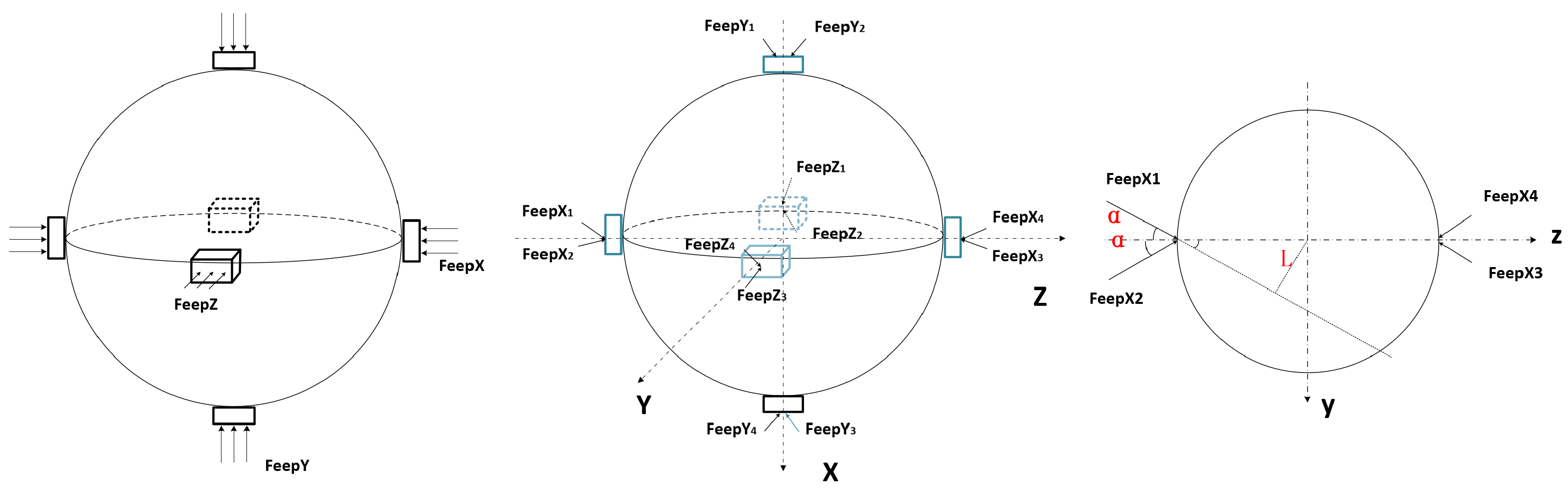
3.1. Actuator System

In the DFAC system, there are three actuation systems responsible for controlling the entire loop: a thrust system for spacecraft propulsion and two electrostatic suspension systems for the test masses. To ensure that each actuation system effectively generates control signals for all six degrees of freedom (three for position and three for attitude), it was imperative to devise an optimization and assignment scheme specifically tailored for the micro-thrust system and suspension systems.

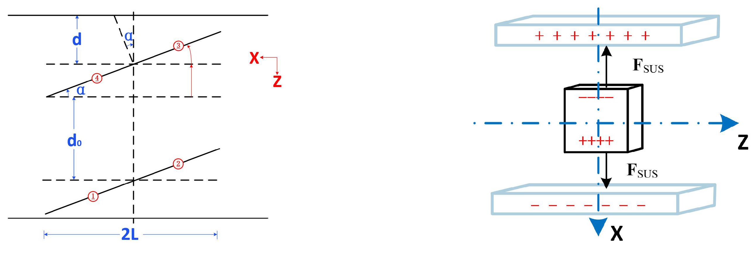
3.1.1. Micro-Thrust System

In this study, we considered SC as a spherical object. For convenience, we designate the field emission electric propulsion (FEEP) as $Fee{p}_{pq}$, where $p=x,y,z$ and $q=1,2,3,4$. Specifically, $Fee{p}_{xq}$ represents the layout in the YOZ plane, $Fee{p}_{yq}$ denotes the layout in the XOZ plane, and $Fee{p}_{zq}$ signifies the layout in the XOY plane. The micro-thrust system comprises a total of 12 thrusters. It was assumed that each thruster is located at a distance of L from the center O. Furthermore, every pair of thrusters exhibits symmetry about their corresponding axis with an angle difference of $2\alpha$. Figure 4 illustrates a schematic diagram depicting this arrangement.

Additionally, we present the allocation matrix for our micro-thrust system in Equation (13), where $c\alpha =cos\left(\alpha \right)$, $s\alpha =sin\left(\alpha \right)$, and ${\left[\begin{array}{cccc}\begin{array}{ccc}{\mathbf{F}}_x& {\mathbf{F}}_y& {\mathbf{F}}_z\end{array}& \mathbf{T}{\mathbf{q}}_x& \mathbf{T}{\mathbf{q}}_y& \mathbf{T}{\mathbf{q}}_z\end{array}\right]}^T$ represents the final control signal on the satellite, including the control force and control torque.

$$\left[\begin{array}{c}{\mathbf{F}}_x\\ {\mathbf{F}}_y\\ {\mathbf{F}}_z\\ \mathbf{T}{\mathbf{q}}_x\\ \mathbf{T}{\mathbf{q}}_y\\ \mathbf{T}{\mathbf{q}}_z\end{array}\right]=\left[\begin{array}{cccccccccccc}0& 0& 0& 0& c\alpha & c\alpha & -c\alpha & -c\alpha & s\alpha & -s\alpha & -s\alpha & s\alpha \\ s\alpha & -s\alpha & -s\alpha & s\alpha & 0& 0& 0& 0& c\alpha & c\alpha & -c\alpha & -c\alpha \\ c\alpha & c\alpha & -c\alpha & -c\alpha & s\alpha & -s\alpha & -s\alpha & s\alpha & 0& 0& 0& 0\\ -L& L& -L& L& 0& 0& 0& 0& 0& 0& 0& 0\\ 0& 0& 0& 0& -L& L& -L& L& 0& 0& 0& 0\\ 0& 0& 0& 0& 0& 0& 0& 0& -L& L& -L& L\end{array}\right]\left[\begin{array}{c}\mathbf{Fee}{\mathbf{p}}_{x1}\\ \mathbf{Fee}{\mathbf{p}}_{x2}\\ \mathbf{Fee}{\mathbf{p}}_{x3}\\ \mathbf{Fee}{\mathbf{p}}_{x4}\\ \mathbf{Fee}{\mathbf{p}}_{y1}\\ \mathbf{Fee}{\mathbf{p}}_{y2}\\ \mathbf{Fee}{\mathbf{p}}_{y3}\\ \mathbf{Fee}{\mathbf{p}}_{y4}\\ \mathbf{Fee}{\mathbf{p}}_{z1}\\ \mathbf{Fee}{\mathbf{p}}_{z2}\\ \mathbf{Fee}{\mathbf{p}}_{z3}\\ \mathbf{Fee}{\mathbf{p}}_{z4}\end{array}\right]$$

(13)

Due to the inherent characteristics of FEEP, it facilitates ion acceleration via an electric field and subsequently achieves the desired thrust through reverse launching. FEEP exhibits reduced propellant consumption while relying more on energy utilization. Consequently, in the optimization process, the allocation of propellant to each group is disregarded, and instead, thrust allocation is optimized with a focus on the total energy consumption. Simultaneously, during the thrust integration design, certain thrusters were selected as redundancy measures whereby they remain idle until other thrusters fail, ensuring continuous operation. In summary, this section encompasses two optimization objectives: minimizing the total energy consumption and determining the number of simultaneously functioning thrusters under long-term observation. To simplify the aforementioned optimization problems, we can consider one thruster idle on each side and introduce redundancy by selecting $Fee{p}_{x4}$, $Fee{p}_{y4}$, and $Fee{p}_{z4}$. The optimal objective can be represented as follows:

$${\mathbf{F}}_{scg}=\sum _{p=1}^3\sum _{q=1}^3∥\mathbf{Fee}{\mathbf{p}}_{pq}∥$$

(14)

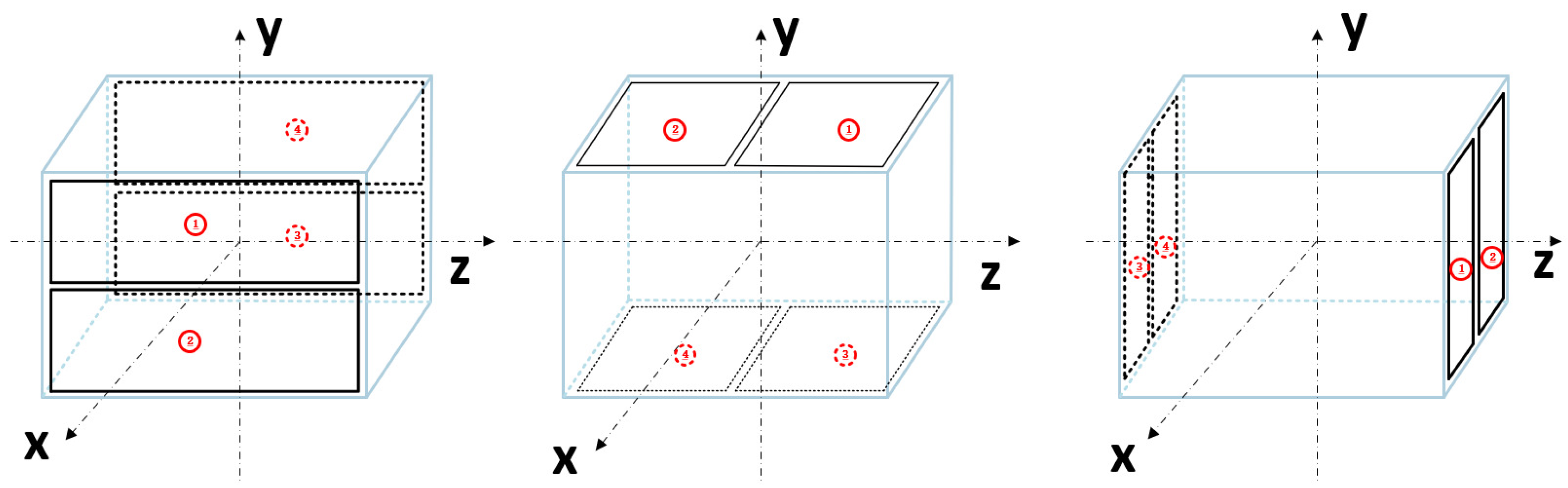
3.1.2. Suspension System

The electrostatic actuator operates by initially applying a voltage to the electrode plate, which then attracts charged particles attached to the test mass. As a result, the test mass acquires an opposite charge to that of the plate.

Figure 5 illustrates the schematic diagram of electrostatic actuators [51,52]. Due to the non-uniformity of the electrostatic field, all calculations pertaining to this component in this article are based on approximate considerations. The allocation of electrostatic actuators for test masses is similar to that of micro-thrust systems, and the allocation matrix can be seen in Equations (15) and (16), while Figure 6 showcases the arrangement of electrostatic actuators.

$$\left[\begin{array}{c}{\mathbf{F}}_{ix}\\ {\mathbf{F}}_{iy}\\ {\mathbf{F}}_{iz}\\ \mathbf{T}{\mathbf{q}}_{ix}\\ \mathbf{T}{\mathbf{q}}_{iy}\\ \mathbf{T}{\mathbf{q}}_{iz}\end{array}\right]=\left[\begin{array}{cccccccccccc}1& 1& -1& -1& 0& 0& 0& 0& 0& 0& 0& 0\\ 0& 0& 0& 0& 1& 1& -1& -1& 0& 0& 0& 0\\ 0& 0& 0& 0& 0& 0& 0& 0& 1& 1& -1& -1\\ -l& l& -l& l& 0& 0& 0& 0& 0& 0& 0& 0\\ 0& 0& 0& 0& -l& l& -l& l& 0& 0& 0& 0\\ 0& 0& 0& 0& 0& 0& 0& 0& -l& l& -l& l\end{array}\right]\left[\begin{array}{c}\mathbf{Su}{\mathbf{s}}_{x1}\\ \mathbf{Su}{\mathbf{s}}_{x2}\\ \mathbf{Su}{\mathbf{s}}_{x3}\\ \mathbf{Su}{\mathbf{s}}_{x4}\\ \mathbf{Su}{\mathbf{s}}_{y1}\\ \mathbf{Su}{\mathbf{s}}_{y2}\\ \mathbf{Su}{\mathbf{s}}_{y3}\\ \mathbf{Su}{\mathbf{s}}_{y4}\\ \mathbf{Su}{\mathbf{s}}_{z1}\\ \mathbf{Su}{\mathbf{s}}_{z2}\\ \mathbf{Su}{\mathbf{s}}_{z3}\\ \mathbf{Su}{\mathbf{s}}_{z4}\end{array}\right]$$

(15)

$$\left\{\begin{array}{ccc}\begin{array}{c}Su{s}_{X1}=\frac{K_C}{{(d_0-r_X-L{\alpha }_Z)}^2}{V_{X1}}^2;\hfill \\ Su{s}_{X2}=\frac{K_C}{{(d_0-r_X+L{\alpha }_Z)}^2}{V_{X2}}^2;\hfill \\ Su{s}_{X3}=\frac{K_C}{{(d_0+r_X-L{\alpha }_Z)}^2}{V_{X3}}^2;\hfill \\ Su{s}_{X4}=\frac{K_C}{{(d_0+r_X+L{\alpha }_Z)}^2}{V_{X4}}^2;\hfill \end{array}& \begin{array}{c}Su{s}_{Y1}=\frac{K_C}{{(d_0-r_Y-L{\alpha }_X)}^2}{V_{Y1}}^2;\hfill \\ Su{s}_{Y2}=\frac{K_C}{{(d_0-r_Y+L{\alpha }_X)}^2}{V_{Y2}}^2;\hfill \\ Su{s}_{Y3}=\frac{K_C}{{(d_0+r_Y-L{\alpha }_X)}^2}{V_{Y3}}^2;\hfill \\ Su{s}_{Y4}=\frac{K_C}{{(d_0+r_Y+L{\alpha }_X)}^2}{V_{Y4}}^2;\hfill \end{array}& \begin{array}{c}Su{s}_{Z1}=\frac{K_C}{{(d_0-r_Z-L{\alpha }_Y)}^2}{V_{Z1}}^2.\hfill \\ Su{s}_{Z2}=\frac{K_C}{{(d_0-r_Z+L{\alpha }_Y)}^2}{V_{Z2}}^2.\hfill \\ Su{s}_{Z3}=\frac{K_C}{{(d_0+r_Z-L{\alpha }_Y)}^2}{V_{Z3}}^2.\hfill \\ Su{s}_{Z4}=\frac{K_C}{{(d_0+r_Z+L{\alpha }_Y)}^2}{V_{Z4}}^2.\hfill \end{array}\end{array}\right.$$

(16)

In (15) and (16), ${\left[\begin{array}{cccc}\begin{array}{ccc}{\mathbf{F}}_{ix}& {\mathbf{F}}_{iy}& {\mathbf{F}}_{iz}\end{array}& \mathbf{T}{\mathbf{q}}_{ix}& \mathbf{T}{\mathbf{q}}_{iy}& \mathbf{T}{\mathbf{q}}_{iz}\end{array}\right]}^T$ represents the final control signal on the test masses, including the control force and control torque. $c=X,Y,Z$ and $d=1,2,3,4$ represent the control force in the suspension loop, and $V{s}_{ij}$ represents the output of electrode plate. And we have $K_C=4{\epsilon }_0{a}_0{b}_0$, where $a_0$ and $b_0$ represent the parameters of the plate size, and ${\epsilon }_0$ represents the permittivity of a vacuum. Here, we assumed $sin{\alpha }_Y\approx {\alpha }_Y$ based on the micro-rotation, and $4l$ represents the length of the plate.

3.2. Predictive Controllers Design for the Spacecraft

For a nominal plant $G_p=-\frac{1}{m_s}·\frac{1}{s^2-{\lambda }_{diag}^2}$ and $G_a=\frac{1}{s^2}$, they can be transformed into a form of the discrete state space as in (17), and the sampling interval is recorded as h:

$$\begin{array}{cc}\hfill & \Delta \mathbf{z}(k+1)={\mathbf{A}}_h\Delta \mathbf{z}\left(k\right)+{\mathbf{B}}_h\Delta \mathbf{u}\left(k\right)\hfill \\ \hfill & \Delta \mathbf{y}\left(k\right)=\left[{\mathbf{C}}_h\right]\Delta \mathbf{z}\left(k\right)\hfill \end{array}$$

(17)

Define ${\widehat{\mathsf{ȷ}}}_s={\left[\begin{array}{ccc}{\widehat{\mathsf{ȷ}}}_{s1}& {\widehat{\mathsf{ȷ}}}_{s2}& {\widehat{\mathsf{ȷ}}}_{s3}\end{array}\right]}^T$ as the estimation of the translation state of the vector from the CoM of the SC to the drag-free reference point, ${\widehat{\mathsf{Ø}}}_s={\left[\begin{array}{ccc}{\widehat{\mathsf{Ø}}}_{s1}& {\widehat{\mathsf{Ø}}}_{s2}& {\widehat{\mathsf{Ø}}}_{s3}\end{array}\right]}^T$ is the estimation of attitude state of SC, and the extended observer is proposed as follows [53]: The estimator of the spacecraft-tracking plant can be described as

$${\widehat{\mathsf{ȷ}}}_s(k+1)={\mathbf{A}}_{sp}{\widehat{\mathsf{ȷ}}}_s\left(k\right)+{\mathbf{B}}_{sp}{\mathbf{u}}_{so}\left(k\right)+{\mathbf{L}}_{sp}({\mathbf{z}}_1\left(k\right)-{\widehat{\mathsf{ȷ}}}_{s1}\left(k\right))$$

(18)

and the estimator of the attitude state of the satellite can be described as

$${\widehat{\mathsf{Ø}}}_s(k+1)={\mathbf{A}}_{sa}{\widehat{\mathsf{Ø}}}_s\left(k\right)+{\mathbf{B}}_{sa}{\mathbf{u}}_{ao}\left(k\right)+{\mathbf{L}}_{sa}({\mathbf{z}}_{sa1}\left(k\right)-{\widehat{\mathsf{Ø}}}_{\mathbf{s}\mathbf{1}}\left(k\right))$$

(19)

where ${\mathbf{L}}_{sp}$ and ${\mathbf{L}}_{sa}$ are the gains of the drag-free observer and attitude observer for the satellite, respectively, and we obtain ${\mathbf{A}}_{sp}={\mathbf{A}}_{sa}=\left[\begin{array}{ccc}{\mathbf{I}}_{3\times 3}& \mathbf{T}{\mathbf{I}}_{\mathbf{3}\times \mathbf{3}}& {\mathbf{0}}_{3\times 3}\\ {\mathbf{0}}_{3\times 3}& {\mathbf{I}}_{3\times 3}& {\mathbf{0}}_{3\times 3}\\ {\mathbf{0}}_{3\times 3}& {\mathbf{0}}_{3\times 3}& {\mathbf{I}}_{3\times 3}\end{array}\right]$, ${\mathbf{B}}_{sp}=\left[\begin{array}{c}{\mathbf{0}}_{3\times 3}\\ -\frac{1}{m_S}\mathbf{T}{\mathbf{I}}_{\mathbf{3}\times \mathbf{3}}\\ {\mathbf{0}}_{3\times 3}\end{array}\right]$, and ${\mathbf{B}}_{sp}=\left[\begin{array}{c}{\mathbf{0}}_{3\times 3}\\ {{\mathbf{I}}_S}^{-1}\mathbf{T}{\mathbf{I}}_{\mathbf{3}\times \mathbf{3}}\\ {\mathbf{0}}_{3\times 3}\end{array}\right]$ in (18) and (19). Based on ADRC theory [53], ${\mathbf{u}}_{sp}$ is the real control signal for SC, ${\mathbf{u}}_{so}$ is the feedback for the observer (18), and $\frac{{\widehat{\mathsf{ȷ}}}_{s3}}{m_s}$ is the compensation for the disturbance of the drag-free system due to the extended state, and their equation is described as

$${\mathbf{u}}_{sp}={\mathbf{u}}_{so}-\frac{{\widehat{\mathsf{ȷ}}}_{s3}}{m_s}$$

(20)

And then, we define the value function of the drag-free loop as the performance output ${\widehat{\mathbf{y}}}_c$:

$${\widehat{\mathbf{y}}}_c={\mathbf{C}}_s{\left[\begin{array}{ccc}{\widehat{\mathsf{ȷ}}}_{s1}& {\widehat{\mathsf{ȷ}}}_{s2}& {\widehat{\mathsf{ȷ}}}_{s3}\end{array}\right]}^T=\left[\begin{array}{ccc}{\lambda }_1& {\lambda }_2& {\lambda }_3\end{array}\right]{\left[\begin{array}{ccc}{\widehat{\mathsf{ȷ}}}_{s1}& {\widehat{\mathsf{ȷ}}}_{s2}& {\widehat{\mathsf{ȷ}}}_{s3}\end{array}\right]}^T$$

(21)

where ${\lambda }_1$, ${\lambda }_2$, and ${\lambda }_3$ are some positive constants. In [54], the gain can be set as the bandwidth of the observer. Taking the x-axis as an example, the bandwidth of the observer is denoted as ${\omega }_{cx}$, and we obtain

$${\mathbf{L}}_{sp}=\left[\begin{array}{ccc}{\mathsf{\ae }}_{\mathbf{x}}& & \\ & {\mathsf{\ae }}_{\mathbf{y}}& \\ & & {\mathsf{\ae }}_{\mathbf{z}}\end{array}\right],{\mathsf{\ae }}_x=\left[\begin{array}{ccc}3·{\omega }_{\mathrm{cx}}& 0& 0\\ 3·{\omega }_{\mathrm{cx}}·{\omega }_{\mathrm{cx}}& 0& 0\\ {{\omega }_{\mathrm{cx}}}^3& 0& 0\end{array}\right]$$

(22)

As is different from the suspension loop, the micro-thrust system of the satellite has the constraint of the output frequency; it is difficult for us to provide a control signal above 2 Hz in the frequency domain. Therefore, a drag-free loop is considered with the optimal problem as

$$\mathbf{J}=\left[\begin{array}{cccccc}1& 1& 1& \cdots & 1& 1\\ 0& 1& 1& \cdots & 1& 1\\ 0& 0& 1& \cdots & 1& 1\\ & & & \ddots & & \\ 0& 0& 0& \cdots & 1& 1\\ 0& 0& 0& \cdots & 0& 1\end{array}\right]\left[\begin{array}{c}{∥{\widehat{\mathbf{y}}}_c(k+1|k)-{\mathbf{R}}_{sp}(k+1)∥}^2\hfill \\ {∥{\widehat{\mathbf{y}}}_c(k+2|k)-{\mathbf{R}}_{sp}(k+2)∥}^2\hfill \\ \dots \hfill \\ {∥{\widehat{\mathbf{y}}}_c(k+p|k)-{\mathbf{R}}_{sp}(k+i)∥}^2\hfill \end{array}\right]$$

(23)

where ${\mathbf{R}}_{sp}\left(k\right)$ represents the tracking target at the time k, and $∥·∥$ represents the Euclidean norm. In (23), we use a predictive control problem instead of the optical problem, considering the foregoing constraints: (i). the predictive horizon is equal to the control horizon, we mark them as p; (ii). the control output $\mathbf{u}$ remains unchanged in each time interval. In this way, the problem is transformed into an optimal control problem in one control domain, and the estimator of the drag-free loop in one control domain is as follows:

$$\Delta {\widehat{\mathsf{ȷ}}}_s(k+p|k)={{\mathbf{A}}_{sp}}^p\Delta {\widehat{\mathsf{ȷ}}}_s\left(k\right)+\sum _{i=0}^{p-1}{{\mathbf{A}}_{sp}}^{p-i-1}{\mathbf{B}}_{sp}\Delta {\mathbf{u}}_{so}(k+i)+\sum _{i=0}^{p-1}{{\mathbf{A}}_{sp}}^{p-i-1}{\mathbf{L}}_{sp}{\mathbf{e}}_s(k+i)$$

(24)

By choosing the performance output ${\widehat{\mathbf{y}}}_{\mathbf{c}}$, the tracking controller hopes that it can obtain the balance of the relative motion and relative velocity between spacecraft and the reference point. And the optimal problem is described in (25) and (26). For the sake of convenience, ${\mathbf{S}}_{so}=\left[\begin{array}{c}{\mathbf{C}}_s{\mathbf{A}}_{sp}\hfill \\ {\displaystyle \sum _{i=1}^2}{\mathbf{C}}_s{{\mathbf{A}}_{sp}}^i\hfill \\ \dots \hfill \\ {\displaystyle \sum _{i=1}^p}{\mathbf{C}}_s{{\mathbf{A}}_{sp}}^i\hfill \end{array}\right]$ and ${\mathbf{S}}_{su}=\left[\begin{array}{c}{\mathbf{C}}_s{\mathbf{B}}_{sp}\\ {\mathbf{C}}_s{\mathbf{A}}_{sp}{\mathbf{B}}_{sp}\\ \dots \\ {\mathbf{C}}_s{{\mathbf{A}}_{sp}}^{i-1}{\mathbf{B}}_{sp}\end{array}\right]$ denote the states of the observer and input signals, and we denote ${\mathbf{S}}_{se}=\left[\begin{array}{c}{\mathbf{C}}_s{\mathbf{L}}_{sp}\Delta {\mathbf{e}}_s\left(k\right)\\ {\displaystyle \sum _{i=0}^1}{\displaystyle \sum _{\mathrm{j}=1}^{i+1}}{\mathbf{C}}_s{\mathbf{L}}_s{{\mathbf{A}}_{sp}}^{j-1}{\mathbf{B}}_{sp}\Delta {\mathbf{e}}_s(k+1-i)\\ \dots \\ {\displaystyle \sum _{i=0}^{p-1}}{\displaystyle \sum _{\mathrm{j}=1}^{i+1}}{\mathbf{C}}_s{\mathbf{L}}_s{{\mathbf{A}}_{sp}}^{j-1}{\mathbf{B}}_{sp}\Delta {\mathbf{e}}_s(k+p-1-i)\end{array}\right]$ as the matrix of the estimation error. The performance function

$$\begin{array}{cc}\hfill & {\mathbf{g}}_s-\left[\begin{array}{c}{\widehat{\mathbf{y}}}_s\left(k\right)-{\mathbf{R}}_{sp}(k+1)\hfill \\ {\widehat{\mathbf{y}}}_s\left(k\right)-{\mathbf{R}}_{sp}(k+2)\hfill \\ \dots \hfill \\ {\widehat{\mathbf{y}}}_s\left(k\right)-{\mathbf{R}}_{sp}(k+i)\hfill \end{array}\right]=\left[\begin{array}{c}{\mathbf{C}}_s{\mathbf{A}}_{sp}\Delta {\widehat{\mathsf{ȷ}}}_s\left(k\right)+{\mathbf{C}}_s{\mathbf{B}}_{sp}\Delta {\mathbf{u}}_{so}\left(k\right)+{\mathbf{C}}_s{\mathbf{L}}_{sp}\Delta {\mathbf{e}}_s\left(k\right)\\ {\mathbf{C}}_s({\mathbf{A}}_{sp}+{{\mathbf{A}}_{sp}}^2)\Delta {\widehat{\mathsf{ȷ}}}_s\left(k\right)+{\mathbf{C}}_s{\mathbf{A}}_{sp}{\mathbf{B}}_{sp}\Delta {\mathbf{u}}_{so}\left(k\right)+{\displaystyle \sum _{i=0}^1}{\displaystyle \sum _{\mathrm{j}=1}^{i+1}}{\mathbf{C}}_s{{\mathbf{A}}_{sp}}^{j-1}{\mathbf{B}}_{sp}\Delta {\mathbf{e}}_s(k+1-i)\\ \dots \\ {\displaystyle \sum _{i=1}^p}{\mathbf{C}}_s{{\mathbf{A}}_{sp}}^i\Delta {\widehat{\mathsf{ȷ}}}_s\left(k\right)+{\mathbf{C}}_{\mathbf{s}}{{\mathbf{A}}_{sp}}^{i-1}{\mathbf{B}}_{sp}\Delta {\mathbf{u}}_{so}\left(k\right)+{\displaystyle \sum _{i=0}^{p-1}}{\displaystyle \sum _{\mathrm{j}=1}^{i+1}}{\mathbf{C}}_s\mathbf{L}{{\mathbf{A}}_{sp}}^{j-1}{\mathbf{B}}_{sp}\Delta {\mathbf{e}}_s(k+p-1-i)\end{array}\right]\hfill \\ \hfill & =\left[\begin{array}{c}{\mathbf{C}}_s{\mathbf{B}}_{sp}\\ {\mathbf{C}}_s{\mathbf{A}}_{sp}{\mathbf{B}}_{sp}\\ \dots \\ {\mathbf{C}}_s{{\mathbf{A}}_{sp}}^{i-1}{\mathbf{B}}_{sp}\end{array}\right]\Delta {\mathbf{u}}_{so}\left(k\right)+\left[\begin{array}{c}{\mathbf{C}}_s{\mathbf{A}}_{sp}\Delta {\widehat{\mathsf{ȷ}}}_s\left(k\right)+{\mathbf{C}}_s{\mathbf{L}}_{sp}\Delta {\mathbf{e}}_s\left(k\right)\\ {\mathbf{C}}_s({\mathbf{A}}_{sp}+{{\mathbf{A}}_{sp}}^2)\Delta {\widehat{\mathsf{ȷ}}}_s\left(k\right)+{\displaystyle \sum _{i=0}^1}{\displaystyle \sum _{\mathrm{j}=1}^{i+1}}{\mathbf{C}}_s{{\mathbf{A}}_{sp}}^{j-1}{\mathbf{B}}_{sp}\Delta {\mathbf{e}}_s(k+1-i)\\ \dots \\ {\displaystyle \sum _{i=1}^p}{\mathbf{C}}_{\mathbf{s}}{{\mathbf{A}}_{sp}}^i\Delta {\widehat{\mathsf{ȷ}}}_s\left(k\right)+{\displaystyle \sum _{i=0}^{p-1}}{\displaystyle \sum _{\mathrm{j}=1}^{i+1}}{\mathbf{C}}_s{{\mathbf{A}}_{sp}}^{j-1}{\mathbf{B}}_{sp}\Delta {\mathbf{e}}_s(k+p-1-i)\end{array}\right]\hfill \end{array}$$

(25)

${\mathbf{g}}_s=\left[\begin{array}{c}{\widehat{\mathbf{y}}}_c(k+1|k)-{\mathbf{R}}_{sp}(k+1)\hfill \\ {\widehat{\mathbf{y}}}_c(k+2|k)-{\mathbf{R}}_{sp}(k+2)\hfill \\ \dots \hfill \\ {\widehat{\mathbf{y}}}_c(k+p|k)-{\mathbf{R}}_{sp}(k+i)\hfill \end{array}\right]$ is the symbol for performance for simplification. And the optimal goal is

$$\underset{\Delta {\mathbf{u}}_{\mathbf{so}}\left(k\right)}{min}{\left({\mathbf{S}}_{su}\Delta {\mathbf{u}}_{so}\left(k\right)-{\mathbf{S}}_p(k+1|k)\right)}^T\left({\mathbf{S}}_{su}\Delta {\mathbf{u}}_{so}\left(k\right)-{\mathbf{S}}_p(k+1|k)\right)$$

(26)

And the control law for the drag-free loop is as follows:

$$\Delta {\mathbf{u}}_{so}\left(k\right)={\left({{\mathbf{S}}_{su}}^{\mathrm{T}}{\mathbf{S}}_{su}\right)}^{-1}{{\mathbf{S}}_{su}}^{\mathrm{T}}{\mathbf{S}}_p(k+1|k)$$

(27)

And then we obtain

$$\Delta {\mathbf{u}}_{so}\left(k\right)={({\left[\begin{array}{c}{\mathbf{C}}_s{\mathbf{B}}_{sp}\\ {\mathbf{C}}_s{\mathbf{A}}_{sp}{\mathbf{B}}_{sp}\\ \dots \\ {\mathbf{C}}_s{{\mathbf{A}}_{sp}}^{i-1}{\mathbf{B}}_{sp}\end{array}\right]}^{\mathrm{T}}\left[\begin{array}{c}{\mathbf{C}}_s{\mathbf{B}}_{sp}\\ {\mathbf{C}}_s{\mathbf{A}}_{sp}{\mathbf{B}}_{sp}\\ \dots \\ {\mathbf{C}}_s{{\mathbf{A}}_{sp}}^{i-1}{\mathbf{B}}_{sp}\end{array}\right])}^{-1}{\left[\begin{array}{c}{\mathbf{C}}_s{\mathbf{B}}_{sp}\\ {\mathbf{C}}_s{\mathbf{A}}_{sp}{\mathbf{B}}_{sp}\\ \dots \\ {\mathbf{C}}_s{{\mathbf{A}}_{sp}}^{i-1}{\mathbf{B}}_{sp}\end{array}\right]}^{\mathrm{T}}({\mathbf{R}}_{sp}(k+1)-{\mathbf{S}}_{so}\Delta \mathsf{ȷ}-{\Gamma }_{\mathrm{p}\times 1}{\widehat{\mathbf{y}}}_c\left(k\right)-{\mathbf{S}}_{se})$$

(28)

Because of the convergence of the observer, we can neglect the compensation for the error of the observer in the design, and a weight coefficient, which is denoted by $\mathbf{W}$, was adopted to adjust the gain of controller in (29):

$$\Delta {\mathbf{u}}_{so}\left(k\right)=\mathbf{W}{({\left[\begin{array}{c}{\mathbf{C}}_s{\mathbf{B}}_{sp}\\ {\mathbf{C}}_s{\mathbf{A}}_{sp}{\mathbf{B}}_{sp}\\ \dots \\ {\mathbf{C}}_s{{\mathbf{A}}_{sp}}^{i-1}{\mathbf{B}}_{sp}\end{array}\right]}^{\mathrm{T}}\left[\begin{array}{c}{\mathbf{C}}_s{\mathbf{B}}_{sp}\\ {\mathbf{C}}_s{\mathbf{A}}_{sp}{\mathbf{B}}_{sp}\\ \dots \\ {\mathbf{C}}_s{{\mathbf{A}}_{sp}}^{i-1}{\mathbf{B}}_{sp}\end{array}\right])}^{-1}{\left[\begin{array}{c}{\mathbf{C}}_s{\mathbf{B}}_{sp}\\ {\mathbf{C}}_s{\mathbf{A}}_{sp}{\mathbf{B}}_{sp}\\ \dots \\ {\mathbf{C}}_s{{\mathbf{A}}_{sp}}^{i-1}{\mathbf{B}}_{sp}\end{array}\right]}^{\mathrm{T}}({\mathbf{R}}_{sp}(k+1)-{\mathbf{S}}_{\mathrm{so}}\Delta {\mathsf{ȷ}}_{\mathbf{s}}-{\Gamma }_{\mathrm{p}\times 1}{\widehat{\mathbf{y}}}_c\left(k\right))$$

(29)

$$\Delta {\mathbf{u}}_{sa}\left(k\right)={\mathbf{W}}_a{({\left[\begin{array}{c}{\mathbf{C}}_a{\mathbf{B}}_{sa}\\ {\mathbf{C}}_a{\mathbf{A}}_{sa}{\mathbf{B}}_{sa}\\ \dots \\ {\mathbf{C}}_a{{\mathbf{A}}_{sa}}^{i-1}{\mathbf{B}}_{sa}\end{array}\right]}^{\mathrm{T}}\left[\begin{array}{c}{\mathbf{C}}_a{\mathbf{B}}_{sa}\\ {\mathbf{C}}_a{\mathbf{A}}_{sa}{\mathbf{B}}_{sa}\\ \dots \\ {\mathbf{C}}_a{{\mathbf{A}}_{sa}}^{i-1}{\mathbf{B}}_{sa}\end{array}\right])}^{-1}{\left[\begin{array}{c}{\mathbf{C}}_a{\mathbf{B}}_{sa}\\ {\mathbf{C}}_a{\mathbf{A}}_{sa}{\mathbf{B}}_{sa}\\ \dots \\ {\mathbf{C}}_a{{\mathbf{A}}_{sa}}^{i-1}{\mathbf{B}}_{sa}\end{array}\right]}^{\mathrm{T}}({\mathbf{R}}_a(k+1)-{\mathbf{S}}_{\mathrm{a}}\Delta {\mathbf{Z}}_a-{\Gamma }_{\mathrm{p}\times 1}{\widehat{\mathbf{y}}}_c\left(k\right))$$

(30)

And the attitude controller is similar to the drag-free controller, the controller is described in (30), and ${\mathbf{W}}_a$ is determined by the bandwidth of the attitude loop.

3.3. Output Feedback Control for Suspension Loop

It is difficult for one rigid spacecraft to track two different test masses, and one necessary project concerns the control law for the test masses along insensitive axes, which can help the tracking system obtain the balance between the spacecraft and test masses. In this section, a feedback control law for the suspension loop is proposed; this control law should be a feasible controller for all stiffnesses from $-{10}^{-6}$ to ${10}^{-6}$, and thus, we can use the same controller for two test masses. Take TM1 as the example:

Here, we assume ${\mathbf{W}}_1={\mathit{\rho }}_s$ and ${\mathbf{W}}_2=\frac{1}{\mathrm{s}+0.1}$ as the weight matrices for the suspension loop so as to simplify the problem. The nominal plant can be described as follows:

$${\mathbf{G}}_{\mathrm{nominal}}={\mathbf{W}}_2·{\mathbf{G}}_{\mathrm{M}}·{\mathbf{W}}_1$$

(31)

The open loop and closed loop can be described as follows:

$$\mathbf{L}\left(s\right)={\mathbf{W}}_1·{\mathbf{G}}_{\mathrm{M}}\left(s\right)·{\mathbf{u}}_{mk}·{\mathbf{W}}_2$$

(32)

$${\mathbf{C}}_{\mathrm{M}}\left(s\right)=\frac{{\mathbf{G}}_{\mathrm{M}}\left(s\right)}{{\mathrm{m}}_{\mathrm{TM}}+{\mathbf{u}}_{\mathrm{m}}\left(s\right){\mathbf{G}}_{\mathrm{M}}\left(s\right)}$$

(33)

The optimal problem for the suspension loop can be described as

$$\frac{1}{\epsilon }=\min {∥\left[\begin{array}{c}{\mathbf{G}}_M\\ \mathbf{I}\end{array}\right]{(\mathbf{I}-{\mathbf{u}}_{mk}{\mathbf{G}}_M)}^{-1}\left[\begin{array}{cc}{\mathbf{u}}_{mk}& -\mathbf{I}\end{array}\right]∥}_{\infty }$$

(34)

And then, the control law for the suspension loop is obtained:

$${\mathbf{u}}_{\mathrm{m}}={\mathbf{W}}_2·{\mathbf{u}}_{\mathrm{sus}}·{\mathbf{W}}_1$$

(35)

And thus, we have the control law.

3.4. Control Law for Attitude Loops of Test Masses

The purpose of attitude loops of test masses is to compensate for the attitude deviation. Based on Equations (26) and (27), we can choose the quadratic optimization as the solution of attitude controller for test masses:

$${\mathbf{J}}_{sa}=\sum _{i=1}^p{∥{\mathbf{y}}_{sa}(k+i|k)-{\mathbf{R}}_{sa}(k+i)∥}^2$$

(36)

and make the following definition:

$${\mathbf{S}}_r={\mathbf{R}}_m(k+1)-\left[\begin{array}{c}{\mathbf{C}}_{mz}{\mathbf{A}}_{mz}\hfill \\ {\displaystyle \sum _{i=1}^2}{\mathbf{C}}_{mz}{{\mathbf{A}}_{mz}}^i\hfill \\ \dots \hfill \\ {\displaystyle \sum _{i=1}^p}{\mathbf{C}}_{mz}{{\mathbf{A}}_{mz}}^i\hfill \end{array}\right]\Delta \mathbf{Z}-\Gamma {\widehat{\mathbf{y}}}_{mc}\left(k\right)$$

(37)

where ${\mathbf{A}}_{mz}$, ${\mathbf{B}}_{mz}$, and ${\mathbf{C}}_{mz}$ are the coefficient matrices of the attitude dynamics. The controller can be described as follows:

$$\Delta {\mathbf{u}}_{ma}\left(k\right)={\mathbf{W}}_m{\mathbf{I}}_{5\times 5}{{\mathbf{S}}_{ma}}^T{\mathbf{S}}_{ma}{{\mathbf{S}}_{ma}}^T{\mathbf{S}}_r$$

(38)

where ${\mathbf{S}}_{ma}=\left[\begin{array}{cccc}{\mathbf{C}}_{mz}{\mathbf{B}}_{mu}& 0& \cdots & 0\\ {\displaystyle \sum _{i=1}^2}{\mathbf{C}}_{mz}{{\mathbf{A}}_{mu}}^{i-1}{\mathbf{B}}_{mu}& {\mathbf{C}}_{mz}{\mathbf{B}}_{mu}& \cdots & 0\\ & & \ddots & \\ {\displaystyle \sum _{i=1}^p}{\mathbf{C}}_{mz}{{\mathbf{A}}_{mu}}^{i-1}{\mathbf{B}}_{mu}& {\displaystyle \sum _{i=1}^{p-1}}{\mathbf{C}}_{mz}{{\mathbf{A}}_{mu}}^{i-1}{\mathbf{B}}_{mu}& \cdots & {\mathbf{C}}_{mz}{\mathbf{B}}_{mu}\end{array}\right]$, and ${\mathbf{W}}_m$ has a similar role as ${\mathbf{W}}_a$ in Equation (30) in Section 3.2.

3.5. DC Compensation

Because of the gravity gradient caused by the Earth, Sun, and Moon between the spacecraft and each test mass, there will be some relative motion that can hardly be compensated for by the controller, which is the reason why we need DC (direct current) compensation. The value of the DC signal can be estimated by accelerometers or observers; it is obvious that the DC signal will have a great effect on limiting the offset of the test masses.

In this subsection, the designed estimator is presented as an extended state observer for the states of each test mass:

$$\left\{\begin{array}{c}{\mathbf{e}}_{\mathrm{mi}}={\mathbf{r}}_{\mathrm{mi}}-{\mathbf{z}}_{\mathrm{mi}1}\hfill \\ {\mathbf{z}}_{\mathrm{mi}2}={\dot{\mathbf{z}}}_{\mathrm{mi}1}-{\mathbf{fi}}_{\mathrm{mi}1}({\mathbf{r}}_{\mathrm{mi}}-{\mathbf{z}}_{\mathrm{mi}1})\hfill \\ {\mathbf{z}}_{\mathrm{mi}3}={\dot{\mathbf{z}}}_{\mathrm{mi}2}-{\mathbf{fi}}_{\mathrm{mmi}2}({\mathbf{r}}_{\mathrm{mi}}-{\mathbf{z}}_{\mathrm{mi}1})-\mathbf{Du}\hfill \\ {\dot{\mathbf{z}}}_{\mathrm{mi}3}={\mathbf{fi}}_{\mathrm{mi}3}({\mathbf{r}}_{\mathrm{mi}}-{\mathbf{z}}_{\mathrm{mi}1})\hfill \\ {\mathbf{y}}_{obvi}={\mathbf{z}}_{\mathrm{mi}3}\hfill \end{array}\right.$$

(39)

where $i=1,2$ and ${\mathbf{fi}}_{\mathrm{mmi}1}$, ${\mathbf{fi}}_{\mathrm{mmi}2}$, and ${\mathbf{fi}}_{\mathrm{mmi}3}$ represent the gains of the observers.

The estimation of the disturbance by (39) converges over time, and the constant of the DC signal is determined by the state ${\mathbf{z}}_{\mathrm{mi}3}$.

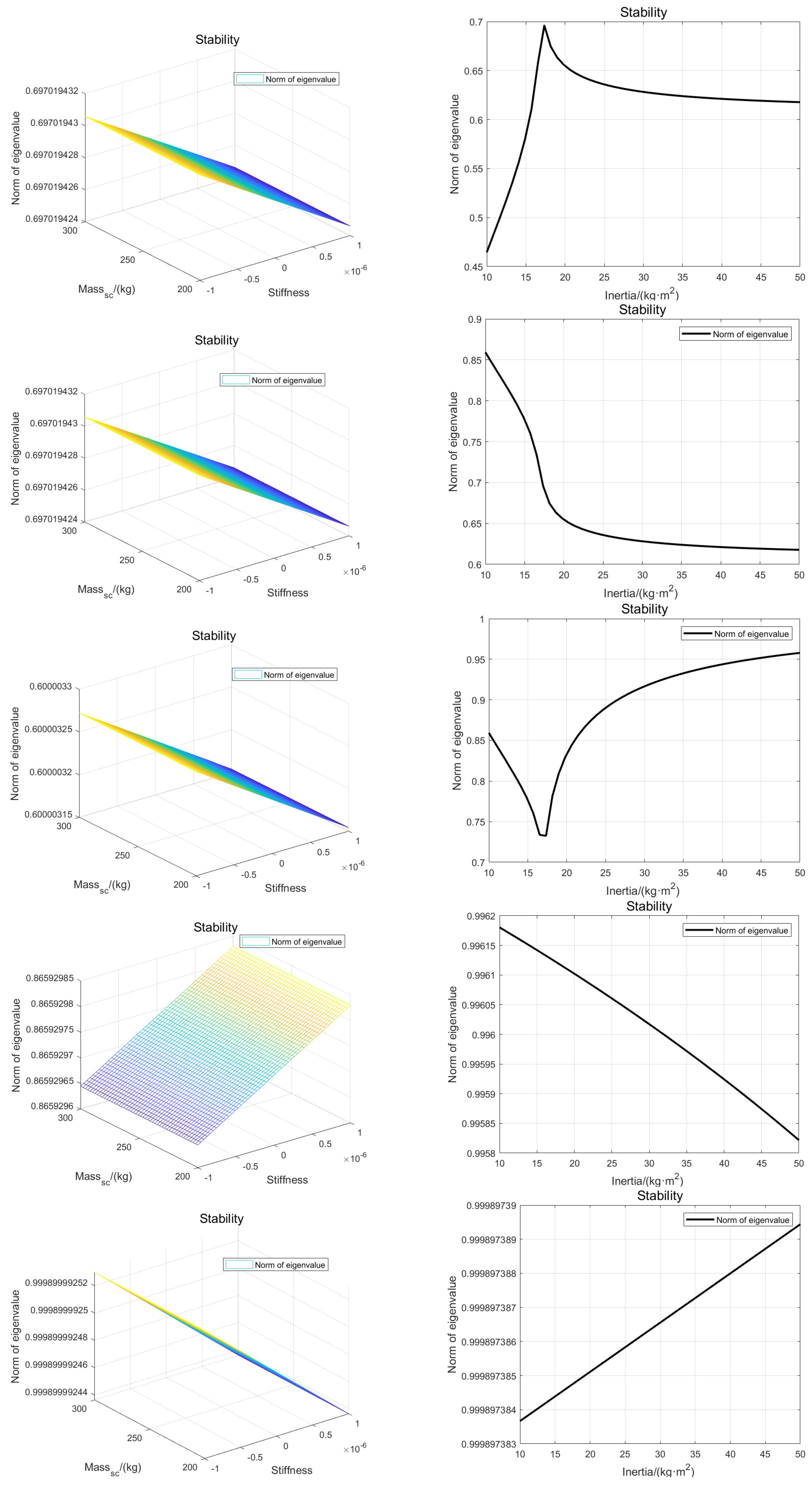
3.6. Stability Analysis

The stability of the control system is analyzed in each loop [41]. In this paper, stability is placed in the discussion with the uncertainty of parameters in (40), including $\Delta m_S$ (the mass of the spacecraft), $\Delta m_m$ (the mass of the test mass), $\Delta I_S$ (the moment of inertia of the spacecraft), and $\Delta {{\lambda }_{diag}}^2$ (the corresponding main diagonal elements of the stiffness matrix):

$$\begin{array}{c}10\mathrm{Nm}\le {\mathrm{I}}_S\le 50\mathrm{Nm}\\ 200\mathrm{kg}\le {\mathrm{m}}_S\le 300\mathrm{kg}\\ 1\mathrm{kg}\le {\mathrm{m}}_m\le 2\mathrm{kg}\\ -1\times {10}^{-6}\le {{\lambda }_{diag}}^2\le 1\times {10}^{-6}\end{array}$$

(40)

And we analyze the stability in two parts: (i) The stability for the suspension loop is given by the pole of (33), which should be assigned at the left half of the complex plane; this feedback loop is stabilized with the uncertainty of parameters $\Delta m_m$ and $\Delta {{\lambda }_{diag}}^2$, and the real part of the pole of (33) is shown in Figure 7.

(ii) The stability for the drag-free loop and attitude loop of the satellite and test masses is given by the eigenvalue of the close loop. Here, we take the drag-free loop as the example. The plant (17), observer (18), and controller (27) comprise the whole drag-free loop, and thus, we can establish new state variables:

$$\xi ={\left[\begin{array}{ccccc}{\mathbf{z}}_1& {\mathbf{z}}_2& {\widehat{\mathsf{ȷ}}}_{11}& {\widehat{\mathsf{ȷ}}}_{12}& {\widehat{\mathsf{ȷ}}}_{13}\end{array}\right]}^T$$

(41)

the controller is marked as

$$\left\{\begin{array}{c}\Delta {\mathbf{u}}_{so}\left(k\right)=-{\mathbf{U}}_1\Delta {\widehat{\mathsf{ȷ}}}_s\left(k\right)-{\mathbf{U}}_2{\widehat{\mathbf{y}}}_c\left(k\right)\hfill \\ \Delta {\mathbf{u}}_{sp}=\Delta {\mathbf{u}}_{so}-\frac{\Delta {\widehat{\mathsf{ȷ}}}_{s3}}{m_S}\hfill \end{array}\right.$$

(42)

and the closed loop can be described as

$${\left[\begin{array}{cc}\Delta {\mathbf{z}}_1(\mathrm{k}+1)& \Delta {\mathbf{z}}_2(\mathrm{k}+1)\end{array}\right]}^T={\mathbf{A}}_h\left[\begin{array}{c}\Delta {\mathbf{z}}_1\left(\mathrm{k}\right)\\ \Delta {\mathbf{z}}_2\left(\mathrm{k}\right)\end{array}\right]-{\mathbf{B}}_h({\mathbf{U}}_1\Delta {\widehat{\mathsf{ȷ}}}_s\left(k\right)+{\mathbf{U}}_2{\widehat{\mathbf{y}}}_c\left(k\right)+\frac{\Delta {\widehat{\mathsf{ȷ}}}_{s3}}{m_S})$$

Define $\&:=\Delta \xi =\left[\begin{array}{c}\Delta {\mathbf{z}}_{2\times 1}\hfill \\ \Delta {\widehat{\mathsf{ȷ}}}_{3\times 1}\hfill \end{array}\right]$, and we obtain

$$\&(k+1)=\left[\begin{array}{cc}{\mathbf{A}}_h& \mathbf{0}\\ {\mathbf{E}}_1& {\mathbf{A}}_Z-{\mathbf{E}}_2\end{array}\right]\&\left(k\right)+\left[\begin{array}{c}{\mathbf{B}}_h\Delta {\mathbf{u}}_{su}\left(k\right)\\ {\mathbf{B}}_u\Delta {\mathbf{u}}_{so}\left(k\right)\end{array}\right]$$

(43)

All of the states at $k-1$ can be written in the compact form $\mathsf{\Omega }(k-1)$:

$$\left[\begin{array}{c}\Delta {\mathbf{z}}_1\\ \Delta {\mathbf{z}}_2\\ \Delta {\widehat{\mathsf{ȷ}}}_1\\ \begin{array}{c}\Delta {\widehat{\mathsf{ȷ}}}_2\\ \Delta {\widehat{\mathsf{ȷ}}}_3\end{array}\end{array}\right](k+1)={\mathbf{Q}}_{\varsigma }\left[\begin{array}{c}\Delta {\mathbf{z}}_1\\ \Delta {\mathbf{z}}_2\\ \Delta {\widehat{\mathsf{ȷ}}}_1\\ \begin{array}{c}\Delta {\widehat{\mathsf{ȷ}}}_2\\ \Delta {\widehat{\mathsf{ȷ}}}_3\end{array}\end{array}\right]+\mathsf{\Omega }(k-1)$$

(44)

The eigenvalue of ${\mathbf{Q}}_{\varsigma }$ in (44) represents the stability of this closed loop based on classical control theory. In a discrete system, the eigenvalues of the state transition matrix must be in the interior of a unit circle.

$${\mathbf{Q}}_{\varsigma }=\left[\begin{array}{cc}{\mathbf{A}}_h& -{\mathbf{B}}_h{\mathbf{U}}_1-{\mathbf{B}}_h{\mathbf{U}}_2{C}_Z+\left[\begin{array}{cc}\mathbf{0}& -\frac{{\mathbf{B}}_h}{m_S}\end{array}\right]\\ {\mathbf{E}}_1& {\mathbf{A}}_Z-{\mathbf{B}}_Z{\mathbf{U}}_1-{\mathbf{B}}_Z{\mathbf{U}}_2{C}_Z-{\mathbf{E}}_2\end{array}\right]$$

(45)

The norms of the eigenvalues for the drag-free loop and spacecraft attitude loop is depicted in Figure 8, with the norms of eigenvalues for the drag-free loop presented on the left, while the norms of eigenvalues for the spacecraft-attitude loop are provided on the right. As is shown in Figure 8, we calculated the eigenvalue of ${\mathbf{Q}}_{\varsigma }$ based on (45); it is obvious that the stability of the drag-free loop was guaranteed with the disturbance of parameters $\Delta m_S$ and $\Delta {{\lambda }_{diag}}^2$.

And the attitude control loop for the satellite was similar to the analysis of the drag-free loop, where the stability of this loop is given by the parameter $\Delta {\mathbf{I}}_S$; as is shown in Figure 8, the norm of the eigenvalue is always assigned in the interior of a unit circle. Attitude control loops for test masses are not shown here because of the little perturbation for $\Delta {\mathbf{I}}_m$.

4. Numerical Simulations

In this section, numerical simulations are proposed based on the requirements and boundary conditions of the space missions.

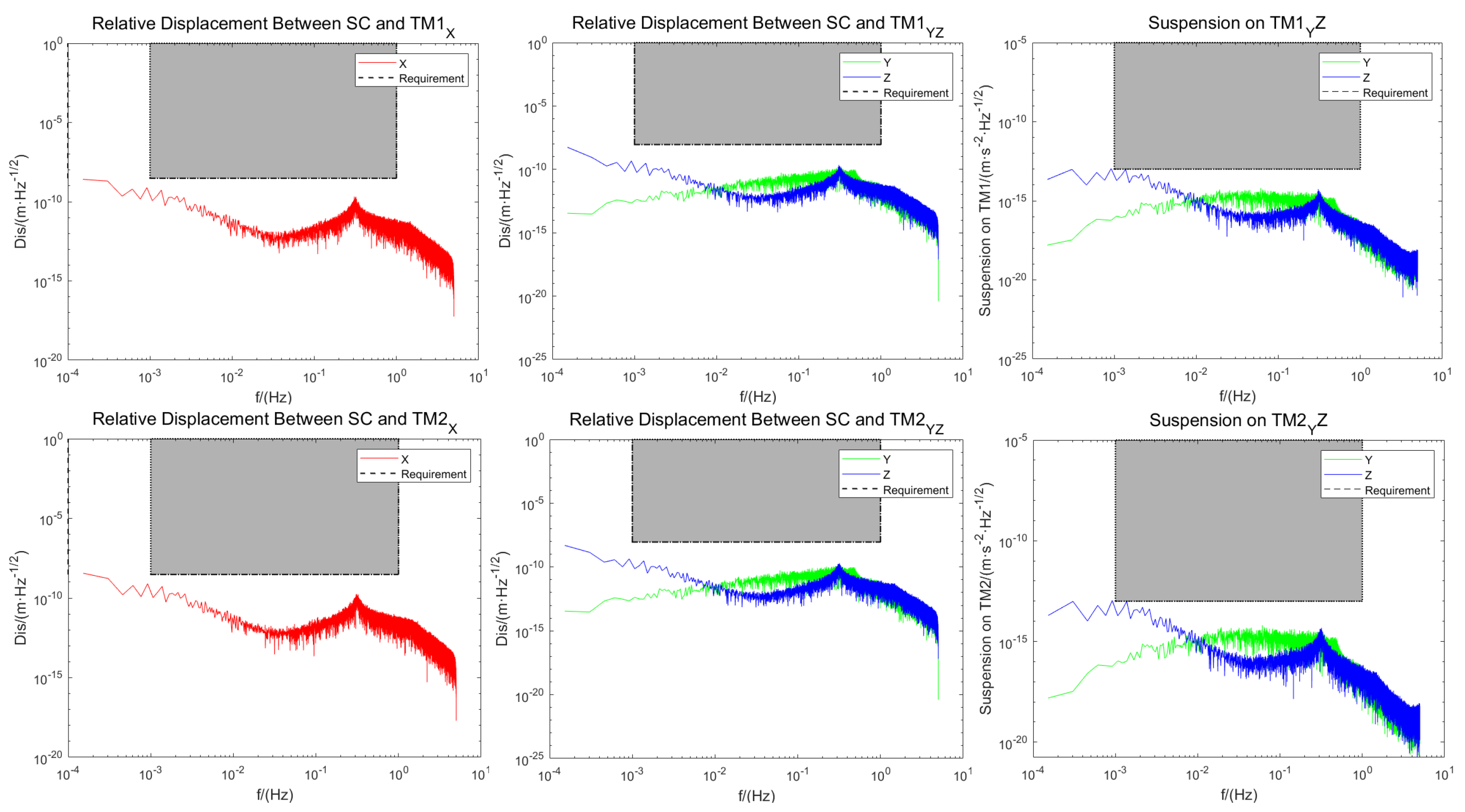
4.1. Requirements

In order to provide a feasible situation for the deep space detection, the residual acceleration on the test masses must be limited to $1\times {10}^{-15}$ m/(s²·Hz^1/2) along the sensitive axis. In this study, the residual acceleration index was classified into three categories: the nonconservative force on the test masses, the suspension control signal, and the stiffness force caused by the relative motion between the test mass and spacecraft.

For the control aspect of the system, it is crucial to focus on the relative jitter between the spacecraft and test masses, as well as the control signal resulting from the suspension control loop. The maximum signals are constrained according to

Table 1. Requirements for TianQin mission (1 mHz < f < 1 Hz).

Axis	Electrostatic Actuation Signal	Relative Jitter
X	–	$1\times {10}^{-9}$ m/Hz1/2
Y	$1\times {10}^{-13}$ m/(s2·Hz1/2)	$3\times$ 10−9 m/Hz1/2
Z	$1\times$ 10−13 m/(s2·Hz1/2)	$3\times {10}^{-9}$ m/Hz1/2

.

4.2. Boundary Conditions

The control processes for test masses were divided into two stages. First, the constraint of actuator saturation was applied to control the test masses in order to limit the initial release error of both test masses. During this stage, the requirements of the electrostatic actuation signal on the test masses specified in Table 1 could be disregarded, as there was no detection mission involved. Subsequently, in the next stage known as the drag-free science mode, a free-fall reference point was established for laser range finding. In this study, only the science mode stage was considered and its initial state was determined by the results obtained from the controlling mission during the first stage. And

Table 2. Initial state of test masses before science mode.

Axis	Initial Position Offset	Initial Derivative
$X_i$	$1\times {10}^{-7}$ m	$1\times {10}^{-9}$ m/s
$Y_i$	$1\times {10}^{-7}$ m	$1\times {10}^{-9}$ m/s
$Z_i$	$1\times {10}^{-7}$ m	$1\times {10}^{-9}$ m/s
${\phi }_i$	$0.1\times \pi /180$	$1\times {10}^{-8}$ rad/s
${\theta }_i$	$0.1\times \pi /180$	$1\times {10}^{-8}$ rad/s
${\psi }_i$	$0.1\times \pi /180$	$1\times {10}^{-8}$ rad/s

indicates the initial conditions.

• where $i=1,2$ represent TM1 and TM2, respectively.

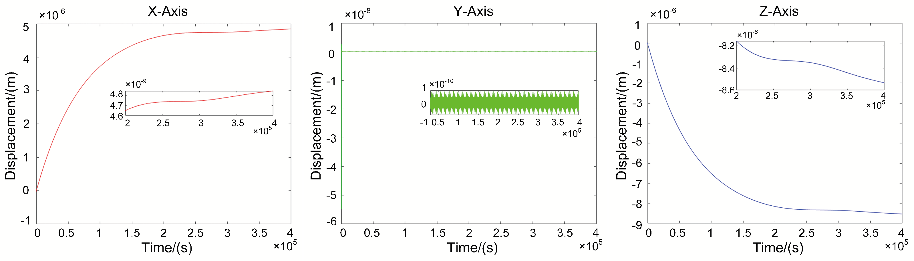
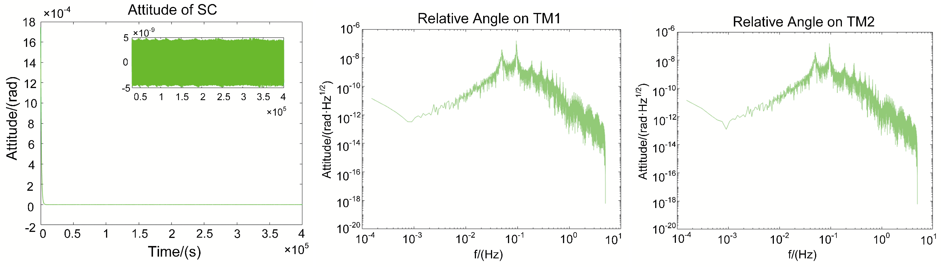
4.3. Simulations

The design of the DFAC system was verified with the simulation of the whole system, and the simulation was undertaken in Matlab/Simulink. A block diagram of the system simulation is shown in Figure 9.

The nonconservative forces and torques on the test masses in the simulation were generated by white noise, where the disturbing torque of the satellite in the simulation was set to a certain order of magnitude and the power spectral density (PSD) results were obtained based on a frequency of 10 Hz.

Frequency performance of the control strategy in this study is shown in Figure 10, including the PSD results of the offsets of TM1 and TM2 along all of the axes and PSD results of the control signal on test masses, which was limited by the requirements in Table 1, and the outputs of the micro-thrust system for the satellite and square of the voltage of the actuator on TM1 and TM2 are shown in Figure 11.

It is obvious that the trajectories of both TM1 and TM2 were convergent. We took TM1 as an example, and the results are shown in Figure 12.

The attitude controllers for the satellite and test masses were designed without mechanisms that rotate the load internally; thus, the design for this system provides a reference result for future work, and the result of the attitude control system was evaluated without requirements. We took the Y-axis as the example, where the attitude of the satellite and relative angle between the satellite and test masses are shown in Figure 13.

We conclude by stating that the drag-free and attitude control system with the optimization and assignment for the actuation system was designed for the science mode in this study; the dynamics were decoupled into three loops; the results showed that the requirements were met for the mission based on the assumptions; the relative displacement between each test mass and the center of the relevant cage was controlled to within a magnitude of ${10}^{-6}$ m; and the PSD results in the simulation showed that the suspension force was limited to ${10}^{-13}$ m/s²/Hz^1/2 along the insensitive axis for each test mass, where the complete simulation was undertaken in MATLAB and Simulink.

5. Conclusions

In this paper, we present a comprehensive analysis and design of a drag-free and attitude control system that was specifically applied to gravitational wave detection formation based on the background of the TianQin mission. By strategically allocating actuators and designing controllers, we successfully developed a scientific exploration spacecraft system that fulfills our requirements. This novel design holds great potential for widespread application in in-orbit drag-free formations dedicated to deep space exploration missions. Moreover, the flexibility of adjusting design parameters according to specific celestial bodies, such as the Sun or other potential orbits, further enhances the versatility of our proposed system. It is foreseeable that this technology will experience accelerated development and application in the future, particularly in the realms of conducting space scientific experiments and observing large-scale astronomical activities. However, it should be noted that the current design of this article lacks consideration for mass distribution and platform rotation requirements pertaining to other load components apart from the drag-free system, such as those employed for optical communication or celestial phenomena observation. These intricate aspects warrant further exploration and analysis in future research.

References

- Bolton, S.J.; Levin, S.M.; Guillot, T.; Li, C.; Kaspi, Y.; Orton, G.; Wong, M.H.; Oyafuso, F.; Allison, M.; Arballo, J.; et al. Microwave observations reveal the deep extent and structure of Jupiter’s atmospheric vortices. Science 2021, 374, 968–972. [Google Scholar] [CrossRef] [PubMed]
- Choi, S.-J.; Kang, H.; Lee, K.; Kwon, S. A Pattern Search Method to Optimize Mars Exploration Trajectories. Aerospace 2023, 10, 827. [Google Scholar] [CrossRef]
- Palos, M.F.; Janhunen, P.; Toivanen, P.; Tajmar, M.; Iakubivskyi, I.; Micciani, A.; Orsini, N.; Kütt, J.; Rohtsalu, A.; Dalbins, J.; et al. Electric Sail Mission Expeditor, ESME: Software Architecture and Initial ESTCube Lunar Cubesat E-Sail Experiment Design. Aerospace 2023, 10, 694. [Google Scholar] [CrossRef]
- Malgarini, A.; Franzese, V.; Topputo, F. Application of Pulsar-Based Navigation for Deep-Space CubeSats. Aerospace 2023, 10, 695. [Google Scholar] [CrossRef]
- Orosei, R.; Lauro, S.E.; Pettinelli, E.; Cicchetti, A.N.D.R.E.A.; Coradini, M.; Cosciotti, B.; Di Paolo, F.; Flamini, E.; Mattei, E.; Pajola, M.; et al. Radar evidence of subglacial liquid water on Mars. Science 2018, 361, 490–493. [Google Scholar] [CrossRef] [PubMed]
- Ho, G.C.; Krimigis, S.M.; Gold, R.E.; Baker, D.N.; Slavin, J.A.; Anderson, B.J.; Korth, H.; Starr, R.D.; Lawrence, D.J.; McNutt, R.L., Jr.; et al. MESSENGER Observations of Transient Bursts of Energetic Electrons in Mercury’s Magnetosphere. Science 2011, 333, 1865–1868. [Google Scholar] [CrossRef] [PubMed]
- Lange, B. The drag-free satellite. AIAA J. 1964, 2, 1590–1606. [Google Scholar] [CrossRef]
- Sereno, M.; Sesana, A.; Bleuler, A.; Volonteri, M.; Jetzer, P.; Begelman, M.C. Strong Lensing of Gravitational Waves as Seen by LISA. Phys. Rev. Lett. 2010, 105, 251101. [Google Scholar] [CrossRef] [PubMed]
- Toubiana, A.; Sberna, L.; Caputo, A.; Cusin, G.; Marsat, S.; Jani, K.; Babak, S.; Barausse, E.; Caprini, C.; Pani, P.; et al. Detectable Environmental Effects in GW190521-like Black-Hole Binaries with LISA. Phys. Rev. Lett. 2021, 126, 101105. [Google Scholar] [CrossRef]
- Badger, C.; Martinovic, K.; Torres-Forné, A.; Sakellariadou, M.; Font, J.A. Dictionary Learning: A Novel Approach to Detecting Binary Black Holes in the Presence of Galactic Noise with LISA. Phys. Rev. Lett. 2023, 130, 091401. [Google Scholar] [CrossRef]
- Huang, S.; Hu, Y.; Korol, V.; Li, P.C.; Liang, Z.C.; Lu, Y.; Wang, H.T.; Yu, S.; Mei, J. Science with the TianQin Observatory: Preliminary results on Galactic double white dwarf binaries. Phys. Rev. D 2020, 101, 103027. [Google Scholar] [CrossRef]
- Fan, H.; Hu, Y.; Barausse, E.; Sesana, A.; Zhang, J.D.; Zhang, X.; Zi, T.G.; Mei, J. Science with the TianQin Observatory: Preliminary result on extreme-mass-ratio inspirals. Phys. Rev. D 2020, 104, 064008. [Google Scholar]
- Wang, H.; Jiang, Z.; Sesana, A.; Barausse, E.; Huang, S.J.; Wang, Y.F.; Feng, W.F.; Wang, Y.; Hu, Y.M.; Mei, J.; et al. Science with the TianQin Observatory: Preliminary result on massive black hole binaries. Phys. Rev. D 2019, 101, 103027. [Google Scholar] [CrossRef]
- Liang, Z.; Hu, Y.; Jiang, Y.; Cheng, J.; Zhang, J.D.; Mei, J. Science with the TianQin Observatory: Preliminary results on stochastic gravitational-wave background. Phys. Rev. D 2022, 105, 022001. [Google Scholar] [CrossRef]
- Liu, S.; Zhu, L.; Hu, Y.; Zhang, J.D.; Ji, M.J. Capability for detection of GW190521-like binary black holes with TianQin. Phys. Rev. D 2022, 105, 023019. [Google Scholar] [CrossRef]
- Nobili, A.M.; Anselmi, A. Testing the equivalence principle in space after the MICROSCOPE mission. Phys. Rev. D 2018, 98, 042002. [Google Scholar] [CrossRef]
- Wang, G.; Han, W. Observing gravitational wave polarizations with the LISA-TAIJI network. Phys. Rev. D 2021, 103, 024012. [Google Scholar] [CrossRef]
- Wang, G.; Han, W. Alternative LISA-TAIJI networks: Detectability of the isotropic stochastic gravitational wave background. Phys. Rev. D 2021, 104, 104015. [Google Scholar] [CrossRef]
- Omiya, H.; Seto, N. Searching for anomalous polarization modes of the stochastic gravitational wave background with LISA and Taiji. Phys. Rev. D 2020, 102, 084053. [Google Scholar] [CrossRef]
- Van Patten, R.A.; Everitt, C.W.F. Possible Experiment with Two Counter-Orbiting Drag-Free Satellites to Obtain a New Test of Einstein’s General Theory of Relativity and Improved Measurements in Geodesy. Phys. Rev. Lett. 1976, 36, 629–632. [Google Scholar] [CrossRef]
- Armano, M.; Audley, H.; Baird, J.; Binetruy, P.; Born, M.; Bortoluzzi, D.; Castelli, E.; Cavalleri, A.; Cesarini, A.; Cruise, A.M.; et al. LISA Pathfinder Performance Confirmed in an Open-Loop Configuration: Results from the Free-Fall Actuation Mode. Phys. Rev. Lett. 2019, 123, 111101. [Google Scholar] [CrossRef] [PubMed]
- Touboul, P.; Métris, G.; Rodrigues, M.; Bergé, J.; Robert, A.; Baghi, Q.; André, Y.; Bedouet, J.; Boulanger, D.; Bremer, S.; et al. MICROSCOPE Mission: Final Results of the Test of the Equivalence Principle. Phys. Rev. Lett. 2022, 129, 121102. [Google Scholar] [CrossRef] [PubMed]
- Abich, K.; Abramovici, A.; Amparan, B.; Baatzsch, A.; Okihiro, B.B.; Barr, D.C.; Bize, M.P.; Bogan, C.; Braxmaier, C.; Burke, M.J.; et al. In-Orbit Performance of the GRACE Follow-on Laser Ranging Interferometer. Phys. Rev. Lett. 2019, 123, 031101. [Google Scholar] [CrossRef] [PubMed]
- Drinkwater, M.R.; Floberghagen, R.; Haagmans, R.; Muzi, D.; Popescu, A. GOCE: ESA’s First Earth Explorer Core Mission. Space Sci. Rev. 2003, 108, 419–432. [Google Scholar] [CrossRef]
- Kremer, K.; Chatterjee, S.; Breivik, K.; Rodriguez, C.L.; Larson, S.L.; Rasio, F.A. LISA Sources in Milky Way Globular Clusters. Phys. Rev. Lett. 2018, 120, 191103. [Google Scholar] [CrossRef] [PubMed]
- Schumaker, B. Disturbance reduction requirements for LISA. Class. Quantum Gravity 2003, 20, S239–S253. [Google Scholar] [CrossRef]
- Luo, J.; Chen, L.S.; Duan, H.Z.; Gong, Y.G.; Hu, S.; Ji, J.; Liu, Q.; Mei, J.; Milyukov, V.; Sazhin, M.; et al. TianQin: A space-borne gravitational wave detector. Class. Quantum Gravity 2016, 33, 035010. [Google Scholar] [CrossRef]
- Hu, X.C.; Li, X.H.; Wang, Y.; Feng, W.F.; Zhou, M.Y.; Hu, Y.M.; Hu, S.C.; Mei, J.W.; Shao, C.G. Fundamentals of the orbit and response for TianQin. Class. Quantum Gravity 2018, 35, 095008. [Google Scholar] [CrossRef]
- Gerardi, D.; Allen, G.; Conklin, J.W.; Sun, K.X.; DeBra, D.; Buchman, S.; Gath, P.; Fichter, W.; Byer, R.L.; Johann, U.; et al. Advanced drag-free concepts for future space-based interferometers: Acceleration noise performance. Rev. Sci. Instrum. 2014, 85, 1590–1606. [Google Scholar] [CrossRef]
- Liu, H.; Luo, Z.; Jin, G. The development of phasemeter for Taiji space gravitational wave detection. Microgravity Sci. Technol. 2018, 30, 775–781. [Google Scholar] [CrossRef]
- Ye, B.B.; Zhang, X.; Zhou, M.Y.; Wang, Y.; Yuan, H.M.; Gu, D.; Ding, Y.; Zhang, J.; Mei, J.; Luo, J. Optimizing orbits for TianQin. Int. J. Mod. Phys. D 2019, 9, 1950121. [Google Scholar] [CrossRef]
- Canuto, E.S. Drag-free and attitude control for the GOCE satellite. Automatica 2008, 44, 1766–1780. [Google Scholar] [CrossRef]
- Zhang, C.; He, J.; Duan, L.; Kang, Q. Design of an Active Disturbance Rejection Control for Drag-Free Satellite. Microgravity Sci. Technol. 2019, 31, 31–48. [Google Scholar] [CrossRef]
- Delavault, S.; Prieur, P.; Liénart, T.; Robert, A.; Guidotti, P.Y. MICROSCOPE mission: Drag-free and attitude control system expertise activities toward the scientific team. CEAS Space J. 2018, 10, 487–500. [Google Scholar] [CrossRef]
- Liao, H.; Xu, Y.; Zhu, Z.; Deng, Y.; Zhao, Y. A new design of drag-free and attitude control based on non-contact satellite. ISA Trans. 2019, 88, 62–72. [Google Scholar] [CrossRef] [PubMed]
- Canuto, E.; Massotti, L.; Molano-Jimenez, A.; Perez, C.N. Drag-free and attitude control for long-distance, low-Earth-orbit, gravimetric satellite formation. In Proceedings of the 29th Chinese Control Conference, Beijing, China, 29–31 July 2011. [Google Scholar]
- Dang, Z.; Zhang, Y. Relative position and attitude estimation for inner-formation gravity measurement satellite system. Acta Astronaut 2011, 69, 514–525. [Google Scholar] [CrossRef]
- Ji, L.; Liu, K.; Xiang, J. On all-propulsion design of integrated orbit and attitude control for inner-formation gravity field measurement satellite. Sci. China Technol. Sci. 2011, 54, 3233–3242. [Google Scholar] [CrossRef]
- Grynagier, A.; Ziegler, T.; Fichter, W. Identification of dynamic parameters for a one-axis drag-free gradiometer. IEEE Trans. Aerosp. Electron. Syst. 2013, 49, 341–355. [Google Scholar] [CrossRef]
- Xiao, C.; Bai, Y.; Li, H.; Liu, L.; Liu, Y.; Luo, J.; Ma, Y.; Qu, S.; Tan, D.; Wang, C.; et al. Drag-free control design and in-orbit validation of TianQin-1 satellite. Class. Quantum Gravity 2022, 39, 155001. [Google Scholar] [CrossRef]
- Gath, P.; Fichter, W.; Kersten, M.; Schleicher, A. Drag free and attitude control system design for the LISA Pathfinder mission. In Proceedings of the AIAA Guidance, Navigation, and Control Conference and Exhibit, Providence, RI, USA, 16–19 August 2004. [Google Scholar]
- Wu, S.F.; Fertin, D. Spacecraft drag-free attitude control system design with quantitative feedback theory. Acta Astronaut. 2008, 62, 668–682. [Google Scholar] [CrossRef]
- Gath, P.F.; Schulte, H.R. Drag free and attitude control system design for the LISA science mode. In Proceedings of the AIAA Guidance, Navigation, and Control Conference and Exhibit, Hilton Head, SC, USA, 20–23 August 2007. [Google Scholar]
- Sun, X.; Shen, Q.; Wu, S. Partial State Feedback MRAC-Based Reconfigurable Fault-Tolerant Control of Drag-Free Satellite With Bounded Estimation Error. IEEE Trans. Aerosp. Electron. Syst. 2023, 59, 6570–6586. [Google Scholar] [CrossRef]
- Sun, X.; Shen, Q.; Wu, S. Event-triggered robust model reference adaptive control for drag-free satellite. Adv. Space Res. 2023, 72, 4984–4996. [Google Scholar] [CrossRef]
- Lian, X.; Zhang, X.; Lu, L.; Wang, J.; Liu, L.; Sun, J.; Sun, Y. Frequency Separation Control for Drag-Free Satellite With Frequency-Domain Constraints. IEEE Trans. Aerosp. Electron. Syst. 2021, 57, 4085–4096. [Google Scholar] [CrossRef]
- Hao, L.; Zhang, Y. Extended observer and output feedback control for the preliminary design of tianqin two-test-mass drag-free and attitude control system. In Proceedings of the International Astronautical Congress, Virtual, Online, 12–14 October 2020. [Google Scholar]
- Buffington, J.M.; Kapila, V.; Sparks, A.G. Spacecraft formation flying: Dynamics and control. J. Guid. Control Dyn. 1999, 6, 4137–4141. [Google Scholar]
- Ziegler, T.; Fichter, W. Test mass stiffness estimation for the LISA Pathfinder drag-free system. In Proceedings of the AIAA Guidance, Navigation, and Control Conference and Exhibit, Hilton Head, SC, USA, 20–23 August 2007. [Google Scholar]
- Fichter, W.; Schleicher, A.; Bennani, S.; Wu, S. Closed loop performance and limitations of the LISA pathfinder drag-free control system. In Proceedings of the AIAA Guidance, Navigation, and Control Conference and Exhibit, Hilton Head, SC, USA, 20–23 August 2007. [Google Scholar]
- Antonucci, F.; Armano, M.; Audley, H.; Auger, G.; Benedetti, M.; Binetruy, P.; Boatella, C.; Bogenstahl, J.; Bortoluzzi, D.; Bosetti, P.; et al. LISA Pathfinder: Mission and status. Class. Quantum Gravity 2011, 28, 094001. [Google Scholar] [CrossRef]
- Weber, W.J.; Bortoluzzi, D.; Cavalleri, A.; Carbone, L.; Da Lio, M.; Dolesi, R.; Fontana, G.; Hoyle, C.D.; Hueller, M.; Vitale, S. Position sensors for flight testing of LISA drag-free control. In Proceedings of the Astronomical Telescopes and Instrumentation, Waikoloa, HI, USA, 26 February 2003. [Google Scholar]
- Han, J.Q. From PID to Active Disturbance Rejection Control. IEEE Trans. Ind. Electron. 2009, 56, 900–906. [Google Scholar] [CrossRef]
- Gao, Z.Q. Scaling and bandwidth-parameterization based controller tuning. In Proceedings of the 2003 American Control Conference, Denver, CO, USA, 4–6 June 2003. [Google Scholar]