Towards Global Explainability of Artificial Intelligence Agent Tactics in Close Air Combat

Abstract

In this paper, we explore the development of an explainability system for air combat agents trained with reinforcement learning, thus addressing a crucial need in the dynamic and complex realm of air combat. The safety-critical nature of air combat demands not only improved performance but also a deep understanding of artificial intelligence (AI) decision-making processes. Although AI has been applied significantly to air combat, a gap remains in comprehensively explaining an AI agent’s decisions, which is essential for their effective integration and for fostering trust in their actions. Our research involves the creation of an explainability system tailored for agents trained in an air combat environment. Using reinforcement learning, combined with a reward decomposition approach, the system clarifies the agent’s decision making in various tactical situations. This transparency allows for a nuanced understanding of the agent’s behavior, thereby uncovering their strategic preferences and operational patterns. The findings reveal that our system effectively identifies the strengths and weaknesses of an agent’s tactics in different air combat scenarios. This knowledge is essential for debugging and refining the agent’s performance and to ensure that AI agents operate optimally within their intended contexts. The insights gained from our study highlight the crucial role of explainability in improving the integration of AI technologies within air combat systems, thus facilitating more informed tactical decisions and potential advancements in air combat strategies.

1. Introduction

In recent years, the application of Artificial Intelligence (AI)-driven Autonomous Systems (ASs) in real-world scenarios has seen a remarkable surge, thus demonstrating highly complex and novel behaviors. This expansion includes diverse domains, such as large air combat vehicles [1] and smaller autonomous Remotely Piloted Aircraft Systems (RPASs) [2], which employ AI to improve operational autonomy and effectiveness. However, these advances have highlighted the critical need for explainability in these autonomous systems [3]. The importance of explainability extends beyond mere user comprehension and encompasses the building of trust among users, developers, and policymakers alike. Furthermore, in the context of safety-critical applications, such as autonomous air combat agents, the role of explainability is of even greater significance. As given in [4,5], explainability serves as one of the pillars of trustworthiness of AI-driven ASs along with verification, certification, and adaptability, especially in high-stakes safety critical environments. The role of explainability is to present users with the rationale behind AI actions to enable them to build higher-quality mental models. Formally, mental models are “internal representations that people build based on their experiences in the real world” [6]. Explainability allows users to construct higher-quality mental models by offering insights into the rationale behind AI actions, thus resulting in more effective human–AI collaboration. Although explainable AI methods have made significant progress in various domains such as healthcare, the judiciary, and finance [7], the application of these methods to AI-driven air combat agents remains relatively unexplored. In air combat environments, pilots are tasked with making high-frequency sequential decisions within highly dynamic and challenging environments. Explainability enables better integration of AI into air combat by assisting in the discovery and refinement of new tactics, as well as improves overall trust in AI applications.

The main aim of this work is to address the critical need for explainability in AI-driven Autonomous Systems (ASs), especially in high-stakes safety-critical environments such as air combat. This research is grounded in the understanding that while AI has significantly improved operational capabilities in various domains, its integration in complex scenarios such as air combat is hindered by a lack of explainability and transparency in its decision making. The overarching goal is to enhance trust and effective human–AI collaboration by developing methods that make AI actions understandable and reliable. By focusing on this aspect, this work aims to contribute to the broader field of trustworthy AI, which is a key concern in the current era of rapidly advancing autonomous technologies.

With the ever-increasing advancement of AI, the need for a trustworthy and transparent AI system becomes more evident. Explainable Artificial Intelligence (XAI) has emerged as a pivotal field, thus trying to address the need for transparency and understandability gap in AI decision-making processes. A branch of these AI systems employing the Deep Learning (DL) method uses a multilayer neural network (NN) at its core to solve some of the most complex problems ranging from classification to autonomous driving. The lack of transparency comes from the use of these deep NNs and their inherent black box-like nature. Some methods have been developed to address these issues such as [8], where they introduced a method called LIME that provides a local explanation of why an AI system made certain classification predictions. The explanation shows how much each feature contributed to the resultant classification, thus providing insight to the user about the AI system preferences. Similar to the LIME method, [9] introduced SHAPLEY, which uses Shapley values to identify how individual feature contribute to the model’s output. Some advancement has also been made in explaining vision-based AI systems like the saliency map [10] and GradCAM [11].

The recent success of DL methods has also benefited a branch of AI called Reinforcement Learning (RL). Deep RL methods have shown great success in multiple applications ranging from playing Atari and board games [12,13] to complex real-world robotics applications, including hand manipulation [14], aerial acrobatic drone flight [15], and champion level drone racing [16].

The generation of air combat tactics using RL has been studied extensively in the literature. An air combat tactic is a specific maneuver or action executed by a pilot to gain an advantage over an opponent during an immediate engagement. A notable study by [17] explored the use of the deep deterministic policy gradient (DDPG) for training RL agents, thus resulting in considerable performance enhancements in within-visual-range (WVR) combat. Another work by [18] delved into multiagent reinforcement learning (MARL) to model intricate, cooperative air combat strategies involving several aircraft, thus showcasing the potential of RL in complex scenarios. Ref. [19] employed hierarchical reinforcement learning (HRL) to decompose combat missions into manageable subtasks, thus streamlining training and decision-making processes. Ref. [20] investigated the efficacy of model-based RL in accelerating convergence and improving sample efficiency during air combat agent training, thereby contributing to better performance in dynamic environments. Lastly, ref. [21] applied advanced deep reinforcement techniques called Proximal Policy Optimization (PPO) and Soft Actor–Critic (SAC) and compared their performance. The development of air combat agents using deep RL methods was also explored during the DARPA AlphaDogFight trial [1].

Despite their great success, deep RL methods also suffer from a lack of explainability due to the black box nature of NNs. Explaining the rationale behind these RL agents’ actions has recently gained interest. However, the field still has not matured enough to have a concise definition and categorization of different explanation types. Multiple surveys use different methods to categorize Explainable RL (XRL) methods [22,23,24]. These categorizations can be briefly divided into the scope and source of explanation. The scope consists of global vs. local explainability, and the source consists of intrinsic vs. extrinsic explainability. There are also policy simplification methods, where deep NN is simplified to decision trees or linear regression models [25,26]. However, policy simplification approaches compromise performance to create an explainable model. When the depth of the tree is increased to match the performance, it grows large enough to negate its advantage in explainability. The local explanation explains the agent’s current action for a given state, whereas the global method gives an explanation for more broader states. An intrinsic explanation is defined as an explanation coming from the model itself, like a decision tree, whereas extrinsic methods provide an explanation outside the model.

Causal explanation approaches have been proposed to address “what if” questions, thus offering insights into the relationships between actions and resulting states or events. However, these methods depend on understanding the causal model that links specific actions with their consequences [27]. Research into discovering causal structures in continuous-state games has been studied, yet this approach requires an understanding of the environment’s model within the explanation method itself, with example explanations revealing relationships within the game’s differential equations [28]. Applying causal explanations within the air combat context presents particular challenges due to the high-dimensional and dynamic nature of the state space, as well as the complexity arising from the interactions among multiple agents, with each guided by distinct policies.

In [29], the authors proposed the notion of the intended outcome, where the belief map is trained along with the Q function for explanation purposes. Although a mathematical proof was given for why the belief map is a true representation of the Q function used in decision making, the paper lacks reasons as to why this is different from directly simulating the Q function and how it provides an explanation into an agent’s decision making. This approach is also limited to the tabular environment, thus making it unsuitable for the continuous dynamics of air combat environments.

The HIGHLIGHTS method has been proposed to summarize an agent’s behavior to assist individuals in assessing the capabilities of these agents [30]. The summary explanation is derived by calculating the state importance value, which represents the difference between the highest and lowest Q values from multiple simulation runs at each state, with the aim of offering a global explanation through concise clips of the most crucial states. This approach has been applied to saliency maps [31] and reward decomposition [32], with a user study having been conducted to investigate its effectiveness. In [32], the authors highlight the effectiveness of reward decomposition in conveying the agent’s preferences and note the limited contribution of the HIGHLIGHTS method. It is also mentioned that discerning reward decomposition becomes more challenging when observing dynamic videos instead of static images [31,32]. Although state-based global policy summarization approaches provide some insight into agent behavior, the explanations provided are constrained by the limited number of unique states visited during randomly initialized simulation runs. Furthermore, these explanations are anecdotal and therefore cannot be considered representative of the agent’s overall policy.

The concept of the influence predictor has been defined in [33], where a separate network is trained for each reward type using the absolute value of the reward value. A human evaluation study reveals that participants found the influence predictor significantly useful compared to the Q value that was provided for each state. The paper also concludes that although the proposed method increased the understanding of the participants, none of the investigated explanation methods had a high trust score.

The reward decomposition approach has been proposed to provide an explanation in an agent’s decision-making process by breaking down the scalar reward value into semantically meaningful reward types, thus allowing analysis of the contribution of each reward type to the chosen action in a given state [34,35]. Reward decomposition has proven to be effective in improving the understanding and trust of non-AI experts in scenarios with discrete states and action spaces, particularly in simple board games [36]. However, these applications have been predominantly demonstrated in simple games. Human evaluation studies conducted in [32,33,36] showed that presenting the agent’s expectation in terms of decomposed reward allowed users to have a better mental model and to make a better assessment of the agent’s preference. They also conclude that there is no one-size-fits-all explanation approach, and it is environment and task dependent.

The main aim of this work is to develop an explainability framework specifically designed for AI agents involved in air combat trained with reinforcement learning. This system is intended to demystify the decision-making processes of AI agents, thus revealing their preferences and operational patterns in various tactical situations. By doing so, the research seeks to identify the strengths and weaknesses of AI tactics in air combat, thereby enabling more effective debugging and performance optimization. The ultimate objective is to ensure that AI agents not only perform optimally but also operate in a manner that is explainable and understandable to human operators, thereby bridging the gap between advanced AI capabilities and their practical, real-world applications in air combat environments.

Our contributions to Explainable Reinforcement Learning (XRL) research are marked by several key advances. First, we extend local explanations to global explanations using tactical regions, thus offering a broader view of an agent’s decision-making process across different combat scenarios. Second, we introduce a visual explanation approach for reward decomposition, thus providing an innovative means to visually interpret an agent’s decision-making process. Third, by applying our approach to the air combat environment, we demonstrate its effectiveness in identifying dominant reward types and their relative contributions across tactical regions, thus uncovering insights into an agent’s decision-making process. Our global explanation approach, grounded in the context of tactical regions, enables a deeper understanding of the agent’s priorities and decision-making rationale. The visual explanation method further enhances this understanding by making complex patterns of preference easily accessible and explainable. Through the application of these methods in the air combat domain, we showcase the applicability of our approaches by highlighting potential areas for refinement and alignment with human expectations. This collective body of work significantly advances the field of XRL by providing powerful tools for explaining, debugging, and refining AI agents in complex dynamic environments.

The rest of the paper is organized as follows. Section 2 provides background information detailing the air combat environment, including its state space, action space, and reward function, along with an overview of the Deep Q Network (DQN), reward decomposition methods, and training details. Section 3 goes into explainability by elaborating on local explanation, global explanation within tactical regions, the application of global explanation to the air combat environment, and the method of global visual explanation. Finally, the discussion is given in Section 4, and the conclusion of this paper is given in Section 5.

2. Methodology

Incorporating explainability into a domain as complex as air combat requires a comprehensive understanding of the subject matter. This necessitates a systems engineering perspective focused on three key areas: first, crafting a reward function that is semantically meaningful, thus ensuring that it reflects objectives that are intuitively understood by humans; second, constructing a state space that approximates the sensory capabilities of pilots, thus facilitating a naturalistic representation of the environment that pilots would recognize; and third, streamlining the action space to alleviate computational burdens, thereby enabling decisions that are not only efficient but also cognitively plausible. This comprehensive strategy aims to bridge the gap between AI decision-making processes and human understanding, thus enhancing the system’s usability and effectiveness in real-world air combat scenarios.

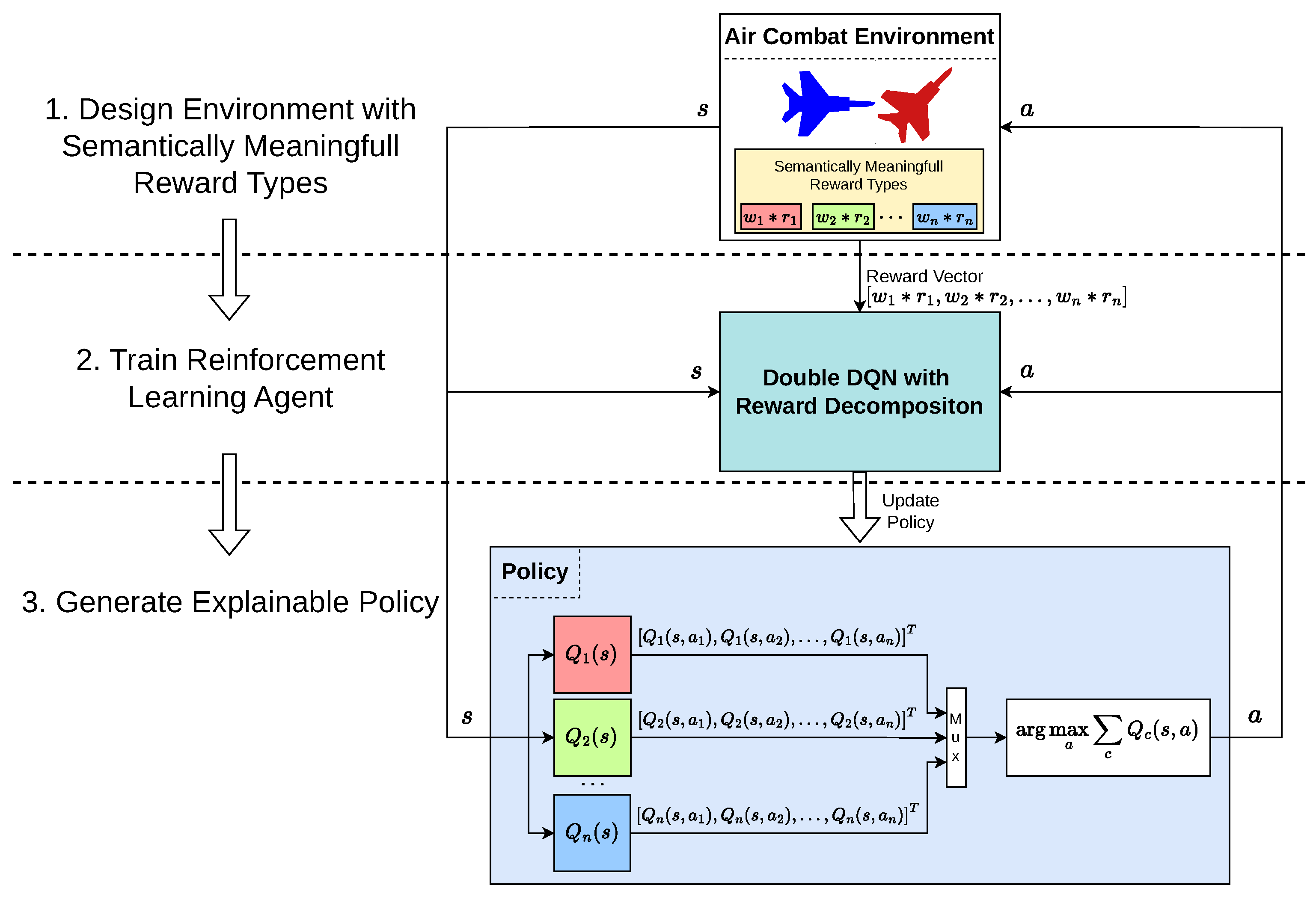
In this section, we present the comprehensive methodology used to develop and validate our framework to explain the decision-making process of the reinforcement learning (RL) agent in air combat simulations. We first start by looking back at our previous research, which inspired us to work on creating an explainable RL agent for air combat. Expanding on the acquired knowledge, we define the air combat simulation environment that enables the training and assessment of AI agents. This includes a comprehensive explanation of the state space, action space, and a reward function designed specifically to promote explainability within the system. We give details about the Deep Q Network (DQN) training algorithm to enable agents to learn the optimal policy by interacting with its environment. Additionally, we incorporate the concept of reward decomposition into the DQN algorithm to explain the agent’s decision-making process and provide a better understanding of its preference. We also provide training details, including parameter settings, environmental conditions, and reference open source libraries used for reproducibility purposes. The flow chart shown in Figure 1 represents the methodology followed in this study, thereby illustrating the sequential steps and connections between the different phases of developing an explainable reinforcement learning agent for air combat. The following visual representation provides a high-level overview of the steps taken.

2.1. Background

The quest for autonomy in air combat has led to significant advances in the application of artificial intelligence (AI), specifically through reinforcement learning (RL) to train agents capable of performing complex maneuvers. Historically, the control of agile maneuvering aircraft has posed a considerable challenge due to the dynamic and nonlinear nature of aerial combat environments. Numerous investigations have been conducted to devise tactics for resolving dogfight engagement issues since the mid-1900s [37]. Some studies have suggested rule-based techniques, also known as knowledge-encoded methods, in which experts used their experience to generate specific counter maneuvers appropriate for different scenarios [38]. The system utilizes a rule-based approach to choose a maneuver from a pre-established list, which is also referred to as the Basic Flight Maneuver (BFM). This selection is made by considering encoded expert conditional statements. A landmark study [39] demonstrated that the precise control of such maneuvers could be effectively achieved through modern control theory, thus employing a nested Nonlinear Dynamic Inversion (NDI) and Higher-Order Sliding Mode (HOSM) technique. This revelation laid the groundwork for using simplified versions of basic flight maneuvers, represented as discrete actions, to achieve control over aircraft movements within the simulation environment in this study.

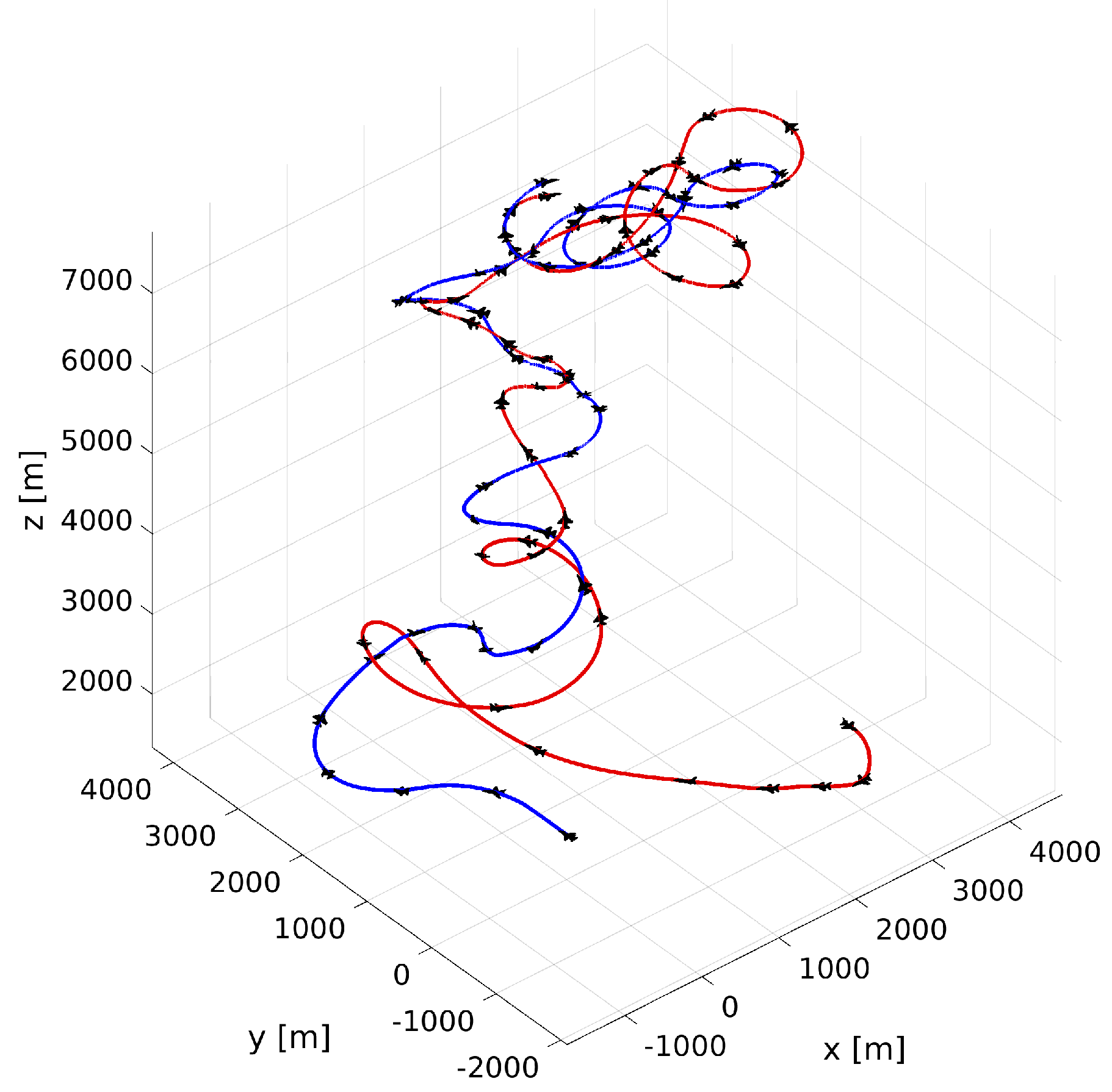
Expanding on these foundational insights, our research delved into the creation of a sophisticated 3D environment with the aim of training RL agents to excel in these maneuvers. The intricate dynamics of flight, combined with the complexity of aerial combat, require a platform where agents can learn and optimize their strategies in a controlled but realistic setting. By developing this 3D training environment, we were able to generate trajectory graphs, as depicted in Figure 2, which demonstrate the agents’ ability to navigate and execute combat tactics effectively. 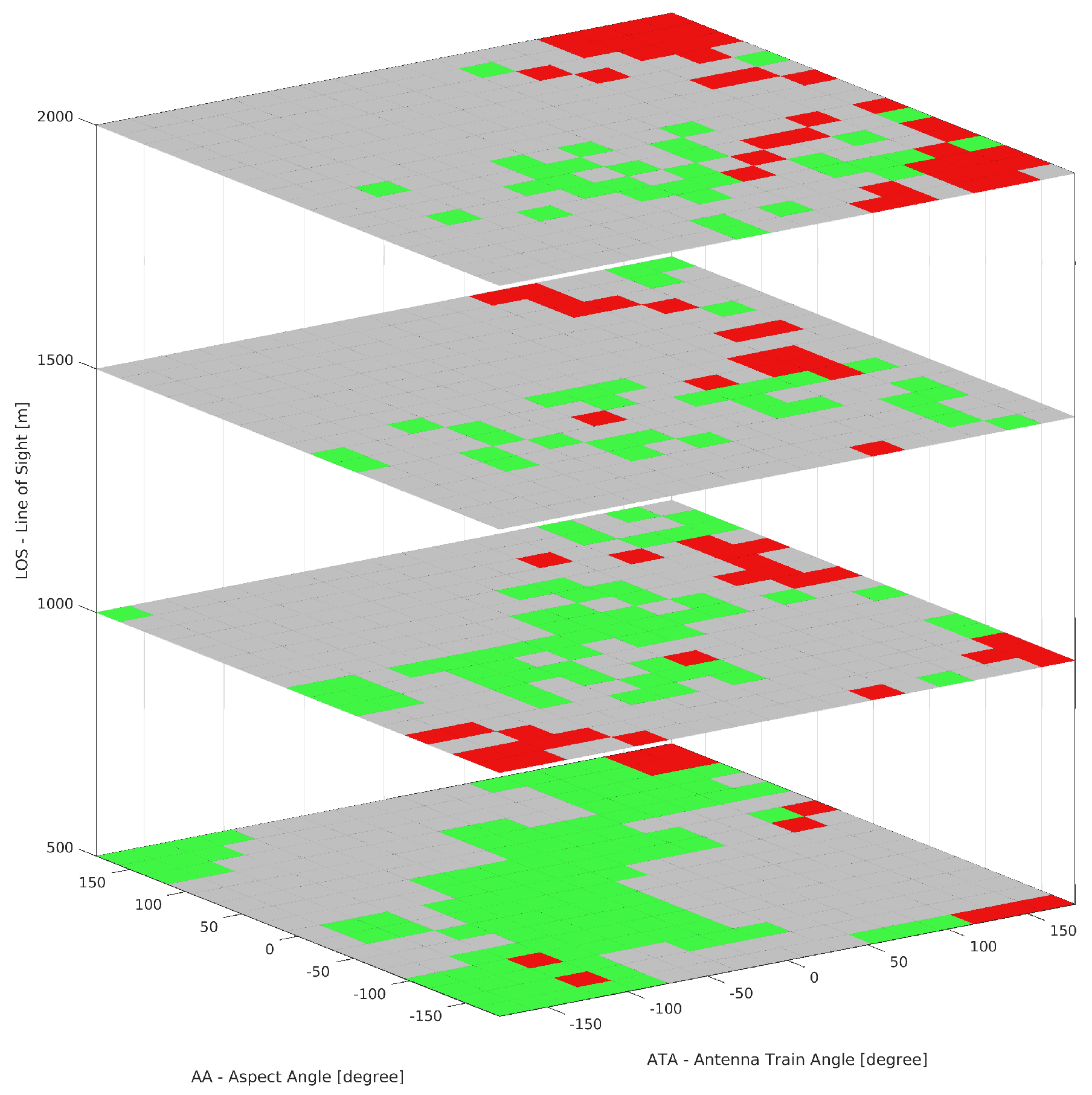However, our previous work [40] revealed inconsistencies in the performance of the RL agent. Despite starting from a symmetrical initial condition, when pitted against itself, our agent exhibited inconsistent superiority in different air combat regions, as illustrated in Figure 3. These findings motivated us to explore the incorporation of explainability into the decision-making process of these RL agents.

To address the critical challenge of explainability within this AI-driven air combat tactic generation problem, we recognized the need to simplify the operational environment from 3D to 2D. This strategic reduction not only streamlines the computational demands but, more importantly, enhances the clarity and interpretability of the agent’s decision-making processes. By focusing on a 2D environment using a smaller discrete action set, we aim to demystify the underlying strategies and logic employed by the AI in air combat scenarios. This paper will delve into the methodology and implications of introducing an explainability framework within this simplified 2D context, thus offering insights into the agent’s tactical reasoning and providing a transparent overview of its operational logic in different air combat tactical regions.

2.2. Air Combat Environment

This section presents information on a subpart of the air combat environment. This subpart includes a simplified mathematical model of the aircraft to decrease computation. In addition, it covers the selection of the state space, action space, and reward function to facilitate explainability in air combat agent.

The mathematical model of the aircraft used in an air combat environment is represented by a reduced order 3DOF aircraft dynamic [41] with the addition of variable speed, which is expressed as follows

$$\begin{array}{cc}\hfill \dot{V_c}& =\mathsf{\Delta }{V}_c\hfill \end{array}$$

(1)

$$\begin{array}{cc}\hfill \dot{{\chi }_c}& =\mathsf{\Delta }{\chi }_c\hfill \end{array}$$

(2)

$$\begin{array}{cc}\hfill \dot{V}& =K_V(V_c-V)\hfill \end{array}$$

(3)

$$\begin{array}{cc}\hfill \dot{\chi }& =K_{\chi }({\chi }_c-\chi )\hfill \end{array}$$

(4)

$$\begin{array}{cc}\hfill \dot{x}& =Vcos\left(\chi \right)\hfill \end{array}$$

(5)

$$\begin{array}{cc}\hfill \dot{y}& =Vsin\left(\chi \right)\hfill \end{array}$$

(6)

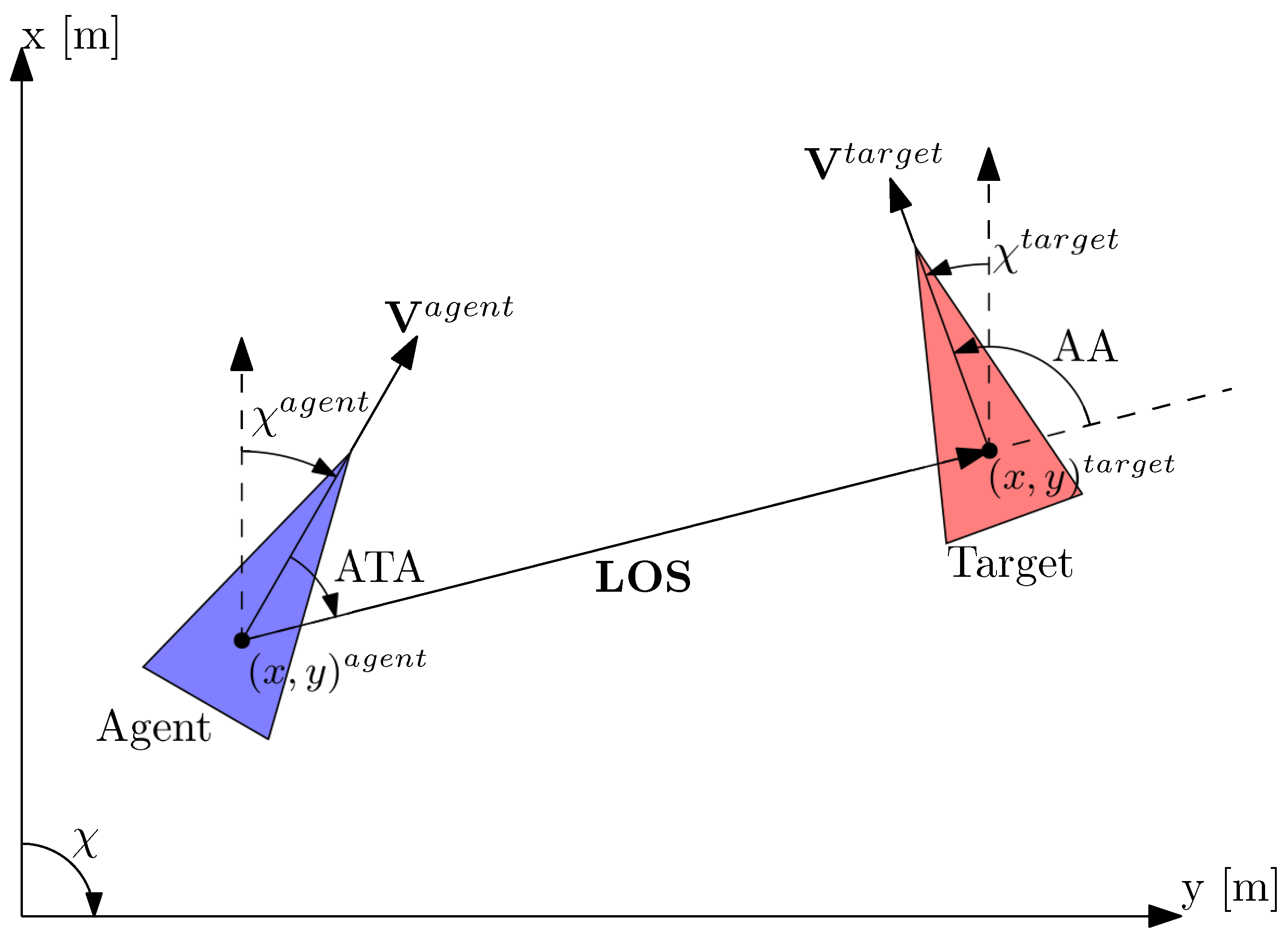
where $\mathsf{\Delta }{V}_c$ and $\mathsf{\Delta }{\chi }_c$ are the commanded delta speed and heading angle. $K_V$ and $K_{\chi }$ are the speed and heading angle gains. V and $\chi$ are the speed and heading angle states, respectively. The x and y represent the position state in the inertial frame. The geometric representations of these variables are shown in Figure 4. We used aerospace notation to represent coordinate frames, where X points towards up and Y points towards right. Following the right-hand rule, $\chi$ starts from the X axis as 0 and increases in the clockwise direction. The superscripts $agent$ and $target$ above $\mathbf{V}$ represent the own aircraft and the target aircraft’s velocity vector in m/s, respectively. $\mathbf{LOS}$ represents Line of Sight vector and it is defined from own aircraft’s center of mass ${(x,y)}^{agent}$ to the target aircraft’s center of mass ${(x,y)}^{target}$ in meters. The variables $ATA$ and $AA$ are defined in the following section. The advanced control technique discussed in [39] allows for finer control of the aircraft, thus allowing this simplified model to represent a wide range of maneuvers. Complex air combat maneuvers can be constructed by adjusting the control input $\mathsf{\Delta }{V}_c$ and $\mathsf{\Delta }{\chi }_c$. The limit and value of the model parameters used to simulate realistic aircraft are provided in the training details section.

2.2.1. State Space

Different state spaces have been used in the literature for the training of RL agents. In the DARPA competition, in addition to the relative position and angle between the aircraft, the angular speed of the enemy aircraft is also known [19]. In [21], they used the same state space but excluded Euler angle information for the target aircraft. In this paper, similar to our previous work [40,42], we used a smaller state space to replicate the limited perceptual capabilities of human pilots, thus creating a more realistic and relatable environment for explainability. The state space includes only relative measurements and does not contain information specific to the target aircraft.

Before we define state space, we introduce angles and other measurements commonly used in air combat environment. The geometric representation of the LOS vector, the ATA angle, the AA angle, and the velocity vectors is shown in Figure 4.

The Line of Sight (LOS) vector is defined from the center of mass of the agent aircraft ${(x,y)}^{agent}$ to the target aircraft’s center of mass ${(x,y)}^{target}$. This measurement conveys how far the target is from the agent aircraft. The LOS vector in the inertial frame is rotated to the local body frame of the agent aircraft, where the x axis is aligned with the agent velocity vector as follows:

$$\begin{array}{cc}\hfill d_x& =LO{S}_{x}sin\left({\chi }^{agent}\right)+LO{S}_{y}cos\left({\chi }^{agent}\right)\hfill \end{array}$$

(7)

$$\begin{array}{cc}\hfill d_y& =LO{S}_{x}cos\left({\chi }^{agent}\right)-LO{S}_{y}sin\left({\chi }^{agent}\right)\hfill \end{array}$$

(8)

$$\begin{array}{cc}\hfill LOS& =\sqrt{{LO{S}_x}^2+{LO{S}_y}^2}\hfill \end{array}$$

(9)

where ${\chi }^{agent}$ is the heading angle of the agent, $(LO{S}_x,LO{S}_y)$ is the component of the $\mathbf{LOS}$ vector in the inertial frame, $(d_x,d_y)$ is the component of the LOS vector defined in the local frame of the agent aircraft, and $LOS$ is magnitude of this $\mathbf{LOS}$ vector.

The Antenna Train Angle (ATA) is defined as the angle starting from the velocity vector of the agent aircraft ${\mathbf{V}}^{agent}$ to the LOS vector $\mathbf{LOS}$, and it increases clockwise. This gives a measurement of how much we are pointing towards the target aircraft. A value of $0^{\circ }$ indicates that the agent aircraft is pointing directly towards the target aircraft, while a value of ${180}^{\circ }$ indicates that it is pointing in the opposite direction of the target aircraft. The ATA angle is formulated as

$$ATA=arctan2\left(\frac{{\mathbf{V}}^{agent}\times \mathbf{LOS}}{{\mathbf{V}}^{agent}·\mathbf{LOS}}\right)$$

(10)

where ${\mathbf{V}}^{agent}$ and $\mathbf{LOS}$ represent the agent velocity vector and the LOS vector, respectively.

The Aspect Angle (AA) is defined as the angle starting from the LOS vector $\mathbf{LOS}$ to the target aircraft velocity vector ${\mathbf{V}}^{target}$, and it increases clockwise. It gives us a measurement of how much the target aircraft is pointing towards us. A value of $0^{\circ }$ indicates that the target is pointing in the opposite direction of the agent aircraft, whereas a value of ${180}^{\circ }$ indicates that it is pointing directly towards the agent aircraft. The AA angle is formulated as

$$AA=arctan2\left(\frac{\mathbf{LOS}\times {\mathbf{V}}^{target}}{\mathbf{LOS}·{\mathbf{V}}^{target}}\right)$$

(11)

where ${\mathbf{V}}^{target}$ represents the target velocity vector.

Lastly, the relative heading angle is defined as the angle that starts from the agent velocity vector to the target velocity vector. It gives us a measurement of the relative velocity direction of each aircraft. The relative heading angle is formulated as

$${\chi }_{rel}=arctan2\left(\frac{{\mathbf{V}}^{agent}\times {\mathbf{V}}^{target}}{{\mathbf{V}}^{agent}·{\mathbf{V}}^{target}}\right).$$

(12)

Combining all these equations, we write the state space as follows

$$\mathbf{s}=\left[d_x,d_y,LOS,{\chi }_{rel},ATA,AA\right].$$

(13)

2.2.2. Low Level Action

We can create complex air combat maneuvers using simple low-level actions, such as accelerating forward and decelerating while turning right. To achieve this, we defined eight discrete actions. Additionally, we included a “do nothing” action to represent no change in the speed and direction, thus resulting in a total of nine actions. The full list of action space is given in

Table 1. Action Space.

No	Maneuver	Heading	Velocity
1	Right Accelerate	1	1
2	Right Maintain	1	0
3	Right Decelerate	1	−1
4	Left Accelerate	−1	1
5	Left Maintain	−1	0
6	Left Decelerate	−1	−1
7	Maintain Accelerate	0	1
8	Maintain	0	0
9	Maintain Decelerate	0	−1

. In each iteration, the agent selects a number from the action space list, and the respective delta heading and velocity commands are fed into the aircraft model. These actions are formed by combining the maximum and minimum values specified in Table 2 for the delta speed and the heading angle, as defined in Equations (1) and (2), respectively. The list of actions is written as

$$A=[a_1,a_2,\dots ,a_9]$$

(14)

where each element corresponds to the action in Table 1.

2.2.3. Reward Function

The reward function serves as an essential tool for an agent to evaluate its actions and their effectiveness as it moves through its environment. It plays a crucial role in determining the agent’s competency in air combat. Therefore, it is of utmost importance to carefully design the reward function to enhance the learning and adaptation processes of the model. The design of the reward function is a critical element in shaping the behavior of an RL agent, thus offering the potential for complexity by integrating various aspects of the environment’s state, such as combining the ATA angle with the LOS distance to encourage the agent to maintain visual contact with the target while optimizing proximity. However, overly intricate formulations might obscure the system’s explainability, as the expected behaviors driven by such a reward function may become difficult to interpret. This insight compels us to design a reward function that is not only semantically meaningful, thus ensuring its contributions to system explainability, but also effective in fostering the development of a competent agent. The challenge lies in balancing these considerations, thus ensuring that the reward function guides the agent towards desirable behaviors while remaining intuitively understandable, which in turn enhanced the explainability of the overall system.

In our research, we devised a comprehensive reward function composed of three principal parameters that accurately depict the situational dynamics between the involved aircraft, thus incorporating the $ATA$ and $AA$ angles, alongside the LOS vector, as illustrated in Figure 4.

The $ATA$ angle measures the orientation of our aircraft in relation to the LOS vector that points towards the opponent. Essentially, it assesses the offensive positioning of the agent aircraft, where an $ATA$ angle close to zero indicates an optimal alignment for engagement, with our aircraft directly facing the adversary.

$$r_{ATA}=e^{-\left|ATA\right|}$$

(15)

The $AA$ angle measures the orientation of the target aircraft in relation to the LOS vector. This metric is crucial to determine the relative orientation of the target aircraft with respect to the agent aircraft, where a minimal $AA$ angle suggests a prime offensive position behind the enemy. A high value of $AA$, close to 180 degrees, suggests a disadvantageous position, where the enemy points towards us, thereby prompting a defensive position.

$$r_{AA}=e^{-\left|AA\right|}$$

(16)

The LOS parameter quantifies the distance between the two aircraft, thus serving as a critical indicator for weapon engagement viability. It ensures that the target aircraft is within a suitable range for initiating an attack but not so close as to cause damage to the agent’s aircraft.

$$r_{LOS}=\left\{\begin{array}{cc}{e}^{-\frac{\left|LOS-d_1\right|}{d_1}}\hfill & LOS<d_1,\hfill \\ 1\hfill & d_1<=LOS<d_2,\hfill \\ e^{-\frac{\left|LOS-d_2\right|}{d_2}}\hfill & \mathrm{otherwise}.\hfill \end{array}\right.$$

(17)

The total scalar reward is calculated as sum of linear combination of individual reward types:

$$r_{tot}=w_1\ast r_{ATA}+w_2\ast r_{AA}+w_3\ast r_{LOS}$$

(18)

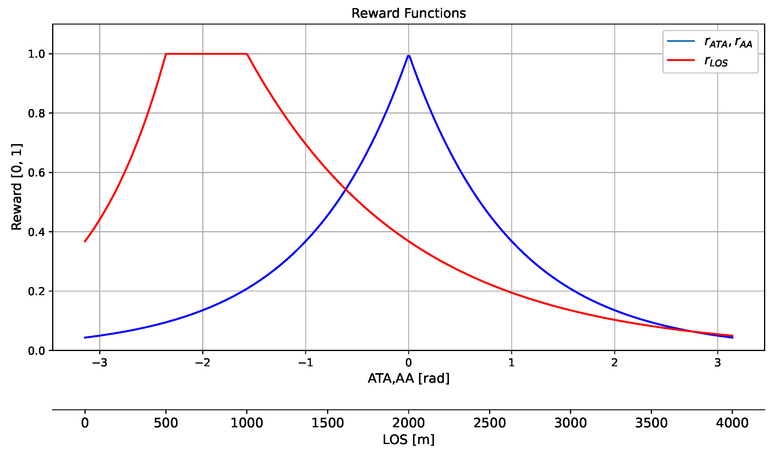
where $w_i$ is the weight of each reward types, and the sum of these weight $\sum w_i$ is equal to 1. An example reward function with weights $w_1=0.4$, $w_2=0.4$, and $w_3=0.2$ is given in Figure 5.

2.3. Deep Q Network

We use the Deep Q Network (DQN) to train our RL agent [43]. The DQN is a reinforcement learning algorithm that combines deep neural networks with Q learning [44], which is a popular method to learn optimal policies in Markov decision processes. The key idea behind the DQN is to use a deep neural network to approximate the Q function, which is computed using the Bellman equation. The Bellman equation expresses the optimal Q value of a state–action pair as the sum of the immediate reward and the discounted Q value of the next state–action pair.

$$Q^{\ast }(s,a)=\mathbb{E}[r+\gamma \underset{a^{\prime }}{max}Q(s^{\prime },a^{\prime })]$$

(19)

where $\mathbb{E}$ is the expected return, s is the current state, a is the chosen action, r is the immediate reward, $\gamma \in [0,1]$ is the discount factor, $s^{\prime }$ is the next state, and $a^{\prime }$ is the action chosen in the next state. The DQN algorithm uses experience replay and a target network to stabilize the learning process and improve the convergence of the Q value function. The Q value function is learned by minimizing the mean square error between the predicted Q value and the target Q value. The loss function for the DQN is defined as

$$L\left(\theta \right)={\mathbb{E}}_{(s,a,r,s^{\prime })\sim \mathcal{D}}\left[{(Q(s,a)-y)}^2\right]$$

(20)

where $y=(r+\gamma {max}_{a^{\prime }}{Q}^{-}(s^{\prime },a^{\prime };{\theta }^{-}))$ is the updated target value, and $\mathcal{D}$ is the replay buffer. $\theta$ and ${\theta }^{-}$ are the neural network parameters of the current Q function and the target $Q^{-}$ function, respectively. The parameters of the neural networks are updated using the stochastic gradient descent ADAM optimizer [45] with the following equation

$$\theta \leftarrow \theta -\alpha {\nabla }_{\theta }L\left(\theta \right)$$

(21)

where $\alpha$ is the learning rate, and ${\nabla }_{\theta }L\left(\theta \right)$ is the gradient of the loss function with respect to $\theta$.

After training is completed, the agent’s policy is constructed such that the action is chosen to maximize the expected return as follows:

$$\pi \left(s\right)=arg\underset{a}{max}Q(s,a)$$

(22)

The full description of the DQN algorithm is given in Algorithm 1. The state space in Equation (13), the action space in Table 1, and the reward function in Equation (18) are used to train the air combat agent with the DQN. The numerical value of reward weights and aircraft model are given in the training details section.

2.4. Reward Decomposition

In conventional reinforcement learning approaches, the reward signal is typically represented as a singular scalar value, as illustrated in Equation (18). This representation inherently lacks the granularity to distinguish between the contribution of different reward types, thereby omitting explicit explainability that could be generated from each reward type. Reward decomposition addresses this limitation by employing a distinct Deep Q Network (DQN) for each reward type. This methodology enables a precise assessment of the contribution of each reward type to the agent’s decision-making process. With reward decomposition, we can show the relative importance of one reward type over another by comparing the Q values of various reward types in each state. The action is selected by first summing the Q values from each DQN associated with different reward types and then selecting the action corresponding to the highest cumulative Q value. This approach effectively prevents the issue of the tragedy of the commons highlighted in [46].

Algorithm 1 Deep Q Network (DQN) Algorithm

1: Initialize replay memory D to capacity N 2: Initialize action–value function Q with random weights $\theta$ 3: Initialize target action–value function $Q^{-}$ with weights ${\theta }^{-}=\theta$ 4: Initialize state $s_0$ randomly 5: for t $=1$, T do 6:     if random(0,1) < $ϵ$ then 7:         $i=1\le i\le n|i\in \mathbb{Z}$ 8:         $a_t=A\left[random\left(i\right)\right]$ 9:     else 10:         $a_t=arg{max}_{a}Q(s_t,a,\theta )$ 11:     end if 12:     Advance environment one step $s_{t+1}$, $r_t$ = $env\left(a_t\right)$ 13:     Store transition $(s_t,a_t,r_t,s_{t+1})$ in D 14:     Sample random minibatch of transitions $(s_j,a_j,r_j,s_{j+1})$ from D 15:     if $s_{j+1}$ is terminal then 16:         Set $y_j=r_j$ 17:     else 18:         Set $y_j=r_j+\gamma {max}_a{Q}^{-}(s_{j+1},a;{\theta }^{-})$ 19:     end if 20:     Perform a gradient descent step on ${(y_j-Q(s_j,a_j;\theta ))}^2$ with respect to $\theta$ 21:     Periodically update weights of target networks: ${\theta }^{-}=\tau \theta +(1-\tau ){\theta }^{-}$ 22: end for

The Bellman equation that describes the optimal decomposed Q value is written as the sum of the immediate reward and the discounted Q value of the next state–action pair.

$$\sum _c{Q}_c^{\ast }(s,a)=\mathbb{E}\left[\sum _c{r}_c+\gamma \underset{a^{\prime }}{max}\sum _c{Q}_c(s^{\prime },a^{\prime })\right]$$

(23)

where symbol $\mathbb{E},s,a,s^{\prime },a^{\prime }$ follows the same notation as in the DQN, c is the reward component index, and $Q_c$ denotes the Q value for component c that only accounts for the reward type $r_c$.

We employed a double DQN training approach to avoid overoptimistic value estimation in the vanilla DQN algorithm [47]. The loss function for the decomposed DQN is defined as

$$L_c\left({\theta }_c\right)={\mathbb{E}}_{(s,a,r,s^{\prime })\sim \mathcal{D}}\left[{(Q_c(s,a)-y_c)}^2\right]$$

(24)

where the updated target value $y_c$ is defined as

$$y_c=\left(r_c+\gamma Q_c^{-}(s^{\prime },a^{\prime };{\theta }_c^{-}\right).$$

(25)

Unlike the vanilla DQN, the next action $a^{\prime }$ in the next state used by the target Q value function is defined as

$$a^{\prime }=arg\underset{a}{max}\sum _c{Q}_c(s^{\prime },a,{\theta }_c).$$

(26)

That is, instead of using the best action from the target Q value function, we use the action chosen by the original Q value function in the next state $s^{\prime }$. The NN weights are updated with the following equation using the ADAM optimizer [45] as

$${\theta }_c\leftarrow {\theta }_c-\alpha {\nabla }_{\theta }{L}_c\left({\theta }_c\right)$$

(27)

After training is completed, the Q value for a given state–action pair is calculated as

$$Q(s,a)=\sum _c{Q}_c(s,a).$$

(28)

For each component-level Q value, the action–value pair is calculated as

$$Q_c\left(s\right)={[Q_c(s,a_1),Q_c(s,a_2),\cdots ,Q_c(s,a_k)]}^T$$

(29)

where k represents the total number of available actions. The policy function used to select an action is defined as

$$\pi \left(s\right)=arg\underset{a}{max}Q(s,a)=arg\underset{a}{max}\sum _c{Q}_c(s,a)$$

(30)

where the total Q value following the policy $\pi \left(s\right)$ is written as

$$Q^{\pi }\left(s\right)=\sum _c{Q}_c(s,\pi \left(s\right))$$

(31)

and finally, the component-level Q value following the policy $\pi \left(s\right)$ is written as

$$Q_c^{\pi }\left(s\right)=Q_c(s,\pi \left(s\right)).$$

(32)

A vector of these component-level Q value functions following the policy $\pi \left(s\right)$ is defined as

$${\mathbf{Q}}^{\pi }\left(s\right)=[Q_1^{\pi }\left(s\right),Q_2^{\pi }\left(s\right),\cdots ,Q_n^{\pi }\left(s\right)]$$

(33)

n denotes the total number of components considered for the decomposition. The vector elements in Equation (33) represent the expected outcomes for each reward type $r_c$ when the agent follows the policy $\pi \left(s\right)$ from state s. By analyzing the Q values associated with their corresponding reward types, we can deduce the agent’s expectations in terms of the semantically meaningful reward types we have defined, thus providing insight into the reasoning behind its decision-making process.

The full description of the double DQN algorithm with reward decomposition is given in Algorithm 2. The double DQN algorithm with reward decomposition was trained using the same state space, action space, and reward functions as those described in the previous section on DQN.

2.5. Training Details

In this section, we provide the actual training details in a comprehensive fashion to help with reproducibility. The fine-tuned hyperparameters and the episode initialization strategy are given in full detail. An agent needs to explore a wide range of situations to increase its competence. We started each episode with a random relative orientation, speed, and distance between two aircraft. This ensured that our agent had explored the entire state space through its training. The aircraft parameters used in our air combat environment are given in Table 2.

Table 2. Aircraft model parameters.

Symbol	Definition	Value	Unit
$K_V$	Velocity gain	2	-
$K_{\chi }$	Heading angle gain	0.6	-
$\mathsf{\Delta }{V}_c$	Commanded delta speed	[−10, 10]	m/s
$\mathsf{\Delta }{\chi }_c$	Commanded delta heading angle	[−20, 20]	degree
V	Velocity state	[100, 250]	m/s
$\chi$	Heading angle state	[−180, 180]	degree

Table 2. Aircraft model parameters.

Symbol	Definition	Value	Unit
$K_V$	Velocity gain	2	-
$K_{\chi }$	Heading angle gain	0.6	-
$\mathsf{\Delta }{V}_c$	Commanded delta speed	[−10, 10]	m/s
$\mathsf{\Delta }{\chi }_c$	Commanded delta heading angle	[−20, 20]	degree
V	Velocity state	[100, 250]	m/s
$\chi$	Heading angle state	[−180, 180]	degree

Algorithm 2 Double Deep Q-Network (DQN) Algorithm with Reward Decomposition

1: Get number of reward component $c\in C$ 2: Initialize replay memory D to capacity N 3: for Each reward component c do 4:     Initialize action–value function $Q_c$ with random weights ${\theta }_c$ 5:     Initialize target action–value function $Q_c^{-}$ with weights ${\theta }_c^{-}={\theta }_c$ 6: end for 7: Initialize state $s_0$ randomly 8: for t $=1$, T do 9:     if random(0,1) < $ϵ$ then 10:         $i=\{1\le i\le n|i\in \mathbb{Z}\}$ 11:         $a_t=A\left[random\left(i\right)\right]$ 12:     else 13:         $a_t=arg{max}_a{\sum }_c{Q}_c(s_t,a,{\theta }_c)$ 14:     end if 15:     Advance environment one step $s_{t+1}$, $r_t$ = $env\left(a_t\right)$ 16:     Store transition $(s_t,a_t,r_c,s_{t+1})$ in D 17:     Sample random minibatch of transitions $(s_j,a_j,r_{c,j},s_{j+1})$ from D 18:     for Each reward component c do 19:         if $s_{j+1}$ is terminal then 20:            Set $y_j=r_{c,j}$ 21:         else 22:            Set $y_j=r_{c,j}+\gamma Q_c^{-}(s_{j+1},arg{max}_a{\sum }_c{Q}_c(s^{\prime },a,{\theta }_c);{\theta }_c^{-})$ 23:         end if 24:         Perform a gradient descent step on ${(y_j-Q_c(s_j,a_j;{\theta }_c))}^2$ with respect to $\theta$ 25:     end for 26:     for Each reward component c do 27:         Periodically update weights of target networks: ${\theta }_c^{-}=\tau {\theta }_c+(1-\tau ){\theta }_c^{-}$ 28:     end for 29: end for

In addition to the constraints specified by the model parameters in Table 2, we also initialized the relative distance randomly within the range of −1000 to 1000 m. The episodic return of the training session and the Q value components are shown in Figure 6. The RL agents were trained using DQN implementation of [48] with the necessary modification for the decomposition of rewards.

The state space vector $\mathbf{s}$ is normalized to a range of $[-1,1]$ with the following vector to maintain stability:

$${\mathbf{s}}_{scal}=\left[4000,4000,4000,\pi ,\pi ,\pi \right].$$

(34)

We performed element wise division with Equation (13) before obtaining the final state space vector used as an input:

$${\mathbf{s}}_{norm}=\mathbf{s}/{\mathbf{s}}_{scal}.$$

(35)

A balanced weight profile was chosen for experiments where the ATA and AA rewards have the same weight and the LOS has a lower weight. The distance values $d_1,d_2$ were taken from the DARPA AlphaDog challenge [1,49]. Individual values of these weights are given in

Table 3. Environment parameters.

Symbol	Value
$w_1$	0.4
$w_2$	$0.4$
$w_3$	0.2
$d_1$	500
$d_2$	1000

and shown in Figure 5. The total reward is calculated by taking the weighted average of the individual rewards as follows:

$$r_{tot}=0.4\ast r_{ATA}+0.4\ast r_{AA}+0.2\ast r_{LOS}$$

(36)

We ran hyperparameter optimization to reduce fluctuation in the episodic return signal and component-level Q value $Q_c^{\pi }$ signal, as shown in Figure 6. The hyperparameters used in this study during training are shared in

Table 4. Hyperparameters for the experiment.

Hyperparameter	Value
Total Timesteps	2,000,000
Learning Rate	$1\times {10}^{-4}$
Buffer Size	1,000,000
Discount Factor ($\gamma$)	0.99
Target Network Update Rate ($\tau$)	1.0
Target Network Update Frequency	10,000
Batch Size	64
Starting Epsilon (${ϵ}_{start}$)	1
Ending Epsilon (${ϵ}_{end}$)	0.05
Exploration Fraction	0.35
Learning Starts	10,000
Training Frequency	8

to help the reader reproduce the results.

In this section, we have covered background information, including details of the air combat environment, agent training with the DQN in this environment, the extension of the DQN approach with reward decomposition, and training details for reproducibility. In the next section, we will use this background information as a foundation for explainability. We will start with local explanation, expand it into global explanation with tactical regions and visualization of global explanation, and then apply these concepts to the air combat environment.

3. Explainability

In the rapidly evolving field of artificial intelligence, the quest for systems that not only perform optimally but are also explainable and transparent has taken center stage. This is particularly true in complex domains, such as air combat, where the decision-making process of AI agents must be both effective and understandable. The concept of explainability in AI seeks to bridge this gap, thus providing insights into the ‘how’ and ‘why’ of an agent’s actions. The explanation can be roughly divided into local and global explanations depending on the scope. Local explanation tries to answer the question of “Why is this action preferable in this state?” Or, it could be in the form of “How much does each reward type contribute to the selected action?” However, a local explanation is harder to follow when looking at dynamic videos [32], which is the essence of air combat, where states change rapidly. In contrast to the local explanation, the global explanation provides insight into the agent’s decision making in a wider range of situations. It tries to present an explanation for the question “Which reward types are dominant in different regions of the state space?” and “What is the relative contribution of each reward type in this region?” In addition to the local and global textual explanation, an explanation can also be provided in visual form, such as through salience maps [10], where the visual explanation shows which pixels are more important for classified objects. Answering these questions or visualizing the agent’s expectation sheds light on its decision-making process. In this section, we frequently use the phrase “reward type” followed by the name of the associated reward name. It is important to note that the explanations provided are derived from the component-level Q values given in Equation (33), which are by design associated with semantically meaningful reward types. This association allows us to directly refer to them as an X reward type in our explanations, as the purpose of reward decomposition is to generate insights using this relationship. For example, when we say that the X reward type is higher, it indicates that the Q value $Q_c$ associated with the reward type X is higher. We consistently apply and repeat this terminology throughout this section to help clarify the explanations.

The objective of providing explanations goes beyond enhancing the comprehensibility of the agent for the user, thereby increasing trust in the agent. It also serves a critical role in identifying potential deficiencies within the agent’s decision-making processes and acts as a cautionary mechanism to notify users whenever the agent’s rationale diverges from user expectations or accepted norms. This contradicts the notion proposed in [50], in which the author argued that value-based explanations are intrinsically problematic. However, offering explanations that facilitate the identification of an agent’s misbehavior remains crucial, thus underscoring that the primary objective of explanations is not just to detail the inner workings of an optimally performing agent. Instead, it serves to enhance understanding and oversight, particularly in instances where the agent’s expectation deviates from expected or desired outcomes.

To increase the user’s trust in the air combat agent, we developed local, global, and visual explanation methods. We provide examples on how to interpret the explanation result, thus showcasing the effectiveness of our approach in understanding the agent’s decision-making process.

First, we introduce local explanations facilitated by reward decomposition, which offer a microscopic view of decision-making processes. The local explanation answers the question “Why is this action preferable in this state?” by showing a contribution of carefully selected semantically meaningful reward types to provide a qualitative explanation. The question of “How much does each reward type contribute to the selected action?” is answered by showing the relative contribution of each reward type to provide a quantitative explanation. This information can be used to understand the agent’s preference or to detect misalignment between the agent and user expectations.

Second, we give the mathematical foundation of our tactical region-based global explanation approach by extending the local explanation with the reward decomposition, thus providing a broader perspective on the dominance of different reward types. Our method seeks to address the pivotal question of “Which reward type is dominant in different regions of the state space?” by identifying the most dominant reward type through an analysis of the average contribution of each reward type within predefined tactical regions. We generate an answer to the question “What is the relative contribution of each reward type in this region?” by comparing the relative contribution of each reward type in each tactical region.

Third, we introduce a global explanation with a tactical region approach to the air combat environment. We described the tactical regions used in air combat to analyze the dominant reward types within each region. Furthermore, we expanded the tactical regions outlined in the air combat literature to encompass all four quadrants, thus demonstrating how explanations can uncover discrepancies in the agent’s expectations across symmetrically identical regions.

Fourth, we introduce a visual explanation approach, in which we employed color coding to represent the ATA–AA–LOS reward types associated with the agent’s expectations, which is represented by $Q_c$, thereby creating color-coded reward type plots. These visuals offer intuitive insight into the global explanation with tactical regions approach. By color coding the agent’s expectations in Equation (33), we developed a global explanation approach that visualizes these expectations, thereby uncovering changes in the agent’s expectation within the varied scenarios of aerial combat.

3.1. Local Explanation

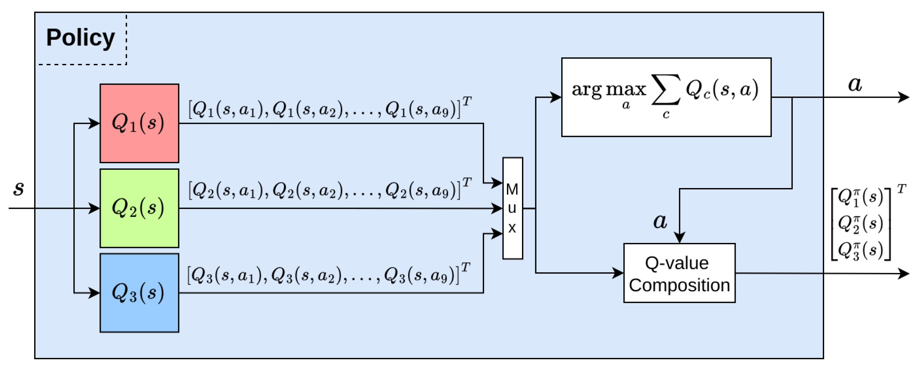
We introduced the explainability to air combat agents using double DQN with reward decomposition in our previous work [42]. Three Q value functions $Q_c$ associated with the ATA, AA, and LOS reward types were obtained after training. These Q value functions are an intrinsic part of the agent’s policy in Equation (30). The block diagram of the agent’s policy is also given in Figure 7.

The explainability was obtained using the Q values given in Equation (33). The Q values associated with the semantically meaningful reward types ATA, AA, and LOS given in Equation (18) provide direct geometrical and tactical relations, thereby making them easy to understand. Recall that the Q value means the return that the agent expects to achieve following its policy. The block diagram of local explainability using decomposed Q values is shown in Figure 8.

We answer the questions of “Why is this action preferable in this state?” by looking at the maximum contribution of the Q value to the selected action using $arg{max}_c{Q}_c^{\pi }$. The answer to “How much doeseach reward type contribute to the selected action?” is obtained directly from the decomposed component-level Q value vector given in Equation (33).

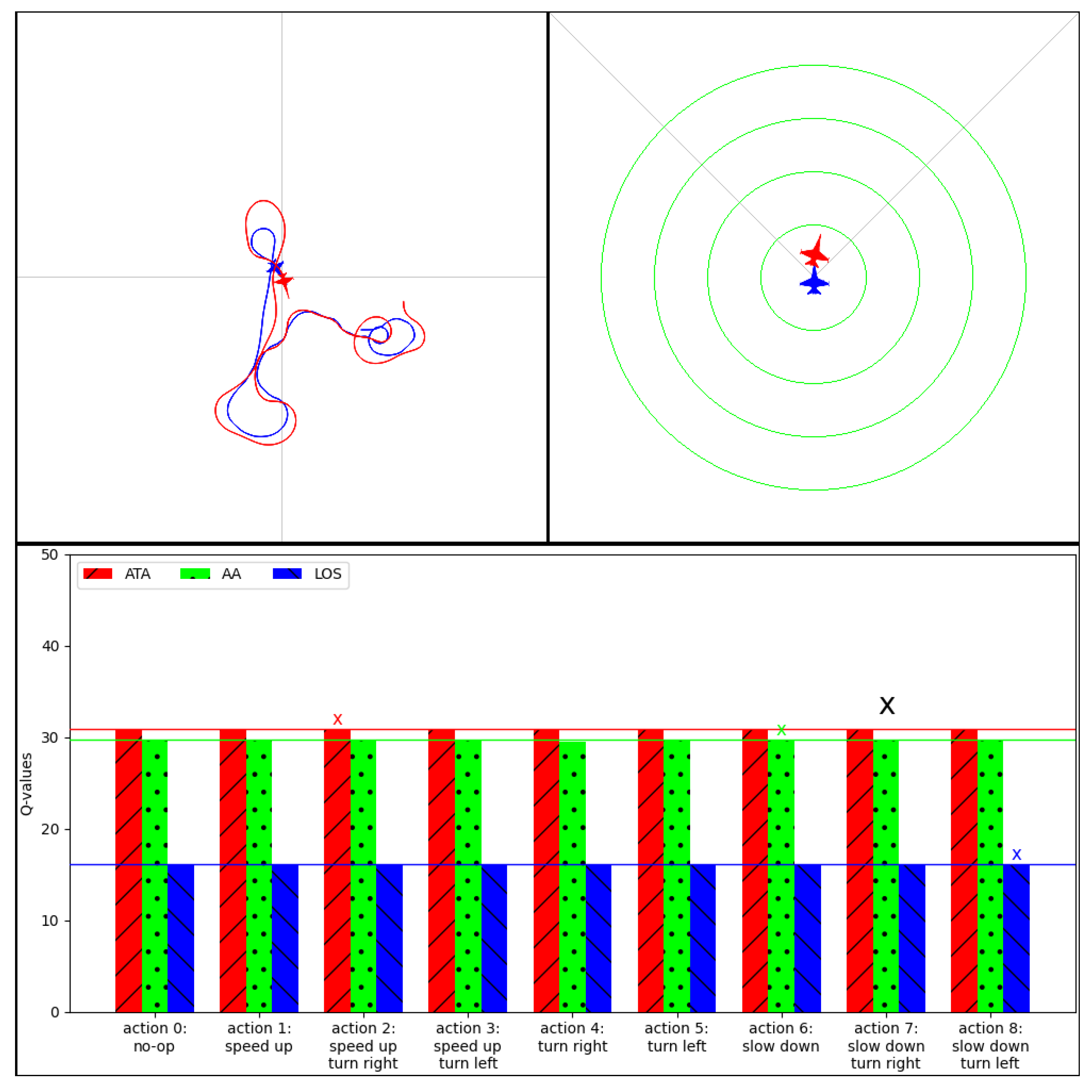
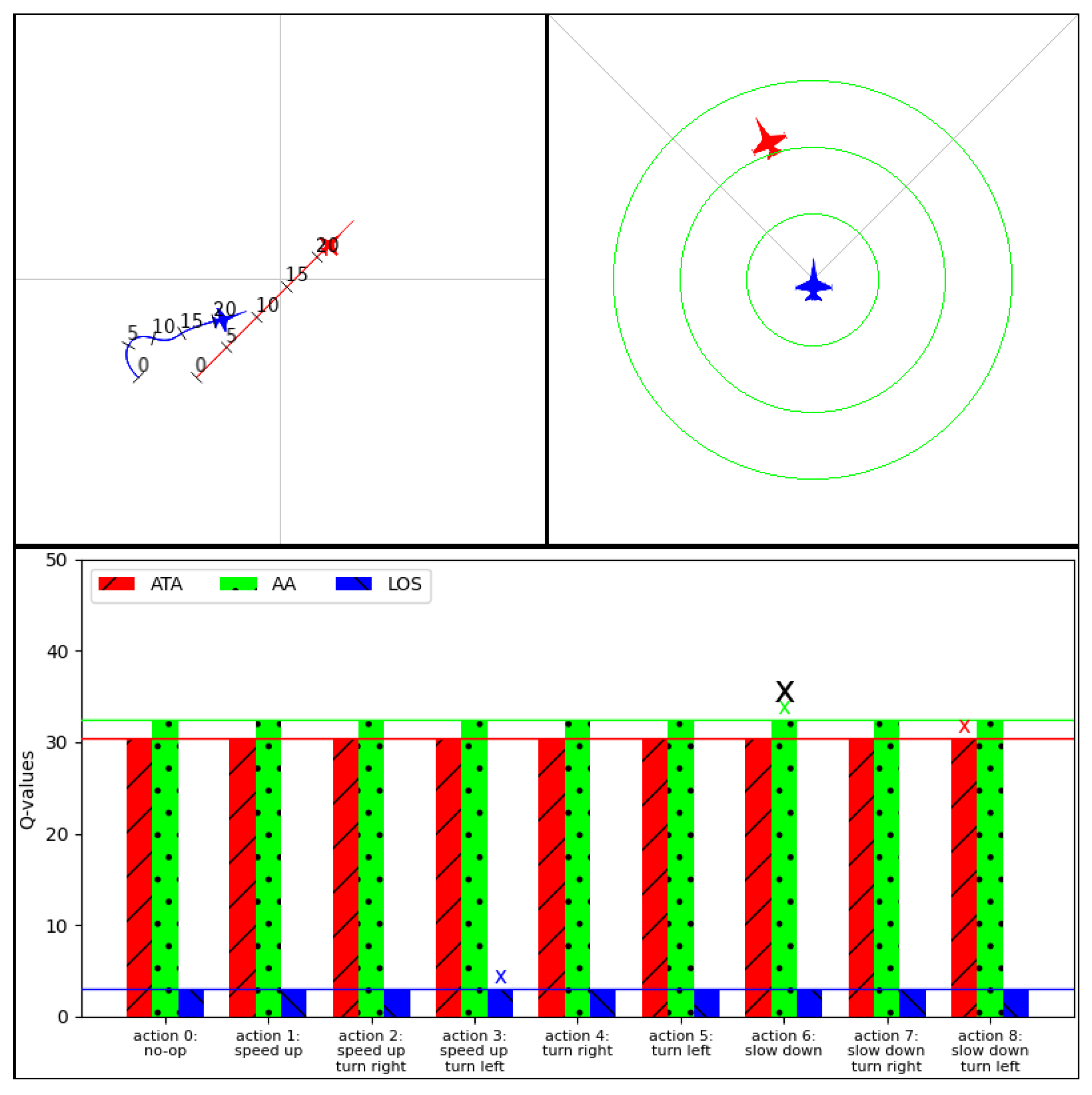
In Figure 9, we show a snapshot of our explainability interface showing the agent’s expectation $Q_c$ for each action and the type of reward $Q_c$ associated with it. Using this information, we can answer the question of why the agent chose to slow down and turn right action while the enemy is within firing range and in front of it. The answer to this question would be that the agent chose this action because it had a higher expectation in the ATA and AA reward types than the LOS reward type, thus meaning that it expected that this action would make it point more towards the target aircraft while also making it stay behind. We could further obtain the contribution of each reward type to the agent’s expectation for the selected action to obtain how much each reward type contributed.

We note that the agent’s expectations for each reward type, even for nonoptimal actions, closely mirrored those of the optimal ones. This suggests that the agent has very similar expectations for all possible actions. We found this outcome to be unexpected, as we anticipated the action to speed up and turn right would have a relatively lower expectation, given that such a maneuver would position the blue aircraft into a more defensive position, thereby effectively placing it in front of the red aircraft.

Even though a local explanation with reward decomposition provides insight into the agent’s decision-making process by showing the agent’s decomposed expectation for each reward type, in a dynamically changing nature of air combat, these values are hard to track and understand. We observed sudden changes in the agent’s expectation in each reward type between temporally close states throughout multiple simulations. To provide a more general overview of the agent’s expectation, we extended the local explanation with reward decomposition to a global explanation with tactical regions.

3.2. Global Explanation with Tactical Regions

The explanation provided by the local reward decomposition does not provide insight into the agent’s preference in neighboring regions. The agent’s expectation for each reward type can change significantly between temporally and spatially similar states. To provide a more general explanation about the agent’s decision-making process, we extended the local explanation with reward decomposition and proposed a global explanation within tactical regions approach. Compared to the question of “Why is this action preferable in this state?” asked in local explanation, we asked “Which reward type is dominant in different regions of the state space?” On a more quantitative basis, instead of the question of “How much does each reward type contribute to the selected action?”, we asked “What is the relative contribution of each reward type in this region?” By identifying the dominant reward type and assessing the relative contributions of each reward type within predefined tactical regions, we highlighted variations in the agent’s expectations and the prevailing rewards influencing its actions. The resultant explanation allows users to better examine the agent’s behavior or provide insight into tactical preference a pilot should have in different tactical regions.

We formalized our explanation approach by first defining tactical regions and the decomposed Q value associated with each reward type:

• Let $\mathcal{T}=\{T_1,T_2,\dots ,T_m\}$ represent the set of tactical regions within the environment, where $j=1,\dots ,m$ indexes each tactical region $T_j$.
• ${\mathbf{Q}}^{\pi }$ in Equation (33) represents the vector of decomposed Q value functions.
• c is the selected reward component.

We first calculate the relative contribution of each $Q_c^{\pi }\left(s\right)$ within a tactical region $T_j$ when the agent follows its policy $\pi \left(s\right)$ as follows:

$$\mathrm{RC}(T_j,{\mathbf{Q}}^{\pi },c)=\frac{{\sum }_{s\in T_j}{Q}_c^{\pi }\left(s\right)}{{\sum }_{s\in T_j}{\mathbf{1}}^T{\mathbf{Q}}^{\pi }\left(s\right)}.$$

(37)

The relative contribution function calculates the proportion of the agent’s expectation for a specific reward type, as shown in Equation (32), in relation to the total expectations for all the reward types given in Equation (31) when following the policy $\pi$. This measure explains the degree to which each reward type influences the selection of the optimal action according to the policy $\pi$, thus revealing the expected return of each reward type within a given tactical region. Dividing the state space into meaningful and manageable tactical regions allows us to understand the agent’s decision-making process in terms of its expectations.

We then define a decision function F that assigns the most dominant reward type to each tactical region, thus identifying the reward type with the highest expectation in each region. Given a vector of decomposed Q value functions following the policy $\pi \left(s\right)$ defined in Equation (33), the decision function F maps each tactical region to the component corresponding to the dominant reward types and is defined as

$$F(T_j,{\mathbf{Q}}^{\pi })=arg\underset{c}{max}\left|\mathrm{RC}(T_j,{\mathbf{Q}}^{\pi },c)\right|.$$

(38)

The decision function aims to elucidate which reward type predominantly influences the actions chosen within a specific tactical region. By considering the absolute value of the relative contribution, our approach accommodates both negative and episodic rewards, thereby broadening its applicability beyond merely continuous-shaped rewards. This adjustment ensures versatility in various reward scenarios, thus enhancing our understanding of action selection across different tactical regions.

This framework quantitatively assesses the influence of different reward types on the agent’s decision-making process within various tactical regions, thereby offering insights into the agent’s expectation. The decision function clarifies “which reward type is dominant in different regions of the state space” by identifying the component c associated with the dominant reward type $r_c$ in the tactical region $T_j$. The decision function reveals that the selection of an action is influenced by the expectation to maximize or minimize $Q_c$ depending on whether the associated reward is positive or negative. This distinction is crucial: a positively defined $Q_c$ suggests that the agent aims for actions that maximize the returns of that reward, while a negatively defined $Q_c$ indicates actions chosen to avoid adverse outcomes. This approach not only answers the question of dominant reward types in various regions but also offers insights into the agent’s expectation associated with each reward type. By linking user-defined semantically meaningful reward types with user-defined tactical regions, we improve the explainability of the agent decision-making process, thus facilitating a deeper understanding of its preference. This approach not only clarifies the underlying rationale of agent behavior but also supports the objectives of explainable artificial intelligence by making complex agent preferences understandable and relatable to users when compared to the detailed but narrower focus of local explanation provided by local reward decomposition. This global perspective enriches our understanding of AI decision-making processes, thereby focusing on context and preference in a way that is immediately accessible to users.

3.3. Global Explanation for Air Combat Tactical Regions

The air combat environment, with its inherent complexity and strategic importance, is well suited for applying the global explanation with the tactical region approach. The distinct tactical regions in air combat allow for a clear analysis of agent behavior through decomposed rewards, thus offering insights into decision making in varied tactical situations.

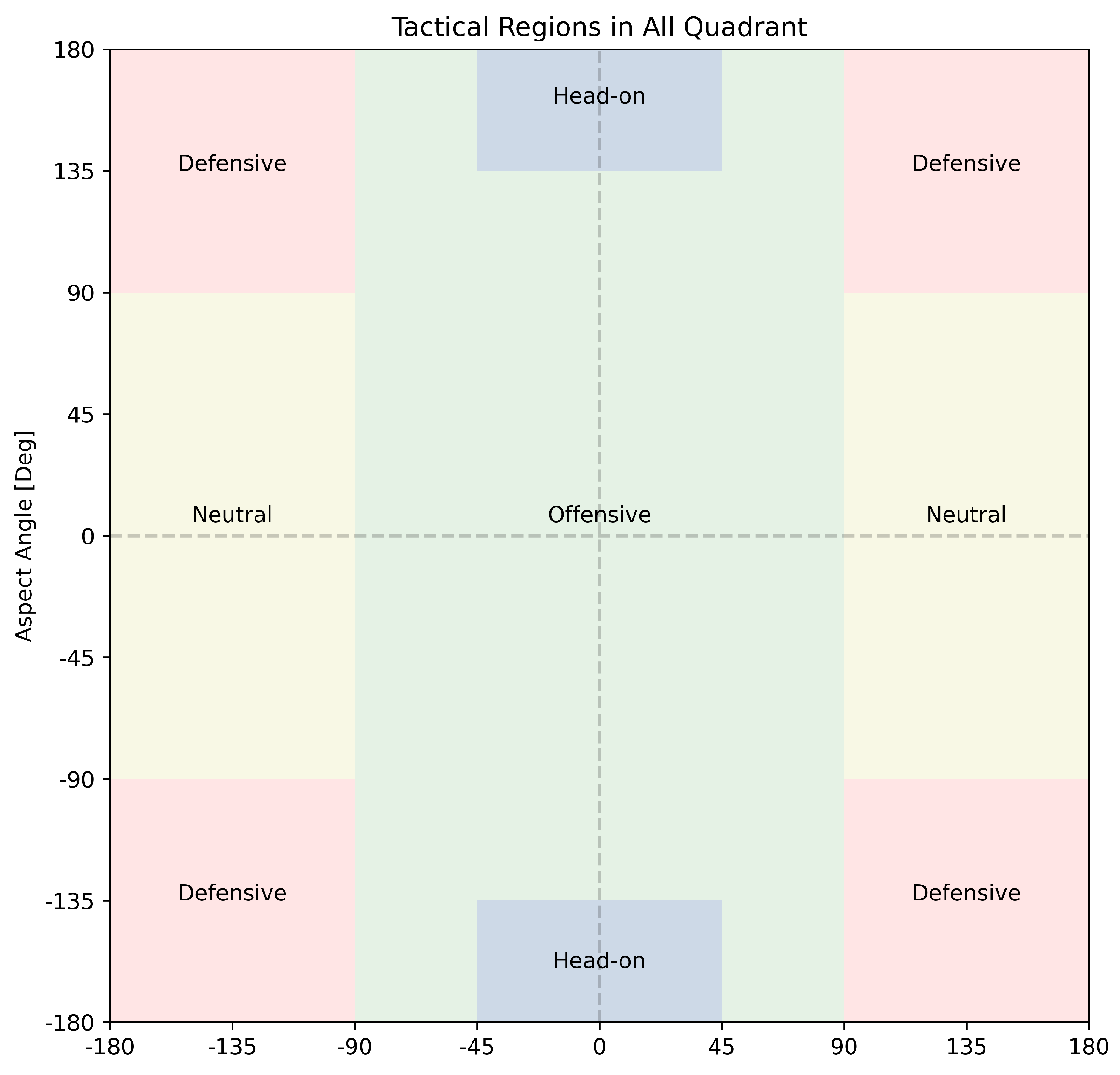
To apply the global explanation with tactical region approach to the air combat environment, we first defined our tactical regions, namely offensive, defensive, neutral, and head-on, as defined within the air combat literature [17,51]. In contrast to the existing literature, we extended the tactical regions to four different quadrants as shown in Figure 10. This extension was introduced to analyze the agent’s expectation in symmetric air combat regions after getting inconsistent results, as shown in Figure 3.

After defining tactical regions, we delineated the boundaries of each tactical region by specifying the criteria that determine the inclusion of states within these designated regions. The offensive region was characterized as where the ATA angle is less than or equal to 90 degrees, thus excluding scenarios that fall within the head-on region criteria. This region signifies the agent’s aggressive positioning, thereby aiming to engage the adversary from advantageous angles. The head-on region was defined by a narrow ATA angle of less than or equal to 45 degrees combined with AA greater than or equal to 135 degrees, thus indicating a direct frontal engagement approach. In contrast, the defensive region was defined as when both ATA and AA angles are greater than 90 degrees, thus suggesting the agent is in a position more susceptible to adversary actions and potentially focusing on evasive maneuvers. Lastly, the neutral region was defined as ATA angles greater than 90 degrees and AA angles less than 90 degrees, thereby representing scenarios where neither party has a distinct offensive advantage. The graph of the regions is shown in Figure 10.

Using these classifications, we defined the set of tactical regions and the set of decomposed Q values associated with specific reward types for air combat, as outlined in Equation (18): $Q_1\sim r_{ATA}$, $Q_2\sim r_{AA}$, and $Q_3\sim r_{LOS}$. Let $\mathcal{T}=\{T_{offensive},T_{defensive},T_{neutral},T_{head-on}\}$ be the set of tactical regions, and let ${\mathbf{Q}}^{\pi }=\{Q_1^{\pi },Q_2^{\pi },Q_3^{\pi }\}$ be a vector of component-level Q value functions in the air combat environment. Based on the tactical region definition given above and the state vector in Equation (13), we further defined the set of states corresponding to each tactical region as follows:

$$\begin{array}{cc}\hfill T_{\text{head-on}}& =\left\{s\in \mathcal{S}\mid \mathrm{ATA}\left(s\right)\le {45}^{\circ }\wedge \mathrm{AA}\left(s\right)\ge {135}^{\circ }\right\}\hfill \end{array}$$

(39)

$$\begin{array}{cc}\hfill T_{\mathrm{offensive}}& =\left\{s\in \mathcal{S}\mid \mathrm{ATA}\left(s\right)\le {90}^{\circ }\wedge s\notin T_{\text{head-on}}\right\}\hfill \end{array}$$

(40)

$$\begin{array}{cc}\hfill T_{\mathrm{defensive}}& =\left\{s\in \mathcal{S}\mid \mathrm{ATA}\left(s\right)>{90}^{\circ }\wedge \mathrm{AA}\left(s\right)>{90}^{\circ }\right\}\hfill \end{array}$$

(41)

$$\begin{array}{cc}\hfill T_{\mathrm{neutral}}& =\left\{s\in \mathcal{S}\mid \mathrm{ATA}\left(s\right)>{90}^{\circ }\wedge \mathrm{AA}\left(s\right)\le {90}^{\circ }\right\}\hfill \end{array}$$

(42)

where $T_{\text{head-on}},T_{\mathrm{offensive}},T_{\mathrm{defensive}},$ and $T_{\mathrm{neutral}}$ directly represent the sets of states corresponding to each tactical region. Functions $\mathrm{ATA}\left(s\right),\mathrm{AA}\left(s\right),$ and $\mathrm{LOS}\left(s\right)$ are selector functions that return the respective values for a given state s, as defined in Equation (13).

Following Equations (37) and (38), we calculated the dominant reward types and their relative contribution for all the tactical regions and quadrants shown in Figure 10. The resulting explanation in terms of the dominant reward type and relative contribution of each reward type when the LOS was at 2000 m is given in

Table 5. Tactical regions reward dominance at LOS 2000 m.

Tactical Region	Dominant Reward Type	Relative Contribution
1st Quadrant
Head-on	ATA	[0.388, 0.315, 0.298]
Offensive	ATA	[0.476, 0.330, 0.195]
Defensive	ATA	[0.414, 0.288, 0.298]
Neutral	AA	[0.386, 0.511, 0.103]
2nd Quadrant
Head-on	ATA	[0.384, 0.341, 0.276]
Offensive	ATA	[0.486, 0.315, 0.199]
Defensive	ATA	[0.434, 0.195, 0.370]
Neutral	ATA	[0.461, 0.380, 0.159]
3rd Quadrant
Head-on	ATA	[0.398, 0.310, 0.292]
Offensive	ATA	[0.458, 0.355, 0.188]
Defensive	ATA	[0.400, 0.298, 0.302]
Neutral	AA	[0.366, 0.539, 0.095]
4th Quadrant
Head-on	ATA	[0.423, 0.285, 0.292]
Offensive	ATA	[0.508, 0.271, 0.220]
Defensive	ATA	[0.387, 0.241, 0.371]
Neutral	ATA	[0.462, 0.395, 0.143]

. To reiterate, this agent was trained using the weight of 0.4 for the ATA and AA the reward and weight of 0.2 for the LOS reward.

In applying the global explanation with the tactical region approach to the air combat environment, we uncovered nuanced insights into the agent’s decision-making processes. The following examples illustrate the practical implications of this analysis, from identifying the dominant reward types within specific regions to exploring variations in agent expectations across symmetrical tactical regions and leveraging this knowledge to debug and realign the agent’s strategies. Each example serves to demonstrate the depth of understanding we can achieve regarding the agent’s decision-making process.

The 1st quadrant results are analyzed for this example explanation. In the head-on, offensive, and defensive regions, the ATA was identified as the dominant reward type. Since the ATA measures how directly our aircraft faces the target, the result suggests that in these tactical areas, the agent’s selected actions are based on the expectation of maximizing the ATA reward. This interpretation implies that the agent expects that its actions will result in better alignment with the target aircraft. Furthermore, in the neutral region, the dominant reward type changed to the AA, thus indicating that the agent expects the selected actions to position it more advantageously behind the target aircraft. Delving deeper into the analysis to examine the relative contribution of each reward within specific tactical regions reveals nuanced reasoning. In the head-on and defensive regions, the AA and LOS rewards contributed approximately $30\%$ each. However, when transitioning from the head-on region to the defensive region, the contribution from the ATA reward increased by an additional $7\%$. This change suggests that, while the agent has similar expectations for all reward types in the head-on region, thus recognizing the tactical disadvantage of its positioning, it considers actions that enhance the ATA reward to be more critical in the defensive region to improve its offensive stance and potential to land hits. This insight into the dominant reward type and the relative contribution of each reward type underscore how the agent’s expectation can be used to explain its decision-making process with this framework, and the reward weight used during training did not translate fully to the trained agent.

The 1st and 3rd quadrants represent symmetric geometries in air combat scenarios, with the agent’s aircraft oriented left and right of the line of sight in the 1st and 3rd quadrants, respectively, with the target aircraft oriented oppositely. Analyzing the tactical regions within these quadrants uncovers distinct variations in agent expectations. Specifically, in the neutral region of both the 1st and 3rd quadrants, the AA reward was predominant; however, the relative contribution between these regions was different for each reward type. This change in relative contribution between symmetrical regions indicates that the agent’s expectations can differ even in geometrically identical scenarios. Such discrepancies point to potential inconsistencies in the agent’s policy and an imbalance in training, thereby possibly stemming from the random initialization process. The use of dominant rewards and their relative contributions as an explanatory tool enables the identification of these inconsistencies through direct analysis of the agent’s policy, thus bypassing the need for extensive simulation. This method provides a clear window into the agent’s decision-making process, thereby highlighting areas for potential improvement or adjustment.

The evaluation of dominant rewards across tactical regions provides a vital mechanism for debugging the agent and identifying any discrepancies between the agent’s expectation and the expectations of a human operator. Consider the defensive region within the 1st quadrant, where the ATA reward dominated; in contrast to this, a human operator might anticipate a higher preference for the AA reward, thereby suggesting a cautious strategy aimed at positioning behind the target rather than directly engaging it. Similarly, the prevalence of the AA reward in the neutral region of the 1st quadrant stands out. In such a scenario, where neither party holds a clear positional advantage, a dominant expectation towards the AA reward might indicate a more defensive posture, thus hinting that the agent is adopting a less aggressive approach in this tactically ambiguous region. These examples highlight how an analysis focused on dominant rewards can pinpoint areas where the agent’s expectation deviates from user expectation, thereby offering clues for further investigation and refinement. This approach of examining reward dominance and distribution across tactical regions, coupled with comparisons with human pilot expectations, establishes a robust framework for debugging and ensuring alignment. By highlighting areas where the agent’s expectation diverges from the one expected by the human operator, it allows for the critical assessment and adjustment of the agent’s tactic, thus ensuring that its actions are in concordance with established tactical principles and human expertise.

3.4. Global Visual Explanation

The visual explanation approach provides a more granular and qualitative perspective on the agent’s decision-making process, thus offering insights that extend beyond the averaged reward dominance per area, as shown in the global explanation with tactical region approach. This method uncovers subtle variations and patterns in the agent’s expectations that may not be immediately evident from the aggregated data by visually representing the color-coded agent’s expectation value across the state space. This approach uses color-coded heat maps based on normalized Q values. By mapping the relative importance of different Q value components to a spectrum of colors, this method provides immediate visual insight into the agent’s decision-making process across various tactical regions. Such a visual representation not only enhances our understanding of the agent’s decision-making process but also facilitates the identification of areas for improvement, thereby enabling a more informed and targeted approach to refining agent performance and alignment with desired outcomes. Due to the inherent limitations of color coding, this approach is currently restricted to visualizing a maximum of three reward types.

The equation provided outlines the process to generate color-coded visual explanations that reflect the agent’s expectations based on its policy $\pi \left(s\right)$ across different states s. Specifically, the magnitude of component-level Q values $(Q_1^{\pi }\left(s\right),Q_2^{\pi }\left(s\right),$ and $Q_3^{\pi }\left(s\right))$ for a given state is normalized against the maximum absolute value between these components. This normalization process ensures that each contribution of the Q value component is proportionally represented, with the maximum contributing component scaled to unity. The resulting normalized values are then mapped onto the RGB color space, where each component corresponds to one of the primary colors (red, green, or blue).

$$\mathrm{Color}(s,{\mathbf{Q}}^{\pi })=\frac{\left[|Q_1^{\pi }\left(s\right)|,|Q_2^{\pi }\left(s\right)|,|Q_3^{\pi }\left(s\right)|\right]}{{max}_c\left|Q_c^{\pi }\left(s\right)\right|}·\left[\begin{array}{ccc}1& 0& 0\\ 0& 1& 0\\ 0& 0& 1\end{array}\right],c\in \{1,2,3\}$$

(43)

This mapping transforms numerical data into a visual format, thus allowing us to intuitively understand the relative influence of each Q value component on the agent’s decision-making process at any given state. Through this approach, the visualization directly communicates the agent’s prioritized expectation, thereby offering insights into its decision-making process and highlighting areas of potential refinement. Taking the absolute value of both the numerator and the denominator makes this visualization technique immune to the sign of the reward, thus making it equally applicable and informative for both positive and negative reward scenarios. This ensures that the method provides valuable information regardless of the reward structure used for training. Similar to the application of global explanation with tactical region approach to air combat, the relation between Q values, reward types, and color coding is as follows:

$$\begin{array}{c}\hfill \begin{array}{cc}\hfill Q_1\sim & r_{ATA}\sim \mathrm{RED}\hfill \\ \hfill Q_2\sim & r_{AA}\sim \mathrm{GREEN}\hfill \\ \hfill Q_3\sim & r_{LOS}\sim \mathrm{BLUE}.\hfill \end{array}\end{array}$$

(44)

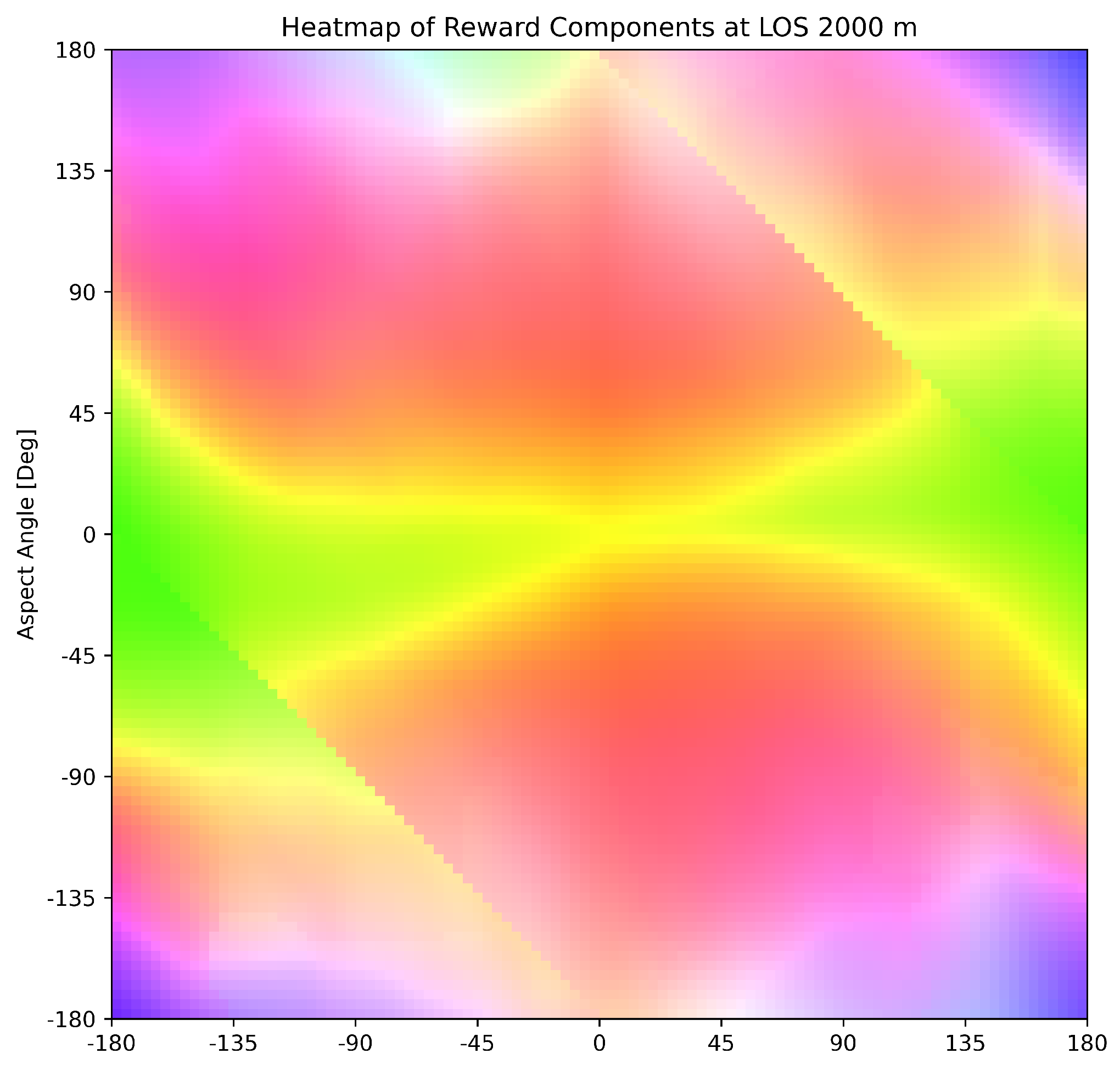
The comparison between the visual explanations shown in Figure 11 and the quantitative data presented in Table 5 demonstrates a clear correlation. For example, in the upper right 1st quadrant, the ATA (represented in red) emerged as the predominant reward type in both the offensive and the head-on regions, thereby aligning with the findings in Table 5. In the defensive region, we can observe a balanced contribution across all reward types, with a preference towards the ATA (red). Conversely, the AA reward type (depicted in green) was more pronounced in the neutral region, thus underscoring its dominance as identified in the table. While this analysis specifically focuses on the first quadrant, a similar consistency in reward type dominance and distribution was evident across the entire color map, thereby reinforcing the alignment between the visual and tabulated explanations of the agent’s decision-making process.

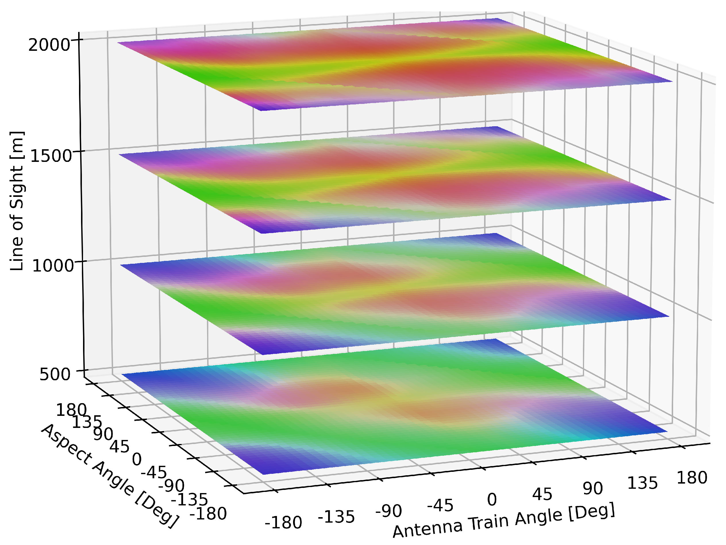
The utility of this visual explanation becomes particularly apparent when identifying areas within the state space where the agent’s expectations deviate from anticipated symmetrical outcomes. For illustrative purposes, the state space was sampled at fixed Line of Sight (LOS) distances of 500, 1000, 1500, and 2000 m with variations in the ATA and AA values, as demonstrated in Figure 12. The figure reveals that as the distance between the aircraft decreased, the discrepancies in agent expectations across symmetric quadrants began to diminish. This observation suggests a convergence in the agent’s expectation as combat scenarios become more proximate, thus highlighting the impact of spatial dynamics on the agent’s decision-making process.

We used the color coding from Equation (43) to present the change in agent expectation along the trajectory defined by the ATA, AA, and LOS states. It is important to note that the ATA, AA, and LOS states, as defined in Equations (9)–(11), differed from the ATA, AA, and LOS reward types specified in Equation (18). Although the reward functions were derived from these states, the states themselves represent the spatial domain the agent navigates, and the reward types are the signals used by the agent to train its policy. We compared the simulation results of the symmetric initial states, both of which resided in the neutral region. In the first simulation, the headings of both aircraft were oriented so that the initial ATA state was −135 degrees and the AA state was 45 degrees, which corresponds to the neutral region in the 2nd quadrant. The second simulation started with an ATA state of 135 degrees and an AA state of −45 degrees, which corresponds to the neutral region in the 4th quadrant. In both simulations, the aircraft were positioned 1000 m away from each other, and the initial velocity was set to 150 m/s. The red target aircraft was set to move along a straight line for demonstration purposes.

In the initial simulation shown in Figure 13, the trajectory analysis from a bird’s-eye view highlights the agent’s maneuvers towards the target aircraft. Between 0 and 10 s, the agent executed a sharp left turn and then accelerated to close the distance for engagement while slowly adjusting its heading. The change in the contribution of each Q value to the selected actions over this period began with similar relative contributions from all Q values, as shown in the bottom plot. The ATA reward type became dominant during the sharp turn and settled after 8 s once the agent completed its maneuver and aligned with the target aircraft. This indicates that alignment with the target aircraft was the main contributor to the selected actions. The upper right plot reveals that the agent increased its speed and approach towards the target aircraft, as evidenced by the decreasing LOS state values from 2000 m to 1000 m in the upper right plot. The LOS reward type contribution gradually increased during this time, thus indicating a correct change in the agent’s expectation as it narrowed the distance with the target.This observation shows the tactic adopted by the agent, which balanced between alignment (ATA) for offensive positioning and distance closure (LOS) to maintain or enter the engagement range.

However, in the second simulation, despite starting from geometrically symmetrical states, the agent did not get close to the target aircraft after a sharp right turn, as shown in Figure 14. The lower plot shows that the agent had expectations similar to the first simulation in the first 10 s. After 10 s, the expectation of the LOS reward decreased. Although the agent had a correct expectation aligning with the change in LOS state, it did not choose the speed-up action.

The snapshot of the local reward decomposition taken after 20 s shown in Figure 15 reveals that the aggregated expectation had the highest value in the slowdown action, which was dominated mainly by the AA reward, similar to the lower plot in Figure 14. However, the Q value associated with the LOS reward type had the highest value for the speed-up turn left action. The two contradictory slow-down and speed-up actions when the two aircraft were far away indicate a problem with the agent policy. Investigating agent’s decision making and obtaining this kind of explanation would not be possible without the reward decomposition method.

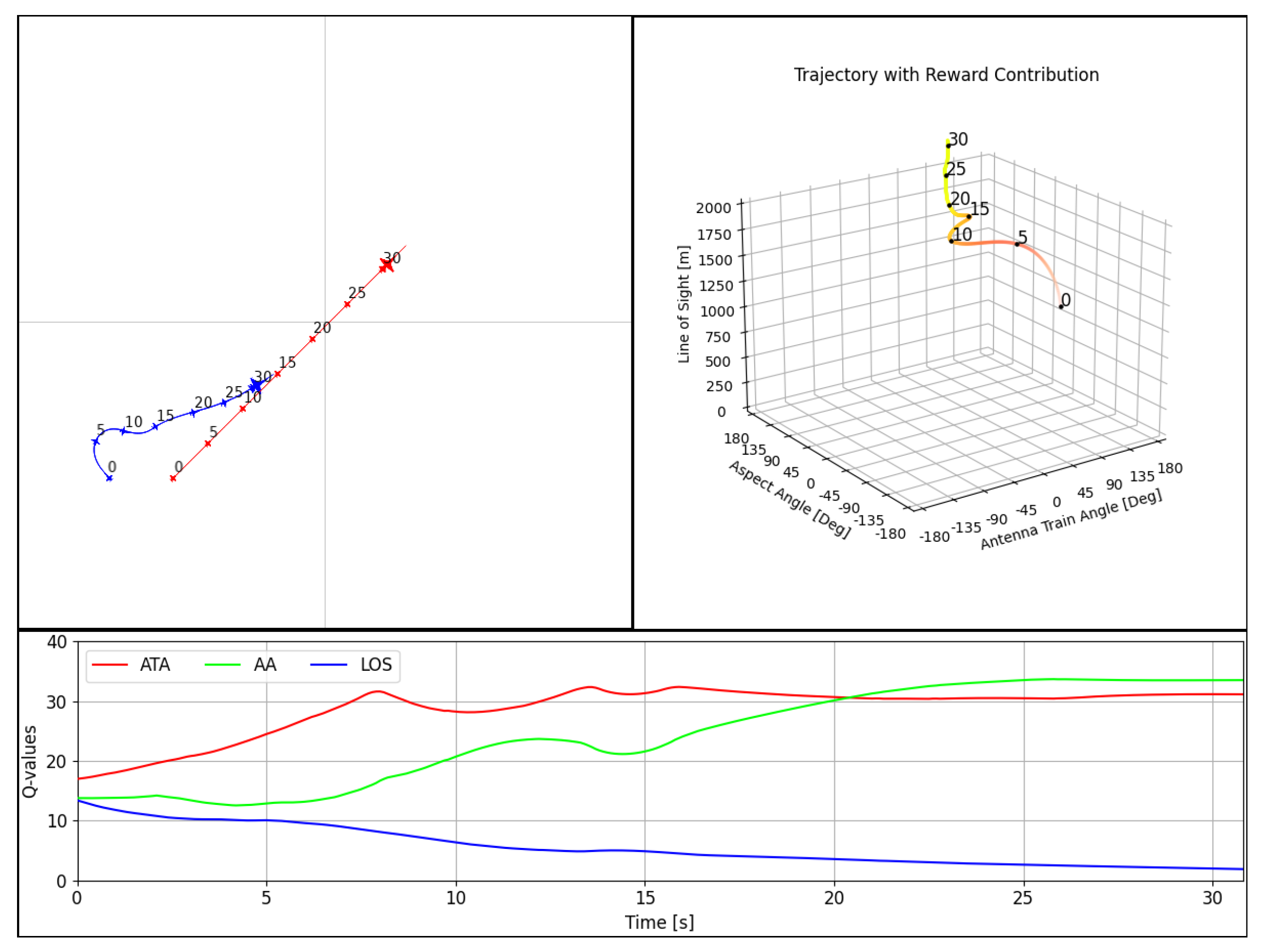
Similarly to the previous example, a trajectory-based explanation is provided to show the agent’s decision-making process over time during an air combat engagement where the same agent is pitted against itself. In this simulation run, the blue aircraft was positioned at $(-500,500)$, and the red aircraft was positioned $(500,500)$ with the heading of $-90$ degrees. The initial velocity was set to 150 m/s. To reiterate, the agent was trained against a randomly moving aircraft, with each episode starting from randomly selected initial states, and the Q value of each reward type represents the agent’s expected return starting from given state while following its policy. The result of this simulation is given in Figure 16.

We can observe in the bird’s-eye view (upper left plot) that the agent kept its course constant in the first 5 s and executed a sharp left turn towards the target between 5 and 10 s. The AA reward type increased during the constant course phase followed by the increase in the ATA (red line) reward type, as shown in the lower plot. This suggests that the agent expected such a maneuver to first place it behind the target aircraft and then align itself towards it. A similar observation can also be made with the upper right plot, which shows the color-coded Q value contribution in 3D whose axes are the ATA–AA–LOS state. The color-coded trajectory was initially white, thus indicating that the agent had a similar expectation for all reward types. This was followed by the green color at around 5 s, thus indicating a high expectation for the AA reward type, and the orange color around the 10 s mark, thus indicating a similar expectation for the ATA and AA reward types.

The blue aircraft closed its distance with the target between 10 and 20 s while keeping its heading fixed to the target, thus performing a pure pursuit maneuver. The target aircraft made a right turn between 20 and 30 s, thus making the blue aircraft overshoot in its course, and the fight went into to lag pursuit, which resulted in a lower expectation for the ATA Q value. The blue aircraft made a sharp right turn to align its heading with the red aircraft and speed up while continuing its pure pursuit maneuver. The red aircraft also maximized its speed to escape pure pursuit. Since the two aircraft had identical dynamics, neither could gain an advantage after this point. The simulation was finished at the 55 s mark, because the two aircraft entered a rate fight. It should be noted that, even though the simulation started from an equally offensive position for both aircraft and they were driven by the same agent, the blue aircraft maintained its offensive stance better than the red one. Similarly to the previous example, this shows the importance of testing for symmetrical air combat geometries.

In this section, we presented various explanation approaches, including local explanation, global explanation with tactical regions, visualization of the global explanation, and its application to the air combat environment. In the next sections, we provide a discussion and conclude the paper by summarizing our findings and suggesting future research directions.

4. Discussion

Most studies in the air combat literature focus on developing optimal agents using policy-based reinforcement learning approaches, which typically do not provide mechanisms to generate global intrinsic explanations. This is a significant limitation in operational settings, where understanding the rationale behind AI decisions is crucial to trust and engage in effective human–AI collaboration. In contrast, our work introduces a novel explanation approach that extends intrinsic local explanations to global explanations with tactical regions using the reward decomposition of a value-based Deep Q Network. Our study not only demonstrates the successful application of agents in various air combat scenarios but also allows for the generation of comprehensive and meaningful explanations that can be easily interpreted by users.

The novel approach to explainability developed in this work addresses a critical gap in Explainable Reinforcement Learning (XRL) by providing mechanisms for generating global intrinsic explanations that are suitable for dynamic and continuously changing environments where local explanation methods fall short. By segmenting the state space into semantically meaningful tactical regions, our method improves the relevance and comprehensibility of the explanations that enable a broader evaluation of agent decision-making processes. This segmentation can significantly improve user understanding without the need for exhaustive simulations.

Furthermore, our approach offers substantial practical implications in domains where quick and reliable decision making is paramount. Our method improves operational readiness by providing clarity on AI-driven decisions, thereby improving coordination and strategic planning. Additionally, the principles established here could be adapted to other complex, dynamic environments such as autonomous driving and robotic navigation, where understanding AI behavior in diverse scenarios is critical.

In broader terms, this work significantly advances the field of XRL. Not only does it provide approaches for the deeper integration of AI systems in high-stakes environments, but it also sets a foundation for future research into the development of explainable AI across various domains. The explanation methods developed here could lead to more robust, transparent, and trustworthy AI systems, thus paving the way for their adoption in more critical and public-facing applications.

5. Conclusions

This work contributes to the field of explainable reinforcement learning (XRL) by extending local explanation methods to a global context through the innovative use of tactical regions and by introducing a visual explanation approach for decomposed rewards. We demonstrated the effectiveness of our approaches in providing nuanced insights into the agent’s decision-making processes by applying them to a complex and dynamic air combat environment. Our findings reveal that by analyzing dominant reward types and their distributions across different tactical regions, we can gain a deeper understanding of an agent’s decision-making process and identify areas for potential improvement. The visual explanation technique, with its color-coded representation of reward types, further enhances our ability to intuitively grasp the agent’s expectations, even in scenarios where traditional explanations might fall short. These contributions not only advance the state of XRL research but also have practical implications for the design and evaluation of AI systems in high-stakes domains, thus emphasizing the importance of explainability for trust, transparency, and alignment with human strategic objectives.

Future work includes expanding the global explanation with tactical regions approach to other reinforcement learning architectures. Another research direction would be to conduct extensive empirical user studies to validate the proposed approach. These future works will further the utility of XRL in complex dynamic environments, thereby contributing to the development of highly performing, transparent, and trustworthy autonomous systems.