Stealth Aircraft Penetration Trajectory Planning in 3D Complex Dynamic Based on Radar Valley Radius and Turning Maneuver

Abstract

Based on the quasi-six-degree-of-freedom flight dynamic equations, considering the changes in the elevation angle caused by an increase in the rolling angle during maneuvering turns, which leads to a rise in the radar cross-section. A computational model for the radar detection probability of aircraft in complex environments was constructed. By comprehensively considering flight parameters such as turning angle, rolling angle, Mach number, and radar power factor, this study quantitatively analyzed the influence of these factors on the radar detection probability. It revealed the variation patterns of radar detection probability under different flight conditions. The results provide theoretical support for the Radar Valley Radius and Turning Maneuver Method (RVR-TM) based on decision trees, and lay the foundation for the development of subsequent intelligent decision-making models. To further optimize the trajectory selection of aircraft in complex environments, this study combines theoretical analysis with reinforcement learning algorithms to establish an intelligent decision-making model. This model is trained using the Proximal Policy Optimization (PPO) algorithm, and through precisely defining the state space and reward functions, it accomplishes intelligent trajectory planning for stealth aircraft under radar threat scenarios.

1. Introduction

With the continuous advancement of radar detection technology, the stealth performance of aircraft has become a key factor in their survivability. Traditional stealth designs have primarily focused on the aircraft’s geometric shape and stealth materials to reduce its Radar Cross Section (RCS). However, as counter-stealth technologies have upgraded, relying solely on RCS as a static indicator to evaluate the stealth performance of aircraft is no longer sufficient to meet the complexity and dynamism of modern battlefield environments. Therefore, analyzing the stealth performance of aircraft from a dynamic perspective, considering the influence of their attitude, speed, and trajectory variations during actual flight on RCS, has become a new direction in stealth technology research.

Many scholars have delved into the development of trajectory planning methods of stealthy penetration. Moore FW [1] devised a strategy to minimize peak and cumulative RCS for autonomous precision-guided munitions. Similarly, Liu et al. [2] presented an integrated approach combining multi-phase optimal control theory with the adaptive pseudo-spectral method to engineer stealthy trajectories. Hao et al. [3] proposed a 3D trajectory planning technique employing the A* algorithm, specifically designed for low-altitude penetration in the context of dual-radar threats. The paper utilizes a cost function for the A* algorithm that correlates with the average radar intensity, which offers a simplified representation of the threat landscape with certain limitations in precision. Zhang et al. [4] introduced a dynamic RCS model-based algorithm for real-time trajectory planning of stealthy UAVs tailored for an ellipsoidal shape. Mi et al. [5] developed a stealth trajectory planning framework leveraging the sparse A* algorithm, considering the constraints of the threat environment. Further, Guan et al. [6] expanded upon the A* algorithm by incorporating the log-normal RCS model proposed by Lu et al. [7], leading to the introduction of the 3D Sparse A* Log-normal radar model (3D-SASLRM), which is grounded in the log-normal radar model.

Search-based trajectory planning methods often require substantial computational resources for trajectory searching and constructing trajectories that meet penetration requirements. In such searches, many computational resources are used to attempt ineffective trajectories. Therefore, employing a priori knowledge and the most effective methods for trajectory planning can significantly reduce search time and improve planning efficiency. Utilizing the concept of the radar valley radius proposed by Guan et al. [6] and the turning maneuver penetration method proposed by Lu et al. [7] enables rapid trajectory planning.

In addition to search-based trajectory planning methods and rapid trajectory planning based on a priori knowledge, an increasing number of researchers are utilizing reinforcement learning, a method that closely resembles human experiential learning, to accomplish the trajectory planning for various intelligent agents such as aircraft, robots, and underwater vehicles [8,9,10,11,12,13,14,15,16,17,18,19]. Currently, a small number of researchers have begun to apply reinforcement learning to stealth penetration decision making. The most fundamental application is in countering radar tracking, where numerous input stimuli exist, and the rewards are relatively dense. Alpdemir [20] proposed a deep reinforcement learning solution for the trajectory planning problem of tactical unmanned aerial vehicles under the threat of radar tracking, integrating a Markov Decision Process with a variant of Deep Q-Networks and prioritized experience replay, along with Learning from Demonstrations (LfD). Wang Z [21] and colleagues introduced a Concealment–Distance Dynamic Weight Deep Q-Network algorithm for the three-dimensional trajectory planning of unmanned helicopters, which considers radar and infrared detection threats and optimizes trajectory planning outcomes through a dynamic weighting reward function. Through comparative analysis, Hameed et al. [22] studied the application of deep reinforcement learning algorithms in aircraft avoidance or the minimization of radar detection and tracking, finding that the Proximal Policy Optimization (PPO) algorithm generally performs better. In scenarios where only radar detection is considered, and the reward is the sparsest, Ma Zijie et al. [23] proposed an improved deep reinforcement learning algorithm to enhance cruise missiles’ penetration trajectory planning capability when facing dynamic early warning radar threats. Wang Y et al. [24] combined Task Completion Division (TCD) with the Soft Actor-Critic (SAC) algorithm to form the TCD-SAC algorithm, proposing a reinforcement learning method based on an improved sampling mechanism to enhance the penetration capability of unmanned aerial vehicles in air defense systems, with the improved sampling mechanism effectively mitigating the training difficulties caused by sparse rewards.

In this paper, using the aerodynamics, engine, and RCS data of a flying wing aircraft, and referring to prior knowledge from the analysis of the turning maneuver in the 3D scene, we propose a Radar Valley Radius and Turning Maneuver Method (RVR-TM method) for aircraft penetration trajectory planning in dynamic complex environments. This method first outlines a pre-planned trajectory based on the radar valley radius, then calculates the aircraft’s relative angle to the radar and employs a maneuver-turning method to adjust the trajectory at points where the aircraft is most exposed to the radar, thereby reducing the radar detection probability across the entire trajectory. The results are then compared with the trajectory planning outcomes of the A* algorithm. Building upon the research on stealth aircraft penetration, we proposed an intelligent decision-making model based on the reinforcement learning PPO algorithm. Trajectory planning simulations were conducted in a single-radar scenario to study the influence of incorporating distance and action penalties in the planned trajectories.

2. Models

Before guiding the penetration of stealth aircraft, it is necessary to specify the RCS, aerodynamic calculation, and engine models used in the computation process. This study employs a typical flying wing aircraft configuration, with the specific details provided below.

2.1. Three-Dimensional RCS Model

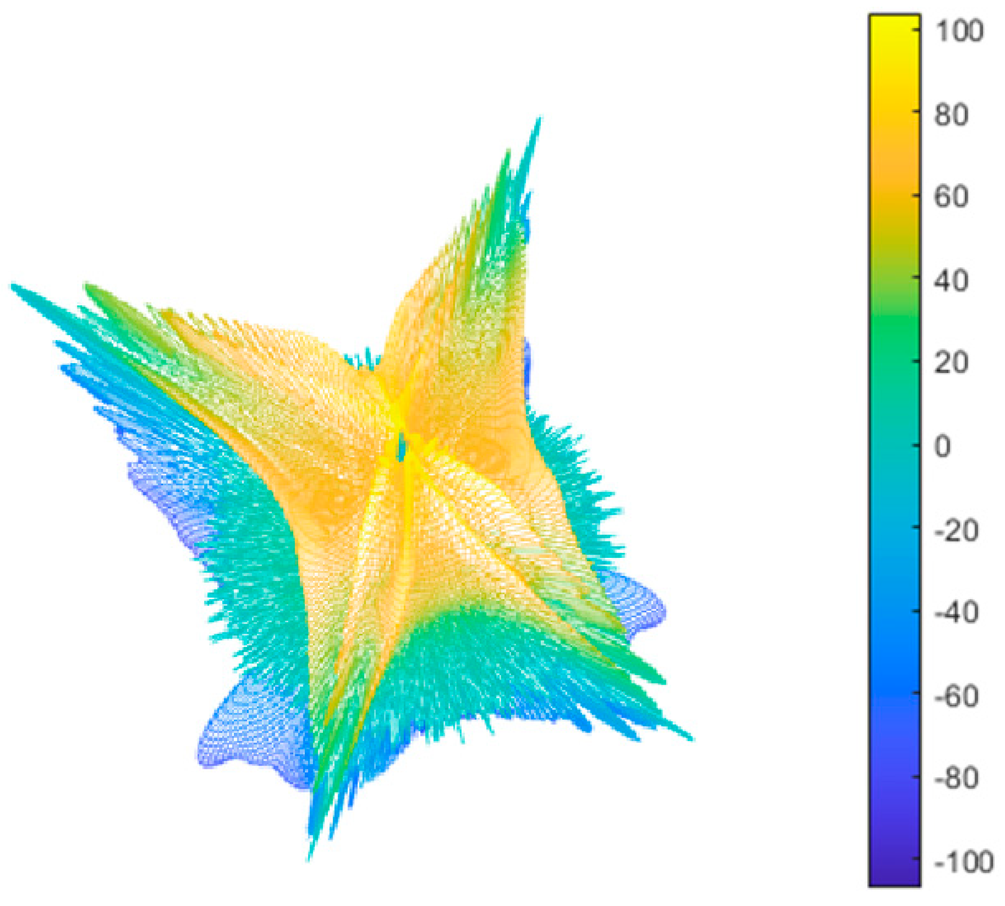
Lu et al. [7] proposed the turning-maneuver penetration method. In that paper, it was concluded that in a two-dimensional environment, the RCS peak exposure time could be significantly reduced by applying this method. However, in a three-dimensional scene, the RCS peaks are not confined only to the azimuth angle domain, but also extend into the elevation angle domain, as depicted in Figure 1.

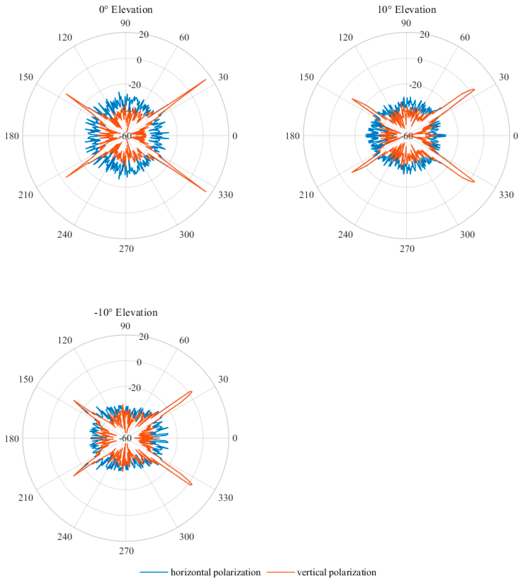
As shown in Figure 1, to draw the RCS in different azimuth and elevation angle, the RCS in dBsm has been added a fixed value 50 to make sure all RCS value is positive, and the different colors shows different value of Z-axis. The azimuth domain has four peaks, and simultaneously, its RCS increases with the increase in the elevation angle, reaching peaks at both its apex and nadir. To observe this more clearly, the RCS variations with changes in the azimuth angle under different elevation angles are shown in Figure 2, and the RCS variations with changes in the elevation angle under different azimuth angles are displayed in Figure 3.

From Figure 2, it can be observed that there are two pairs of symmetric azimuth-related peaks, with corresponding peak exposure angles at 35° and 145°. Figure 3 illustrates the variations in RCS with elevation angle changes. From Figure 3a,b, under non-peak exposure azimuth angles, the RCS sharply increases as the elevation angle increases. Figure 3c demonstrates that even at peak exposure azimuth angles, the rise in RCS caused by an increase in the elevation angle is comparable to peak exposure.

According to the analysis above, it is evident that considering changes in the elevation angle is necessary in a 3D scenario.

2.2. Aerodynamic Model

The simplified aerodynamic model is used to describe the relationship of the angle of attack, flight speed, lift coefficient, and drag coefficient. The aerodynamic model describes how the aerodynamic forces on an aircraft change with flight speed. Using data calculated with Datcom for the aircraft, this study performs linear and quadratic fittings to examine the relationships between important aerodynamic coefficients at different Mach numbers. The lift coefficient is linearly related to the angle of attack, while the drag coefficient is modeled as a quadratic function of the lift coefficient. The formulas for these relationships are presented as follows:

$$\begin{gathered} C_L=k_{L1}\alpha +k_{L0} \\ {C}_D=k_{D2}{C}_L^2+k_{D1}{C}_L+k_{D0} \end{gathered}$$

(1)

It can be seen that the parameters $k_{L1}$, $k_{L0}$, $k_{D2}$, $k_{D1}$ and $k_{D0}$ can be interpolated given the Mach number. Therefore, $C_L$ and $C_D$ can be expressed as $C_L\left(\alpha \right)$ and $C_D\left(\alpha \right)$. The lift and drag coefficient curves are shown in Figure 4.

2.3. Engine Model

Engine data are obtained through calculations using the engine simulation software named EngineSim (https://www1.grc.nasa.gov/beginners-guide-to-aeronautics/enginesimu/, accessed on 1 January 2024), which was produced by NASA and includes thrust generation and fuel consumption. An interpolation model is developed based on the engine data, which integrates the flight altitude, Mach number, thrust, and fuel consumption rate. Utilizing this model, fuel consumption can be accurately calculated at each waypoint according to the corresponding values of flight altitude, Mach number, and thrust.

3. Analysis of the Turning Maneuver in the 3D Scene

The 3D-SASLRM method proposed by Guan et al. [6] describes a search approach for flight polyline trajectory planning; however, it does not consider the roll angle generated by the turning maneuver between two polyline segments, resulting in a neglect of the effects caused by changes in the elevation angle.

This section explores the influence of the turning angle, rolling angle, flight Mach number, and radar power factor on the detection probability during maneuver turns.

3.1. Influence of Turning Angle on Detection Probability

3.1.1. Distance of Radar D = 20 km

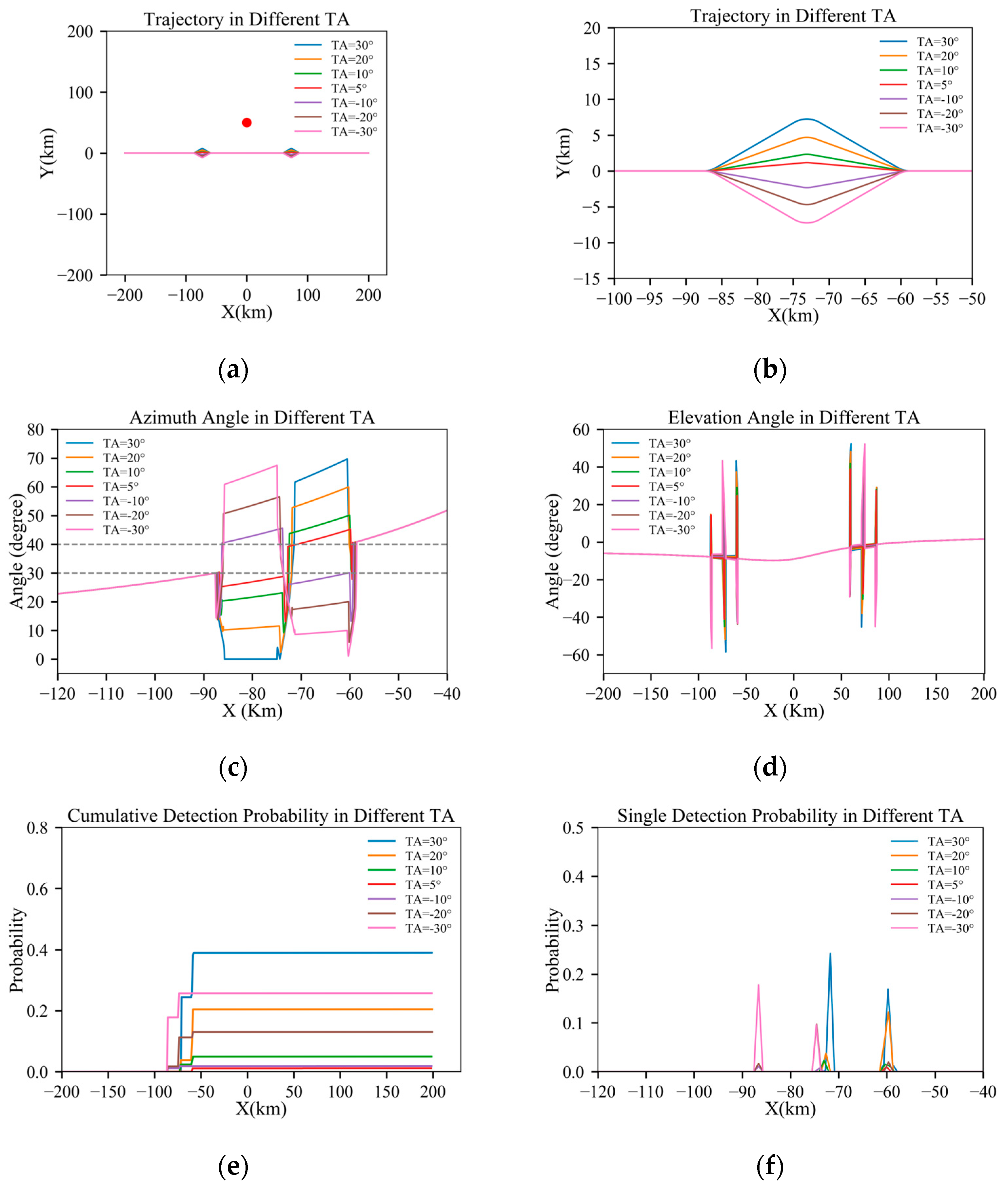
The trajectory configuration is shown in Figure 5a,b, where the red dot represents radar. The probabilities of detection for aircraft at turning angles (TA) of $30°, 20°, 10°, 5°,-10°,-20°$, and $-30°$ are compared, with other parameters set as outlined in

Table 1. Scene parameter settings in different TAs when D = 20 km.

Phi	Ma	$\mathit{D}$	Power Factor
60°	0.8	20 km	$1\times {10}^{-4}$

.

The parameter Phi is the rolling angle of the maneuver turn, and Ma is the flight Mach number. The radar distance is denoted by D, which means the y-coordinate of the radar. The power factor of the radar is $1\times {10}^{-4}$. The trajectory configuration, flight parameters, and detection probability results are shown in Figure 5.

Figure 5 illustrates the changes in the azimuth angle, elevation angle, cumulative detection probability, and single-detection probability of an aircraft at different turning angles during flight. The results show that the lowest probability of detection occurs at a turning angle of 5°. In contrast, when the turning angle increases to 10° and 20°, the peak single-detection probabilities significantly increase due to a rise in the elevation angle and closer proximity to the radar, leading to a substantial surge in the cumulative detection probability. Notably, the highest detection probability is observed when the turning angle is −30°, and when the aircraft turns upward or downward at the same angle, the detection probabilities are similarly close.

It is important to note that even when the turning angle is negative, increasing the distance from the radar, the larger pitch angles still lead to higher detection probability peaks. Analysis of changes in azimuth angle during the turn shows an increase in peak exposure times, further elevating the likelihood of the aircraft being detected.

Integrating these analyses, the changes in elevation angle significantly influence the aircraft’s detection probability in this scenario. Therefore, in designing flight trajectories and strategies, carefully controlling the turning and elevation angles is one of the keys to reducing the aircraft’s probability of detection.

3.1.2. Distance of Radar D = 50 km

The trajectory configuration is shown in Figure 6a,b, where the red dot represents radar. The probabilities of detection for aircraft at turning angles (TA) of $30°, 20°, 10°, 5°,-10°,-20°$, and $-30°$ are compared, with other parameters set as outlined in

Table 2. Scene parameter settings in different TAs when D = 50 km.

Phi	Ma	$\mathit{D}$	Power Factor
60°	0.8	50 km	$1\times {10}^{-4}$

.

Figure 6 displays the changes in the azimuth angle, elevation angle, cumulative detection probability, and single-detection probability of an aircraft at different turning angles during flight. Compared to a radar distance of 20 km, the hazardous area along the trajectory significantly expands at 50 km, necessitating a larger turning range to evade radar detection. Figure 6e shows that the lowest probability of detection occurs at a turning angle of 5°, indicating the most effective penetration at this angle. Moreover, the difference in detection probability between this and a turning angle of −10° is relatively small.

3.1.3. Distance of Radar D = 100 km

The trajectory configuration is shown in Figure 7a,b, where the red dot represents radar. The probabilities of detection for aircraft at turning angles (TA) of $30°, 20°, 10°, 5°,-10°,-20°$, and $-30°$ are compared, with other parameters set as outlined in

Table 3. Scene parameter settings in different TAs when D = 100 km.

Phi	Ma	$\mathit{D}$	Power Factor
60°	0.8	100 km	$1\times {10}^{-4}$

.

Figure 7 shows the variations in an aircraft’s azimuth angle, elevation angle, cumulative detection probability, and single-detection probability at different turning angles during flight. According to Figure 7e, the lowest probability of detection also occurs at a turning angle of 5°, which is almost zero.

3.1.4. Analysis

A comprehensive analysis under the conditions of radar distances of 20 km, 50 km, and 100 km reveals that the required range of turning fluctuations increases with the increase in radar distance D. However, at a turning angle TA of 5°, due to the relatively small changes in the pitch angle, this angle consistently demonstrates the most effective penetration performance. This indicates that, in this scenario, maintaining minimal changes in pitch angle is a key factor in reducing the probability of detection.

3.2. Influence of Rolling Angle on Detection Probability

3.2.1. TA = 5°, D = 20 km

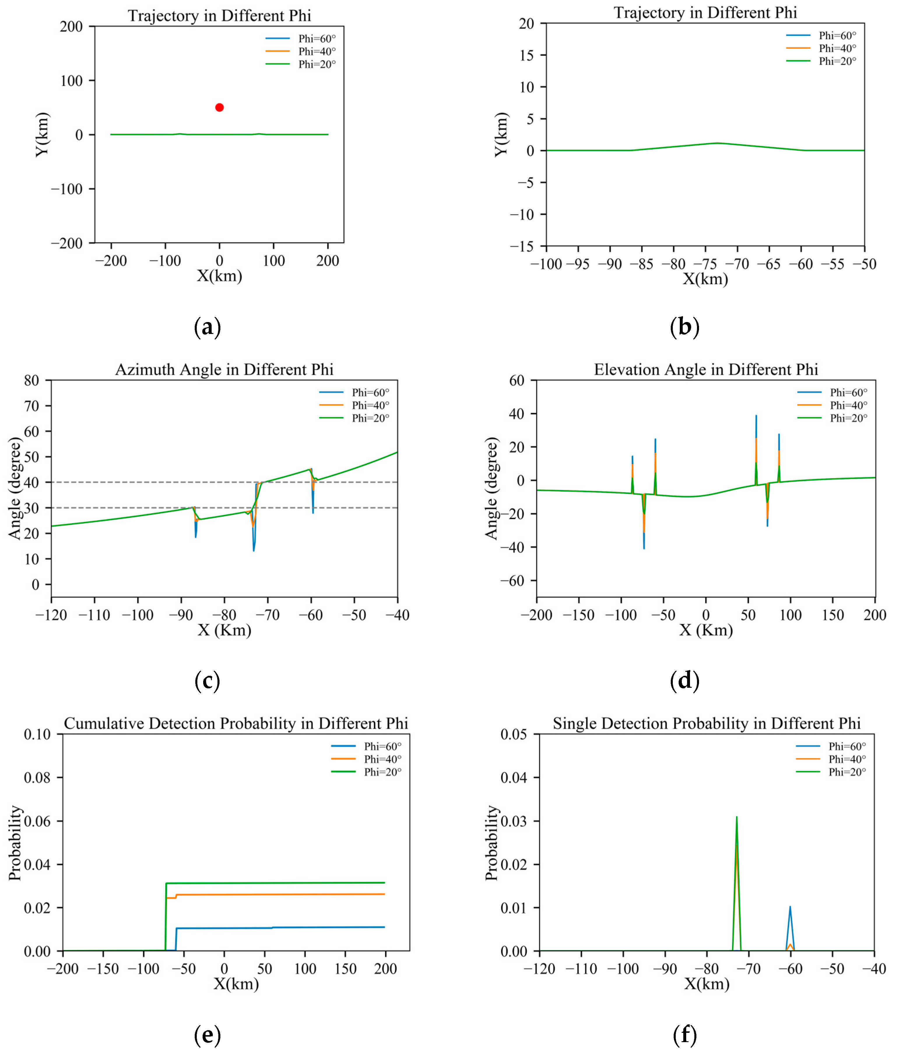
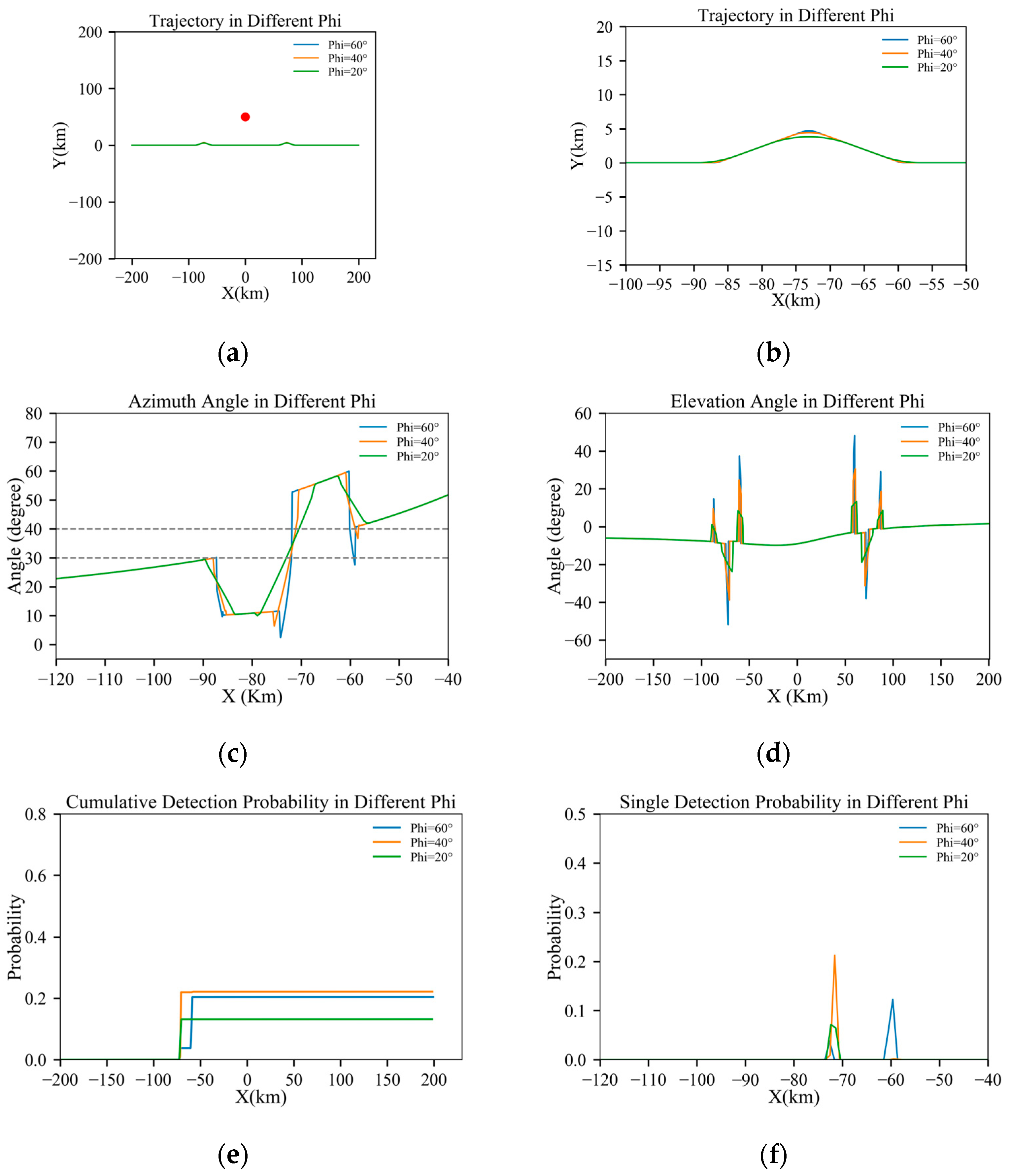
The trajectory configuration is shown in Figure 8a,b, where the red dot represents radar. The probabilities of detection for aircraft at rolling angles of 60°, 40°, and 20° are compared, with other parameters set as indicated in

Table 4. Scene parameter settings in different rolling angles when TA = 5° and D = 20 km.

TA	Ma	$\mathit{D}$	Power Factor
5°	0.8	20 km	$1\times {10}^{-4}$

.

Figure 8 illustrates the influence of the aircraft rolling angle on detection probability, considering the variations in the azimuth angle, elevation angle, cumulative detection probability, and single-detection probability during the flight with rolling angles of 20°, 40°, and 60° at a turning angle of 5°. The results indicate that at a rolling angle of 60°, the aircraft’s peak detection probability is relatively low, and the cumulative detection probability is the smallest. The azimuth graph, Figure 8c, shows that at a high rolling angle, the aircraft spends less cumulative time in the hazardous azimuth angle regions during turns and has fewer exposures, thereby reducing the cumulative detection probability along the entire trajectory.

3.2.2. TA = 5°, D = 50 km

The trajectory configuration is shown in Figure 9a,b, where the red dot represents radar. The probabilities of detection for aircraft at rolling angles of 60°, 40°, and 20° are compared, with other parameters set as indicated in

Table 5. Scene parameter settings in different rolling angles when TA = 5° and D = 50 km.

TA	Ma	$\mathit{D}$	Power Factor
5°	0.8	50 km	$1\times {10}^{-4}$

.

Figure 9 depicts the changes in the azimuth angle, elevation angle, cumulative detection probability, and single-detection probability of an aircraft at a turning angle of 5° and a radar distance D of 50 km, with rolling angles of 20°, 40°, and 60°. Similar to the scenario with a radar distance D of 20 km, the aircraft’s detection probability is lowest at a 60° rolling angle and highest at a 20° rolling angle.

3.2.3. TA = 20°, D = 50 km

Figure 10a,b shows the trajectory configuration, where the red dot represents radar. The probabilities of detection for aircraft at rolling angles of 60°, 40°, and 20° are compared, and other parameters are set as indicated in

Table 6. Scene parameter settings in different rolling angles when TA = 20° and D = 50 km.

TA	Ma	$\mathit{D}$	Power Factor
20°	0.8	50 km	$1\times {10}^{-4}$

.

Figure 10 illustrates the variations in the azimuth angle, elevation angle, cumulative detection probability, and single-detection probability of an aircraft at a turning angle of 20° and a radar distance D of 50 km, with rolling angles of 20°, 40°, and 60°. From 3.2.2, at a turning angle of 5° and a rolling angle of 60°, the aircraft’s detection probability peak is relatively low, and its cumulative detection probability is the smallest. According to Figure 10f, when the turning angle increases to 20°, it shows that, although a larger turning speed is achieved with a high rolling angle, it results in more exposures at hazardous azimuth angles under large turning angles, thereby increasing the cumulative detection probability along the entire trajectory. In this scenario, a 20° rolling angle performs the best.

3.3. Influence of Flight Speed on Detection Probability

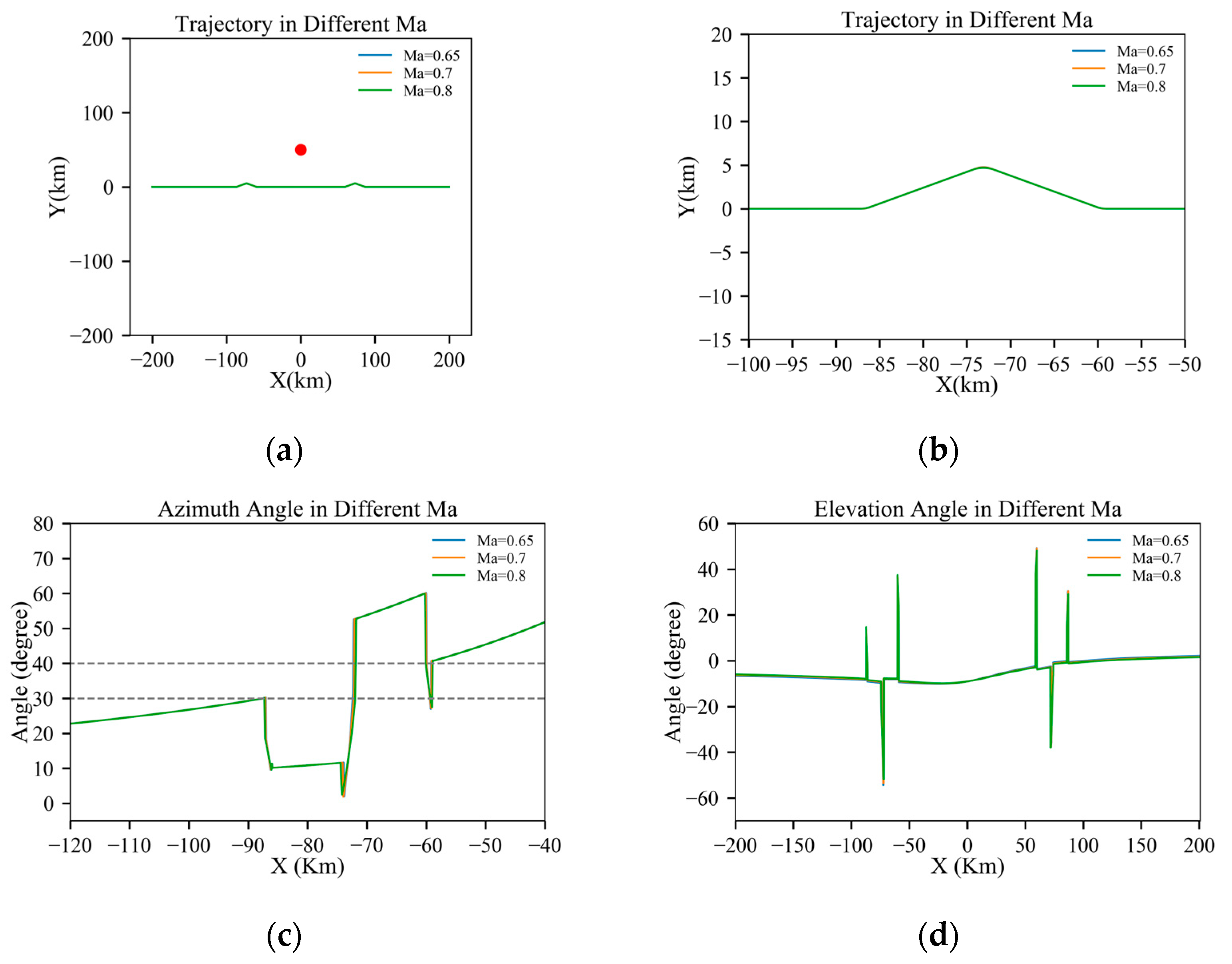
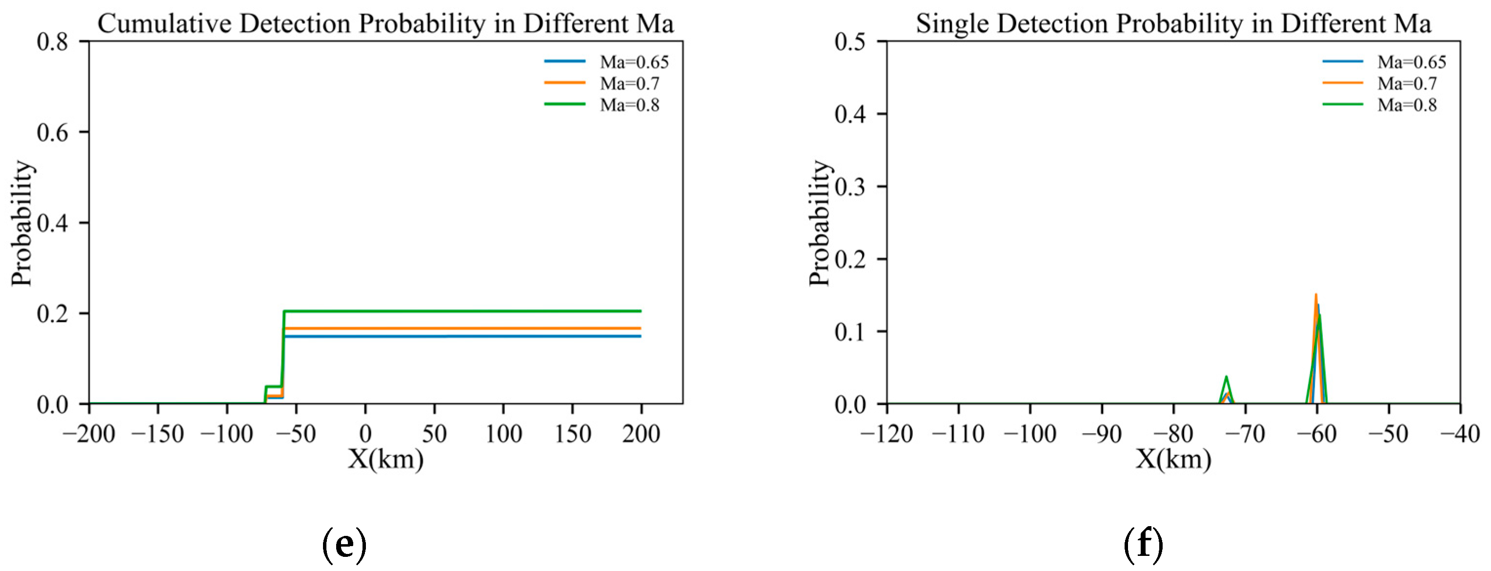
The trajectory configuration is shown in Figure 11a,b, where the red dot represents radar. The probability of detection for aircraft at Mach numbers of 0.65 and 0.7 are compared, and other parameters are set as indicated in

Table 7. Scene parameter settings in different flight speeds.

TA	Phi	$\mathit{D}$	Power Factor
20°	60°	50 km	$1\times {10}^{-4}$

.

Figure 11 displays the variations in the azimuth angle, elevation angle, cumulative detection probability, and single-detection probability of an aircraft flying at Mach numbers of 0.65, 0.7, and 0.8. It is evident that the Mach number has a significant influence on the peak values of single-detection probability, leading to differences in cumulative detection probability. Contrary to conclusions drawn in two-dimensional scenarios, the lowest detection probability in this scenario occurs at Ma = 0.65. This phenomenon can be attributed to higher speed, causing more turning time and more time during which the high-elevation angles’ exposure to the radar increases, leading to an increase in RCS peak exposure time. This suggests that an analysis of elevation angles in three-dimensional scenarios is necessary. Although variations in flight speed do affect radar detection probabilities, their overall influence is relatively limited.

3.4. Influence of Radar Power Factor on Detection Probability

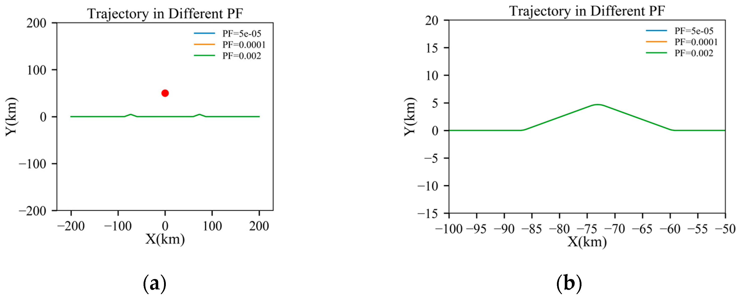
The trajectory configuration is shown in Figure 12a,b, where the red dot represents radar. The probabilities of detection for aircraft at radar power factors of $5\times {10}^{-5}$, $1\times {10}^{-4}$, $2\times {10}^{-3}$ are compared, with other parameters set as indicated in

Table 8. Scene parameter settings in different power factors.

TA	Phi	$\mathit{D}$	Ma
20°	60°	50 km	0.8

.

Figure 12 shows changes in the azimuth angle, elevation angle, cumulative detection probability, and single-detection probability of an aircraft under radar power factors of $5\times {10}^{-5}$, $1\times {10}^{-4}$, $2\times {10}^{-3}$ The analysis reveals that radar power factors primarily increase the cumulative detection probability by enhancing the peak values of single-detection probabilities while having minimal influence on other flight parameters, such as the azimuth and elevation angle. Therefore, although radar power factors can influence the probability of detection, their practical value is relatively limited when formulating trajectory planning and tactical decisions during aircraft penetration operations.

3.5. Scenario with Two Radars

3.5.1. Influence of Turning Angle in a Scenario with Opposing Dual Radars

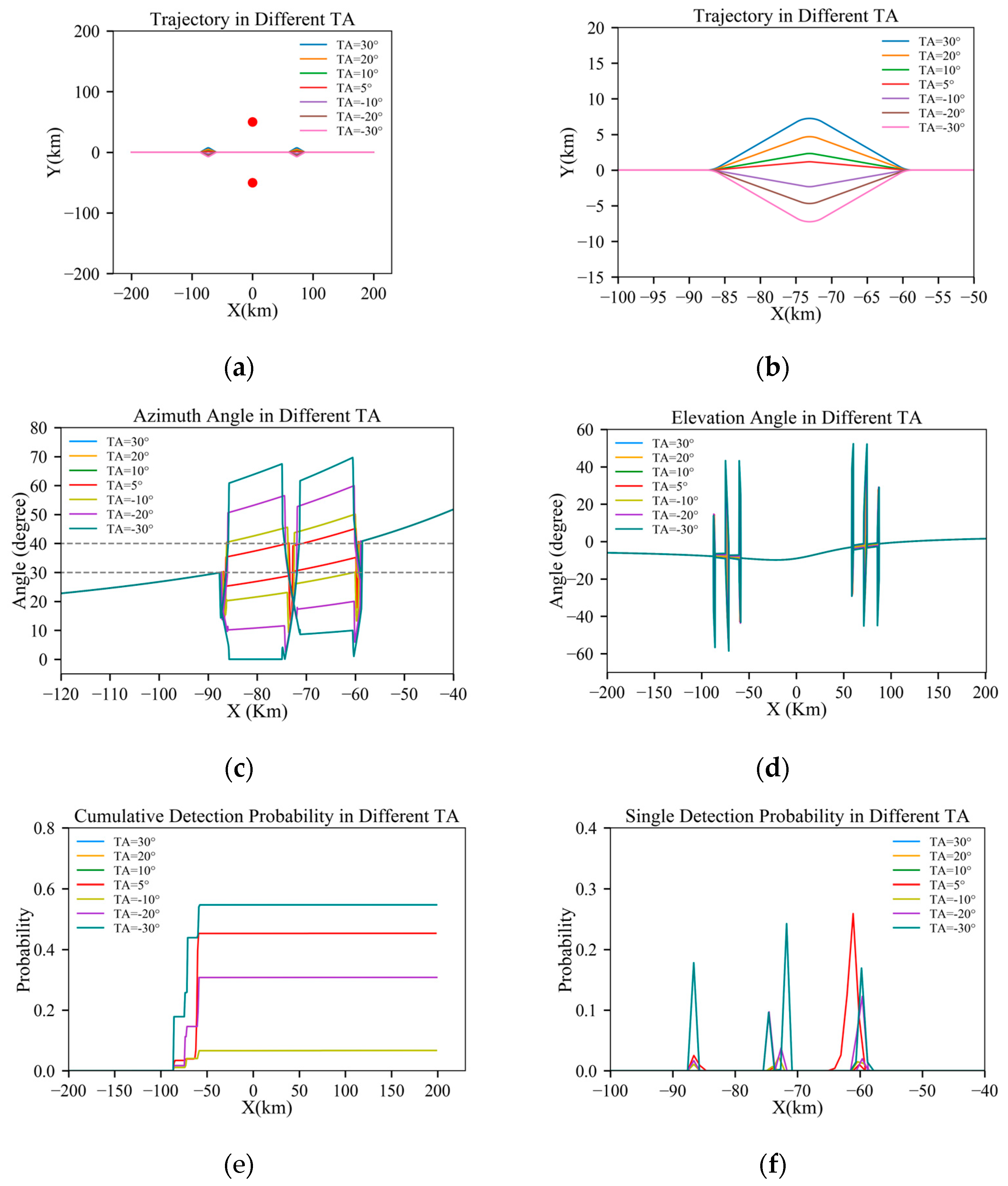
Figure 13 displays the changes in flight parameters for an aircraft performing penetration maneuvers at turning angles of 30°, 20°, 10°, 5°, −10°, −20°, and −30° in a scenario with opposing dual radars. Other parameter settings are as specified in

Table 9. Scene parameter settings in a scenario with dual radars.

Power Factor	Phi	$\mathit{D}$	Ma
$1\times {10}^{-4}$	60°	50 km	0.8

. And the red dots in Figure 13a represent radars.

Figure 13 shows the changes in the azimuth angle, elevation angle, cumulative detection probability, and single-detection probability of an aircraft at different turning angles in a scenario with opposing dual radars. It illustrates that a 5° turning angle is no longer optimal when radars are on both sides. This is because, although the aircraft evades the hazardous azimuth angles of the radar on one side by turning, it enters directly into the high detection probability area of the opposite-side radar upon realigning, leading to peak exposure and a significant increase in the cumulative detection probability. At this point, ±10° becomes the best choice in this scenario, serving as a strategy to balance the avoidance of a threat on one side while reducing exposure on the other. Consistent with the analysis in 3.1 of the turning angles, the detection probability is highest at ±30° turning angles.

3.5.2. Influence of Turning Angle in a Scenario with a Closely Positioned Radar

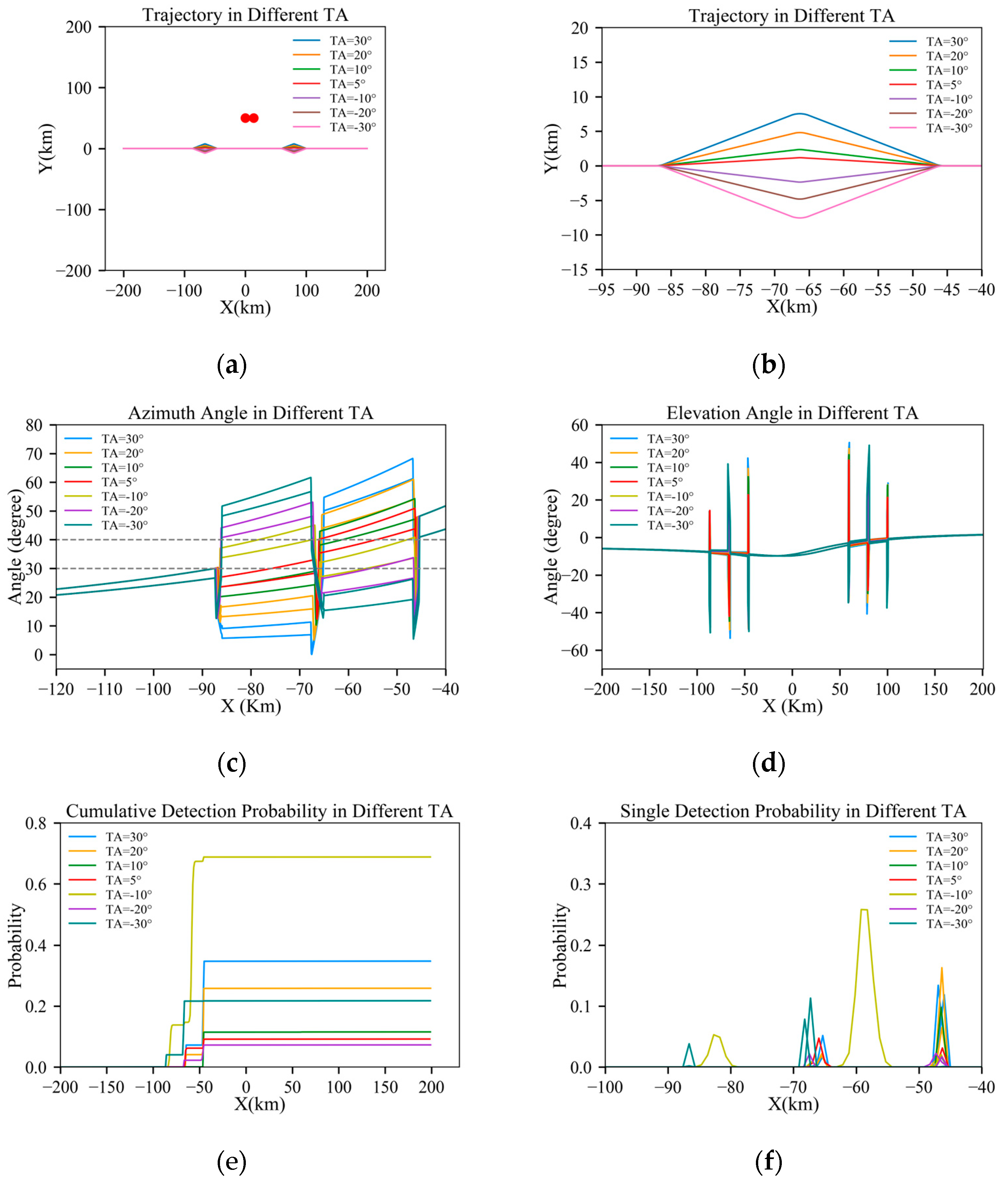
Figure 14 displays the changes in flight parameters for an aircraft performing penetration maneuvers at turning angles of 30°, 20°, 10°, 5°, −10°, −20°, and −30° in a scenario with a closely positioned radar on the same side. In this situation, the aircraft makes a turn while simultaneously crossing the hazardous areas of both radars. Other parameter settings are the same as in Table 9. And the red dots in Figure 14a represent radars.

Figure 14 shows the changes in the azimuth angle, elevation angle, cumulative detection probability, and single-detection probability of an aircraft at different turning angles in a scenario with closely positioned dual radars on the same side. From this, it can be seen that when two radars are nearby, if the aircraft adopts a single-turn maneuver to evade the hazardous areas of both radars simultaneously, the lowest detection probability occurs at a −20° turning angle, a slightly higher detection probability at a 5° turning angle, and the highest detection probability at a −10° turning angle due to exposure to high-intensity peak detection zones.

3.5.3. Influence of the Turning Angle in a Scenario with Radars Positioned Further Apart

Figure 15 displays the changes in flight parameters for an aircraft performing penetration maneuvers at turning angles of 30°, 20°, 10°, 5°, −10°, −20°, and −30° in a scenario with radars positioned further apart on the same side. In this situation, the aircraft makes two turns while simultaneously crossing the hazardous areas of the radars. Other parameter settings are the same as in Table 9. And the red dots in Figure 15a represent radars.

Figure 15 shows the changes in the azimuth angle, elevation angle, cumulative detection probability, and single-detection probability during the flight of an aircraft at different turning angles in a dual radar scenario on the same side and at a longer distance. It can be seen that when the turning angle is 5°, the aircraft has the lowest probability of detection. This is mainly because the aircraft maintains a small elevation angle at this turning angle. Hence, the peak value of the single-detection probability is small, resulting in a relatively low cumulative detection probability. Conversely, when the turning angle is −20°, there is the highest probability of detection due to the prolonged and intense peak exposure to which the aircraft has been subjected. It shows that the choice of the turning angle has an important effect on reducing radar detection probability when planning flight trajectories and penetration strategies.

3.6. Summary

This section investigates the influence of various factors, including the turning angle, rolling angle, flight speed, and radar power factor, on radar detection probability in both single-radar and dual-radar scenarios. The results indicate that during the process of an aircraft avoiding the hazardous areas of radar detection, optimizing the aircraft’s turning angle and rolling angle can effectively reduce its exposure time, thereby significantly lowering the overall probability of detection.

Results reveal that the turning angle is particularly critical among the factors examined. In a single-radar scenario, a 5° turning angle has been found to yield optimal performance during the aircraft’s penetration process. Regarding the aircraft’s flight speed, the study demonstrates that the radar detection probability is lower at a Mach number (Ma) of 0.65 than at Ma = 0.8. It is hypothesized that this discrepancy is due to the increase in turning maneuver time, leading to an increase in the RCS peak exposure time. This finding contradicts the conclusions drawn from two-dimensional scenarios, highlighting the necessity of analyzing elevation angles in 3D scenarios. Additionally, the analysis of various rolling angles suggests that when the adverse effects of a significant elevation angle increase, induced by high overload, they outweigh the time accumulation benefits, and that employing high overload is no longer the optimal strategy for executing penetration maneuvers.

These conclusions provide significant guidance for subsequent flight trajectory planning and tactical decision making, emphasizing the necessity for precise maneuvering in complex environments.

4. RVR-TM Algorithm

4.1. Analysis of the Turning Maneuver

However, in the 3D scene, the elevation angle rapidly increases during the turning maneuver, which can cause an increase in detection probabilities. Thus, we need to analyze the factors that influence turning maneuvers.

During the maneuver, the radius is the function of load factor N.

$$R=\frac{V^2}{\sqrt{N^2-1}g}$$

(2)

In Formula (2), $R$ is the turning radius, $V$ is the turning velocity, $N$ is the load factor, and $g$ is the gravitational acceleration. Thus, the turning time can be as follows:

$$T=\frac{\theta R}{V}=\frac{\theta V}{\sqrt{N^2-1}g}$$

(3)

In Formula (3), T is the turning time, and $\theta$ is the turning angle. According to Formula (2), the turning time is proportional to the turning angle and velocity. Thus, a decrease in turning velocity can reduce the RCS peak exposure time and the detection probability, which is counterintuitive.

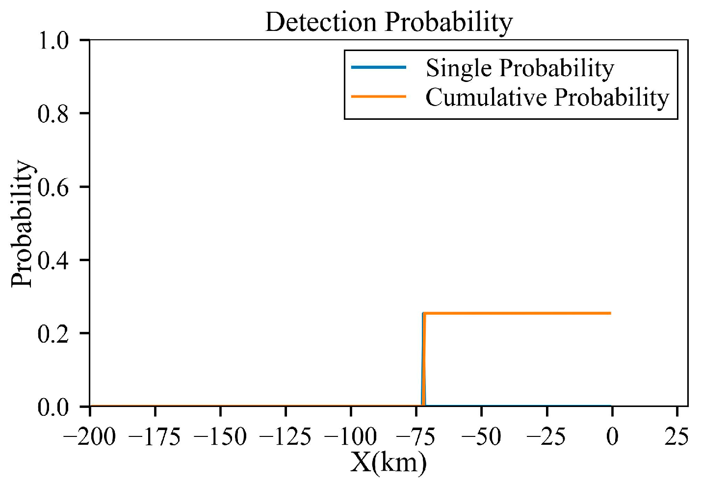
Based on this conclusion, we can propose a new turning-over method with the lowest turning angle and velocity, as shown in Figure 16. The detection probabilities are shown in Figure 17. The azimuth and elevation angle curves are shown in Figure 18.

4.2. Steps of the RVR-TM Algorithm

The steps of the RVR-TM algorithm are given as shown in Algorithm 1.

Algorithm 1 The RVR-TM algorithm

Input: Coordinates of the start node $P_s$, coordinates of the goal node $P_g$, radar layout.

Output: Trajectory.

1: while not reach goal node do

2: if ($Distance to Radar\le 2 \ast Radar Valley Radius$) then

3:    Hover around Radar;

4:    return New Command;

5:    Continue;

6: if ($Distance to Radar\le 2 \ast Radar Valley Radius$) then

7:    Do Turning Maneuver;

8:    return New Command;

9:    Continue;

10: else then

11:  return NONE;

12:  Continue;

4.3. Simulations in Single-Radar Scenario

The radar specification parameters used in the simulation are shown in

Table 10. Radar parameters for single-radar threat environment for RVR-TM algorithm.

Index	${\mathit{T}}_{\mathit{s}\mathit{c}\mathit{a}\mathit{n}}$ (s)	${\mathit{P}}_{\mathit{F}\mathit{A}}$	N	$\mathit{\rho }$	${\mathit{V}}_{\mathit{H}}$	${\mathit{R}}_{\mathit{H}}$	Power Factor
1	4	$1\times {10}^{-6}$	2	0.5	0	0	$1\times {10}^{-4}$

.

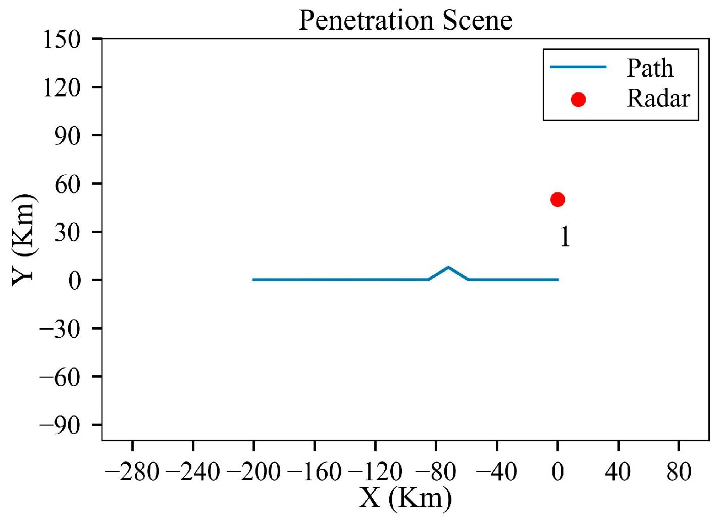
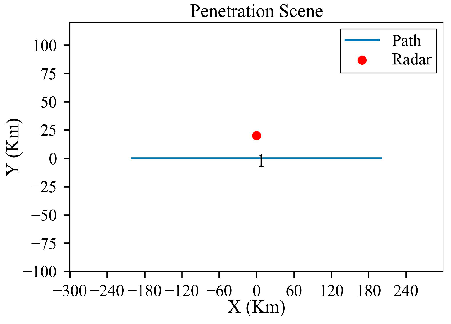
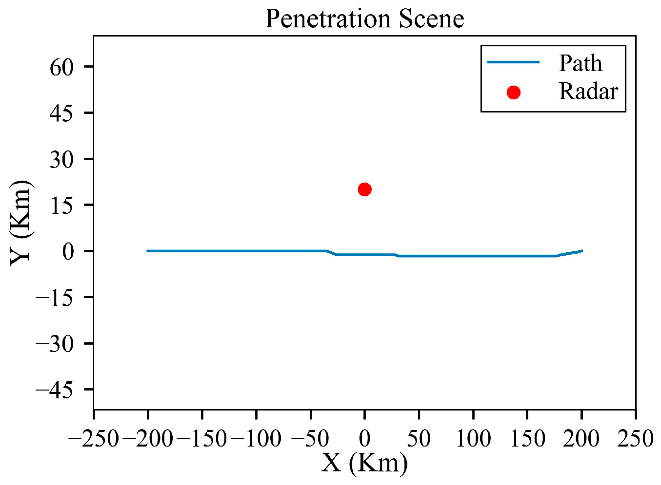
The analysis environment is shown in Figure 19; the mission is defined as a penetration from (−200, 0, 8) to (200, 0, 8), and the radar is located at (0, 20, 0) with normal power.

4.3.1. Straight Trajectory

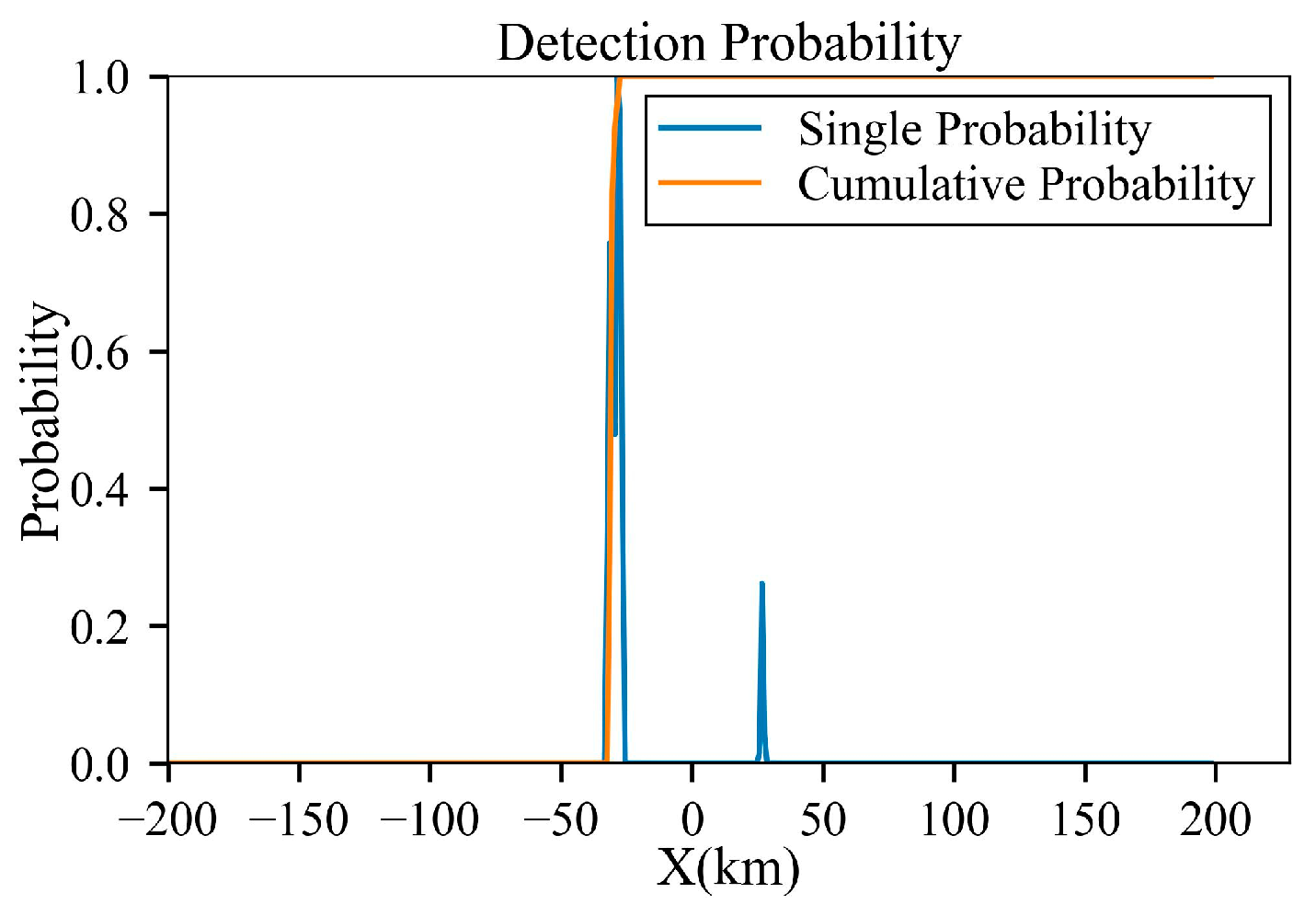
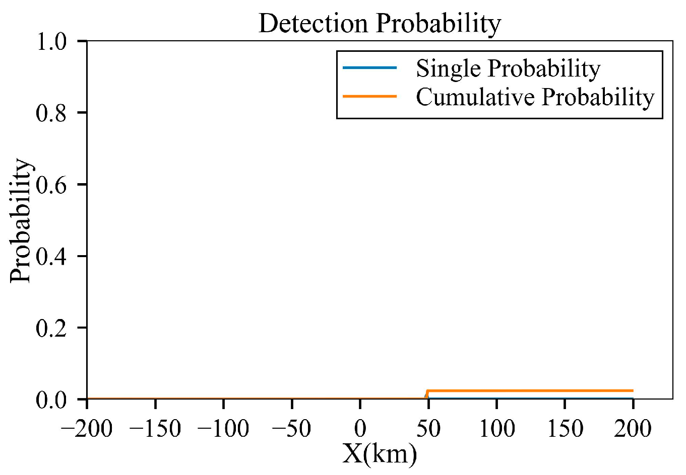
Figure 20 and Figure 21 reveal that during the aircraft’s flight, the RCS peaks at 35 degrees forward-left and 145 degrees backward-left are exposed to the radar for extended periods, leading to the aircraft’s detection. Concurrently, as the aircraft approaches the (0,0) point, its elevation angle, relative to the radar, increases. However, due to the maximal value of the elevation angle not being significantly large, this does not manifest as a pronounced peak on the detection probability curve.

4.3.2. RVR-TM Method

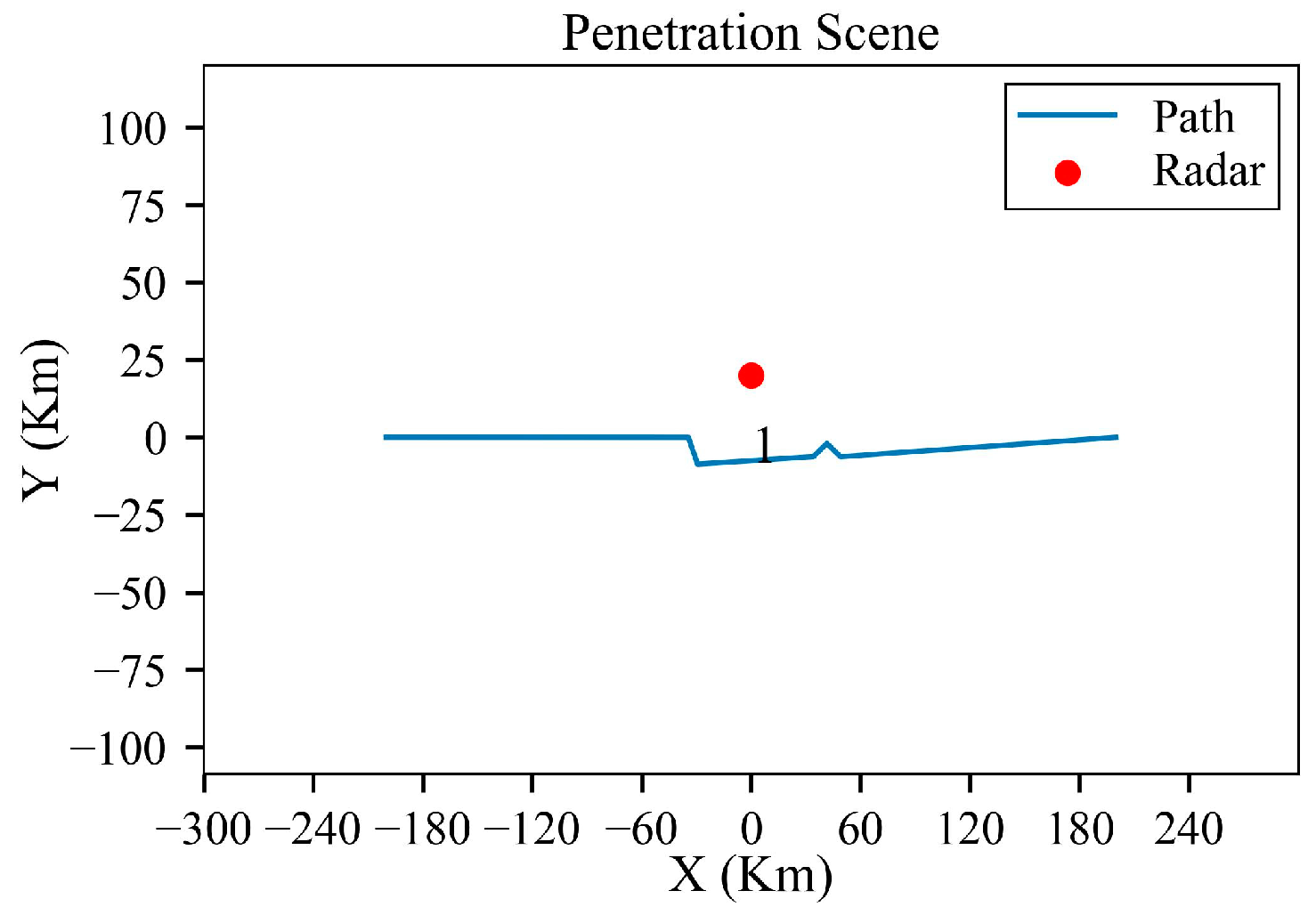
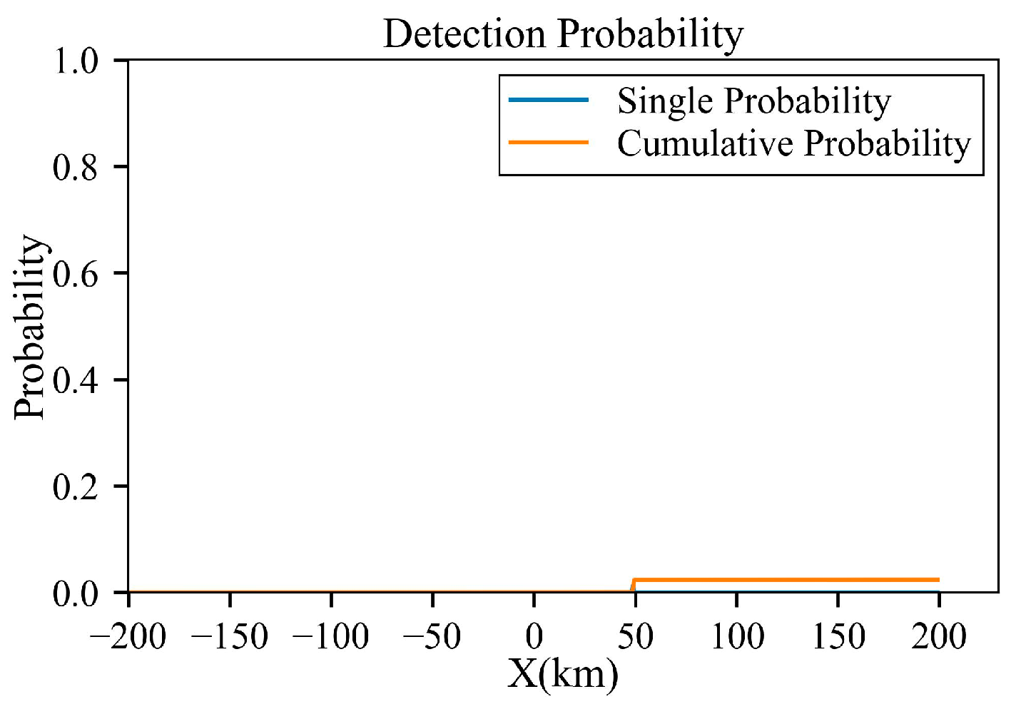
From Figure 22, Figure 23 and Figure 24, it is observed that during the aircraft’s penetration process, it first encounters the radar valley radius range, thereby moving perpendicularly to the radar valley radius to avoid entering the hazardous zone. Upon exiting the radar valley radius area, it continues to advance toward the target point. Near (50,0), to prevent the aircraft’s rear-left RCS peak from being exposed to the radar for an extended duration, the aircraft executes a maneuvering turn, allowing the RCS peak to swiftly sweep past the radar station, ultimately reducing the overall trajectory radar detection probability from 100% to 2%. The total Planning Time is 8.18 s.

4.3.3. D-SASLRM Method

Figure 25 and Figure 26 illustrate that the 3D-SASLRM method can produce a planned trajectory with a minimal radar detection probability (0.1%), albeit at the cost of a longer search duration, which amounts to 126.72 s.

4.4. Simulations in a Three-Radar Scenario

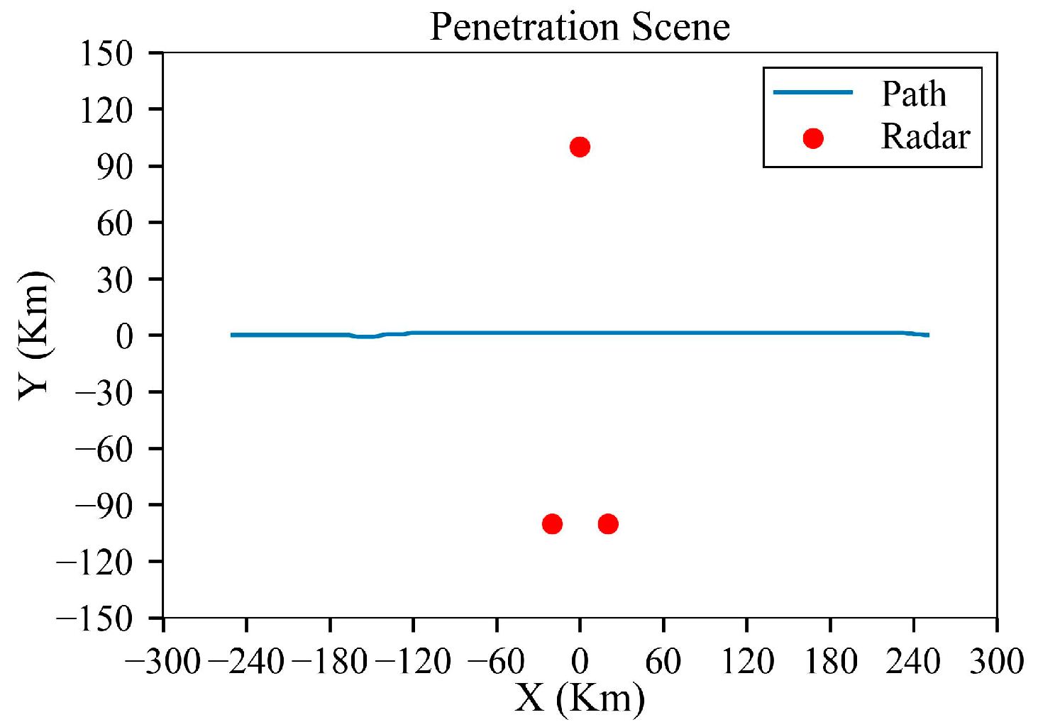
The radar parameters are set in Table 10. The analysis environment is shown in Figure 27. The mission is defined as a penetration from (−250, 0, 8) to (250, 0, 8), and the radar is located at (0, 100, 0), (−20, −100, 0), or (20, −100, 0) with normal power.

4.4.1. Straight Trajectory

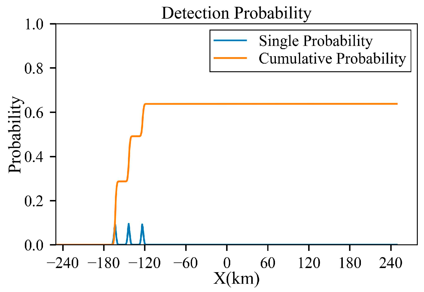
Figure 28 and Figure 29 reveal that during the aircraft’s flight, the RCS peaks at 35 degrees forward-left and 145 degrees backward-left are exposed to the radar for extended periods, leading to the aircraft’s detection. Concurrently, as the aircraft approaches the (0,0) point, its elevation angle relative to the radar increases. However, due to the maximal value of the elevation angle not being significantly large, this does not manifest as a pronounced peak on the detection probability curve.

4.4.2. RVR-TM Method

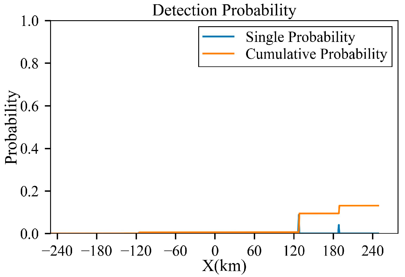
From Figure 30, Figure 31 and Figure 32, it is observed that during the aircraft’s penetration process, it ultimately reduces the overall trajectory radar detection probability from 64% to 12%. The total Planning Time is 75.89 s.

4.4.3. D-SASLRM Method

Figure 33 and Figure 34 illustrate that the 3D-SASLRM method can produce a planned trajectory with a minimal radar detection probability (0.6%), albeit at the cost of a longer search duration, which amounts to 330.43 s.

5. Reinforcement Learning Algorithm

Based on Section 3 and Section 4, reinforcement learning is applied to intelligent decision-making regarding stealth aircraft penetration.

Proximal Policy Optimization (PPO) is a reinforcement learning algorithm that utilizes stochastic policy gradients, applicable to both continuous and discrete action spaces. The PPO algorithm is based on the Actor-Critic framework, which includes two Actor networks and one Critic network. This structure employs an online policy during training, meaning the policy used for generating samples is the same as that used for training.

The main innovation of PPO lies in its solution to the issue of step-size selection in policy gradient algorithms. It introduces a mechanism to limit the magnitude of policy updates, thereby maintaining the stability of the training process. This approach not only stabilizes the training process but is also widely appreciated for its simplicity of implementation, ease of tuning, and excellent performance. Currently, PPO has become one of the commonly used reinforcement learning algorithms by OpenAI. These features have made PPO perform exceptionally well in various tasks and environments, especially in scenarios that require handling complex action spaces.

5.1. Reinforcement Learning Decision Process

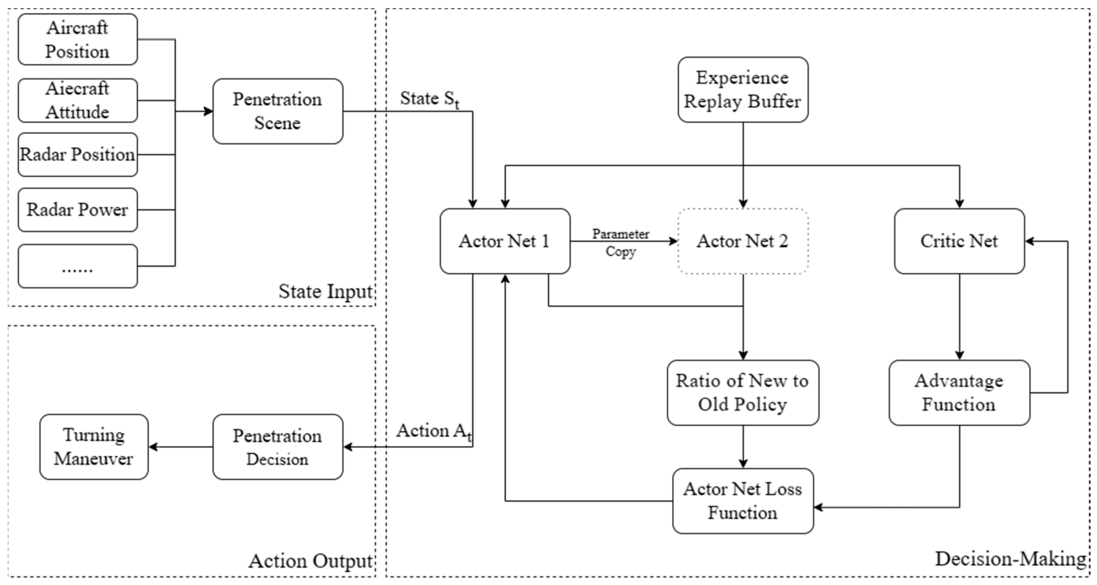
Based on the PPO algorithm and drawing on the relevant conclusions from the simulations discussed earlier in the text, this paper has established a decision-making model for the penetration of stealth aircraft. The decision-making model for stealth aircraft penetration is designed as an integrated system, with the aim of achieving efficient penetration operations without detection by enemy radar systems. The decision-making model comprises three main components, namely, a state input module, a decision-making module, and an action output module, as shown in Figure 35.

The state input module is responsible for collecting key information from multiple sources, such as the aircraft’s current velocity, position, attitude, and radar detection information. These data points are aggregated into a state vector, which provides the necessary contextual information for decision making.

The decision-making module is driven by the PPO reinforcement learning algorithm, which includes two key neural networks: the Actor and Critic networks. The Actor network is responsible for proposing actions, generating two sets of outputs by analyzing the state vector $S_t$, an exploratory action network (Actor network 1) and a deterministic action network (Actor network 2). Exploratory actions allow the aircraft to explore new penetration strategies during training, while deterministic actions execute the optimal behavior based on the trained model. In actual operation, there is no need to maintain two Actor networks simultaneously; instead, the norms of the two sets of networks are stored separately, updating the strategy by retaining some old policy samples for comparison with the new strategy. Consequently, the Actor network 2 in Figure 35 is indicated with a dashed frame to signify that it is not a physical entity. Meanwhile, the Critic network evaluates the performance of the current policy, providing feedback values (value function outputs) to help optimize the strategy generated by the Actor network.

Subsequently, based on the output of the Actor network, the action output module executes specific actions $A_t$. After the action is executed, the results of the aircraft’s interaction with the environment, including signals received from enemy radar, are collected and fed back into the experience pool.

In the experience pool, a large amount of data on aircraft states and action outcomes are stored, providing rich learning material for the decision-making module. Using this data, the model continuously improves its decision-making quality through iterative training, ensuring effective stealth penetration behavior in different penetration scenarios. In addition, the results of the action execution are used to adjust the model further to ensure that the aircraft’s penetration actions are both covert and effective.

Through this process of cyclical learning and adjustment, the stealth aircraft penetration decision-making model aims to achieve adaptive and optimized behavior in complex hostile environments, thereby increasing the success rate of the mission.

5.2. State Space Design

5.2.1. Deterministic Expression of Detection Probability

When training the penetration decision-making model for stealth aircraft, the Monte Carlo method is used to estimate the probability of the aircraft being detected by radar through random simulation. Although this method can theoretically simulate complex stochastic processes, it also introduces significant uncertainty into the training. Specifically, because the radar detection is stochastic, using the results of the Monte Carlo simulation as the basis for training can make the signals in the learning process extremely unstable.

To reduce this uncertainty and improve training efficiency, it is necessary to transform the random event of the aircraft detected by radar into a numerical expression. Since radar detection probabilities are usually represented in a multiplicative form (cumulative risk), applying them directly to the reward function complicates matters. In contrast, logarithmic transformation is an effective method that converts the multiplication of cumulative probabilities into addition, facilitating direct provision as rewards or penalties to the aircraft.

For this reason, in the penetration decision-making model constructed in this paper, the following deterministic expression method for detection probability is proposed:

Logarithmic Probability Transformation: By taking the logarithm of the radar detection probability, the product of cumulative probabilities is converted into a summation form, which allows for a more direct integration into the reward function;

Deterministic Mission Failure Condition: Instead of the random comparison method based on the Monte Carlo model, a clear maximum detection probability threshold can be set, such as 30%; when the cumulative logarithmic probability exceeds the corresponding logarithmic value, the mission is judged to have failed;

Logarithmic Transformation of Health and Damage Values: Combining the above two points, the health value of the aircraft is defined as the negative logarithm of the maximum allowable detection probability; for example, if the highest probability is 30%, then the health value is set to $-log\left(1-0.3\right)$; similarly, the radar detection probability increase caused by each danger point is also represented by the negative logarithm of the detection probability, converted into damage value.

Compared to the Monte Carlo method, the advantage of this state space design lies in transforming uncertainties and probabilistic issues into deterministic numerical problems, significantly enhancing the stability of the training process. This approach eliminates randomness in the training process, allowing the agent to learn effective penetration strategies within the radar coverage area more robustly, thereby improving the learning efficiency and policy performance of the entire model. Moreover, this method facilitates the agent’s ability to assess the potential risks of the actions, optimize the trajectory selection, and maximize mission success rates while minimizing the risk of being detected.

5.2.2. Dual-Layer State Space

In the construction of the stealth aircraft penetration decision-making model, this paper designs a dual-layer state space, which includes the external input state and the true state used for decision making. This design fully utilizes environmental information, transforming high-dimensional raw data into lower-dimensional data that are more direct and effective for decision making, thereby enhancing the learning efficiency and decision quality of the agent.

The external input state includes the initial position, velocity, and health value of the aircraft, as well as the positions of the radar and the target, etc., providing the absolute position of the aircraft in the environment. However, directly using these high-dimensional, absolute coordinate data may lead to the decision-making process of the agent being susceptible to overfitting, especially when the positions of the radar and the target are fixed and unchanged.

To address this issue, this paper introduces a true state space, which characterizes the positional relationship of the aircraft relative to the radar and the target based on relative azimuth angles and relative distances. The design of the true state space reflects a description based on the relative relationships between the agent and key environmental objects, rather than relying on a global coordinate system. This design helps the agent learn to make more adaptable decisions under varying environments.

During the training process, the true state, which changes with every movement of the aircraft, has a dynamic characteristic that not only prevents overfitting but also enriches the agent’s experience. It provides a more diverse range of scenarios to promote generalization learning. Since the true state no longer directly depends on unchanging references in the environment, such as specific landmarks or radar positions, the agent can learn effective decision making in various environments, rather than only performing well under particular conditions. At the same time, the agent does not need to relearn strategies when facing radars with different positions but essentially the same configuration, which enhances the model’s applicability and robustness in unknown environments.

The true state space plays a central role in the agent’s decision-making process, directly affecting the behavioral output of the Actor network and providing the Critic network with a basis for evaluating the quality of the strategy. This accelerates the learning process, especially in handling complex interactions and adapting quickly to environmental changes.

In summary, models that directly use the agent’s position, radar’s position, and target position as states are susceptible to the limitations of specific environmental settings. Compared to methods that directly construct a map, the true state space approximates the use of “relative azimuth angles are important in stealth aircraft penetration” as prior knowledge, replacing traditional convolutional neural networks. By introducing relative azimuth angles and distances, the agent’s ability to adapt to changing conditions is enhanced. This method better simulates the operational environment of the real world, where aircraft may need to make effective decisions in the absence of fixed reference points or under changing reference points. Therefore, such a state representation is not only beneficial for learning efficiency during the training process but also helps the agent to make faster, more accurate and robust decisions in various situations upon actual deployment.

The state information constructed in this paper is divided into two layers, one for map state information and the other for azimuth feature information. After inputting the map information, the decision model calculates the map state information and reconstructs the true state for subsequent forward propagation. The specific definition of the state space is referenced in

Table 11. Specific definition of the state space.

Identifier	Name	Range	Description
AgentAzi	Aircraft Azimuth	[−π, π] (rad)	The azimuth angle of the aircraft’s direction of movement relative to the map’s X-axis
AgentVelocity	Aircraft Velocity	0–10 (km/10 s)	The flight distance of aircraft between each decision
AgentHP	Aircraft Health	0–100	Represents the highest acceptable probability of radar detection
EnemyAzi	Radar Azimuth Angle	[−π, π] (rad)	The angle between the aircraft-radar vector and the X-axis in the aircraft’s body coordinate system
EnemyDis	Radar Relative Distance	(−∞, +∞) (km)	The magnitude of the vector from the aircraft to the radar
EnemyPow	Radar Power	0–1	Radar power factor
TargtAzi	Target Azimuth Angle	[−π, π] (rad)	The angle between the aircraft-target vector and the X-axis in the aircraft’s body coordinate system
TargtDis	Target Relative Distance	(−∞, +∞) (km)	The magnitude of the vector from the aircraft to the target

.

5.3. Reward Function

To ensure that the aircraft completes the mission according to the rules, it is necessary to assign reward values to its various actions. Positive reward values indicate encouragement of the action, while negative reward values indicate discouragement.

5.3.1. Conventional Reward Function

Goal Approach Reward: After each action by the aircraft, if the distance to the target position is reduced, it receives a reward based on the extent of the distance reduction, which is the positive change in distance multiplied by 40.

Health Loss Penalty: If the agent is detected by radar due to its action, the corresponding health loss will be reflected in the reward function as a penalty 100 times the loss value.

Action Cost: Each action by the aircraft incurs a cost, with each time step imposing a −1 penalty to encourage the aircraft to reach the destination quickly; there is also a penalty based on the aircraft’s turning to restrict excessive maneuvering.

Terminal Rewards and Penalties: A reward of 100 is given for successfully completing the mission (the aircraft reaching the target position). A penalty of −100 is incurred for failure (the aircraft’s health is depleted or the maximum number of steps is exceeded).

5.3.2. Reward Shaping

Reward shaping is achieved by analyzing the maneuvering patterns of the aircraft under radar detection. The purpose of reward shaping is to guide the aircraft to learn how to take appropriate maneuvers when the risk of being detected by the radar is high, thereby increasing its survival rate and mission success rate. This is facilitated by adding extra rewards to the aircraft’s decision-making process, which are calculated based on the aircraft’s current state and the actions taken.

The reward-shaping mechanism used in this paper is as follows.

When the relative azimuth angle of a radar enters a certain dangerous angle range, such as 30 to 40 degrees or 140 to 150 degrees, if the aircraft’s action is to maneuver, it will be rewarded to encourage more active maneuvers.

When the aircraft is too close to the radar, deciding to move away from the radar direction will also be rewarded. In this case, the sign of the action needs to be opposite to the sign of the azimuth angle, indicating that the aircraft is taking evasive action.

If the aircraft is not in a dangerous area and takes no action (the action value action is 0), it will receive a small positive reward. Such a reward may be to encourage the aircraft to maintain the current state when there is no direct threat, save resources and reduce unnecessary exposure.

The advantage of this reward-shaping method is that it encourages the aircraft to make more complex and nuanced flight decisions based on specific scenarios.

5.4. Simulation with Reinforcement Learning Algorithm

A preliminary simulation is performed for a single-radar scenario. Based on the decision model in Figure 35, simulations for trajectory planning under different reward functions are conducted and the generalization capability of the algorithm is validated.

5.4.1. Influence of the Distance Penalty

The scene of the simulations is set as

Table 12. Radar parameters for single-radar threat environment.

Index	Location	${\mathit{T}}_{\mathit{s}\mathit{c}\mathit{a}\mathit{n}}$ (s)	${\mathit{P}}_{\mathit{F}\mathit{A}}$	N	$\mathit{\rho }$	${\mathit{V}}_{\mathit{H}}$	${\mathit{R}}_{\mathit{H}}$	Power Factor
1	(0,60,0)	4	$1\times {10}^{-6}$	2	0.5	0	0	$1\times {10}^{-4}$

. For the reward setting, Figure 36a has no distance penalty, while Figure 36b has distance penalty applied.

In Figure 36a, the aircraft tends to avoid actions that may result in significant health damage due to the absence of distance penalty. This implies that a safer but longer trajectory is chosen. For Figure 36b, an appropriate penalty for health loss allows the aircraft to balance the achievement of the destination with the maintenance of health. The trajectories show that the aircraft can efficiently approach the destination while avoiding unnecessary detours.

5.4.2. Influence of the Action Penalty

After introducing the distance penalty, the aircraft will choose the direct trajectory. However, due to the time required for policy updates and the presence of errors in the Critic network, there may be a high frequency of actions. Therefore, an action penalty is included to adjust accordingly. Before and after the adjustment, the radar’s azimuth angle relative to the aircraft throughout the entire trajectory is shown in Figure 37.

In Figure 37a, since frequent actions do not result in penalties, when the aircraft is facing the radar at angles between 30 to 40 degrees, it will frequently change its action, thereby freely exploring different strategies to enhance its performance. As shown in Figure 37b, when an action penalty is introduced, the increase in the number of actions leads to a decrease in rewards, which encourages the aircraft to reduce unnecessary movements to maintain its total reward value.

5.5. Imitation Learning

5.5.1. Limits of Reward Shaping

In Section 3 and Section 4, a maneuvering strategy available to stealth aircraft during three-dimensional penetration is proposed and analyzed. During the actual training, the predefined strategy can be utilized to shape the rewards, guiding the aircraft to prioritize the exploration of trajectories that are advantageous based on a priori knowledge, thereby accelerating the training process. In complex environments, the aircraft can learn how to achieve specific destinations more rapidly. At the same time, this approach also avoids the difficulty of balancing the coefficients in the reward settings. The penetration trajectory with reward shaping is shown in Figure 38a, and the radar’s relative azimuth angle is depicted in Figure 38b.

Despite introducing reward shaping to guide the behavior, the probability of the overall reward system and the singularity of the maneuvering actions, Figure 38 illustrates that if too many restrictive conditions are set for reward shaping, the agent can hardly explore the target actions, rendering the reward shaping ineffective. Conversely, reducing the restrictiveness of these conditions may affect other states, leading to a decline in penetration effectiveness. As shown in Figure 38a,b, the agent took a wide detour and exhibited significant fluctuations in the azimuth angle, indicating that the agent performed excessive and unnecessary actions. This observation suggests that careful consideration is needed in reward design to ensure that the agent can explore effective actions without being overly influenced by the shaping, which could negatively impact the overall performance.

5.5.2. Process of Imitation Learning

Therefore, this section introduces an imitation-learning strategy that allows the agent to accumulate effective experience under the guidance of an ‘expert policy.’ This approach can significantly enhance learning efficiency in a sparse reward environment, reduce aimless exploration, and quickly master the target actions, laying a foundation for the agent’s rapid decision making and precise actions.

The process of imitation learning in this section is depicted in Figure 39.

The agent first executes maneuvering strategies in the environment to obtain training samples, also known as sample state transition samples $\left(s,a,s^{\prime },r\right)$. Here, a is the action taken by the agent under the current policy π in state s, s′ is the next state, and r is the immediate reward received. Subsequently, an imitation-learning model is constructed, and the policy network is trained using the gradient descent method. The objective function is as follows:

$$\underset{\theta }{min}\frac{1}{\left|D\right|}{\displaystyle \sum }_{\left(s,a\right)\in D}L\left({\pi }_{\theta }\left(s\right),a\right)$$

(4)

In Equation (4), $\theta$ represents the parameters of the agent’s policy, and $L$ is the loss function, which typically employs either mean squared error or cross-entropy error.

By performing gradient descent on the objective function, the parameters $\theta$ of the policy network are obtained. The corresponding Actor network clones the behavior of the turning maneuver strategy. However, such a policy lacks generality; hence, it is necessary to allow the agent to continue exploring while also updating the Critic network.

5.5.3. Performance after Incorporating Imitation Learning

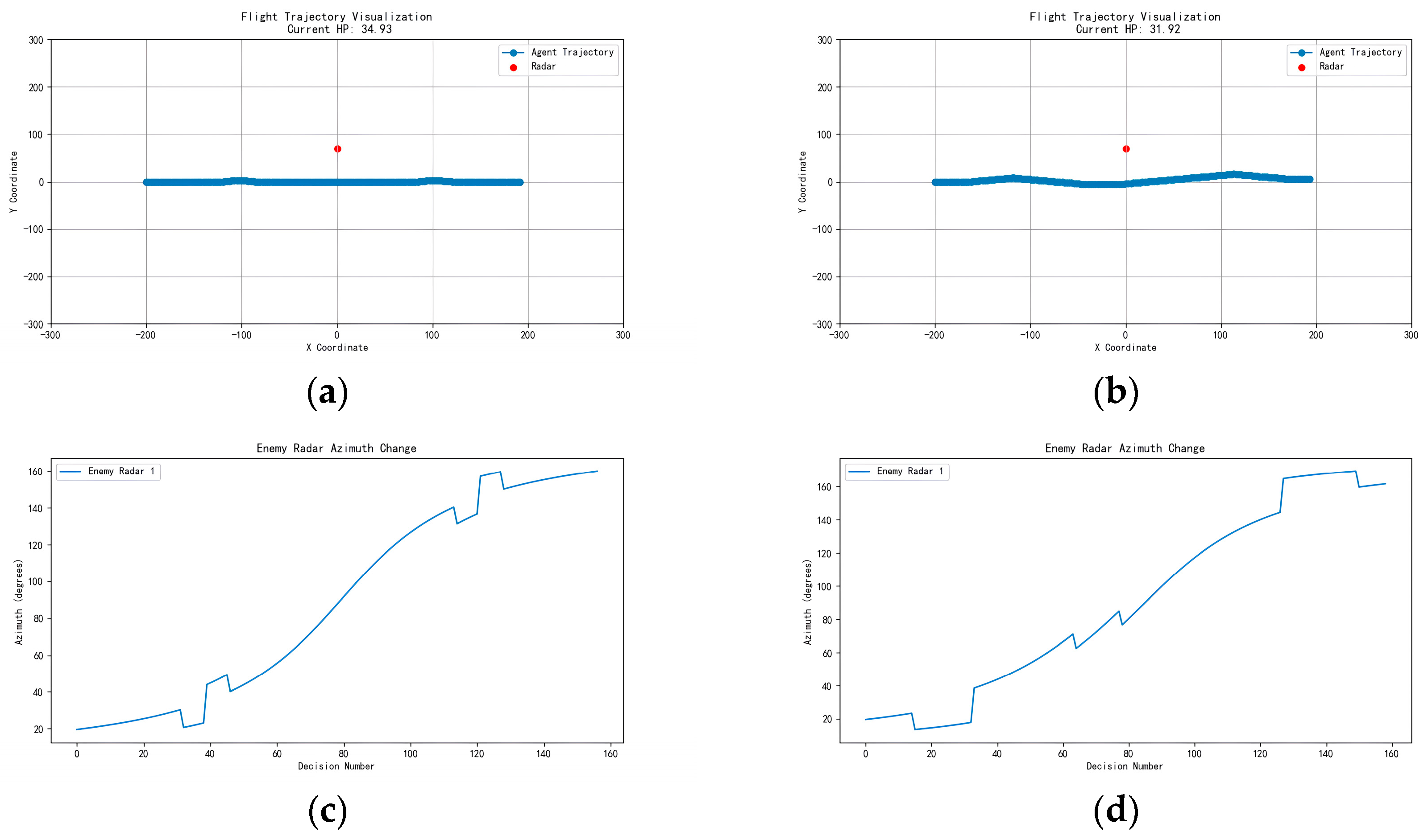
After incorporating the imitation learning, the penetration trajectories before and after free exploration are shown in Figure 40a,b, and the radar’s relative azimuth angles are depicted in Figure 40c,d.

After incorporating the imitation learning, the agent begins free exploration. In Figure 40a,c, it can be observed that the agent very strictly executes the pre-defined turning maneuver strategy, demonstrating good policy fitting during the imitation-learning phase. In Figure 40b,d, despite the trajectory during the free exploration phase involving multiple turns, the agent is still able to make the correct turning decisions at critical moments, indicating that it has grasped the core timing and method of the turning maneuver.

Furthermore, by observing the trajectory, it takes a reasonable trajectory to avoid radar detection, which further verifies the feasibility of the strategy combining imitation learning with free exploration. This strategy not only allows the agent to optimize its decision-making process through self-exploration while imitating expert behavior, but also enhances the efficiency and quality of the task.

6. Conclusions

This study explores innovative approaches in stealth aircraft penetration strategies by integrating advanced computational methods and leveraging prior knowledge for enhanced radar evasion effectiveness. Based on the research conducted in this paper, the following conclusions are drawn:

(1)

The turning maneuver penetration method remains applicable when extending from two dimensions to three dimensions, but it is necessary to minimize the turning angle and speed in planning; this reduction aims to decrease the duration the aircraft exposes its RCS peaks to radar stations at high elevation angles;

(2)

Through extensive analysis of typical threat scenarios, the effectiveness and applicable contexts of turning maneuvers in three-dimensional situations have been determined, which can aid in rapid decision-making; additionally, based on the analysis, a penetration maneuver strategy called the “RVR-TM method” was developed using a decision tree approach;

(3)

Comparative studies of single-radar and triple-radar scenarios under straight trajectory, RVR-TM planned trajectory, and 3D-SALSRM planned trajectory indicate that both methods significantly reduce the radar detection probability compared to straight trajectories, thereby enhancing aircraft survivability; notably, RVR-TM achieves feasible trajectories in far less time than 3D-SALSRM;

(4)

Using reinforcement learning and a 3D trajectory algorithm, this study suggests replacing the Monte Carlo environment with probabilistic deterministic expression and designing state space from prior knowledge; a stealth aircraft decision model using the Proximal Policy Optimization (PPO) algorithm, supplemented by the RVR-TM training method, facilitated rapid 3D decision making, proving effective in achieving radar evasion through prior knowledge.

References

1. Moore, F.W. Radar cross-section reduction via route planning and intelligent control. IEEE Trans. Control Syst. Technol. 2002, 10, 696–700. [Google Scholar] [CrossRef]
2. Liu, H.; Chen, J.; Shen, L.; Chen, S. Low observability trajectory planning for stealth aircraft to evade radar tracking. Proc. Inst. Mech. Eng. Part G J. Aerosp. Eng. 2014, 228, 398–410. [Google Scholar] [CrossRef]
3. Hao, Z.; Zhang, J.; Zhu, F. Three-Dimensional Trajectory Planning for Unmanned Aerial Vehicles in Radar Threat Environments. Flight Dyn. 2010, 28, 47–52. [Google Scholar]
4. Zhang, Z.; Wu, J.; Dai, J.; He, C. A Novel Real-Time Penetration Path Planning Algorithm for Stealth UAV in 3D Complex Dynamic Environment. IEEE Access 2020, 8, 122757–122771. [Google Scholar] [CrossRef]
5. Mi, Y.; Zhang, X.; Sun, J.; Wang, N.; Sun, Y. Research on Combat Aircraft Penetration Trajectory Planning Based on the A* Algorithm; Chinese Society of Aeronautics and Astronautics Stealth and Anti-Stealth Technology Subcommittee: Xi’an, China, 2023. [Google Scholar]
6. Guan, J.; Huang, J.; Song, L.; Lu, X. Stealth Aircraft Penetration Trajectory Planning in 3D Complex Dynamic Environment Based on Sparse A* Algorithm. Aerospace 2024, 11, 87. [Google Scholar] [CrossRef]
7. Lu, X.; Huang, J.; Wu, Y.; Song, L. Influence of stealth aircraft Dynamic RCS peak on radar detection probability. Chin. J. Aeronaut. 2023, 36, 137–145. [Google Scholar] [CrossRef]
8. Zhang, F.; Li, N.; Yuan, R. Robot Path Planning Algorithm Based on Reinforcement Learning. J. Huazhong Univ. Sci. Technol. Sci. Ed. 2018, 46, 65–70. [Google Scholar]
9. Hu, Z.; Wang, Z.; Yang, Y. Optimized PPO Algorithm Based AUV Path Planning. Electron. Opt. Control 2023, 30, 87–102. [Google Scholar]
10. Jiménez, G.A.; Hueso, A.d.l.E.; Gómez-Silva, M.J. Reinforcement Learning Algorithms for Autonomous Mission Accomplishment by Unmanned Aerial Vehicles: A Comparative View with DQN, SARSA and A2C. Sensors 2023, 23, 9013. [Google Scholar] [CrossRef]
11. Zhang, Y.; Wang, H.; Wang, S. Taxiway Path Planning for Aircraft Based on Improved SARSA Algorithm. J. Zhengzhou Univ. Aeronaut. 2024, 42, 43–48. [Google Scholar]
12. Alzorgan, H.; Razi, A.; Moshayedi, A.J. Invited Paper: Actuator Trajectory Planning for UAVs with Overhead Manipulator using Reinforcement Learning. In Proceedings of the 2023 IEEE 34th Annual International Symposium on Personal, Indoor and Mobile Radio Communications (PIMRC), Toronto, ON, Canada, 5–8 September 2023. [Google Scholar]
13. Wang, X.; Zhong, W.; Wang, J. UAV Path Planning and Radio Mapping Based on Deep Reinforcement Learning. J. Appl. Sci. 2024, 2, 201–210. [Google Scholar]
14. Zhang, S.; Dai, Q. Unmanned Aerial Vehicle Path Planning Based on Improved Deep Deterministic Policy Gradients. J. Syst. Simul. 2024, 4, 1–8. [Google Scholar]
15. Bie, T.; Zhu, X.; Fu, Y. Safety priority path planning method based on Safe-PPO algorithm. J. Beijing Univ. Aeronaut. Astronaut. 2023, 49, 2108–2118. [Google Scholar]
16. Peng, Y.; Zhu, Z.; Wei, X. A Channel-Hopping Rendezvous Algorithm based on Reinforcement Q-Learning. Commun. Technol. 2021, 54, 1820–1826. [Google Scholar]
17. Li, H. Based on Meta Reinforcement Learning Research on Behavior Decision Making of Self-Driving Vehicle; Vehicle Engineering, Dalian University of Technology: Dalian, China, 2021. [Google Scholar]
18. Yang, Y.; Zhu, Y.; Hu, C. A Multi-UAV Collision Avoidance Decision-Making Method Based on Reinforcement Learning. Electron. Opt. Control 2023, 30, 112–118. [Google Scholar]
19. Shen, Y. Research on Proximal Policy Optimization Algorithms for Reinforcement Learning Problem; Soochow University: Suzhou, China, 2021. [Google Scholar]
20. Alpdemir, M.N. Tactical UAV Path Optimization under Radar Threat using Deep Reinforcement Learning. Neural Comput. Appl. 2022, 34, 5649–5664. [Google Scholar] [CrossRef]
21. Wang, Z.; Huang, J.; Yi, M. A Stealth–Distance Dynamic Weight Deep Q-Network Algorithm for Three-Dimensional Path Planning of Unmanned Aerial Helicopter. Aerospace 2023, 10, 709. [Google Scholar] [CrossRef]
22. Hameed, R.; Maqsood, A.; Hashmi, A.; Saeed, M.; Riaz, R. Reinforcement Learning-based Radar-evasive Path Planning: A Comparative Analysis. Aeronaut. J. 2022, 126, 547–564. [Google Scholar] [CrossRef]
23. Ma, Z.; Gao, J.; Wu, P. An Improved Deep Reinforcement Learning Algorithm for Cruise Missile Penetration Path Planning. Appl. Electron. Tech. 2021, 47, 11–14, 19. [Google Scholar]
24. Wang, Y.; Li, K.; Zhuang, X.; Liu, X.; Li, H. A Reinforcement Learning Method Based on an Improved Sampling Mechanism for Unmanned Aerial Vehicle Penetration. Aerospace 2023, 10, 642. [Google Scholar] [CrossRef]
Figure 1. Typical Stealth Aircraft 3D RCS.
Aerospace 11 00402 g001
Figure 2. RCS variations with changes in azimuth angle.
Aerospace 11 00402 g002
Figure 3. RCS variations with changes in elevation angle: (a) 0° azimuth angle, (b) 25° azimuth angle, and (c) 35° azimuth angle.
Aerospace 11 00402 g003
Figure 4. Aerodynamic model: (a) lift coefficient variation curve with angle of attack; (b) drag coefficient variation curve with lift coefficient.
Aerospace 11 00402 g004
Figure 5. Results under D = 20 km: (a) full trajectory view; (b) magnified view of the turning section; (c) azimuth angle through the trajectory; (d) elevation angle through the trajectory; (e) cumulative detection probabilities through the trajectory; and (f) single-detection probabilities through the trajectory.
Aerospace 11 00402 g005aAerospace 11 00402 g005b
Figure 6. Results under D = 50 km: (a) full trajectory view; (b) magnified view of the turning section; (c) azimuth angle through the trajectory; (d) elevation angle through the trajectory; (e) cumulative detection probabilities through the trajectory; and (f) single-detection probabilities through the trajectory.
Aerospace 11 00402 g006
Figure 7. Results under D = 100 km: (a) full trajectory view; (b) magnified view of the turning section; (c) azimuth angle through the trajectory; (d) elevation angle through the trajectory; (e) cumulative detection probabilities through the trajectory; and (f) single-detection probabilities through the trajectory.
Aerospace 11 00402 g007
Figure 8. Results under TA = 5°, D = 20 km: (a) full trajectory view; (b) magnified view of the turning section; (c) azimuth angle through the trajectory; (d) elevation angle through the trajectory; (e) cumulative detection probabilities through the trajectory; and (f) single-detection probabilities through the trajectory.
Aerospace 11 00402 g008
Figure 9. Results under TA = 5°, D = 50 km: (a) full trajectory view; (b) magnified view of the turning section; (c) azimuth angle through the trajectory; (d) elevation angle through the trajectory; (e) cumulative detection probabilities through the trajectory; and (f) single-detection probabilities through the trajectory.
Aerospace 11 00402 g009
Figure 10. Results under TA = 20°, D = 50 km: (a) full trajectory view; (b) magnified view of the turning section; (c) azimuth angle through the trajectory; (d) elevation angle through the trajectory; (e) cumulative detection probabilities through the trajectory; and (f) single-detection probabilities through the trajectory.
Aerospace 11 00402 g010
Figure 11. Results under different Mach numbers: (a) full trajectory view; (b) magnified view of the turning section; (c) azimuth angle through the trajectory; (d) elevation angle through the trajectory; (e) cumulative detection probabilities through the trajectory; and (f) single-detection probabilities through the trajectory.
Aerospace 11 00402 g011aAerospace 11 00402 g011b
Figure 12. Results under different radar power factors: (a) full trajectory view; (b) magnified view of the turning section; (c) azimuth angle through the trajectory; (d) elevation angle through the trajectory; (e) cumulative detection probabilities through the trajectory; and (f) single-detection probabilities through the trajectory.
Aerospace 11 00402 g012aAerospace 11 00402 g012b
Figure 13. Results of a cross-side radar scenario: (a) full trajectory view; (b) magnified view of the turning section; (c) azimuth angle through the trajectory; (d) elevation angle through the trajectory; (e) cumulative detection probabilities through the trajectory; and (f) single-detection probabilities through the trajectory.
Aerospace 11 00402 g013
Figure 14. Results of a closely positioned radar scenario: (a) full trajectory view; (b) magnified view of the turning section; (c) azimuth angle through the trajectory; (d) elevation angle through the trajectory; (e) cumulative detection probabilities through the trajectory; and (f) single-detection probabilities through the trajectory.
Aerospace 11 00402 g014
Figure 15. Results of radars positioned further apart: (a) full trajectory view; (b) magnified view of the turning section; (c) azimuth angle through the trajectory; (d) elevation angle through the trajectory; (e) cumulative detection probabilities through the trajectory; and (f) single-detection probabilities through the trajectory.
Aerospace 11 00402 g015
Figure 16. Turning maneuver trajectory after planning.
Aerospace 11 00402 g016
Figure 17. Detection probability of the trajectory after planning under low-power radar.
Aerospace 11 00402 g017
Figure 18. The azimuth and elevation angles to the radar of the trajectory before planning: (a) azimuth angle and (b) elevation angle.
Aerospace 11 00402 g018
Figure 19. Straight trajectory before planning in single-radar scenario.
Aerospace 11 00402 g019
Figure 20. Detection probability of the trajectory before planning under low-power radar.
Aerospace 11 00402 g020
Figure 21. The azimuth and elevation angles to the radar of the trajectory before planning in single-radar scenario: (a) azimuth angle and (b) elevation angle.
Aerospace 11 00402 g021
Figure 22. Turning maneuver trajectory after RVR-TM method planning in single-radar scenario.
Aerospace 11 00402 g022
Figure 23. Detection probability of the trajectory after RVR-TM method planning under a single radar.
Aerospace 11 00402 g023
Figure 24. The azimuth and elevation angles to the radar of the trajectory after RVR-TM method planning in single-radar scenario: (a) azimuth angle and (b) elevation angle.
Aerospace 11 00402 g024
Figure 25. Turning maneuver trajectory after 3D-SASLRM method planning in single-radar scenario.
Aerospace 11 00402 g025
Figure 26. Detection probability of the trajectory after 3D-SASLRM method planning in single-radar scenario.
Aerospace 11 00402 g026
Figure 27. Straight trajectory before planning in a three-radar scenario.
Aerospace 11 00402 g027
Figure 28. Detection probability of the trajectory before planning under a single radar.
Aerospace 11 00402 g028
Figure 29. The azimuth and elevation angles to the radar of the trajectory before planning in a three-radar scenario: (a) azimuth angle and (b) elevation angle.
Aerospace 11 00402 g029
Figure 30. Turning maneuver trajectory after RVR-TM method planning in a three-radar scenario.
Aerospace 11 00402 g030
Figure 31. Detection probability of the trajectory after RVR-TM method planning under three radars.
Aerospace 11 00402 g031
Figure 32. The azimuth and elevation angles to the radar of the trajectory after RVR-TM method planning in a three-radar scenario: (a) azimuth angle and (b) elevation angle.
Aerospace 11 00402 g032
Figure 33. Turning maneuver trajectory after 3D-SASLRM method planning in a three-radar scenario.
Aerospace 11 00402 g033
Figure 34. Detection probability of the trajectory after 3D-SASLRM method planning in a three-radar scenario.
Aerospace 11 00402 g034
Figure 35. Decision model based on PPO algorithm.
Aerospace 11 00402 g035
Figure 36. Results under different distance penalties: (a) with no distance penalty and (b) with distance penalty.
Aerospace 11 00402 g036
Figure 37. Azimuth under different action penalties: (a) with no action penalty and (b) with action penalty.
Aerospace 11 00402 g037
Figure 38. Trajectory and azimuth with reward shaping: (a) trajectory and (b) azimuth angle.
Aerospace 11 00402 g038
Figure 39. Process of imitation learning.
Aerospace 11 00402 g039
Figure 40. Results after incorporating imitation learning: (a) trajectory before incorporating imitation learning; (b) trajectory after incorporating imitation learning; (c) azimuth angle before incorporating imitation learning; and (d) azimuth angle after incorporating imitation learning.
Aerospace 11 00402 g040