Abstract
Computational simulations of three-dimensional flow around a NACA 0018 wing with an aspect ratio of were carried out by using the Unsteady Reynolds-Averaged Navier–Stokes (URANS) equations with the Shear-Stress Transport turbulence model closure. Simulations were performed to capture aerodynamic stall hysteresis by using the developed pseudo-transient continuation (PTC) method based on a dual-time step approach in CFD OpenFOAM code. The flow was characterized by incompressible Mach number and moderate Reynolds number . The results obtained indicate the presence of noticeable aerodynamic hysteresis in the static dependencies of the force and moment coefficients, as well as the manifestation of bi-stable flow separation patterns, accompanied by the development of asymmetry in the stall zone. The URANS simulation results are in good agreement with the experimental data obtained for the NACA 0018 finite-aspect-ratio wing in the low-speed wind tunnel under the same test conditions. A new phenomenological bifurcation model of aerodynamic stall hysteresis under static and dynamic conditions is formulated and is proven to be able to closely match the experimental data.
1. Introduction
Aerodynamic stall phenomena are important in many engineering applications that influence critical operating limits and system performance. Aerodynamic hysteresis, which is observed both in experiments and in computational simulations under static and dynamic conditions, is an important feature of the stall region [1,2,3]. This phenomenon has been observed in wind tunnel tests for flow around two-dimensional profiles such as NACA 0012 and 0018 for low Reynolds numbers, i.e., , as shown in [4,5,6]. The existence of aerodynamic hysteresis in a thin airfoil with leading edge modifications for moderately high Reynolds numbers, , was shown in [7]. Other studies with three-dimensional wing configurations have also shown the existence of multiple branches of aerodynamic loads in the presence of static hysteresis [8,9]. Some successful simulations of aerodynamic static hysteresis and the challenges involved in such flows at high angles of attack were discussed in [10,11].
Stall prediction using wind tunnel tests or computer simulations is challenging due to the high sensitivity of flow separation to experimental testing conditions or computational models and solvers, respectively. Strong turbulence in the wind tunnel flow and vibrations of the test model mounting system can cause premature transitions between the branches of static hysteresis [6]. In computational simulations, there is also observed sensitivity to the numerical solver, grid resolution, turbulence model, etc. [11]. Despite the complications, it is important to improve the understanding of the flow physics of the static hysteresis phenomenon to develop a more reliable modelling of stall aerodynamics. Applications where static hysteresis exists range from wind turbines and micro air vehicles operating at low Reynolds numbers to the problem of in-flight loss of control (LOC-I) of transport aircraft, for which the modelling of stall/post-stall aerodynamics at high Reynolds numbers is required [12].
There are many wind tunnel results that show static hysteresis in the separated flow region. For instance, the occurrence of static aerodynamic hysteresis in flow around a NACA 0018 airfoil in the range of Reynolds numbers from to was shown in [4,5,13]. It was also shown that aerodynamic static hysteresis can exists even at high Reynolds numbers, , and may be even enlarged with a circular bump on the leading edge of the pressure side of the airfoil [7]. CFD predictions of such static hysteresis phenomena in 2D airfoils using the URANS equations in OpenFOAM [14,15] with the SA (1-eqn) and SST (2-eqns) turbulence models have also been successful [13,16]. The use of an algebraic turbulence model such as the Baldwin–Lomax model was also deemed sufficient for capturing the static hysteresis of a NACA 0012 airfoil at but was associated with a very strong buffeting, even after introducing a special stabilizing numerical procedure [10].
In this paper, we consider three-dimensional separated flow with the existence of aerodynamic static hysteresis for a NACA 0018 finite-aspect-ratio wing with at moderate Reynolds numbers, i.e., and . For the conducted URANS simulations with the use of the SST turbulence model, open-source CFD OpenFOAM code was used. The obtained simulation results were compared with wind tunnel data from [8]. To the best knowledge of the authors, these are the first simulation results of aerodynamic static hysteresis loops for a three-dimensional wing configuration matching the experimental data and showing the development of flow asymmetry at high angles of attack. This shows the applicability of URANS simulations for the evaluation of separated flows forming with bi-stable flow structures and static hysteresis in aerodynamic loads. The simulations were carried out by using a pseudo-transient continuation algorithm-based dual-time solver developed in OpenFOAM, as proposed in [17]. The methodology involves driving the residuals of segregated equations to zero (or at least to a truncation error) in every time step to ensure full convergence of the flow variables [14,15].
This paper also introduces a novel phenomenological method for modelling static hysteresis manifesting bi-stable separated flow structures. A concept of such bifurcation modelling of static hysteresis was proposed in [18], and some of its implementations were previously discussed in [13,19,20,21].
The application of the proposed phenomenological model in this paper and its validation against experimental results are presented in Section 4. The CFD simulation results are presented in the paper as follows: The computational framework, including the geometry, grid and other numerical setup details, is discussed in Section 2. The computational results for static hysteresis obtained for Reynolds numbers of and by using OpenFOAM are shown in Section 3. This section also includes the skin friction visualization patterns and three dimensional streamlines for bi-stable flow structures. The concluding remarks and future work are presented in Section 5.
2. Computational Framework
In this section, the discussion revolves around the computational framework employed for simulating static and dynamic hysteresis. This includes the geometrical attributes of the NACA 0018 wing, the governing equations, and the numerical settings applied in OpenFOAM.
A NACA 0018 finite-aspect-ratio wing with was made up from the two-dimensional NACA 0018 section profile with rounded tips at its ends. The wing span of the NACA 0018 was measured as m, and the chord length was m. A blunt trailing edge similar to that in the wind tunnel wing geometry was implemented. The incorporation of rounded tips aimed to facilitate smooth flow attachment to the wing edges and support the proper development of wing tip vortices. The adopted geometry of the considered wing is illustrated in Figure 1. The boundaries of the virtual wind tunnel were positioned at a distance of 50 chord lengths in the upstream, downstream, and sideways directions. Consequently, there was no need for blockage corrections in the Computational Fluid Dynamics (CFD) results obtained with this setup.
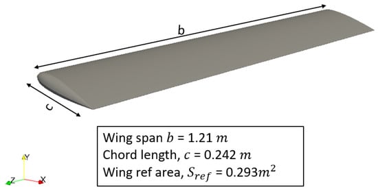
Figure 1.
NACA 0018 wing geometry.
The inlet was subjected to a Dirichlet velocity-inlet boundary condition, complemented by a Neumann-type zero-gradient pressure boundary condition. Meanwhile, at the outlet, a zero-gradient velocity outlet boundary condition was applied, and the pressure was set to a fixed value of = 0. Slip boundary conditions were adopted for the wind tunnel walls. To replicate wind tunnel conditions, the turbulent kinetic energy at the inlet was set to a fixed value based on a turbulence intensity of . For the solid rotating surfaces, specifically the NACA 0018 wing, a “movingWallVelocity” boundary condition was implemented to ensure a zero-flux condition during dynamic or quasi-steady oscillations.
The computational grids were generated by using ICEM CFD software, incorporating an O-grid topology for the seamless wrapping of the O-type blocking around the wing with a blunt trailing edge. This approach facilitates the creation of a high-quality, structured grid with favourable cell determinant values for the hexahedral cells. Utilizing O-type blocking ensures a well-defined boundary layer, maintaining optimal values for cell skewness and orthogonality. The ratios of cell area and volume transitions fell within the range of 0.8–1.2, allowing for a maximum change of 20 percent. This ensured that large gradients in flow scalar and vector variables were avoided during the simulation. The boundary layer comprised 30 adjacent layers with a growth rate of . The height of the first cell layer was determined by a non-dimensional wall distance of , enabling the use of a no-wall-function, low-Reynolds-number approach. Following a thorough grid independence study, a mesh size of 3.5 million elements was found to be sufficient for this study, as shown in Figure 2.
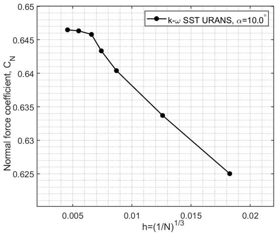
Figure 2.
Normal force coefficient () variation against grid resolution parameter (h) from the conducted mesh independence study.
The flow conditions, characterized by a relatively low Mach number, , allowed for the consideration of incompressible fluid flow. The Navier–Stokes (NS) equations governing incompressible fluid flow are the continuity (Equation (1)) and the momentum (Equation (2)) formulas:
For flow conditions characterized by high Reynolds numbers, the computational demands associated with the Direct Numerical Simulation (DNS) of Equations (1) and (2) typically surpass the current computational capabilities. To address the effects of turbulence in a more computationally feasible manner, the Unsteady Reynolds-Averaged Navier–Stokes (URANS) equations are often employed. These represent a time-averaged approximation of the Navier–Stokes equations, with the averaging process introducing additional terms known as Reynolds stresses. Describing these stresses necessitates the inclusion of empirical equations, either algebraic or differential, to close the computational model. The majority of URANS turbulence models rely on an eddy viscosity concept, analogous to the kinematic viscosity of fluids, to characterize the turbulent mixing or diffusion of flow momentum. In linear turbulence models, the Reynolds stresses resulting from the averaging are modelled by using the Boussinesq assumption (Equation (3)):
In this study, the SST (Shear-Stress Transport) two-equation turbulence model, as proposed by Menter [22], was utilized. This model is widely applied in aeronautical applications, particularly for external aerodynamics involving adverse pressure gradients and strongly separated flow conditions [11,22]. The authors have also previously employed the SST model for capturing static hysteresis phenomena for the NACA 0018 2D airfoil [13]. The SST model solves two equations, one for the turbulent kinetic energy (k) and the second for evaluating , which represents the specific dissipation rate of turbulence.
According to a meticulous evaluation and the testing of various finite volume schemes and solvers available in OpenFOAM, as outlined in Table 1, the Pre-conditioned Conjugate (PCG) solver coupled with the Geometric Algebraic Multi-Grid method (GAMG) as a pre-conditioner seemed as the most efficient algorithm for driving unsteady residuals to zero at each time level. By employing the GAMG pre-conditioner with 10–30 iterations and applying the pre- and post-smoothing of residuals for 2–3 levels, it was observed that only 10–30 iterations of the PCG solver were required to reduce the residual (in the outer iterations) to nearly zero. The gradients of the flow quantities were computed by using the second-order accurate Gauss linear scheme with limiters based on cell centre values. The divergence of the vector velocity field and the scalar turbulent quantities was estimated with second-order accuracy by using the “cellLimited Gauss linear” scheme in OpenFOAM. A linear interpolation scheme was utilized for estimating the contribution of the cell centre variables to the faces.

Table 1.
Finite volume solvers in OpenFOAM used in the study.
The estimation of the time derivatives in OpenFOAM for the case studies involved in this research was accomplished by using the dual-time stepping method, which has been well established for steady-state problems [23,24]. More particularly, the time integration technique proposed in [17], which has been verified and tested for several dynamic hysteresis and quasi-steady hysteresis cases, was adopted.
3. Computational Results
In this section, the results of computational simulations for the flow around a NACA 0018 finite-aspect-ratio wing with are presented and discussed. The first case explores the aerodynamic stall hysteresis obtained during very slow, quasi-steady sinusoidal motion with and large amplitude of motion, –, at two distinct Reynolds numbers, and . Additionally, insights into the development of flow asymmetry for high angles of attack are also provided. In the second case, the influence of the frequency of sinusoidal motion on aerodynamic stall hysteresis is examined. The wing motion for both cases with sinusoidal motion described by with reduced frequency is detailed in Table 2.
Table 2.
Summary of the considered case studies.
3.1. Case 1—Effect of Reynolds Number and Development of Flow Asymmetry
The variation in the normal force coefficient () at with physical time is shown in Figure 3. The angle-of-attack variation during this motion is also mapped on the same figure. Notably, after a nearly linear increase in until s, there was a substantial drop after reaching . This was followed by a more moderate increase in into the higher-angle-of-attack region, i.e., . By comparing the values at the same angle of attack during the increase and decrease in angle-of-attack phases, the development of aerodynamic stall hysteresis and bifurcation of aerodynamic loads are distinctly evident in Figure 3.
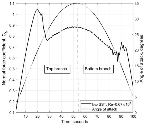
Figure 3.
Variation in normal force coefficient (; primary y-axis) and angle of attack (; secondary y-axis) with physical time for static hysteresis loop obtained at .
The acquired computational results for the two different Reynolds numbers of and are shown in Figure 4. OpenFOAM simulation results for at demonstrate good agreement with the wind tunnel data from [8] until , and between and , the values (solid black line) slightly exceed the wind tunnel values (filled black markers). Note that the deviation in between CFD and wind tunnel data in this range of angle of attack is very small; for instance, at , the difference in the normal force coefficient between the wind tunnel data and CFD results is only . The computational simulation results also show that the fully developed stall conditions leading to an abrupt drop in occur at almost identical angle of attacks, i.e., . It is also evident that the level of the abrupt drop in the normal force coefficient at critical angle of attack is also in agreement with the wind tunnel data from [8]. Some difference between CFD and wind tunnel data occurs in the higher-angles-of-attack region of , where the coefficient is slightly shifted up due to the CFD results having practically the same slope.
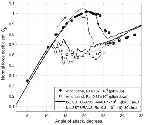
Figure 4.
Normal force coefficient () vs. () during the pitch-up and pitch-down phases: CFD simulations and wind tunnel data from [8].
During the pitch-down motion, the CFD results demonstrate significantly lower values for the same angle of attack (), which is identical to the wind tunnel data. The maximum difference in between the top and bottom branches occurs at , where and , leading to a noticeable drop in the normal force coefficient: . The static hysteresis loop obtained at this Reynolds number () (see solid black line) is almost as wide as the static hysteresis obtained in the wind tunnel (see circle markers). The extent of similarity in the normal force coefficient variation between the CFD and wind tunnel data during the pitch-up and pitch-down phases gives the certainty that CFD URANS simulations could be used to capture such nonlinear bifurcation phenomena with a reasonable level of accuracy.
The nature of the phenomenon of static aerodynamic hysteresis lies in the possibility of the emergence of bi-stable separated flow structures over the NACA 0018 wing in a certain range of angle of attack in the stall zone. The flow in both cases is separated but has different flow patterns, clearly described by the skin friction contours from simulations and experiment shown in Figures 6 and 8, respectively. The flow separation on the lower branch of the static hysteresis is more developed towards the leading edge of the wing, which leads to a more significant loss of the normal force coefficient due to the loss of the suction pressure peak.
OpenFOAM simulations were also conducted at a lower Reynolds number, . The grid used for simulations at was manipulated in the boundary layer region to adjust Y+ consistently for the lower-Reynolds-number flow conditions. The obtained CFD results for , shown in Figure 4 (dotted black line), demonstrate an early-onset of fully developed stall conditions with an abrupt drop in the normal force coefficient 2 degrees earlier than that for the case with . An approximately -degree-wide hysteresis loop was obtained at Reynolds number . Note that there are plenty of 2D experimental and CFD results for NACA 0018 airfoil hysteresis at [4,5,13], but not for the 3D NACA 0018 wing. The slightly decreased maximum normal force coefficient () and earlier stall at the lower Reynolds number of indicates that the computational results acquired are aligned with the physical intuition.
The pitching moment coefficients () obtained from the CFD URANS simulations by using OpenFOAM for two different flow Reynolds numbers are illustrated in Figure 5. Similar to the normal force coefficient (), the obtained CFD results demonstrated noticeable static hysteresis in the pitching moment coefficient () in both cases, i.e., and .
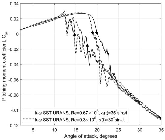
Figure 5.
Pitching moment coefficient () vs. during the pitch-up and pitch-down phases.
The CFD simulations demonstrate the presence of static stall hysteresis in the aerodynamic coefficients and in the range of angle of attack . To gain a physical insight into the origin of the static hysteresis phenomenon, flow visualization is extremely important. Figure 6 shows the variation in the skin friction coefficient () contours and the surface streamlines for the NACA 0018 3D finite-aspect-ratio wing. For easier demonstration, the visualizations were conducted at specific waypoints in the variation in against during the pitch-up and pitch-down phases, denoted by A–E, as shown in Figure 6. Point A in Figure 6 shows the attached flow conditions at with minor trailing edge separation, as one would expect on this finite-aspect-ratio wing at the beginning of flow separation. With the increase in angle of attack to (see point B in Figure 6) on the top branch, the surface streamlines seem to reverse from the trailing edge curving towards the central portion of the wing surface; simultaneously, the flow from the leading edge is still attached and travelling towards the trailing edge of the wing. The reversed flow from the trailing edge and the attached flow from the leading edge meet in a central location on the wing, forming a confluence flow towards the middle of the wing, where they end in two focuses forming the basis for a 3D arch-type vortex.
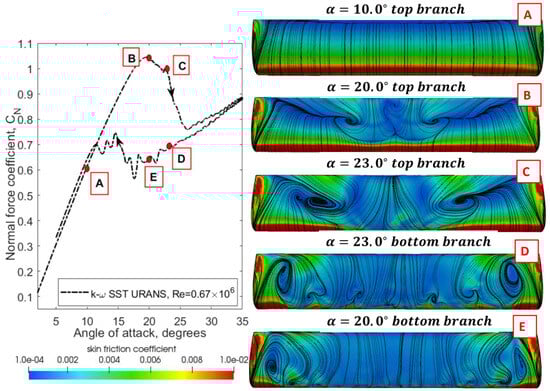
Figure 6.
The contours of the skin friction () superimposed on surface streamline patterns on the NACA 0018 wing during the pitch-up and pitch-down phases of aerodynamic static hysteresis.
As the angle of attack is further increased to (see point C in Figure 6) on the top branch, the arch vortex core strengthens, becomes wider and also deviates towards the opposite ends of the wing in the direction of the wing tips. At this angle of attack, the flow is only attached close to the wing tips on the leading edge and is fully detached from the central part of the leading edge. In the pitch-down phase, for the same angle of attack of (see point D in Figure 6) on the bottom branch, the flow is almost fully detached from the leading edge and the main arch vortex widens and moves close to the wing tips.
The surface streamlines also show a few additional small arch vortices on top of the wing close to the leading edge. The flow is practically fully separated from the wing at points D and E on the bottom branch of static hysteresis (see Figure 6). Three-dimensional flow topology including the presence of arch-type vortices at few selected angle of attacks on the top and bottom branches of static hysteresis is demonstrated in Figure 7.
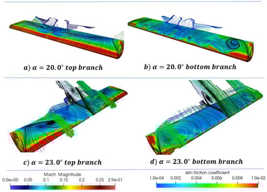
Figure 7.
Three-dimensional streamlines of velocity field and contours of skin friction () superimposed on surface streamline patterns on NACA 0018 wing during pitch-up and pitch-down phases at and .
Flow visualization in wind tunnel using the oil flow images during static hysteresis from [25] shows qualitative agreement with computationally predicted flow patterns. This comparison, shown in Figure 8, gives some level of confidence in using URANS simulations for predicting such complex and nonlinear bifurcation phenomena.
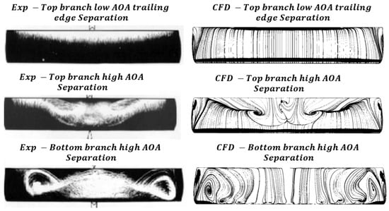
Figure 8.
Qualitative comparison of wind tunnel oil flow visualization [25] and CFD surface streamline patterns on the top and bottom branches of aerodynamic hysteresis.
An important feature of high-angle-of-attack aerodynamics observed in experiments is the development of aerodynamic asymmetry [8]. The onset of aerodynamic asymmetry occurred in the conducted CFD simulations even with a perfectly symmetric grid. For the simulation carried out at , the onset and development of aerodynamic asymmetry was correlated with the presence of arch vortices on the top branch of static hysteresis and during reattachment flow transition from the bottom branch of static hysteresis. In order to estimate the maximum asymmetry from the CFD simulations, the rolling moment coefficient () and the yawing moment coefficient () were extracted from the CFD simulations and are shown in Figure 9.
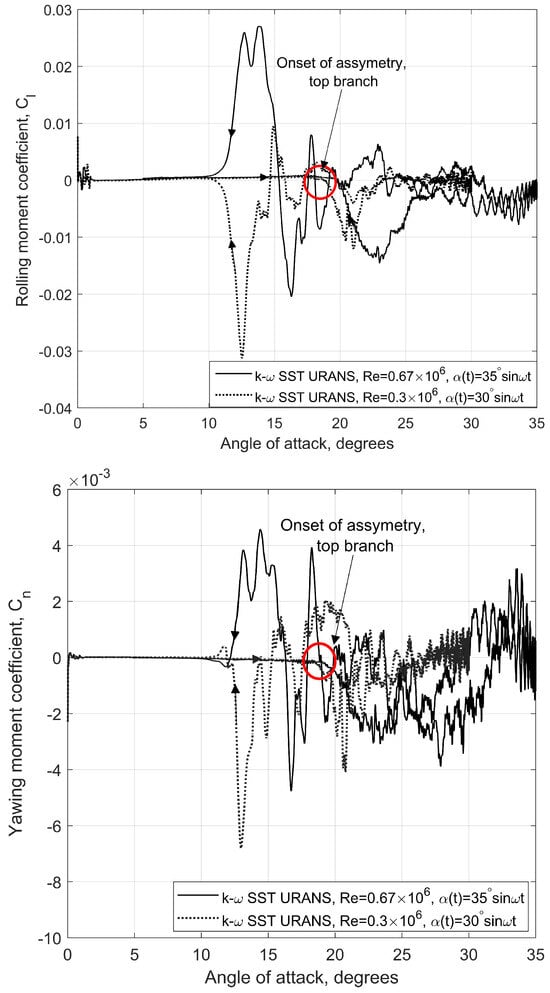
Figure 9.
Rolling and yawing moment coefficients ( and ) from CFD simulations vs. during the pitch-up and pitch-down phases.
During the pitch-up phase, the onset of aerodynamic asymmetry occurred at approximately . The maximum asymmetry in both and during the pitch-up phase took place at , which correlates with the maximum normal force coefficient (). The peaks of asymmetry developed during the pitch-down phase, and this phenomenon was highly evident in the range of .
Flow visualizations corresponding to the onset of aerodynamic asymmetry are shown on the right side of Figure 10, and the variation in the rolling moment coefficient () vs. angle of attack is shown on the left side of the same figure. Point A and point C correspond to the same angle-of-attack points shown in Figure 6, i.e., and . Points F and G are new, and they correspond to the pitch-down phase at positive and negative peaks of aerodynamic asymmetry. The flow visualizations clearly show the process of reattachment of the flow and a highly variable instantaneous profile of skin friction contours.
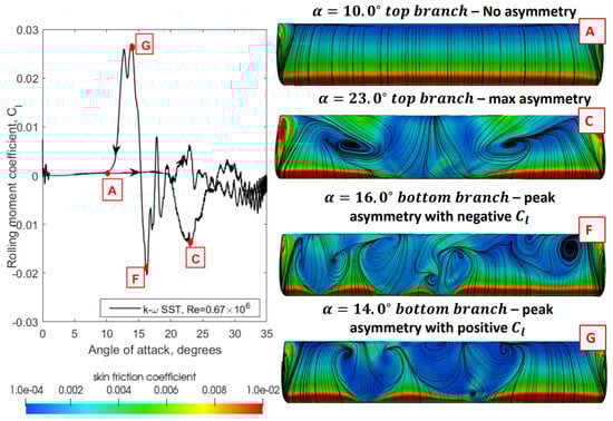
Figure 10.
Contours of skin friction () superimposed on surface streamline patterns on NACA 0018 wing during pitch-up and pitch-down phases of aerodynamic static hysteresis showing development of flow asymmetry.
3.2. Case 2—Influence of Rate of Change in Angle of Attack on Aerodynamic Hysteresis
The effect of different rates of change in the angle of attack () on the normal force coefficient () around the static hysteresis region is presented in Figure 11. For this analysis, the angle of attack was changed periodically with the mean angle of attack of , amplitude of and three different frequencies (, and , where rad/s). The maximum rates of angle-of-attack change for the results presented in Figure 11 are deg/s (dotted line), deg/s (dashed line) and deg/s (solid line), respectively.
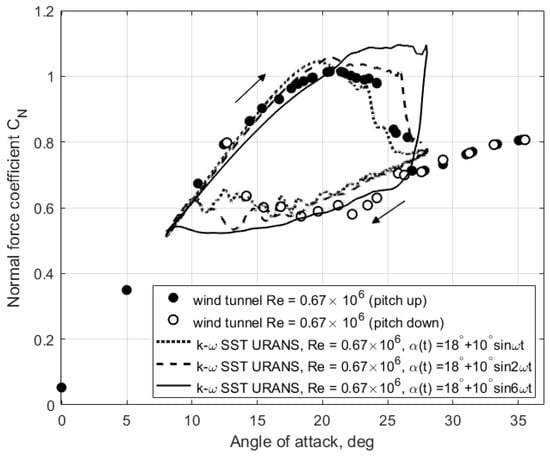
Figure 11.
Normal force coefficient () from computational simulations at different rotational frequencies with and amplitude .
The obtained computational results demonstrate that the simulations conducted at = deg/s and 1.0 deg/s are suitable for capturing the top branch of static hysteresis, whilst the simulation conducted at = 3.0 deg/s slightly overpredicts the maximum value of the normal force coefficient. Note that the quasi-static simulations are extremely computationally expensive at very low , as a transient method must be used, which requires the dual-time solver to iterate many cycles to reduce residuals to zero. For the bottom branch, both = deg/s and 1.0 deg/s demonstrate identical results and are in good agreement with the experimental data. Figure 11 shows that the impact of the rate of angle-of-attack change () is also significant. More information about the dynamic hysteresis effects in aerodynamic loads due to can be found in [1,2].
4. Phenomenological Bifurcation Model
This section presents a phenomenological model of aerodynamic hysteresis, reflecting the empirical properties of aerodynamic loads in the stall zone. The proposed formulation for the phenomenological model is adapted to the available experimental data [8] and the CFD simulation results presented above.
The formulation of the phenomenological model should reflect the effects observed in experiments and computer simulations of the delay in the onset of flow separation, as well as its reattachment, compared with static conditions. It was shown that the flow separation delay is proportional to the rate of change in the angle of attack () due to the improvement in the pressure gradient in the region of the leading edge [1]. Flow reattachment when returning to lower angles of attack also exhibits similar behaviour. A key feature of the phenomenological model is the need to reflect the existence of bi-stable separated structures that create static hysteresis loops and also dynamic transitions between branches of static hysteresis under unsteady conditions.
The phenomenological model, originally proposed in [18], was based on the use of a first-order nonlinear dynamic system, including a folded equilibrium surface with bifurcation points bounding the static hysteresis zone, representing flows with a non-unique structure. A simplified model [18] for aerodynamic loads taking into account a single separated flow structure in the stall zone, presented in [26], demonstrated good agreement with experimental data obtained in a wind tunnel for a number of delta wings, as well as for aircraft performing Cobra manoeuvrers. The used representation is based on the introduction of an internal variable (x) characterising the position of the vortex breakdown or flow separation point governed by a first-order linear differential equation characterising variation in the internal state variable under transitional motion conditions. The delay of stall was described by using the delay argument . Recently, this delay–relaxation model has attracted the attention of researchers and showed its efficiency in many applications, ranging from separation flow control and gust alleviation [5,27] to transport aircraft dynamic manoeuvrers [28].
With introduction of the normalised internal state variable (), the aerodynamic loads depend not only on the angle of attack () and its rate of change () but also on the state variable (x); for example, the normal force coefficient in the stall region can be represented with the nonlinear function , reflecting the influence of the internal variable (x) on the aerodynamic loads. This general function should have the following properties: and , where is the dependence of the normal force coefficient under attached flow conditions, which is extended above the stall region, and represents the dependence of the normal force coefficient under fully separated flow conditions, which is extended below the stall region (see Figure 12).
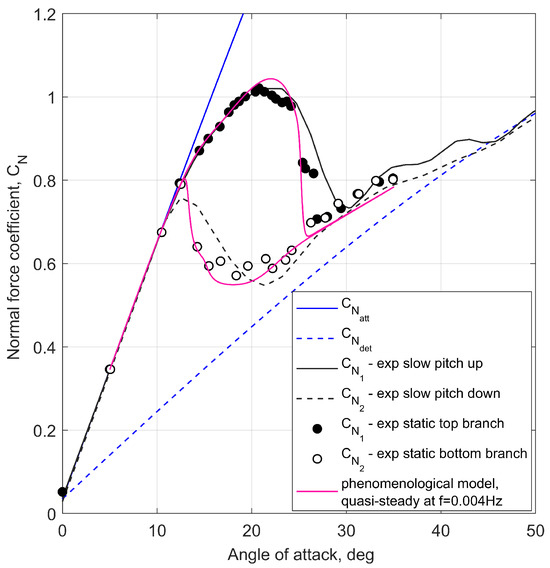
Figure 12.
Normal force coefficient () of NACA 0018 wing at : (1) static test points, (2) slow pitch-up and pitch-down measurements, (3) approximation lines for fully attached and fully detached flow conditions ( and ) and (4) phenomenological model predictions under quasi-steady conditions.
In case of a single flow structure, the dynamic behaviour of the internal state variable () is described by the following first-order linear relaxation differential equation:
where is a normalised internal state variable characterising the location of flow separation; corresponds to the conditions of an attached flow and to the conditions of a completely detached flow; characterises the location of flow separation under static conditions; is the delayed angle of attack, where the delay is proportional to the rate of change in the angle of attack ; and and are the time constants, which characterise the relaxation process and the delay effect, respectively.
The transition of flow from attached conditions to completely detached conditions in the dependence considers that most of the normal force is generated in the area close to the leading edge of the wing; the following approximation is accepted:
where . According to the Kirchhoff formula for a fully separated flow with a constant pressure zone behind an airfoil [5,26,28], this function, by considering Equation (5), is represented as . This formula shows that about of the normal force coefficient () is generated in the immediate vicinity of the leading edge, . This amount of is lost upon transition to a completely separated flow regime, which is characteristic of the lower branch of static hysteresis.
There is a wealth of experimental data showing the existence of static aerodynamic hysteresis in the stall zone, similar to the experimental and simulation results for the NACA 0018 presented in this paper. To model static aerodynamic hysteresis formula (Equation (4)) should become nonlinear as
and the steady states in this system must be represented by a folded curve with two turning points bounding the static aerodynamic hysteresis loop. For this, the nonlinear function in Equation (6) can be represented as a third-order polynomial with respect to the internal variable (x) in following form , as it was used in [20]. Note that Equation (6) is converted into Equation (4) when , and . By using experimental data for static conditions and oscillations at different amplitudes and frequencies, the model coefficients and in Equation (6) can be formally identified by minimizing a positive definite cost function consisting of the differences between the results of the phenomenological model and the experimental data. The details of such identification can be found in [20].
In this work, we present a geometric approach to the formation of a folded curve of equilibrium solutions to Equation (6) for modelling static aerodynamic hysteresis, which is visually implemented below by trial and error, proving the possibility of developing a formal identification procedure of the model parameters for any particular stall condition.
We modify Equation (4) to the following nonlinear form:
where is the hysteresis morphing function and is the saddle disturbance function. The choice of these two functions, which we present below, is based on the creation of three different equilibrium solutions in the stall region by shaping the function as a closed curve in the form of an ellipse and the function , which is non-zero only in the vicinity of two saddle points of a nullcline set of points defined by the equation ; the function specifies the relaxation time in various stationary states of the phenomenological model.
Figure 13 graphically presents major constructions in designing the nonlinear functions in Equation (7). The dashed lines represent the nullcline set of points defined by the equation . The function is crossing the ellipse defined by the morphing function in two saddle points, and . These two saddle points are structurally unstable, and the function applied in the vicinity of the saddle points transforms the nullcline set of points into a continuous folded curve, which shapes a skeletal function for static hysteresis. This curve includes two stable branches of static hysteresis, one on the top, with , and one on the bottom, with . The intermediate branch (red segment) represents an unstable solution to Equation (7), which separates regions of attraction of stable branches (two black segments). Two fold bifurcation points, and , on the skeletal curve indicate jump-like transition from one stable branch of static hysteresis to another stable branch depending on the direction of the angle-of-attack variation. The presented skeletal hysteresis function was adapted to the experimental positions of for the top and bottom branches of static hysteresis: and . More details about the constructed functions are given in Appendix A.
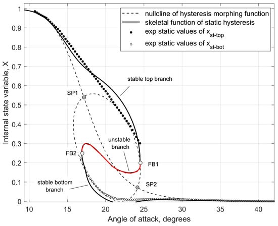
Figure 13.
Phenomenological model skeletal function of static hysteresis based on experimental data.
The characteristic time scale () in the case of Equation (7) is now expressed as
where . This means that when approaching bifurcation points of static hysteresis and , the relaxation time approaches infinity (). This explains the significant expansion of the hysteresis loops under unsteady conditions with very slow variation in the angle of attack ( deg/s) (see Figure 11).
Figure 12 shows that the constructed nonlinear functions shown in Figure 13 accurately model the quasi-static hysteresis, showing good matching with the experimental data. Three different cases of dynamic hysteresis were modelled: (a) the loop around the static hysteresis zone (shown in Figure 14), (b) the loop on the top branch of reaching bifurcation point (shown in Figure 15) and (c) the loop on the bottom branch of reaching bifurcation point (shown in Figure 16). The images on the left in Figure 14, Figure 15 and Figure 16 show dynamic variations in the internal state variable () with respect to the skeletal function of static hysteresis. The phenomenological modelling results in all three cases (a–c) are very close to the experimental wind tunnel data for different amplitudes and frequencies of oscillation. The tuning of the nonlinear function in the model equation (Equation (7)) was carried out manually by a trial-and-error method for an ensemble of the considered processes. A formal mathematical approach for the parameter identification of phenomenological bifurcation models needs further research.
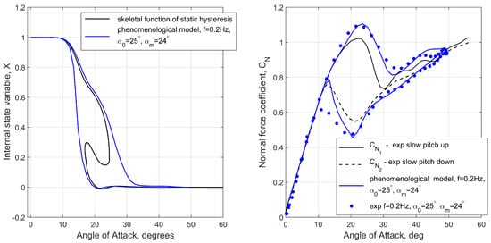
Figure 14.
Internal state variable () and normal force coefficient (): comparison of phenomenological results with experimental data at , where Hz.
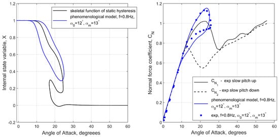
Figure 15.
Internal state variable () and normal force coefficient (): comparison of phenomenological results with experimental data at , where Hz.
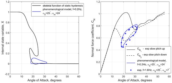
Figure 16.
Internal state variable () and normal force coefficient (): comparison of phenomenological results with experimental data at , where Hz.
5. Conclusions
The use of the Unsteady Reynolds-Averaged Navier–Stokes equations with the Shear-Stress Transport turbulence model allowed us to adequately simulate the aerodynamic characteristics of a NACA 0018 wing with an aspect ratio of in the stall zone with manifestation of bi-stable separation flow structures and static hysteresis. The flow was characterized by incompressible Mach number and Reynolds numbers and . The obtained simulation results indicate the presence of noticeable aerodynamic hysteresis in the static dependencies of the normal force and pitching moment coefficients, which are in good agreement with the wind tunnel data. Qualitative agreement between the CFD-obtained surface streamlines on the NACA 0018 wing and the wind tunnel surface oil flow visualization was shown for the top and bottom branches at various angles of attack. The onset of the aerodynamic asymmetry of separated flow and associated non-zero rolling and yawing moments are also qualitatively similar in CFD simulations and in the experiment. The proposed phenomenological model of aerodynamic stall hysteresis under static and dynamic conditions makes it possible to achieve aerodynamic responses very close to the results of wind tunnel tests. The formal procedure for identifying the parameters of the proposed phenomenological bifurcation model requires special effort.
Author Contributions
Conceptualization, M.S. and M.G.; Methodology, M.S. and M.G.; Software, N.A.; Validation, N.A. and M.G.; Investigation, N.A. and M.G.; Writing—original draft, M.S.; Writing—review & editing, M.S. All authors have read and agreed to the published version of the manuscript.
Funding
This research received no external funding.
Data Availability Statement
The data presented in this study are available on request from the corresponding author.
Conflicts of Interest
The authors declare no conflicts of interest.
Appendix A
This appendix provides further details on the phenomenological modelling presented in Section 4.
Function in Equation (7) is formulated as
where is the inflection point of the curve.
The hysteresis morphing function () is represented as
where and are the vertical centre position and the vertical semi-diameter of the ellipse, and and are the horizontal centre position and the horizontal semi-diameter of the ellipse. The ellipse can be shifted from the inflection point vertically and horizontally; for example, in Equation (A2) shifts the ellipse horizontally.
To better fit the experimental data, a change in the orientation of the ellipse may be required. In the implemented model, the hysteresis morphing function was modified as follows:
where is approximately a rotation angle of the ellipse (see Figure 13).
The saddle disturbance function () is shaped as a spline bell-like function and applied at two saddle points, and :
where is the maximum magnitude of and is
where and define the location of a saddle point (shown in Figure 13).
References
- Ericsson, L.E.; Reding, J.P. Unsteady Airfoil Stall; Technical Report CR-66787; NASA: Washington, DC, USA, 1969.
- Ekaterinaris, J.A.; Platzer, M.F. Computational Prediction of Airfoil Dynamic Stall. Prog. Aerosp. Sci. 1997, 33, 759–846. [Google Scholar] [CrossRef]
- Hoak, D.E. The USAF Stability and Control DATCOM; Technical Report TR-83-3048; Air Force Wright Aeronautical Laboratories: Dayton, OH, USA, 1960. [Google Scholar]
- Timmer, W.A. Two-Dimensional Low-Reynolds Number Wind Tunnel Results for Airfoil NACA 0018. Wind Eng. 2008, 32, 525–537. [Google Scholar] [CrossRef]
- Williams, D.R.; Reisner, F.G.; Reisner, F.; Greenblatt, D.; Müller-Vahl, H.; Strangfeld, C. Modeling Lift Hysteresis with a Modified Goman—Khrabrov Model on Pitching Airfoils. AIAA J. 2017, 55, 403–410. [Google Scholar] [CrossRef]
- Hoffmann, J.A. Effects of Freestream Turbulence on the Performance Characteristics of an Airfoil. AIAA J. 1991, 29, 1353–1354. [Google Scholar] [CrossRef]
- Svischev, G.P. Investigation of a Low Drag Airfoil with Different Leading Edge Modifications for Increase of Maximum Lift Force. TsAGI Proc. 1946, 1–6. [Google Scholar]
- Zhuk, A.N.; Kolinko, K.A.; Miatov, O.L.; Khrabrov, A.N. Experimental Investigations of Unsteady Aerodynamic Characteristics of Isolated Wings at Separated Flow Conditions. Prepr. TsAGI 1997, 1–56. (In Russian) [Google Scholar]
- Csursia, P.Z.; Siddiqui, M.F.; Runacres, M.C.; De Troyer, T. Unsteady Aerodynamic Lift Force on a Pitching Wing: Experimental Measurement and Data Processing. Vibration 2023, 6, 29–44. [Google Scholar] [CrossRef]
- Mittal, S.; Saxena, P. Prediction of Hysteresis Associated with Static Stall of an Airfoil. AIAA J. 2000, 38, 2179–2189. [Google Scholar] [CrossRef]
- Cummings, R.M.; Goreyshir, M. Challenges in the Aerodynamic Modelling of an Oscillating and Translating Airfoil at Large Incidence Angles. Aerosp. Sci. Technol. 2013, 28, 176–190. [Google Scholar] [CrossRef]
- Abramov, N.B.; Goman, M.G.; Khrabrov, A.N.; Soemarwoto, B.I. Aerodynamic Modeling for Poststall Flight Simulation of a Transport Airplane. J. Aircr. 2019, 56, 1427–1440. [Google Scholar] [CrossRef]
- Sereez, M.; Abramov, N.B.; Goman, M.G. Computational Simulation of Airfoils Stall Aerodynamics at Low Reynolds Numbers. In Proceedings of the Applied Aerodynamics Conference, RAeS, Bristol, UK, 22–24 July 2016; Available online: http://hdl.handle.net/2086/14049 (accessed on 15 February 2024).
- OpenFOAM. OpenFOAM: The Open Source Computational Fluid Dynamics Toolbox. Available online: http://www.openfoam.com (accessed on 8 June 2019).
- Chen, G.; Xiong, Q.; Morris, P.J.; Paterson, E.; Sergeev, A.; Wang, Y.C. OpenFOAM for Computational Fluid Dynamics. Not. AMS 2014, 61, 354–363. [Google Scholar]
- Sereez, M.; Abramov, N.M.; Goman, M.G. Prediction of Static Aerodynamic Hesteresis on a Thin Airfoil Using OpenFOAM. J. Aircr. 2020, 58, 374–382. [Google Scholar] [CrossRef]
- Sereez, M.; Abramov, N.B.; Goman, M.G. A modified dual time integration technique for aerodynamic quasi-static and dynamic stall hysteresis. Pt. G J. Aerosp. Eng. 2023, 237, 2679–2904. [Google Scholar] [CrossRef]
- Goman, M.G. Mathematical description of aerodynamic forces and moments in unsteady regimes of flow with a non-unique structure. TsAGI Proc. 1983, 29–44. (In Russian) [Google Scholar]
- Abramov, N.B.; Goman, M.G.; Khrabrov, A.N.; Kolinko, K.A. Simple Wings Unsteady Aerodynamics at High Angles of Attack: Experimental and Modelling Results; Technical Report Paper No: A9936873; AIAA: Reston, VA, USA, 1999. [Google Scholar] [CrossRef]
- Abramov, N.B. Modelling of Unsteady Aerodynamic Characteristics for Aircraft Dynamics Applications at High Incidence Flight. Ph.D. Thesis, De Montfort University, Leicester, UK, 2005. [Google Scholar]
- Alieva, D.A.; Kolinko, K.A.; Khrabrov, A.N. Hysteresis of the aerodynamic characteristics of NACA 0018 airfoil at low subsonic speeds. Thermophys. Aerodyn. 2022, 29, 43–57. [Google Scholar] [CrossRef]
- Menter, F.R. Two-equation eddy-viscosity turbulence models for engineering applications. AIAA J. 1994, 32, 1598–1605. [Google Scholar] [CrossRef]
- Jameson, A. Time dependent calculations using multigrid, with applications to unsteady flows past airfoils and wings. In Proceedings of the 10th Computational Fluid Dynamics Conference, Honolulu, HI, USA, 24–26 June 1991. Technical Report. [Google Scholar] [CrossRef]
- Nordstrom, J.; Ruggiu, A.A. Dual Time-Stepping Using Second Derivatives. J. Sci. Comput. 2019, 81, 1050–1071. [Google Scholar] [CrossRef]
- Kolmakov, Y.A.; Ryzhov, Y.; Stoliarov, G.I.; Tabachnikov, V. Investigation of flow structure of high aspect ratio wing at high angles of attack. TsAGI Proc. 1985, 2290. (In Russian) [Google Scholar]
- Goman, M.G.; Khrabrov, A. State-Space Representation of Aerodynamic Characteristics of an Aircraft at High Angles of Attack. J. Aircr. 1994, 31, 1109–1115. [Google Scholar] [CrossRef]
- Sedky, G.; Jones, A.R.; Lagor, F.D. Lift Regulation During Transverse Gust Encounters Using a Modified Goman–Khrabrov Model. AIAA J. 2020, 58, 3788–3798. [Google Scholar] [CrossRef]
- Luchtenburg, D.M.; Rowley, C.W.; Lohry, M.; Stengel, R.F. Unsteady High-Angle-of-Attack Aerodynamic Models of a Generic Jet Transport. J. Aircr. 2015, 52, 890–895. [Google Scholar] [CrossRef]
Disclaimer/Publisher’s Note: The statements, opinions and data contained in all publications are solely those of the individual author(s) and contributor(s) and not of MDPI and/or the editor(s). MDPI and/or the editor(s) disclaim responsibility for any injury to people or property resulting from any ideas, methods, instructions or products referred to in the content. |
© 2024 by the authors. Licensee MDPI, Basel, Switzerland. This article is an open access article distributed under the terms and conditions of the Creative Commons Attribution (CC BY) license (https://creativecommons.org/licenses/by/4.0/).