Abstract
A solid rocket motor (SRM) with a high aspect ratio that performs normally during ground tests may experience instability during flight. To address this issue, this study employs the pulse triggering method and the numerical approach of two-way fluid–structure interaction to investigate the mechanisms behind the SRM instability resulting from distinctions between on-ground and in-flight conditions. The results indicate that the main distinctions between the on-ground and in-flight conditions for SRMs are the strong constraints during the ground test, as well as aerodynamic forces and aerodynamic heating during flight. The strong constraints in the ground test effectively suppress structural vibrations by limiting displacements. In flight conditions, the aerodynamic heating reduces the strength of the SRM casing and aerodynamic forces provide sustained energy input for structural vibrations during flight. The mechanism for the ground/flight differences that induce SRM instability is that the structural natural frequencies are reduced by aerodynamic heating and the first-order acoustic frequency increased by the propellant regression approach reaches the resonance condition. Therefore, an instability factor Φ is proposed to represent the resonance relationship between the structural natural modes and the acoustic mode of SRMs. Furthermore, the closer the frequency of the aerodynamic forces is to the resonance frequency of the acoustic-structure coupling, the more pronounced the SRM instability.
1. Introduction
Solid rocket motors (SRMs) have found extensive use in the aerospace field because of their advantages of high thrust, simple structures, long standby times, and low cost of manufacture and maintenance. Despite all of the merits possessed by SRMs, the pressure oscillations that frequently occur in the SRM combustion chamber have always been a major barrier for the research and development of high-performance propulsion rocket systems. These oscillations, commonly observed as the average pressure amplification of the combustion chamber, may cause thrust variations and vibrations of the propellant, disturb the stability of the heat penetration zone on the propellant surface, and even result in the fatal failure of a launching mission [1,2,3,4].
Extensive studies have been conducted in the last half century targeting on the instabilities of the SRMs, using experimental, theoretical, and numerical methods [5,6,7,8,9,10]. According to these studies, there are many driving and damping factors that together determine the stability of a motor. The primary driving factors leading to an increase in fluid flow disturbance energy and thereby causing instability in the motor are pressure-coupled response [11] on the propellant surface, the velocity-coupled response [12], the vortex–acoustic coupling [13,14], etc., whereas the main damping factors include the nozzle [15] and particles [16], etc., which tend to dissipate the energy causing perturbations to the flow, thereby exerting a stabilizing influence on a motor.
Previous studies have primarily concentrated on analyzing the internal flow field, and extensive-scale SRMs [17] have validated these significant findings. However, many research and experimental data indicated that the SRM instability is also related to both the interaction of SRM structure and the internal flow field. According to refs. [18,19], the structural vibrations of an SRM can enhance the pressure oscillations and thus lead to launch mission failures. Beal [20] and Wu [21] studied the influence of the critical thrust, structural bending frequency, and thrust vector control on the stability of missiles. The results showed that instabilities are most likely to occur when the thrust variation frequency is nearly twice that of any structural bending frequencies, of the sum of any two of the structural bending frequencies, or of the difference of any two of the structural bending frequencies. Works by Greatrix [22,23] and Greatrix and Harris [24] offered explanations regarding the influence of the radial and axial vibrations of the SRM instability. It was shown that the coupling of structural vibrations and acoustic oscillations could induce severe instabilities. Loncaric et al. [25] attempted a two-dimensional structural model to predict the star-grain SRM internal ballistics and explained the impact of the structural acceleration field on the pressure oscillations. The coupling effect of the SRM structural vibration and fluid flow process proposed by Montesano [26] is essential for continuous large-scale pressure oscillations and mean pressure rise. It was pointed out that the flow field interacting with the structure seriously affects the working characteristics of SRMs, affecting both the frequency and amplitude of pressure oscillations.
In recent years, increased attention has been directed towards SRM pressure oscillations, which are challenging to detect during ground tests but manifest themselves during in-flight conditions [26,27]. The amplitudes of structural vibrations and pressure oscillations during the flight are found to be much higher than those on the static test stand [28]. Actually, in a ground test, the two ends (head and nozzle) of a tested SRM are fix-constrained by test frames for safety reasons, which is different from the free-flight scenario. In addition to significantly influencing the stability of the SRM and potentially causing intense flutter in a supersonic rocket during free flight, the nonlinear disturbances, including changes in atmospheric pressure and unsteady aerodynamic forces, can further impact the internal flow field of the SRM. Also, the external aerodynamic heat has a severe impact on the mechanical performance of the SRM structure [29]. All of these factors in free-flight conditions make the SRM instability a challenging problem. Unfortunately, due to constraints in experimental conditions, it has been hard to make a thorough in-depth investigation of the instability arising from the differences between in-flight and ground-test conditions, resulting in a higher likelihood of undesired pressure and structural oscillations occurring in in-flight SRMs. The mechanism behind the inconsistent performance of SRMs between in-flight and ground-test operations has not yet been clearly interpreted.
In order to study the reason why SRMs that operate safely during ground tests are prone to failure during free flight, the present paper investigates the effects of SRM constraints, aerodynamic load, and aerodynamic heat on SRM instability during flight- and ground-test conditions. Thus, the two-way fluid–structure interaction algorithm is adopted to fully demonstrate the pressure and structural response characteristics of the in-flight and ground-test SRMs after a pulse excitation. Also, the effects of constraints and aerodynamic heat on the SRM structural modes are analyzed. Finally, the mechanism of aerodynamic–structural–acoustic coupling effects on the pressure oscillations and structure vibrations in the in-flight SRMs is clearly claimed. This study can provide a deeper understanding of the mechanism behind SRM instability and serve as a reference for SRM design and optimization efforts.
2. Numerical Methods
2.1. Physical Model and Initial Settings
Longitudinal oscillations tend to occur in large-aspect-ratio cylindrical-grain SRMs [27]. Therefore, a three-dimensional cylindrical-grain SRM that has a large aspect ratio is examined in the present study. A good example of this kind of SRM is the SRM DM-2 [28], which is a test motor for a space shuttle booster. Figure 1 shows the schematic diagram of the SRM DM-2; its geometrical parameters are listed in Table 1. The end cap for the casing is simplified into a flat plate. This end cap plate, casing, and nozzle are assumed to be made of alloy steel, and the insulation layer is assumed to be made of synthetic rubber. Figure 1 also shows the monitor locations (the red dots) in the computational domains to record the pressure histories.
Figure 1.
Schematic diagram of the SRM model and monitor locations.

Table 1.
Geometries of the SRM being examined.
Since the propellant regresses at a much slower rate than that of the fuel gas flow, and certainly much slower than that of the pressure oscillations caused by acoustic instabilities, a quasi-steady approach is therefore applied in the present simulations. In addition, the ignition process is excluded to simplify the present discussion. For simulations over short periods of time, it is reasonable to maintain a constant propellant geometry (i.e., keeping the propellant thickness unchanged) while performing flow field and structural computations. It has been proven that, using this quasi-steady approach, reliable simulation results for the transient phenomena in SRMs could be obtained and considerable computational time could be saved [30]. According to the parallel combustion law, three propellant thicknesses, namely, 9/10, 1/2, and 1/10, of the initial propellant thickness (35 mm, as given in Table 1), are examined, representing the burning surface transient conditions at different burning instants (Figure 2). These three burning instants are referred to as scenarios T1, T2, and T3, respectively.
Figure 2.
Schematic diagram of the three propellant thicknesses at different burning instants.
Figure 3 shows the mesh layouts used to calculate the flow field (i.e., combustion chamber) and the solid structure (i.e., propellant, insulation layer, and casing), which were generated using the commercial software package ANSYS 2020 R2 (Pittsburgh, PA, USA) [31]. Hexahedral elements are used to reduce the complexity in passing information between different parts of the physical model. To ensure the dimensionless distance y+ is less than 1, the first near-wall layer height of the grid is 0.05 mm and the height ratio remains at 1.01.
Figure 3.
Mesh layouts of the SRM model. (a) mesh layout of flow field, (b) mesh layout of structure.
2.2. Material Properties and Boundary Conditions
Table 2 lists the properties of the fuel gases used in the current simulation, while Table 3 provides the material properties of the structure. We impose a constant mass flow boundary condition on the propellant surface (i.e., the flow field lateral boundary), representing the normal injection of mass and energy produced by combustion. The mass fluxes from the propellant burning of the SRM at the burning instants T1, T2, and T3 are 5.651 kg/(m2·s), 7.111 kg/(m2·s), and 8.251 kg/(m2·s), respectively. The interfaces between each of the SRM parts are set as coupled interfaces. The pressure outlet boundary is set for nozzle outlet. The pressure values of the nozzle outlet for in-flight and ground-test SRMs are 10,000 Pa and 101,325 Pa, respectively.
Table 2.
Physical properties of the fuel gas.
Table 3.
Physical properties of the structure materials.
For the solid structures, we assume that all of the materials deform in a linear elastic manner, and both the densities and Poisson’s ratios of the structural materials are considered constant. This is believed reasonable since the structural stress levels are well below their proportional limits [24]. The constraints on the in-flight and ground-test SRMs are sketched in Figure 4. For an in-flight motor, its end cap is connected to the payloads of the rocket, thus the vibration of the end cap must be constrained. Under ideal conditions, a fixed constraint is imposed on the end cap for the in-flight motors [24,26]. For a ground-test motor, extra constraints must be applied for safety and measurement reasons. Therefore, not only the end cap but also the casing at both its head end and nozzle end are fixed-constrained. The widths of the two rings of the extra constraint are 60 mm each.
Figure 4.
Schematic diagram of the constraint setting.
The structural response characteristics of an SRM can be severely changed by its in-flight aerodynamic heating. For convenience, we assume perfect thermal insulation performance for both the insulation layer and propellant. This allows us to neglect the influence of chamber flow on the structural temperature and simplifies the subsequent structural analysis [18]. Furthermore, we disregard any thermal variations or property variations in the insulation layer and propellant. Given the extremely short thermal relaxation time, we assume that the temperature distribution across the entire casing is uniform at each burning instant, as depicted in scenarios T1, T2, and T3 in Figure 2. Additionally, the attack angle of the in-flight motor is set as 0° and the static atmospheric temperature is set as 250 K.
2.3. Governing Equations and Numerical Methods
2.3.1. Governing Equations for Structures
To evaluate the mechanical response under time-varying stresses, the transient response analysis [32] is employed. The following simplification needs to be made first: the SRM parts are closely combined, with no contact gaps, therefore the boundary nonlinearity can be neglected; the material nonlinearity can be neglected, so that the linear elastic constitutive model is applicable; and gravity can be neglected.
For the present geometrically nonlinear problem [33], the governing equations for the finite element (FE) can be expressed as:
where is the mass matrix, is the stiffness matrix, is the displacement vector, is the damping matrix,
where and are the damping constants determined from the natural frequency and specified damping ratio. is the external force vector given by
where and represent the volume and surface differentials, respectively. is the corresponding element shape function matrix, vector denotes the body load acting over the structure volume, and vector denotes the pressure acting on the structure surfaces.
2.3.2. Governing Equations for Flow Field
The gas flow in the combustion chamber is described using the conservation laws of mass, momentum, and energy. By neglecting gravity, radiation, and chemical reactions, the internal gas flow can be described by the finite volume Reynolds-averaged Navier–Stokes (RANS) governing equations [14,34] as follows.
Continuity equation:
Momentum equation:
Energy equation:
The shear–stress transport (SST) k-ω turbulence model [35] is employed to close the Navier–Stokes equations:
where k is the turbulent kinetic energy, ω is the specific dissipation rate, and is the mean rotation tensor. is the eddy viscosity, which is defined by the turbulent kinetic energy and the specific dissipation rate, given by:
The coefficients in Equations (5) and (6) are: = 0.09, = 0.5, = 0.8, = 0.075, = 0.5, and = 1, respectively.
2.3.3. Governing Equations for Fluid–Structure Interaction
To achieve momentum and energy balance and continuity between the structure and the fluid, data transfer equations are applied to the fluid–structure interface, given as follows [36]:
where the subscript f represents the fluid domain and the subscript s represents the structure domain, D is the displacement, T is temperature, Q is the heat flux, Ψ is the stress, and n is the unit outward normal vector of the boundary of fluid or structure domain.
2.3.4. Numerical Methods
In this study, we utilize the mechanical transient structural analysis module [31] to simulate the motor structural vibrations. The direct time integration method is employed to solve the Equation (1). The initial condition problem is solved using the Newmark algorithm [37]. The Cholesky decomposition method was used to solve the linear matrix equation in each time step of the dynamic solution. The fluid flow analysis module (Fluent) [31] is exercised to calculate the gas flow. The solution is performed using a double-precision pressure-based solver. The turbulence model is the SST k-ω turbulence model. The discrete method is the finite volume method. The pressure–velocity coupling algorithm was then based on the SIMPLEC method and was considered suitable for transient simulations. The second-order scheme is selected for both time and space discretization. The simulation is proceeded by setting the under-relaxation factor equal to 0.5 to guarantee the solver stability and to obtain a good convergence result. The system coupling module [31] is employed to accomplish the two-way fluid–structure interaction simulation. In this way, the structural and flow analysis modules are coupled and solved simultaneously (co-simulation). In order to accurately capture the details of the flow field and structural changes, a time step of 5 × 10⁻⁵ s is selected.
2.4. Grid Size Independence Test
As the simulation of the chamber flow is sensitive to grid size, the grid size independence of the chamber needs to be tested. Based on the physical model of scenario T3 (as seen in Figure 2 and Figure 3), grid numbers of 5.0 × 10⁵, 7.0 × 10⁵, and 1.0 × 10⁶ are applied to perform the independence test, by which the pressure and Mach number distributions along the SRM center line are measured and plotted in Figure 5. From this, it can be seen that grid size independence is achieved when the grid number exceeds 7.0 × 10⁵. To balance the computational cost and numerical accuracy, a grid number of 7.0 × 10⁵ is adopted to perform the following simulations. The mesh of each structural computational domain consists of three-layer hexahedral elements, as shown in Figure 3. The element numbers used in the structural domains are 50,000 for the casing, 25,000 for the insulation layer, and 75,000 for the propellant.
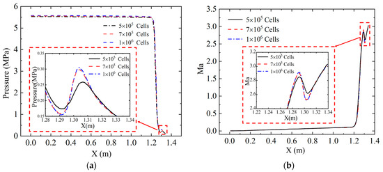
Figure 5.
Grid independence tests. (a) pressure distribution, (b) Mach number distribution.
2.5. Numerical Method Validation
This paper adopted the reference case conducted by Giordano [38] to validate the numerical method and corresponding coupling process. Giordano studied the motion of a cantilever panel under the influence of a shock tube flow using numerical and experimental methods. The calculation settings in the present study are consistent with those in Giordano’s study [38]. According to Giordano, the panel will have an unstable motion at a specific Mach number, which affects the structure of the fluid field. Thus, the estimation of this could validate the fluid–structure interaction method. Figure 6 shows the results of the present numerical at t = 140 μs, t = 280 μs, and t = 420 μs. It can be readily observed that the shock position and plate deformation in the current numerical results exhibit a strong agreement with both Giordano’s experimental and numerical results.
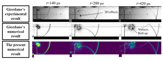
Figure 6.
Validation of the two-way fluid–structure coupling numerical model.
3. Results and Discussion
Section 3.1 describes the internal flow field and structural vibration characteristics of an SRM when the differences between the ground-test and in-flight conditions trigger SRM instability. Section 3.2 presents the coupling relationship between the pressure oscillation and structural vibration during the occurrence of SRM instability. Section 3.3 provides a detailed analysis of the mechanism by which the differences between the ground-test and in-flight conditions trigger SRM instability. In Section 3.4, we conducted an investigation to further study SRM instability under in-flight conditions, specifically focusing on the influence of aerodynamic force frequencies on SRM instability.
3.1. Characteristics of SRM Instability
When operating, the mass flow of gas produced by the burning propellant in a cylindrical-grain motor continuously increases; the thrust and speed of the rocket increase accordingly. As speed increases, shock wave intensity rises, enhancing the aerodynamic heating effects and leading to an increase in SRM casing temperature. The motor consequently experiences continuously shifting aerodynamic conditions, resulting in a substantial variation in the production of aerodynamic heat on the motor casing. To highlight the effect of the aerodynamic heating on an in-flight motor, three flight conditions (corresponding to scenarios T1, T2, and T3) are sketched in Figure 7, with their casing average temperatures at different flight Mach numbers. As its flight Mach number increases, the frontal bow shock is strengthened, leading to a rise in the near-wall fluid temperature and therefore a rise in casing temperature. The attack angle of the solid rocket is 0°, and the atmospheric temperature is 250 K. When the casing average temperature is obtained numerically, the elastic modulus of the casing material could be calculated, as given in Table 4 (Tc is the casing average temperature). Before delving into any of the instability issues within the SRM, it is essential to establish an initial steady state to lay the groundwork for subsequent discussions. In this overall steady state, the fluctuation in both thrust and combustor pressure is only 1/10,000 of their respective average values. The moment when this steady state is achieved is defined as t = 0. This pre-determined overall steady state (all the external flow, the internal flow, and the structures are steady in each scenario) is hereafter named the base state for convenience.
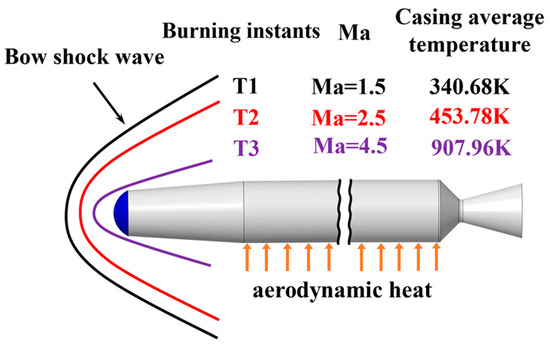
Figure 7.
Schematic of the bow shocks and casing temperature in scenarios T1, T2, and T3.
Table 4.
Casing average temperatures and the corresponding elastic modulus.
In an actual flight, SRMs may subject to oscillatory aerodynamic forces. To take this sort of oscillatory aerodynamic force into account, a continuous aerodynamic force is uniformly imparted on the outer side of the motor casing after the base state is obtained, acting as a surface drag. This aerodynamic force is defined in a sinusoidal form [39,40],
where fp is the frequency of this aerodynamic force. At the moment of t = 0, this aerodynamic force is introduced. The aerodynamic force frequencies in T1, T2, and T3 are set as equal to those for the first-order acoustic frequency of the in-flight SRM, as shown in Table 5. The acoustic modal module of the commercial software ANSYS is used to calculate the first- and second-order audio frequency. The expansion part of the nozzle is excluded in the mode calculation.
Fa = 1000 N + 500 × sin(2πfpt) N
Table 5.
The first two orders of the acoustic frequencies of the combustor.
At t = 0, a sudden mass flux pulse is also imparted on the very head end of the combustion chamber to trigger initial pressure fluctuations resembling those induced by the impact of the detachment of large chunks of propellant. The mass flux magnitude is named as the pulse intensity in this study.
Cases with different aerodynamic loads (different in both the force and heat) but with the same pulse intensities and durations are studied, as shown in Table 6. In the following, the in-flight motor of scenario T1 will be referred to as CaseT1-1 and the ground-test motor of scenario T1 will be referred to as CaseT1-2, the same rule of nomenclature applies to all the other cases.
Table 6.
Cases for in-flight and ground-test SRM simulations.
To better characterize the thrust oscillation characteristics, dimensionless thrust was adopted in this paper. F* is defined as F′/F0, where F′ is the transient thrust and F0 is the steady thrust at the moment t = 0 (i.e., at the base state). The thrust is equal to the axial component of the pressure difference between the internal and external surfaces of the SRM. Figure 8 compares the variations of the dimensionless thrust F* of the cases specified in Table 6. As can be easily detected, in scenario T1, which corresponds to 9/10 of the initial propellant thickness, the thrust variation of the in-flight case (CaseT1-1) is almost identical to that of the ground-test case (CaseT1-2). In T2, which corresponds to 1/2 of the initial propellant thickness, a large difference is shown between the thrust oscillation of the in-flight (CaseT2-1) and ground-test (CaseT2-2) cases. In T3, which corresponds to 1/10 of the initial propellant thickness, identical thrust oscillations for the two cases (CaseT3-1 and CaseT3-2) are obtained again. In scenarios T1 and T3, the thrusts in both the in-flight and ground tests oscillate intensely within 0.005 s after the head-end pulse is triggered but they decay rapidly and return to their base state value after 0.012 s. The peak values of the thrust reach 107% and 112% of the base states for T1 and T3, respectively. In scenario T2, the thrust peak of the in-flight case (CaseT2-1) reaches 115% of the base state. After the initial large-amplitude oscillation, the thrust decays to a limit cycle oscillation [41] with an amplitude of 5% of the base state after 0.01 s. In contrast, the thrust of the ground-test case (CaseT2-2) decays to its base state in a similar way to that in T1 and T3. This indicates that when stimulated by the detachment of a large chunk of propellant (referred to as “pulse” in the subsequent text), only the in-flight T2 state exhibits SRM instability, whereas the T1 and T3 states, as well as the T2 state during the ground test, remain stable. It can be inferred that the differences between in-flight and ground-test conditions are the main cause of this phenomenon.
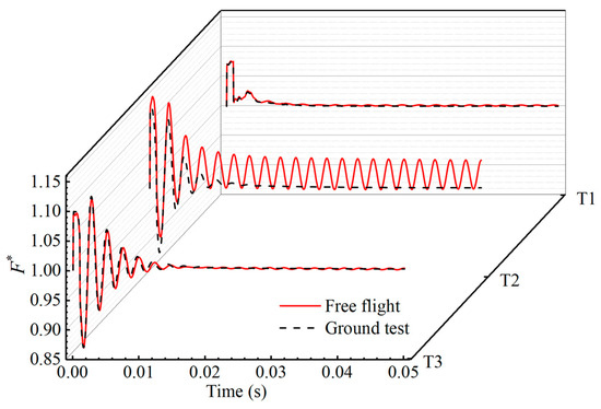
Figure 8.
Temporal variation of thrust oscillation at three burning instants.
The histories of the dimensionless pressure P* (of the cases in Table 6) at three locations, viz., the head end, middle position, and nozzle end of the motor chamber centerline, are shown in Figure 9. Similarly, P* is define as P′/P0, where P′ is the transient pressure and P0 is the base state pressure at t = 0. For all the cases, large-amplitude pressure oscillations are excited immediately by the head-end pulse. In each scenario (take T2 in Figure 9a–c for example), the pulse causes pressure oscillation more intensely at the head end (Figure 9a) and nozzle end (Figure 9c) than at the middle position (Figure 9b). When comparing the pressure oscillation histories in T1, T2, and T3 at each location (take the head end in Figure 9a for example), a salient feature is found where the cases of T1 and T2 during in-flight conditions keep their continuous limit cycle pressure oscillation. In particular, burning rate fluctuations may result in the large-amplitude limit cycle pressure oscillation of the in-flight motor in scenario T2 (CaseT2-1). In this study, the formula used to calculate the combustion rate is expressed as:
where r is burning rate of propellant, P is combustion chamber pressure, and a and n are empirical constants.
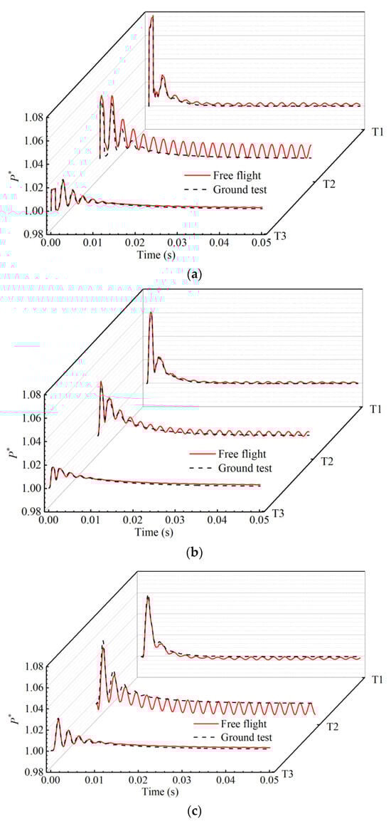
Figure 9.
Temporal variation in pressure oscillation in scenarios T1, T2, and T3. (a) head end, (b) middle position, (c) nozzle end.
Generally, the radial vibration has little effect on the SRM stability due to its small vibration amplitude. Thus, the radial vibration of structure is ignored in this paper. The histories of casing axial vibration at the head end, middle position, and nozzle end are presented by recording the displacement, as shown in Figure 10. The monitoring points on the casing are in an equilibrium position and their initial displacement is zero at t = 0. Due to the existence of the fixed constraints of the test frames in the ground test, steady states are kept at the head end, the middle position, and the nozzle end of the casing. In contrast, under in-flight conditions, the vibration of the casing gradually amplifies and finally maintains a limit cycle vibration in scenario T2, with the maximum value occurring in the nozzle end (Figure 10c). Nevertheless, in scenarios T1 and T3, the casings of the in-flight motors exhibit minimal vibration and remain closely aligned with the base state at t = 0.
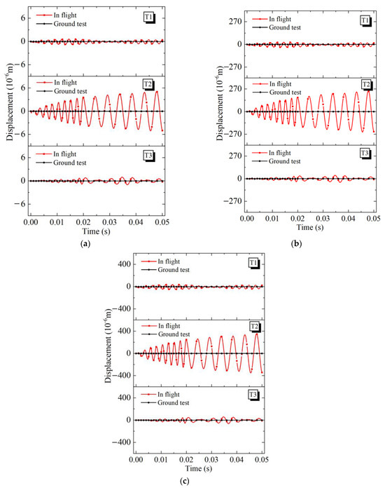
Figure 10.
Temporal variation of axial casing vibration in scenarios T1, T2, and T3. (a) head end, (b) middle position, (c) nozzle end.
The histories of insulation layer axial vibration at the head end, middle position, and nozzle end are presented by recording the displacement, as shown in Figure 11. The monitoring points on the insulation layer are initially at equilibrium with zero displacement at t = 0. Observations indicate that, following the pulse, the insulation layer head ends of the ground-test motors exhibit high-frequency vibrations with low amplitude (as shown in Figure 11a). Subsequently, these vibrations quickly decay and the insulation layer head end returns to its original steady state. Comparing the vibration histories of the three scenarios, it is found that the vibration of the insulation layer gradually amplifies and eventually maintains a limit cycle vibration only in the in-flight motor T2. The maximum value occurs in the nozzle end (Figure 11c).
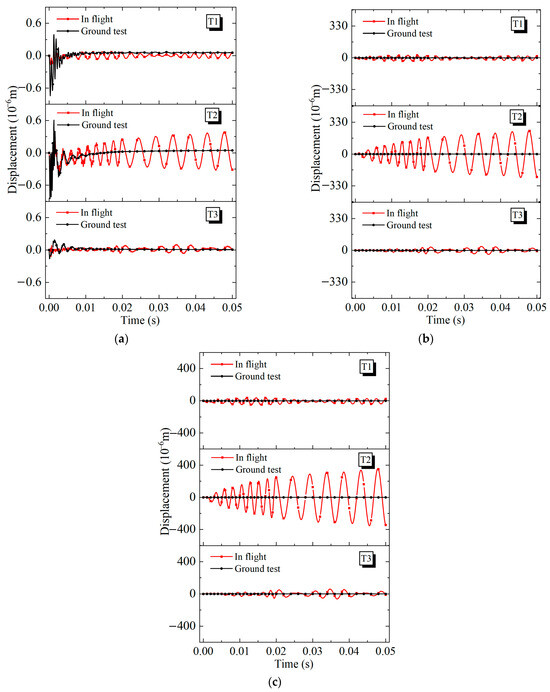
Figure 11.
Temporal variation of axial insulation layer vibration in scenarios T1, T2, and T3. (a) head end, (b) middle position, (c) nozzle end.
The histories of the propellant axial vibration at the head end, middle position, and nozzle end are presented by recording the displacement, as shown in Figure 12. The monitoring points on the propellant are initially in an equilibrium position with zero displacement at t = 0. It is seen that, at the initial stage after the motor is suddenly pulsed, a high-frequency vibration is immediately excited at the head end of the propellant (Figure 12a). Then, the propellant head-end vibration quickly decays and recovers its original steady state. It is found that the propellant vibration of the in-flight motor in scenario T2 gradually amplifies and eventually maintains a limit cycle in the middle position (Figure 12b) and nozzle end (Figure 12c), with the maximum value occurring in the nozzle end (Figure 12c). Thus, it can be speculated that the sustained vibrations in the SRM casing, insulation layer, and propellant during the in-flight T2 state are all caused by the coupling effects of propellant regression and the differences between the in-flight and ground-test conditions.
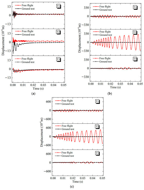
Figure 12.
Temporal variation of axial propellant vibration in scenarios T1, T2, and T3. (a) head end, (b) middle position, (c) nozzle end.
The above results indicate that under in-flight conditions, pulse excitation induces structural vibrations in the SRMs that were not observed in ground-test conditions. The most severe instability occurs in scenario T2. During this condition, the combustion surface is retreated to 1/2. When faced with a pulse excitation, the pressure oscillations and structural vibrations continuously amplify and ultimately develop into limit-cycle-type behaviors. Comparing the oscillation curves at different positions within the SRMs, it can be seen that the oscillation amplitude gradually increases from the head end to the nozzle end when the SRM experiences instability during flight. By comparing the structural vibrations of the casing (Figure 10b,c), insulation layer (Figure 11b,c), and propellant (Figure 12b,c), it becomes evident that the overall structural vibration of the SRM exhibits an increasing trend from the outside to the inside. This indicates that after the initial pressure peak induced by the pulse excitation, sustained structural vibrations and pressure oscillations can only occur when the aerodynamic effects are transmitted to the structure and subsequently propagated to the flow field. Without continuous energy supply from aerodynamic forces (such as in ground test), the flow field and structure cannot maintain sustained oscillations and vibrations.
3.2. Coupling Characteristics of Pressure Oscillation and Structural Vibration
The first two orders of acoustic natural frequencies of the combustion chamber in scenarios T1, T2, and T3 are determined numerically (by neglecting the expansion section of the nozzle), as listed in Table 5. Additionally, because of the minor role played by those higher-than-two-order acoustic modes, they have been neglected in the discussion of this article. Figure 13 shows the pressure variations of the combustion chamber for CaseT2-1 after the mass flux pulse. The period being illustrated spans from t0 = 0.001 s (at the end of the pulse duration) to t0 + 45Δt (where Δt = 5 × 10⁻⁵ s). Clearly seen is that there are pressure waves moving back and forth between the head of the chamber end and the nozzle end; the oscillating frequency of the pressure wave is found to be approximately equal to the first-order acoustic mode frequency.
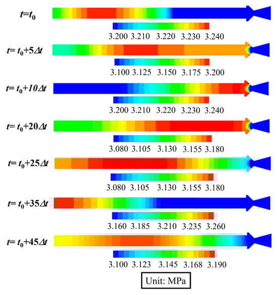
Figure 13.
Temporal variation of pressure contours from t0 to t0 + 45Δt of CaseT2-1.
As shown in Figure 14, the pressure (P) and axial structural accelerations (A) of the propellant surface and casing at the middle position of the SRM is recorded. The structural acceleration within 0.005 s exhibits highly nonlinearity. After 0.005 s, the pressure oscillations and structural vibrations in the ground-test conditions quickly disappear, whereas under in-flight conditions, they develop into limit cycle behaviors. In both ground-test and in-flight conditions, the frequency of pressure oscillations excited by the pulse is nearly the same as the first-order acoustic frequency. This is because during the ground test, there are constraints and no periodic aerodynamic loads exerted on the SRM. As a result, the pressure oscillation and structural vibration quickly decrease and the SRM returns to a stable state. During flight conditions, the propellant and casing are subjected to continuous oscillating internal flow field pressures, while the casing experiences periodic aerodynamic forces, resulting in structural vibrations. Meanwhile, the frequencies of pressure oscillations, structural vibrations, and aerodynamic force are highly similar to each other. This indicates that resonance occurs between the periodic aerodynamic forces, the structure of the SRM, and the internal flow field. Therefore, a detailed investigation into the resonance mechanism between aerodynamic forces, the structure of the SRM, and the internal flow field is conducted in the next section.
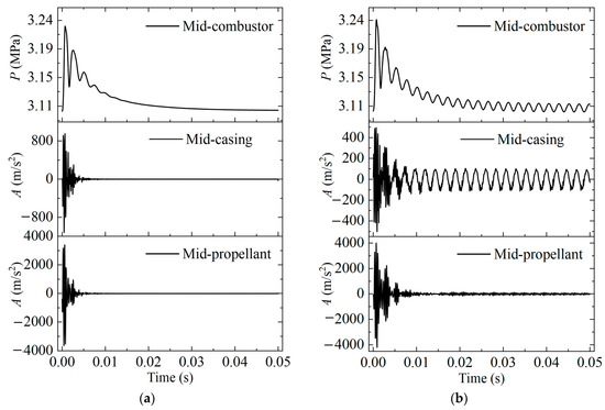
Figure 14.
The response of casing and propellant to the pressure wave. (a) ground test in scenario T2, (b) flight in scenario T2.
3.3. Effects of Aerodynamic Heating and Fixed Constraints on Structural Natural Frequency
Greatrix and Harris [28,29,30] argued that severe SRM instabilities are caused by the coupling of structural vibrations and acoustic oscillations. Thus, the investigation of the relationship between the natural frequencies of the structure and acoustics is of great significance to reveal the mechanism behind SRM instability. As mentioned earlier in Figure 7, the aerodynamic heating causes a sharp decrease in the casing’s elastic modulus, as observed in Table 4. Consequently, the aerodynamic heating can significantly alter the structural natural frequency of the SRM. Moreover, because of the different ways of constraining the SRM, the structural natural frequency of the in-flight SRM can be greatly difference from that of the ground-test SRM. To investigate the structural natural frequency difference between the in-flight SRM and ground-test SRM, the effects of aerodynamic heating and constraints are discussed in this section. Figure 15 shows the frequencies of the first fifty orders of the structural mode for motors in both the in-flight and ground-test cases in scenarios T1, T2, and T3. For comparison, the first two orders of the acoustic mode (given in Table 5) are depicted as the two horizontal dashed lines. It is seen that the structural natural frequencies of the ground-test SRM in each scenario are higher than those of the in-flight SRM due to the fixed constraints used. In scenario T1, the coincidence between the 44th-order structural natural frequency and the 2nd-order acoustic frequency of the ground-test SRM indicates that resonance conditions are present. In scenario T2, the 14th-order structural natural frequency coincides with the 1st-order acoustic frequency of the in-flight case, again indicating the presence of resonance conditions. Other than these two, no coincidence between the structural and the acoustic frequencies is found. This explains the pressure oscillations and the structural vibrations in Section 3.1.
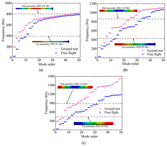
Figure 15.
The natural frequencies of the structural and acoustic modes of the three burning instants, (a) T1, (b) T2, and (c) T3.
Quantitatively, an instability factor Φ is constructed to demonstrate the possibility of resonance of the in-flight SRM. The factor Φ is defined as follows:
where fstructure is the structural frequency and f1st acoustic is the first-order acoustic frequency. Typically, dominant in the acoustic oscillation is the first-order acoustic oscillation. Moreover, high-order acoustic oscillation is hard to excite and does not dominate. At the same time, due to the limitations of the article’s length, we did not delve into its study. Thus, the factor Φ in this paper is only related to the first-order acoustic frequency.
Examining the scenarios T1, T2, and T3 during the in-flight conditions, the values of Φ are shown in Figure 16, according to which, a threshold value of Φ = 0.0027 (within the scope of this study, the Φ is qualitatively set at 0.0027) is found, and this value occurs in T2. As demonstrated in Section 3.1, the in-flight SRMs in scenarios T1 and T3 quickly return to their stable states or exhibit slight oscillations after being excited by the pulse. This indicates that during these moments, SRM instability does not occur. In the contrast, the in-flight SRMs at T2 oscillate severely. Therefore, the factor Φ can serve as an indicator of the SRM operating instability. When the value of Φ falls in the range 0–0.0027, SRM instability may occur. Due to the sample size of the SRM instability phenomenon being small, there is still doubt regarding the exact threshold value of the instability factor Φ. However, it is important to note that the instability parameter Φ still has a relatively high theoretical value.
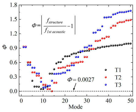
Figure 16.
Instability factor Φ of the in-flight SRMs in different scenarios.
3.4. Effect of Aerodynamic Force Frequency on SRM Instability
Due to the presence of aerodynamic noise at the various frequencies encountered by the in-flight SRM and the unclear impact of aerodynamic force frequencies on SRM instability, this section will investigate the relationship between aerodynamic force frequencies and SRM instability.
To further investigate the phenomenon of SRM instability under in-flight conditions, aerodynamic forces with frequencies fp = 200 Hz, 430 Hz (omit the number after the decimal point of 430.29 Hz), and 600 Hz are applied to the in-flight SRM in scenario T2 (Tc = 453.78 K). As shown in Table 7, the condition with aerodynamic forces applied at 200 Hz is referred to as Case T2-3, whereas the condition with aerodynamic forces applied at 600 Hz is referred to as Case T2-4. The amplitudes of the aerodynamic forces and the strength of the mass flux pulse are the same as those introduced in Section 3.1.
Table 7.
Cases with different aerodynamic force frequencies.
The pressure oscillations of CaseT2-1, CaseT2-3, and CaseT2-4 are also monitored at the SRM head end, middle position, and nozzle end, as shown in Figure 17. At each of these three positions, CaseT2-3 (fp = 200 Hz) and CaseT2-4 (fp = 600 Hz) quickly recover their steady state after 0.01 s. The pressure oscillations in CaseT2-1 (fp = 430 Hz), however, maintain persistent limit cycles. This indicates that aerodynamic forces at the same frequency as the first-order acoustic mode can destabilize an SRM, which satisfies the SRM instability condition (0 ≤ Φ ≤ 0.0027), while aerodynamic forces at other frequencies are unable to induce sustained pressure oscillations. This also suggests that due to the lack of resonance between the aerodynamic force, structure, and acoustic field, other frequencies of aerodynamic forces have a minimal impact on the internal flow field.
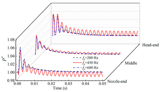
Figure 17.
Temporal variation of pressure oscillation for fp = 200 Hz, fp = 430 Hz, and fp = 600 Hz.
The results of Figure 17 are processed using FFT. The frequency spectra of pressure oscillations, as depicted in Figure 17, are illustrated in Figure 18. It is evident that the predominant frequency is 430 Hz, which corresponds to the first-order acoustic frequency. The maximum pressure oscillation amplitude of 22.2 kPa occurs at the head end of the SRM in CaseT2-1 (fp = 430 Hz). In contrast, the maximum pressure oscillation amplitude for CaseT2-3 (fp = 200 Hz) and CaseT2-4 (fp = 600 Hz) is only 9.0 kPa. This indicates that the primary frequency of pressure oscillations in the internal flow field is the resonance frequency (430 Hz) between the acoustic and structure modes. When the frequency of the aerodynamic force tends to be consistent with the first-order acoustic frequency and the natural frequency of the structure (fp = 430 Hz), it indeed amplifies the pressure oscillations of the internal flow field.
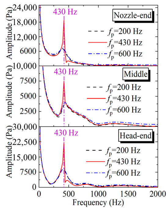
Figure 18.
Frequency spectra of pressure oscillation for fp = 200 Hz, fp = 430 Hz, and fp = 600 Hz.
Figure 19 shows the axial vibrations of the SRM casing, insulation layer, and propellant under the aerodynamic forces of different frequencies. Comparing the vibration histories of the three locations, it is found that the middle position and the nozzle end vibrate with large amplitudes after the pulse. In CaseT2-3 (fp = 200 Hz) and CaseT2-4 (fp = 600 Hz), the vibrations of the casing, insulation layer, and propellant exhibit small amplitudes. This indicates that when the frequency of alternating aerodynamic force is not coupled with the natural frequency of the structure, the structure does not undergo significant vibrations. Conversely, in CaseT2-1 (fp = 430 Hz), the vibrations intensify and eventually reach a sustained limit cycle in all three components (casing, insulation layer, and propellant). The highest amplitudes are observed at the nozzle end. This indicates that when there is a close match between the alternating aerodynamic force and the SRM structural and acoustic natural frequencies, the effect of the aerodynamic force can be efficiently transmitted to the internal flow field through vibrations of the SRM structure. This suggests that the effect of aerodynamic forces can only be effectively transmitted to the internal flow field through vibrations of the SRM structure when there is a close match between the alternating aerodynamic force frequency and the SRM’s structural and acoustic natural frequencies.
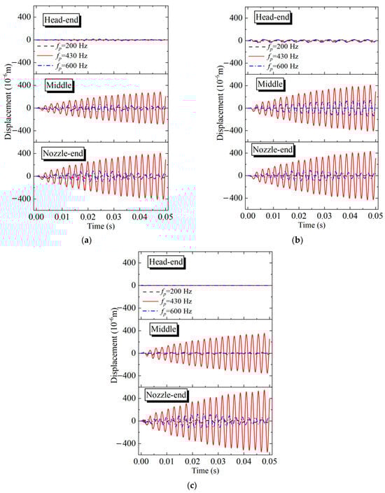
Figure 19.
Axial vibration of casing, insulation layer, and propellant for fp = 200 Hz, fp = 430 Hz, and fp = 600 Hz. (a) casing, (b) insulation layer, (c) propellant.
Again, FFT of the axial vibrations of the casing, insulation layer, and propellant are conducted and shown in Figure 20. For CaseT2-3 (fp = 200 Hz), the axial structural vibration frequency value is 200 Hz. For CaseT2-4 (fp = 600 Hz), the axial structural vibration frequency values are 400 Hz and 600 Hz. Compared with CaseT2-3 and CaseT2-4, CaseT2-1 shows larger axial structural vibration amplitudes in the middle position and at the nozzle end. The axial structural vibration frequency value is 430 Hz. From this, it can be inferred that when the SRM satisfies the instability conditions proposed in Section 3.3, irrespective of the frequency of the aerodynamic forces, the primary frequency of the structural vibrations is the resonance frequency of the SRM in scenario T2.
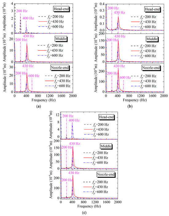
Figure 20.
Spectral analysis of the casing, insulation layer, and propellant axial vibration for fp = 200 Hz, fp = 430 Hz, and fp = 600 Hz. (a) casing, (b) insulation layer, (c) propellant.
The mechanism of the in-flight SRM instability is summarized in Figure 21. In flight, the SRM may be subjected to airflow resistance that can be decomposed into aerodynamic forces at various frequencies. When the frequencies of the aerodynamic force, the structure mode, and the cavity’s acoustic mode coincide with each other, the pressure oscillations excited by the initial pulse and the structural vibrations caused by periodic aerodynamic forces resonate with each other. Finally, the pressure oscillation, thrust oscillations and structural vibrations develop into limit cycle behaviors, ultimately leading to instability in the SRM.
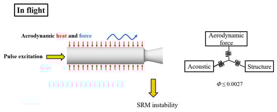
Figure 21.
The mechanism of the aerodynamic–structural–acoustic coupling effects on SRM instability.
4. Conclusions
This paper performed numerical simulations on the mechanism by which SRMs that operate safely during ground tests are prone to failures during free flight. To achieve this, a two-way fluid–structure coupling method was applied to examine the effects of aerodynamic heat, aerodynamic force, and constraints on the stability of the SRM. Drawing from the results of the numerical calculation, the following conclusions are inferred:
- (1)
- The distinctions between the ground-test and in-flight conditions lie in the stronger constraints imposed, as well as the absence of aerodynamic forces and aerodynamic heat in ground tests. This leads to significant differences in the response of an SRM to impulse excitation under in-flight and ground-test conditions. After pulse excitation, compared to ground testing, the combustion chamber pressure, thrust, and structural oscillations of an SRM are significantly amplified during in-flight conditions, eventually leading to limit cycle behaviors.
- (2)
- Under in-flight conditions, the SRM is subjected to weaker constraints and thus structural vibrations are not effectively suppressed. Furthermore, when the natural frequencies of the structure, which are reduced by aerodynamic heating, and the first-order acoustic frequency are increased via a propellant regression approach and reach resonance conditions, the aerodynamic forces caused by airflow resistance are transmitted to the internal flow field through structural vibrations, resulting in the sustained excitation of pressure oscillations in the internal flow field.
- (3)
- The instability factor Φ is proposed to represent the coupling relationship between the structural natural frequency and the first-order acoustic frequency of an SRM. When Φ is within the range 0–0.0027, the SRM is in an unstable state that is highly susceptible to pulse excitation.
- (4)
- The airflow resistance can be decomposed into aerodynamic forces at different frequencies; when the frequencies of aerodynamic forces, first-order acoustic frequency, and structural natural frequency are particularly close, the pressure oscillations and structural vibrations resonate with each other, thus the initial pulse will lead to SRM instability.
Author Contributions
Conceptualization, G.W. and C.L.; methodology, G.W.; software, W.P.; validation, B.Z., C.L. and Z.Y.; formal analysis, C.L.; investigation, G.W.; resources, H.Y.; data curation, Z.Y.; writing—original draft preparation, G.W. writing—review and editing, C.L.; visualization, Z.Y.; supervision, W.P.; project administration, B.Z.; funding acquisition, H.Y. All authors have read and agreed to the published version of the manuscript.
Funding
This research was funded by [Fundamental Research Funds for the Central Universities] grant number [3072022CFJ0203].
Data Availability Statement
The data presented in this study are available on request from the corresponding author.
Conflicts of Interest
The authors declare no conflict of interest.
References
- Blomshield, F.S. Lessons learned in solid rocket combustion instability. In Proceedings of the 43rd AIAA/ASME/SAE/ASEE Joint Propulsion Conference & Exhibit, Cincinnati, OH, USA, 8–11 July 2007. [Google Scholar]
- Zhang, Q.; Wei, Z.J.; Su, W.X.; Li, J.W.; Wang, N.F. Theoretical modeling and numerical study for thrust-oscillation characteristics in solid rocket motors. J. Propuls. Power 2012, 28, 312–322. [Google Scholar] [CrossRef]
- Fabignon, Y.; Dupays, J.; Avalon, G.; Vuillot, F.; Lupoglazoff, N.; Casalis, G.; Prévost, M. Instabilities and pressure oscillations in solid rocket motors. J. Aerosp. Sci. Technol. 2003, 7, 191–200. [Google Scholar] [CrossRef]
- Blomshield, F.S. Historical perspective of combustion instability in motors: Case studies. In Proceedings of the 37th Joint Propulsion Conference and Exhibit, Salt Lake City, UT, USA, 8–11 July 2001. [Google Scholar]
- Blomshield, F.S.; Crump, J.E.; Mathes, H.B.; Stalnaker, R.A.; Beckstead, M.W. Stability testing of full-scale tactical motors. J. Propuls. Power 1997, 13, 349–355. [Google Scholar] [CrossRef]
- Blomshield, F.S.; Stalnaker, R. Pulsed motor firings-pulse amplitude; formulation; enhanced instrumentation. In Proceedings of the 34th AIAA/ASME/SAE/ASEE Joint Propulsion Conference and Exhibit, Cleveland, OH, USA, 13–15 July 1998. [Google Scholar]
- Culick, F.E.C.; Yang, V. Prediction of the stability of unsteady motions in solid propellant rocket motors. AIAA Prog. Astronaut. Aeronaut. 1992, 143, 719–779. [Google Scholar]
- Culick, F.E.C. Nonlinear behavior of acoustic waves in combustion chambers-II. Acta Astronaut. 1976, 3, 735–757. [Google Scholar] [CrossRef]
- Emelyanov, V.N.; Teterina, I.V.; Volkov, K.N.; Garkushev, A.U. Pressure oscillations and instability of working processes in the combustion chambers of solid rocket motors. Acta Astronaut. 2017, 135, 161–171. [Google Scholar] [CrossRef]
- Liu, Y.; Liu, P.; Wang, Z.; Xu, G.; Jin, B. Numerical investigation of mode competition and cooperation on the combustion instability in a non-premixed combustor. Acta Astronaut. 2022, 198, 271–285. [Google Scholar] [CrossRef]
- Ji, S.; Wang, B.; Zhao, D. Numerical analysis on combustion instabilities in end-burning-grain solid rocket motors utilizing pressure-coupled response functions. Aerosp. Sci. Technol. 2020, 98, 105701. [Google Scholar] [CrossRef]
- Narayanaswarni, L.L.; Zinn, B.T.; Daniel, B.R. Investigation of the characteristics of the velocity-coupled response functions of solid propellants. In Proceedings of the 23rd Aerospace Sciences Meeting, Reno, NV, USA, 14–17 January 1985. [Google Scholar]
- Bernardini, M.; Cimini, M.; Stella, F.; Cavallini, E.; Di Mascio, A.; Neri, A.; Martelli, E. Large-eddy simulation of vortex shedding and pressure oscillations in solid rocket motors. AIAA J. 2020, 58, 5191–5201. [Google Scholar] [CrossRef]
- Flandro, G.A.; Jacobs, H.R. Vortex generated sound in cavities. In Proceedings of the Aeroacoustics Conference, Seattle, WA, USA, 15–17 October 1973. [Google Scholar]
- Sun, B.B.; Li, S.P.; Su, W.X.; Li, J.W.; Wang, N.F. Effects of gas temperature on nozzle damping experiments on cold-flow rocket motors. Acta Astronaut. 2016, 126, 18–26. [Google Scholar] [CrossRef]
- Temkin, S.; Dobbins, R.A. Attenuation and dispersion of sound by particulate-relaxation processes. J. Acoust. Soc. Am. 1966, 40, 317–324. [Google Scholar] [CrossRef]
- Fabignon, Y.; Anthoine, J.; Davidenko, D.; Devillers, R.; Dupays, J.; Gueyffier, D.; Hijlkema, J.; Lupoglazoff, N.; Lamet, J.M.; Tessé, L.; et al. Recent advances in research on solid rocket propulsion. J. Aerosp. Lab. 2016, 30, 1–14. [Google Scholar]
- Fowler, J.; Rosenthal, J. Missile vibration environment for solid propellant oscillatory burning. In Proceedings of the 7th Propulsion Joint Specialist Conference, Salt Lake City, UT, USA, 14–18 June 1971. [Google Scholar]
- Hughes, P.M. The Influence of the Elasticity of the Casing and Grain on the Combustion Instability of a Solid Rocket Motor. DREV Memo. 1981, 2588, 81. [Google Scholar]
- Beal, T.R. Dynamic stability of a flexible missile under constant and pulsating thrusts. AIAA J. 1965, 3, 486–494. [Google Scholar] [CrossRef]
- Wu, J.J. On the stability of a free-free beam under axial thrust subjected to directional control. J. Sound Vib. 1975, 43, 45–52. [Google Scholar] [CrossRef]
- Greatrix, D.R. Parametric analysis of combined acceleration effects on solid-propellant combustion. Can. Aeronaut. Space J. 1994, 40, 68–73. [Google Scholar]
- Greatrix, D.R. Combined structural oscillation effects on solid rocket internal ballistics. In Proceedings of the 35th Joint Propulsion Conference and Exhibit, Los Angeles, CA, USA, 20–24 June 1999. [Google Scholar]
- Greatrix, D.R.; Harris, P.G. Structural vibration considerations for solid rocket internal ballistics modeling. In Proceedings of the 36th AIAA/ASME/SAE/ASEE Joint Propulsion Conference and Exhibit, Las Vegas, NV, USA, 24–28 July 2000. [Google Scholar]
- Loncaric, S.; Greatrix, D.R.; Fawaz, Z. Star-grain rocket motor-nonsteady internal ballistics. Aerosp. Sci. Technol. 2004, 8, 47–55. [Google Scholar] [CrossRef]
- Montesano, J.; Behdinan, K.; Greatrix, D.R.; Fawaz, Z. Internal chamber modeling of a solid rocket motor: Effects of coupled structural and acoustic oscillations on combustion. J. Sound Vib. 2008, 311, 20–38. [Google Scholar] [CrossRef]
- Zhang, D.; Cheng, S.; Xu, F.; Hu, Y.; Li, H. Study on nonlinear vibration of simplified solid rocket motor model. Aerosp. Sci. Technol. 2019, 93, 105302. [Google Scholar] [CrossRef]
- Mason, T.D.; Folkman, S.; Behring, M. Thrust oscillations of the Space Shuttle solid rocket Booster motor during static tests. In Proceedings of the 15th Joint Propulsion Conference, Las Vegas, NV, USA, 18–20 June 1979. [Google Scholar]
- Gori, F.; De Stefanis, M.; Worek, W.M.; Minkowycz, W.J. Transient thermal analysis of Vega launcher structures. Appl. Therm. Eng. 2008, 28, 2159–2166. [Google Scholar] [CrossRef]
- Ji, S.; Wang, B. Modeling and analysis of triggering pulse to thermoacoustic instability in an end-burning-grain model solid rocket motor. Aerosp. Sci. Technol. 2019, 95, 105409. [Google Scholar] [CrossRef]
- Version, A.N.Y. 2020R2 User’s Guide; ANSYS, Inc.: Pittsburgh, PA, USA, 2020. [Google Scholar]
- Li, Q.; Liu, P.; He, G. Fluid-solid coupled simulation of the ignition transient of solid rocket motor. Acta Astronaut. 2015, 110, 180–190. [Google Scholar] [CrossRef]
- Bathe, K.J.; Zhang, H.; Wang, M.H. Finite element analysis of incompressible and compressible fluid flows with free surfaces and structural interactions. J. Comput. Struct. 1995, 56, 193–213. [Google Scholar] [CrossRef]
- Xu, G.; Liu, P.; Ao, W.; Wang, Z.; Jin, B. Numerical investigation of thermoacoustic instability caused by small disturbance in a solid rocket motor. Aerosp. Sci. Technol. 2021, 113, 106678. [Google Scholar] [CrossRef]
- Menter, F.R. Two-equation eddy-viscosity turbulence models for engineering applications. AIAA J. 1994, 32, 1598–1605. [Google Scholar] [CrossRef]
- Dowell, E.H.; Hall, K.C. Modeling of fluid-structure interaction. Annu. Rev. Fluid Mech. 2001, 33, 445–490. [Google Scholar] [CrossRef]
- Cook, R.D.; Saunders, H. Concepts and Applications of Finite Element Analysis, 2nd ed.; John Wiley & Sons: New York, NY, USA, 1984. [Google Scholar]
- Giordano, J.; Jourdan, G.; Burtschell, Y.; Medale, M.; Zeitoun, D.E.; Houas, L. Shock wave impacts on deforming panel, an application of fluid-structure interaction. Shock Waves 2005, 14, 103–110. [Google Scholar] [CrossRef]
- Li, S.B.; Wang, Z.G.; Huang, W.; Lei, J.; Xu, S.R. Design and investigation on variable Mach number waverider for a wide-speed range. Aerosp. Sci. Technol. 2018, 76, 291–302. [Google Scholar] [CrossRef]
- Zhang, T.T.; Wang, Z.G.; Huang, W.; Yan, L. Parameterization and optimization of hypersonic-gliding vehicle configurations during conceptual design. Aerosp. Sci. Technol. 2016, 58, 225–234. [Google Scholar] [CrossRef]
- Levine, J.N.; Baum, J.D. A numerical study of nonlinear instability phenomena in solid rocket motors. AIAA J. 1983, 21, 557–564. [Google Scholar] [CrossRef]
Disclaimer/Publisher’s Note: The statements, opinions and data contained in all publications are solely those of the individual author(s) and contributor(s) and not of MDPI and/or the editor(s). MDPI and/or the editor(s) disclaim responsibility for any injury to people or property resulting from any ideas, methods, instructions or products referred to in the content. |
© 2024 by the authors. Licensee MDPI, Basel, Switzerland. This article is an open access article distributed under the terms and conditions of the Creative Commons Attribution (CC BY) license (https://creativecommons.org/licenses/by/4.0/).