Abstract
Heterogeneous multi-UAV systems offer distinct advantages through their complementary and coordinated use of their diverse capabilities. However, this complexity poses significant challenges in task planning, particularly in considering temporal constraints among tasks. As task dependencies evolve from simple linear chains to complex networked associations, uncertainties in flight times can have a substantial impact on the overall schedule. To address these challenges, this study introduces a rapid estimation method that recursively calculates task completion times, derives their probability distributions, and assesses the robustness of the plan. Furthermore, a neighborhood search algorithm guided by dynamic time windows is designed to effectively evaluate the consequences of task insertions, precisely to adjust high-risk tasks, and reduce blindness in enumerative neighborhood exploration. Simulation results demonstrate that the proposed approach effectively accounts for inherent randomness in the problem and exhibits strong adaptability to changes in the problem scale, flight time fluctuations, and variations in time window constraints.
1. Introduction
Heterogeneous multi-UAV systems, by leveraging their diverse capabilities and coordinating complementary functions, offer unmistakable advantages in a wide range of applications. From disaster relief and surveillance to agricultural and forest monitoring, and beyond, they extend their operational scope beyond the limitations inherent in a single UAV, such as voyage duration and resource constraints [1,2]. However, to fully harness these benefits, meticulous task planning is essential as the highest-level strategy for deployments. This planning entails optimizing executable solutions that align with specific task requirements and the capabilities of each unit [3,4,5].
Despite the advantages of heterogeneous multi-UAV systems, effective deployment hinges on managing inevitable uncertainties during task execution. The uncertainties can be mainly categorized into environmental (e.g., meteorological condition changes [6], sudden ground threats [7]), task-related (e.g., task location ambiguities [8,9], resource needs [10], and time window variations [11]), and UAV-specific (e.g., inaccuracies in dynamic models [3,12,13,14], payload performance inconsistencies [3,15], and unexpected UAV failures [16,17]). It is imperative for task planning to comprehensively consider the potential consequences of these uncertainties and accordingly adapt the task plans, thereby minimizing their disruptive effects on the overall task execution.
The flight time of a UAV is calculated based on the estimated task path [18,19] and cruise speed [3,18,19]. It serves as the cornerstone for evaluating the time cost of a task plan. However, due to environmental disturbances and errors in dynamic models [14], resulting in deviations in actual flight time from the predicted values. Such deviations not only affect the current task but also have ripple effects on multiple tasks through task correlation. Increasing flight speeds can mitigate the influence of flight time uncertainties, but this approach has certain limitations. The range of speed increase is constrained, high-speed flight has a limited duration, and it can affect the loiter time [20]. Therefore, it is necessary to consider flight time uncertainties during task planning. Current research mainly employs stochastic programming, Markovian methods, and robust optimization techniques to overcome these challenges.
Stochastic programming employs probability distribution functions to depict uncertain factors. In the literature [3], a two-stage stochastic programming model was adopted to address task planning issues under speed uncertainties. Initially, it filtered plans based on their expected values and then calculated the cost of violations via Monte Carlo simulations. In the literature [13], a fuzzy chance-constrained programming model was used to time uncertainties and formulate multiple plans according to risk appetites. In the literature [21], the expected value and worst-case scenario approaches were investigated in the context of agent speed uncertainties, and it was revealed that the latter usually incur excessively high costs due to their overly cautious nature.
Markovian methods employ a model of an agent’s interaction with its environment to solve sequential decision-making processes under uncertainty. Such methods represent uncertainty in the form of probabilities, usually through transition matrices, and they aim to adjust decisions to maximize cumulative rewards. The literature [22] has focused on the task of moving-target tracking and considered payload confidence and target movement. Transition probabilities were constructed for task paths and observation outcomes, which were then used to solve the optimal observation strategy. By incorporating Markovian principles, the challenges posed by uncertainty in a dynamic and changing environment were addressed.
Robust optimization utilizes uncertainty sets to depict uncertain factors, without relying on probability distribution information. It guarantees the highest feasibility of solutions under the constraints imposed by these sets [10,23]. The literature [24] considered execution time and speed uncertainty by utilizing interval sets to represent task durations. A dominance relationship was designed based on intervals, leading to highly robust solutions, though it was overly conservative. In the literature [25], uncertainty in travel time and resource requirements was addressed using budget sets. This approach integrated a dynamic programming recursive strategy into the task planning model and accurately evaluated the robustness of the obtained solutions through Monte Carlo simulations.
Sequential coupling constraints cause task correlation to evolve from typical linear chains in traditional vehicle routing to more complex networked structures. Due to uncertainty in flight time, both waiting periods and violations resulting from time window constraints can affect task completion time [15]. These effects propagate through the network, thereby impacting subsequent tasks and increasing the overall complexity of the problem. When considering the scale of the solution space, the optimization of task completion counts, and the execution time involves a complex intersection of two well-known NP-Hard problems: the maximum coverage problem and the vehicle routing problem [3,5,26]. Despite having the same task assignment, the uncertainty in flight time can lead to variability in task plans. This obscures the previously well-defined sequential coupling constraints, resulting in a nonlinear expansion of the solution space and, consequently, a significant increase in the computational demands placed on the task planning solving algorithm.
This study addresses the uncertainty in flight time by developing a rapid estimation method for task completion time that considers sequential coupling constraint and time window constraints. This approach enables the rapid evaluation of task plan violation probabilities without the need for Monte Carlo simulations. Meanwhile, a dynamic time window method is introduced to guide neighborhood search algorithms in the adjustment of task assignments by evaluating the impact of task insertion on subsequent tasks. This allows the reinsertion of tasks with high probabilities of violating time window constraints into positions that adhere to the time window, thereby mitigating the blindness of the neighborhood search process.
2. Heterogeneous UAV Collaborative Task Planning Model
2.1. Problem Description
The scenario target is a radar station with its approximate location known. The target damage requirements and task time window have been clearly defined. To simplify calculations, the following assumptions are made:
- The task area is a two-dimensional region, with no consideration given to interfering factors such as terrain obstacles, no-fly zones, or sudden threats.
- Each target involves three types of tasks: reconnaissance, attack, and verification. The number of tasks can be adjusted based on requirements, where each task is executed using a single UAV.
- The task execution duration cannot be ignored, and the width of the task time window is larger than the execution duration.
- UAVs operate at different altitude levels, subject to resource and range limitations. Upon completion of their tasks, they are required to return to their takeoff points.
2.2. Basic Model
Targets: Let be the set of targets, and the target number is . Assuming that the target has tasks, and is the task set of . (reconnaissance (R), attack (A), and verification (V)) can be employed to establish the target-related sequential coupling constraints.
Tasks: The set of tasks is arranged according to the target serial number to form the total set of tasks , and the total number of tasks is . Let be the task in . Given that is the set of execution requirements for task , including the resource requirements , execution duration , capability requirements , and a specific time window . The tasks without specific requirements are subject to an overall completion time .
UAV: Let be the set of heterogeneous UAVs. Let be a set of UAV index parameters including the flight speed , turning radius , included range , number of loads , and capability index . indicates that UAVs can perform the corresponding tasks. Additionally, denotes the task execution sequence of UAV , which is employed to establish the UAV-related sequential coupling constraints.
2.3. Task Correlation Analysis
The target-related and UAV-related sequential coupling constraints are intricately interconnected, forming a complex network of correlations. This intricate relationship extends from the interaction between a single UAV and a single task to all schedules, encompassing task dependencies and interval demands. It is important to note that task correlations are not static but undergo dynamic changes with adjustments in task plans. This section introduces a matrix-based approach for calculating task correlations, specifically involving the coupling correlation matrix, interval time matrix, and sequential coupling correlation matrix.
Target-related sequential coupling correlation matrix : represents the element in the i-th row and j-th column of the matrix. When and , it suggests that can be executed only after the completion of , i.e., is the prior task of , and is the successor task of .
Target-related interval time matrix : The matrix is related to the target-related correlation matrix. When and , it indicates must execute after the completion of with an interval of .
UAV-related sequential coupling correlation matrix : is the element in the i-th row and j-th column of the matrix. indicates that UAV needs to execute task after the completion of , i.e., is the preceding execution task of , and is the subsequent execution task of .
Synthesized sequential coupling correlation matrix : indicates that can affect the execution of . The task meeting is the susceptible task of task , and all tasks meeting constitute the affected susceptible task set of . represents the disjunction operator.
2.4. Task Planning Model
Let the graph model be . Specifically, represents the set of take-off points and tasks, and represents the set of transfer orders between UAV and tasks. Let be the task assignment variable, and indicates that the UAV will travel from to and perform task . The following constraints need to be met:
Equation (3) constrains the allocation relationship; Equation (4) constrains the UAV so that it starts from the takeoff point, returns after completing the task, and the number of UAVs used does not exceed the limit; Equation (5) constrains the resource requirement so that it does not exceed its on-board resource limit; Equation (6) constrains that the UAV, so it can perform the assigned task.
The time-related variables, namely the start time and the completion time of task , are constrained using multiple temporal constraints in the network of correlations. These constraints encompass the target-related sequential coupling constraint, UAV-related sequential coupling constraint, time window constraint, and UAV range constraint.
The complexity of the correlation is reflected in the calculation of the start time and completion time. Taking the start time as an example, as shown in Equations (7)–(9) and Figure 1, the start time is calculated as the maximum of the following relevant values: the completion time of the prior task (denoted as ), the earliest arrival time of the assigned UAV (denoted as ), and the open time of the time window (denoted as ). Additionally, the start time must satisfy the time window constraint presented in Equation (11) and the UAV range constraint given in Equation (12).
In Equation (8), represents the ideal flight time of UAV between and (obtained from the Dubins path [18] and cruise speed ). In Equation (10), denotes the waiting time caused by an unopened time window or incomplete prior tasks. In Equation (12), denotes the departure time of UAV .
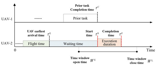
Figure 1.
Calculation diagram of task time.
When considering the uncertainty of flight times, is defined as the flight time for UAV between and . denotes the start time, and denotes the completion time. The completion time of prior tasks is represented as , and the waiting time is denoted as . However, a significant change occurs when certain variables in Equations (7)–(9) transform into continuous stochastic variables, rendering the original solution method obsolete. A new approach, detailed in Section 3, has been devised to address this challenge.
After obtaining the probability distribution of the task start time and completion time, this probability information will be used to assess the likelihood of task breaches. To facilitate this assessment, this paper establishes a task benefit function that incorporates a reward for task completion and a penalty for task breaches. Consequently, as the risk of breaching the time window constraints rises, the value of the task benefit function decreases proportionately.
where represents the probability of breaching the time window constraint, denotes the penalty, and represents the reward. It follows that a higher probability of breaching the time window constraint will result in a lower value of the benefit function. Meanwhile, this paper utilizes the expected task completion time and variance to filter and selects optimal task plans while ensuring equivalent benefits.
3. Rapid Estimation Method for Task Completion Time under Uncertain Flight Times
Under the assumption that flight time follows a normal distribution [3,21], this paper proposes a rapid estimation method for task completion time. By fully considering the sequential coupling constraints among tasks, the proposed method can effectively obtain task completion time and evaluate the robustness of the plan.
3.1. Impact of Uncertain Flight Time on Task Completion Time
The analysis presented in Section 2.4 indicates that both the task’s start time and completion time are influenced by several factors: the earliest arrival time of the assigned UAV, the completion time of prior tasks, and the task time window. The uncertainty inherent in flight time transforms the first two factors into continuous interval random variables. Due to the constraints imposed by the task time window, tasks can be divided into two categories: those completed within the designated timeframe and those that have missed it. Consequently, this section focuses specifically on the calculation of task completion time.
The determination of task completion time involves two key steps. Firstly, it is necessary to find the joint distribution of the two continuous interval random variables representing the completion time of prior tasks and the earliest arrival time of the UAV. Secondly, an analytical expression for the task completion time is derived based on an analysis of the relationship between this joint distribution and the opening and closing times of the task time window. The task completion time is defined as the time when the UAV is ready to depart for the next task, and the sum of the task completion time and flight time yields the earliest possible arrival time at the subsequent destination.
3.2. Maximum Time: Prior Task Completion vs. Earliest UAV Arrival
Denote the completion time of the prior task as and the earliest arrival time of the UAV as . Denote the maximum time between the completion time of the prior task and the earliest arrival time of the assigned UAV as . Denote the probability density function (PDF) for as and its cumulative distribution function (CDF) as .
where is the time variable, is the Gaussian error function, and is the complementary error function. represents the cumulative probability at . The expectation and variance of are given using
Given the distances between tasks and environmental factors, the variance in the earliest arrival time tends to be large. However, since time window constraints could lead to UAV waiting periods, there is smaller variance in the completion time of the prior task. To improve evaluation precision, comparable expected values are assigned to both the arrival time of UAV and completion time of the prior task. More specifically, in Figure 2a, the earliest arrival time of the UAV is illustrated with the purple curve, while the completion time of prior tasks is depicted using the green curve. The blue line traces the PDF of the maximum time . Using Equations (17) and (18), the expected value is 31.63 with a variance of 2.0313. The normal distribution curve is shown as a red dashed line in Figure 2b. Figure 2c compares the CDFs of the maximum time and the normal distribution. Additionally, Figure 2d shows a maximum CDF deviation of 0.0167, confirming a close match between empirical and theoretical data.
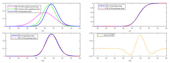
Figure 2.
The calculation result of the maximum time.
3.3. Task Completion Time under Time Windows
The maximum time , a continuous random variable within an interval, has four relative relationships with the task time window: being influenced only by the opening time of the time window (), being influenced only by the closing time of the time window (), being influenced by both the opening and closing time of the time window (), and falling within the time window.
3.3.1. Impact of Time Window Opening Time on Task Completion Time
Considering the open time , must await its commencement before this designated opening time. Conversely, tasks arriving thereafter can commence execution promptly. Given the execution duration , the completion time can be ascertained. The associated PDF and CDF are given using
The task start time must not precede the designated opening time of the time window, thus making the completion time conform to a truncated normal distribution with a lower limit (). When the condition is met, it indicates that the UAV waits before the time window’s commencement, and the corresponding completion time for different points within all coalesce to , resulting in a discontinuity at . The expected value and variance of completion time are given using Equations (22) and (23).
In the context of this study, the maximum time is derived from the simulation results presented in Section 3.2. The analysis focuses on the impact of the time window’s opening time on the completion time . To perform the analysis, the time window is deliberately set to [30, 40]. This allows for the introduction of a probability distribution of to precede the time window’s opening while mitigating any potential influence from the time window’s closing time. Furthermore, to maintain consistency and facilitate comparison, the task execution duration has been fixed at two units throughout the analysis.
In Figure 3a, the black curve represents the PDF of , while the black vertical dashed line indicates the time window’s opening time. The yellow area signifies the scenario in which the UAV arrives early and waits for the time window’s opening, with a cumulative probability of 0.1264. In Figure 3b, the blue curve depicts the PDF of the completion time, which consists of two components: a probabilistic mass point and a curve. Specifically, the former corresponds to the UAV’s arrival before the time window’s opening, with a starting time of 30 and a completion time of 32, yielding a PDF value of 0.1264. The latter is obtained by shifting the distribution after the time window’s opening to the right by two units (task execution duration).
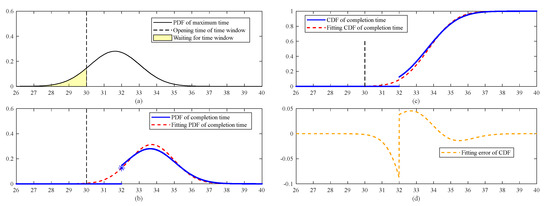
Figure 3.
Task completion times under the influence of the time window’s opening time.
Based on Equations (22) and (23), the expected completion time is calculated to be 33.7196 with a variance of 1.6204. In Figure 3b, the red dashed line depicts the fitting curve corresponding to the normal distribution. Considering the variance of the completion time, the present variance is lower than the variance of the maximum time . Additionally, when the opening time of the time window is delayed to 31, the variance of the completion time further decreases to 1.0733. This indicates that the waiting period of the UAV before the time window commencement diminishes the uncertainty surrounding the task plan. Figure 3c illustrates the CDF before and after fitting, revealing significant fluctuations that are influenced by the time window’s opening time. Specifically, Figure 3d highlights a maximum error of −0.0871 in the fitted CDF, emphasizing the significance of this particular time point.
3.3.2. Impact of Time Window Closing Time on Task Completion Time
Considering the closing time , tasks adhere to constraints and are executed directly if occurs before . Conversely, if occurs after , the task violates the time window constraints, it cannot be executed, and the UAV proceeds to the next task. The PDF and the CDF are provided below.
Due to the influence of task execution duration, there is an overlap between the two sub-functions within the domain in Equation (24). The expected value and variance of completion time are given using Equations (27) and (28), respectively.
is set to the simulation results presented in Section 3.2, and the time window is deliberately set to [20, 33]. This allows for a certain probability distribution of to exist beyond the time window’s closing time while eliminating the influence of the time window’s opening time.
In Figure 4a, the black curve represents the PDF of , while the black vertical dashed line indicates the time window’s closing time. The green area depicts the portion that violates the time window constraints. In Figure 4b, the blue curve illustrates the PDF of the completion time. The increase in probability within the interval (33,35) is attributed to the overlap between two cases: satisfying the time window and violating the time window. For instance, when has a value of 32, the task satisfies the time window and has a completion time of 34. However, when has a value of 34, the task violates the time window, but the completion time remains to be 34. The situation is the same for other time points within the range of (33,35).
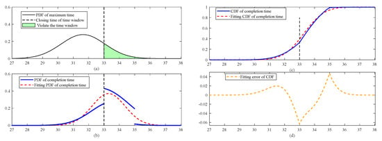
Figure 4.
Task completion times under the influence of the time window’s closing time.
Using Equations (27) and (28), the expected completion time is 33.2936 with a variance of 1.1581. In Figure 4b, the red dashed line represents the fitted normal distribution curve corresponding to these values. In this case, the variance of the completion time has decreased compared to the variance of . However, when the task execution duration is changed to 6, the variance of completion time increases to 2.7697, surpassing that of . This indicates that the distribution of the task completion time has an intricate nature, which is influenced by both the time window’s closing time and the task execution duration. Figure 4c illustrates the CDF both before and after fitting. Notably, the main fluctuations are observed at the two endpoints of the overlapping regions. Specifically, Figure 4d highlights a maximum deviation of −0.0632 in the fitted CDF.
3.3.3. Impact of Time Window Opening and Closing Times on Task Completion Time
When the variance of is relatively large and the time window is narrow, the task completion time is affected by the time window’s opening time and closing time , provided that and are satisfied. The PDF and the CDF are expressed as follows:
The expected value and variance of the completion time, jointly influenced by the time window’s opening and closing time, are given using Equations (32) and (33), respectively.
The maximum time corresponds to the simulation result presented in Section 3.2. To analyze the impact of both the time window’s opening and closing time on the task completion time, a time window of [30, 33] is established.
In Figure 5a, the black curve depicts the PDF of , while the black vertical dashed line indicates the time window. The yellow area depicts the period during which the UAV arrives early and waits for the time window to open. The green area represents the portion that violates the time window constraints. In Figure 5b, the blue curve illustrates the PDF of the completion time, which comprises probability-weighted points and three discontinuous curve segments and is consistent with the preceding analysis.
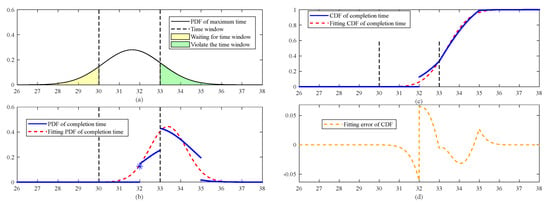
Figure 5.
Task completion times under the influence of the time window’s opening and closing time.
The expected value of the task completion time, derived from Equations (32) and (33), is 33.3832 with a variance of 0.8075. The red dashed line in Figure 5b corresponds to the fitted normal distribution curve. Due to the combined effects of the time window’s opening and closing times, the variance in the completion time has further decreased. Figure 5c illustrates the CDF both before and after fitting. Notably, significant fluctuations are observed at specific time points, particularly at the time window’s opening time (plus the task execution duration) and the endpoints of the overlapping regions. Specifically, Figure 5d highlights a maximum deviation of 0.0649 in the fitted CDF, emphasizing the significance of these fluctuations in the data distribution.
3.4. Earliest Arrival Time for the Next Task
The task completion time is defined as the moment when the UAV commences its subsequent assignment. In deterministic situations, determining the earliest possible arrival time for the following task is straightforward, involving the summation of the task completion time and the flight duration. However, when dealing with uncertain scenarios where both these durations are stochastic and characterized by their own probability distributions, the computation becomes more complex. Specifically, it necessitates the convolution of the PDF of the task completion time with the PDF of the flight time to derive the PDF of the arrival time for the subsequent task (denoted as ).
Due to the influence of time windows, as discussed in Section 3.3, the PDF of the task completion time exhibits irregularity and discontinuity. This irregularity poses a challenge for direct convolution with the flight time PDF due to potential computational expense and inaccuracy. Consequently, this study employs an approximate convolution method that utilizes a normal distribution fitting function for the task completion time. In this section, a comparison is made between this approximate convolution method and direct convolution using the actual distributions of the task completion time. The PDF resulting from the approximate convolution is denoted as , whereas the PDF resulting from direct convolution is denoted as .
Let be the flight time, which is assumed to be independent among different tasks. Following the convolution calculation rules for the normal distribution, is derived by convolving with the task completion time , as shown in Equation (34).
3.4.1. Convolution Calculation of Task Completion Time and Flight Time under the Influence of the Time Window’s Opening Time
In Equation (20), the PDF of the completion time under the influence of the time window’s opening time is mainly divided into two segments. Due to the commutativity property of convolution, the convolution calculation can be independently performed on two distinct segments of the PDF, resulting in two separate functions denoted as and . Subsequently, is obtained by summing the two convolutions.
Based on the simulations presented in Section 3.3.1, let the UAV flight time be . Figure 6a represents the PDF curve for the earliest arrival time of the subsequent task. The blue curve is obtained through piecewise convolution calculations using Equations (35) and (36). Figure 6b represents the CDF curve for the earliest arrival time. Despite the discontinuous nature of the task completion time, the convolution results demonstrate a remarkably smooth profile. The red curve represents the convolution calculation results using the normal distribution fitting function. Notably, both calculation strategies demonstrate excellent approximation performances.
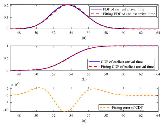
Figure 6.
Earliest arrival time under the influence of time window opening with a flight time variance of 2.
By further analyzing the CDF errors associated with the two calculation strategies, it is observed that the maximum error after the fitting completion time in Section 3.3.1 is −0.0871. Figure 6c demonstrates that the maximum error after the convolution calculations is reduced to −0.0112. Meanwhile, when the flight time variance is expanded to 3, this error is further diminished to −0.0075.
3.4.2. Convolution Calculation of Task Completion Time and Flight Time under the Influence of the Time Window’s Closing Time
The PDF of the completion time under the influence of the time window’s closing time, as represented in Equation (25), is mainly divided into three segments. According to the properties of convolution calculation, it can be transformed into two function segments. Then, convolution calculations are performed separately on these two segments, denoted as and . is obtained by summing the two convolutions.
Based on the simulations in Section 3.3.2, considering the UAV flight time as , Figure 7a depicts the PDF curve for the earliest arrival time of the subsequent task. Figure 7b depicts the CDF curve for the earliest arrival time. The blue curve is derived through piecewise convolution calculations using Equations (37) and (38). The red curve represents the convolution results obtained using the normal distribution fitting function. Both calculation approaches exhibit excellent approximation performance.
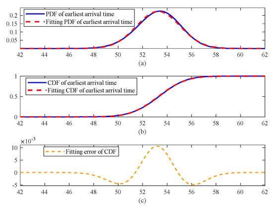
Figure 7.
Earliest arrival time under the influence of time window closing time with a flight time variance of 2.
Further analysis of the CDF errors associated with these two calculation strategies indicates that the maximum error after the fitting completion time in Section 3.3.2 is −0.0632. However, Figure 7c reveals that the maximum error after convolution calculations is reduced to 0.0105. Moreover, as the flight time variance increases to 3, this error is further reduced to 0.0068.
Overall, this indicates that using the normal distribution fitting function for convolution calculations not only simplifies the computational process but also maintains a relatively high degree of solution accuracy. Moreover, the error decreases as the variance of the flight time increases. In the context of this study, the tasks are geographically dispersed, and the flight time between them exhibits significant variance due to environmental factors. In the context of this study, the tasks are geographically dispersed, and the flight time between them exhibits significant variance due to environmental factors. In such cases, directly employing the normal distribution fitting function for convolution calculations is feasible.
3.5. Calculation Process for Task Planning Plan
Based on the aforementioned analysis, the computational process and pseudocode are given below, with specific details provided in Algorithm 1.
- Calculate the completion time of the prior task and the earliest arrival time of the UAV .
- Compute the maximum time according to Equations (17) and (18).
- Determine the relative situation of the maximum time with the time window.
- If and , calculate the task completion time using Equations (32) and (33).
- If , calculate the task completion time using Equations (22) and (23).
- If , calculate the task completion time using Equations (27) and (28).
- In all other cases, the task completion time is , .
| Algorithm 1: Task completion time calculation | |
| Input: Task assignment | |
| Output: Task completion time | |
| 1 | For each task (from 1 to ), perform the following steps: |
| 2 | Calculate the completion time of the prior task |
| 3 | Calculate the earliest arrival time of assigned UAV |
| 4 | Compute the maximum time based on and according to Equations (17) and (18) |
| 5 | Analyze and time window , and execute corresponding steps based on conditions: |
| 6 | If and , calculate completion time according to Equations (32) and (33) |
| 7 | If , calculate completion time according to Equations (22) and (23) |
| 8 | If , calculate completion time according to Equations (27) and (28) |
| 9 | Otherwise, set completion time , |
| 10 | Return the completion times of all tasks |
4. Neighborhood Search Hybrid Evolutionary Algorithm for Uncertain Flight Time
In situations where the flight time is uncertain, task completion time transforms from a specific point to a continuous probability distribution within an interval. Consequently, the actual task completion time may fluctuate within a certain range, and this can lead to variations in the execution outcomes even for the same task assignment, significantly expanding the solution space, and increasing the coordination complexity for temporally coupled tasks. To accurately evaluate the performance of task plans under flight time fluctuations, it is necessary to introduce additional optimization objective functions. However, the increase in optimization objectives will also lead to a higher pressure on solution screening [27]. The task planning problem with uncertain flight time puts forward higher demands on the performance of solution algorithms.
To overcome this challenge, this paper designs a hybrid evolutionary algorithm based on neighborhood search. This algorithm adopts an evolutionary algorithm as the fundamental update framework [28] and incorporates neighborhood search to reassign tasks with higher breach probabilities or those affecting task execution in relatively good task plans, thereby enhancing the performance of the task plans. Since the adjustment of a single task in the neighborhood search process may affect multiple tasks, this paper introduces a dynamic time window based on task correlation and temporal constraints. This design allows for precise evaluation of the effects of task adjustments on subsequent tasks, thereby achieving higher computational efficiency in neighborhood search.
4.1. Algorithm Architecture
With an evolutionary algorithm as its fundamental update framework [28], the hybrid evolutionary algorithm incorporates neighborhood search to conduct the main refined search. During the search process, it selects tasks from promising plans using preset operators and optimizes them through insertion operations. By introducing a dynamic time window, the algorithm can respond to task environment changes in real-time, guiding the reinsertion of tasks to optimize the plan. Task selection, sorting, and insertion are adjusted based on time fluctuations, while the selection probability is dynamically updated according to its performance during the calculation. Additionally, a population reset mechanism is periodically triggered to maintain diversity and prevent stagnation in local optima. The detailed pseudocode of the Algorithm 2 is provided below.
| Algorithm 2: Hybrid evolutionary algorithm | |
| Input: Information of Targets, Tasks and UAVs | |
| Output: Task plan | |
| 1 | Population initialization |
| 2 | While (It<ItMax) do |
| 3 | Crossover and mutation: Perform crossover and mutation operations for task assignment |
| 4 | Update repository: Update repository based on the ordered optimization objective |
| 5 | Dynamic time window: Calculate dynamic time window for each task based on task correlation |
| 6 | Neighborhood search: Accurately adjust individuals in the repository utilizing dynamic time windows as guidance |
| 7 | Update selection probability: Update selection probability for task selection, task sorting, and task insertion operators |
| 8 | Population reset: Perform neighborhood search operations on the entire population |
| 9 | EndWhile |
| 10 | Return Best feasible solution |
4.2. Dynamic Time Window
According to Section 2.4, the start time is constrained by multiple temporal constraints. The introduction of a new task can delay the original start time at the insertion point, which subsequently affects other tasks through task correlation, potentially leading to constraint violations. To rapidly determine whether task insertion will cause violations, this study introduces the concept of the dynamic time window.
The dynamic time window, when applied to a specific task plan, is based on the temporal constraints inherent to each individual task. By incorporating task correlations and utilizing backward reasoning, it translates the temporal constraints of associated, affected tasks onto the current task under consideration. This methodology facilitates the determination of the maximum allowable delay for the current task, thereby guaranteeing adherence to the temporal constraints of all tasks without any violations. The dynamic time window for task is denoted as , where its length is represented by and calculated using Equation (39).
where represents the difference between the task start time and time window’s closing time; represents the difference between the task start time and the maximum range of UAV, with denoting the remaining distance of the UAV. The third term represents the duration of the dynamic time window and waiting time of the susceptible task in the UAV-related sequential coupling correlation matrix; the fourth term represents the difference between the dynamic time window and the start time of the susceptible task in the target-related sequential coupling correlation matrix.
Figure 8 illustrates the calculation of dynamic time windows, encompassing five tasks labeled A through E. Tasks A and B, as well as C and D, form two reconnaissance-attack task sequences with a sequential coupling constraint. A new task, E, is to be inserted before task A. The determination of the dynamic time window for task A relies on task correlation, necessitating a reverse calculation from task D. The closure of task D’s time window dictates its latest commencement. According to the sequential coupling, task C must be completed before task D. It reveals that task D commences earlier than the closure of task C’s time window, thus precluding any postponement of task C beyond the start of D. Task B also precedes D, yet it can be delayed until the closure of its time window after accounting for the requisite flight time. Task A must not only precede task B but also ensure a sufficient flight time between A and C. It indicates that the extended flight time between tasks A and C primarily restricts any delays in task A. The purple shaded area represents the dynamic time window for task A, which is narrower than its original time window, reflecting the temporal constraints imposed by its affected susceptible task. Similarly, the dynamic time windows for tasks B, C, and D can be calculated based on their respective constraints.
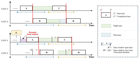
Figure 8.
Schematic of dynamic time window under the influence of subsequent related tasks.
To analyze the impact of inserting a new task, it is sufficient to compare the increase in time after the insertion with the length of the dynamic time window of the original task at the corresponding insertion position. After the new task is inserted, if the start time of the original task at the insertion position still falls within its dynamic time window, then despite changes in the start time of some tasks, the overall task plan will continue to satisfy all temporal constraints. Conversely, if the start time of the original task at the insertion position exceeds the range of its dynamic time window, the insertion of the new task will cause some tasks in the plan to violate constraints. During the neighborhood search operation, giving priority to positions that satisfy the dynamic time window requirements as insertion points for new tasks can minimize interference with the existing task plan.
Considering flight time uncertainty, both the task start time and waiting time described in Equation (39) are transformed into continuous random variables. The obtained dynamic time window also requires precise evaluation through probability, which increases the difficulty in determining the suitability of task insertion. To address this issue, this paper introduces the concept of chance constraints and screens suitable tasks for insertion by adopting a dynamic threshold adjustment strategy.
Specifically, a default threshold is preset for task insertion. When the probability of violating the dynamic time window after a new task is inserted does not exceed the threshold, the task can be considered suitable for insertion. Selecting a higher threshold helps reduce the risk of default but may limit the insertion positions of tasks; selecting a lower threshold facilitates rapid task insertion but may increase the risk of default. Thus, it is necessary to dynamically adjust the threshold during the calculation process, i.e., using a relatively conservative threshold in the initial stage and gradually reducing it when there is no feasible insertion position, thereby balancing the benefits of the solution and the risk of default.
4.3. Neighborhood Search Operation
The neighborhood search operation mainly comprises steps such as task selection, task sorting, task insertion, and probability updating of the operation operators. The selection probabilities of task selection, task sorting, and task insertion operators will be adjusted after a predetermined number of generations [28,29].
- Task Selection:
- a.
- Constraint-violating tasks: select tasks that definitely violate constraints and tasks with a higher probability of violation (in this paper, tasks with a probability of violating time window constraints greater than 0.1 are selected).
- b.
- Predecessor tasks of constraint-violating tasks: Some tasks miss their time windows or have shorter time windows due to the influence of predecessor tasks. In such cases, the predecessor tasks need to be readjusted; otherwise, the tasks cannot be executed.
- c.
- Random selection: randomly select a predetermined number of tasks for reassignment to increase the randomness of the algorithm’s search.
- d.
- Execution duration: Select tasks where the expected change in drone task time after deletion is significant.
- e.
- Path length: select tasks where the change in flight path length after deletion is significant for reassignment and reduction.
- Task Sorting:
Considering the order of task calculation, it is necessary to calculate tasks that satisfy sequential coupling constraints as optional tasks after each task insertion. When there are multiple optional tasks, three sorting operators are used: random sorting, absolute regret sorting, and relative regret sorting [30] to sort the tasks.
- Task Insertion:
- a.
- Time-greedy insertion: select the position where the expected increase in drone time after task insertion is minimal.
- b.
- Path-greedy insertion: according to the C-W strategy [28], select the position where the path increase after task insertion is minimal.
- c.
- Noisy path-greedy insertion: add a certain amount of random noise to the path-greedy insertion operation, with a maximum noise amplitude of 10% of the maximum distance between targets.
- Population Reset Operation:
Considering that the algorithm can simultaneously operate on multiple independent neighborhood actions, it has a fast convergence speed. To avoid the algorithm falling into a local optimal solution, when the optimal solution in the external storage has not been updated for a certain number of iterations, a population reconstruction operation will be triggered. This operation will perform a neighborhood search on the population in hopes of jumping out of the local optimum.
5. Simulation and Analysis
5.1. Simulation Settings
5.1.1. Simulation Scenario Settings
The simulation area ranges 150 150 km, with the take-off point located at [0,0], and the targets are randomly distributed in the area of [10,140] [10,140] km. Considering the task context, the targets will be situated at a considerable distance from the take-off point. Therefore, the minimum distance between the targets and the take-off point is limited to 60 km, and there is a minimum distance limitation between the targets. A time window is required for the attack task, and the number of resources consumed is one; the verification task and the attack task need to be separated by a certain amount of time to avoid the interference of smoke and dust. Table 1 shows the performance data of the UAV.

Table 1.
UAV performance data.
This article selects five scenarios. The first scenario, U-6 T-5 M-15, involves six UAVs, five targets (each encompassing reconnaissance, attack, and assessment tasks), and a total of 15 tasks. The subsequent scenarios are U-6 T-10 M-30, U-9 T-10 M-30, U-9 T-15 M-45, and U-12 T-15 M-45, varying in the number of UAVs, targets, and total tasks. Detailed information on the UAV configurations, target locations, time windows, and optimal task plans (referred to as the original plans, aimed at ensuring the completion of all tasks with the shortest makespan) for the five scenarios can be found in the Table A1 of Appendix A.
To address the flight time uncertainty, two key metrics are introduced: the expected coefficient of the flight time (ratio of expected time to ideal time) and the coefficient of variation (ratio of standard deviation to expected) [25]. Successful task completion earns a reward of 1, whereas violating time window constraints incurs a penalty of −2. To ensure an accurate and intuitive comparative analysis, the study utilizes the full benefit of task completion as the baseline for standardizing benefits across various task plans.
5.1.2. Monte Carlo Method
This article assesses task plan performance using Monte Carlo simulations. Each simulation iteration randomly samples flight times to determine the UAV’s arrival and the resulting benefits. The complete process, including task execution and benefit calculation, is repeated up to MaxIterations times to ensure statistically significant results. The overall performance of the task plan is then evaluated based on the cumulative benefits accrued over all iterations. The calculation pseudocode is provided in Algorithm 3.
| Algorithm 3: Monte Carlo for task plan evaluate | |
| Input: Task plan | |
| Output: Expect benefit | |
| 1 | Initialize Sumbenefit to 0 |
| 2 | For it = 1 to MaxIterations do |
| 3 | Initialize benefit to 0 |
| 4 | For i = 1 to do |
| 5 | Determine the benefit of task |
| 6 | Randomly select CDF value in flight time distribution |
| 7 | Determine flight time by the selected CDF value |
| 8 | Calculate start time of according to Equations (7)–(9) |
| 9 | If meets temporal constraints of Equations (11) and (12) then |
| 10 | benefit = benefit + reward |
| 11 | Else |
| 12 | benefit = benefit + penalty |
| 13 | EndIf |
| 14 | EndFor |
| 15 | Sumbenefit = Sumbenefit + benefit |
| 16 | EndFor |
| 17 | Expbenefit = Sumbenefit / MaxIterations |
| 18 | Return Expbenefit |
5.2. Analysis of the Rapid Estimation Method
5.2.1. Accuracy Analysis
To evaluate the accuracy of the rapid estimation method under flight time uncertainty, this section employs the Monte Carlo method to calculate the original plans in five scenarios. The expected coefficient of flight time is set to 1.1, and the coefficient of variation is set to 0.05. As a result, the actual flight time will fluctuate within a range of 1 to 1.265 times the ideal flight time. The Monte Carlo simulation is conducted with 1000 iterations, and the results are presented as follows: Figure 9 showcases the benefits and makespans of the original plan under Monte Carlo simulation. Specifically, Figure 9a presents the normalized task benefit, whereas Figure 9b illustrates the task completion time. Similarly, Figure 10 and Figure 11 follow the same subfigure structure as Figure 9. Uncertainty in flight time leads to prolonged task durations and reduced benefits, underscoring the plan’s lack of robustness.
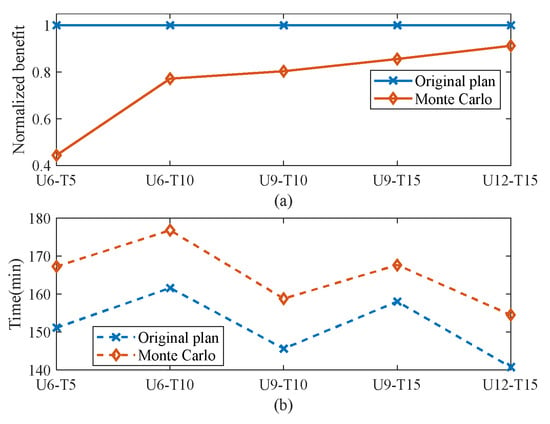
Figure 9.
Comparison between the actual results of the original plan and its estimated results under uncertain scenarios: (a) normalized task benefit and (b) task completion time.
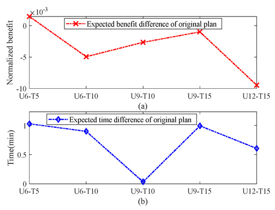
Figure 10.
Difference in plan evaluation results between the proposed rapid estimation method and the Monte Carlo method: (a) normalized task benefit and (b) task completion time.
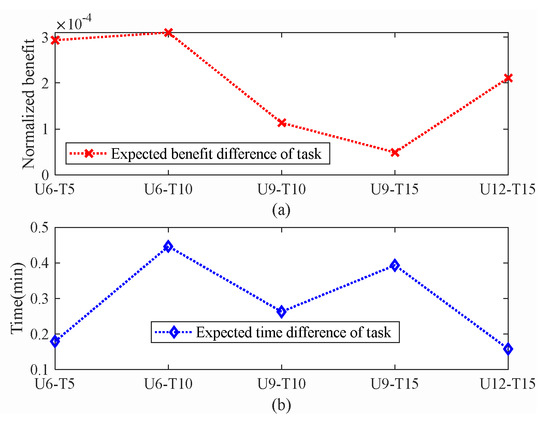
Figure 11.
Difference in task evaluation results between the proposed rapid estimation method and the Monte Carlo method: (a) normalized task benefit and (b) task completion time.
When comparing the rapid estimation method to the Monte Carlo approach in evaluating the overall plan, Figure 10 reveals notable differences. Specifically, the expected time deviation stays under 1 min, and the benefit discrepancy is contained within 0.01. Moving to a more granular level, Figure 11 examines the evaluation errors for individual tasks. Here, the average anticipated error in task completion time does not exceed 0.5 min, while the benefit variance remains within 0.0004. These results indicate that the rapid estimation method closely aligns with the outcomes derived from the Monte Carlo method in terms of task time and benefit assessments.
Finally, Figure 12 illustrates the computation time ratio between the Monte Carlo method and the rapid estimation method. For the Monte Carlo simulations, the scenarios (U6-T5, U6-T10, U9-T10, U9-T15, U12-T15) required 2.7500, 4.9086, 5.5927, 9.2782, and 9.8397 s, respectively. However, the rapid estimation method significantly reduced the computation times for the same scenarios to just 0.0120, 0.0233, 0.0334, 0.0527, and 0.0674 s, respectively. This substantial difference underscores the computational efficiency and reliability of the rapid estimation method, making it a viable and time-saving alternative for accurately assessing task plans, especially in time-sensitive applications.
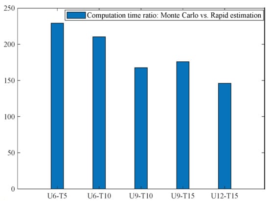
Figure 12.
Ratio of computation time.
5.2.2. Robustness Analysis of Task Plan
This section focuses on the U-9 T-10 M-30 scenario (9 UAVs, 10 targets, and 30 tasks) to further analyze the robustness of the task plan.
In Figure 13, task numbers are enclosed in boxes, with 0 representing the takeoff point. The connecting lines between the boxes denote the transfer of UAV between tasks. Specifically, Tr(A,B) indicates that the expected flight time between targets for a UAV is A, with a variance of B. All time-related values are expressed in minutes. The numbers above the boxes indicate the time windows for each task, while the numbers below the boxes represent the task completion time obtained using the proposed rapid estimation method. Taking the first task 22 of UAV-1 in the figure as an example, the expected flight time is 39.06 with a variance of 3.81. The time window is [0,149], and the expected task completion time is 42.06 with a variance of 3.81.
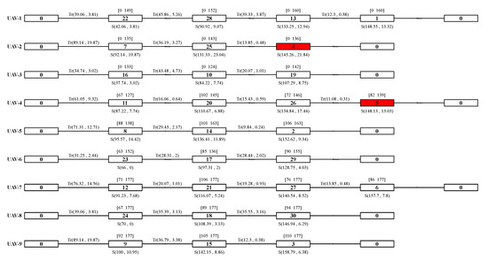
Figure 13.
The original plan under uncertain scenarios.
In Figure 13, tasks 4 and 5 are marked in red to indicate their elevated risk of exceeding the designated time windows. Task 4, in particular, has a 0.97 likelihood of missing its window, primarily due to the preceding tasks—specifically tasks 7 and 25—which leave little room for the UAV to complete the task within the allotted timeframe, thus heightening the chance of a delay. Conversely, task 5 poses an even greater concern with a 0.99 probability of breaching its time window. This elevated risk is not only attributed to its direct predecessor, task 4, but also to the prerequisite tasks performed using the UAV: tasks 11, 20, and 26. The combined impact of these prerequisite tasks pushes the start time dangerously towards the end of the window.
According to Section 3.3, the time window has a significant impact on the variance of the task completion time. When the UAV can arrive before the time window opens, the variance of the task completion time will decrease. If the UAV can ensure early arrival (as shown in task 23), the variance of the task completion time can be reduced to zero, thereby eliminating the uncertainty caused by flight time. In addition, considering the short duration of the tasks in this study, the closing time of the time window further reduces the variance of the task completion time. Without the time window constraint, task 4’s expected completion time variance is 23.52, calculated from task 25’s completion time and flight time. However, due to the time window, this variance is actually reduced to 21.84.
5.3. Verification of Task Planning Method
This section employs the hybrid evolutionary algorithm (hereinafter referred to as the proposed method) to solve the aforementioned scenarios. In the absence of a standard test dataset, the study references similar research to design a set of comparison methods. Based on quartiles, four representative probability values are selected: 0.25, 0.5, 0.75, and 0.99 [14]. Together with the original plan, this results in a total of five different comparison methods, and the Monte Carlo method is used to validate their performance.
These probability values correspond to different estimations of flight time. Specifically, 0.25, as the first quartile of flight time, reflects a shorter time frame and can be considered an optimistic estimate; 0.5 represents the median flight time; 0.75, as the third quartile, reflects a longer time frame and can be viewed as a conservative estimate; and 0.99 represents a near-extreme long duration within the flight time distribution, serving as a highly conservative estimate. By utilizing the inverse cumulative distribution function of flight time, these probability values are converted into deterministic flight times, thus transforming the uncertainty problem into a deterministic one. The CPLEX solver is then employed for problem-solving (with a computation time limit of 7200 s).
5.3.1. Solution Analysis in Single Scenario
This section selects the U-9 T-10 M-30 scenario (nine UAVs, 10 targets, 30 tasks) for analysis. The task benefit and makespan for the five comparison methods and the proposed method are shown in Figure 14. Specifically, Figure 14a presents the task benefit, while Figure 14b illustrates the expected value of the makespan using diamonds and the corresponding variance using horizontal lines.
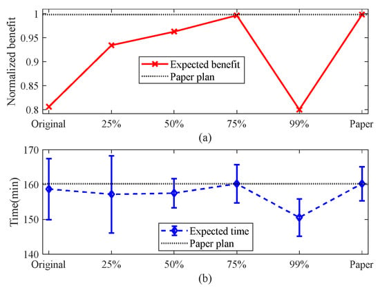
Figure 14.
Comparison of results between the proposed method and the baseline method: (a) normalized task benefit and (b) task completion time.
In the aforementioned simulation, the task plan generated using a probability value of 0.75 achieved the highest benefit. However, as the probability value increased to 0.99, the benefit decreased due to an overly conservative estimation of flight time. This highlights that, while higher probability values can provide more robust time estimates, they may also result in diminished efficiency because of excessive conservatism, especially when UAV resources are scarce. Therefore, practical applications require a careful balancing act when comparing various probability values to mitigate the downsides of over-conservatism. Remarkably, the method introduced in this paper not only maintains execution times on par with the plan utilizing a probability value of 0.75, but also attains a substantial increase in benefit, emphasizing its exceptional flexibility and efficacy.
Figure 15 showcases the task plan devised using our proposed method. All time-related values are expressed in minutes. In contrast to the initial plan, several task execution orders have undergone adjustments. Notably, the sequence of task 4 has been altered to align with time window demands. Despite task 5 maintaining its original order, preceding tasks have become more efficient (for instance, task 11’s completion time dropped from 87.22 to 82.32, and task 20’s from 110.67 to 105.37), indirectly benefiting task 5’s expected completion time. These changes underscore the criticality of considering task interdependencies. As a result, task 4’s breach probability has been eliminated, and task 5’s significantly reduced from 0.99 to just 0.0022, while all other tasks adhere to their respective time windows. Furthermore, the plan’s overall benefit has surged from 0.8062 to 0.9978, markedly bolstering task robustness. This underscores our method’s proficiency in tackling flight time uncertainties.
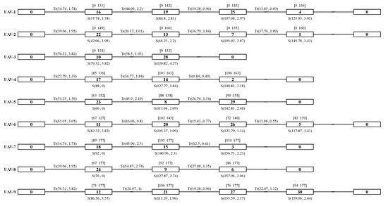
Figure 15.
The task plan generated using the proposed method.
5.3.2. The Impact of Problem Scale
This section solves the remaining four scenarios (U-6 T-5 M-15, U-6 T-10 M-30, U-9 T-15 M-45, U-12 T-15 M-45) and analyzes the performance of the proposed method in solving different scales of scenarios. The calculation results for four scenarios are shown in Figure 16, Figure 17, Figure 18 and Figure 19. Each figure contains two subfigures: subfigure (a) shows the normalized task benefit, while subfigure (b) depicts the task completion time. Due to their structural resemblance across scenarios, detailed depictions are not repeated for each subfigure.
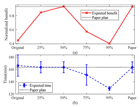
Figure 16.
Comparison of results in scenario U-6 T-5 M-15: (a) normalized task benefit and (b) task completion time.
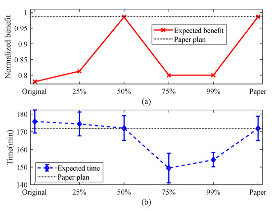
Figure 17.
Comparison of results in scenario U-6 T-10 M-30: (a) normalized task benefit and (b) task completion time.
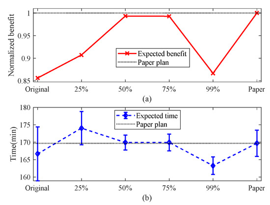
Figure 18.
Comparison of results in scenario U-9 T-15 M-45: (a) normalized task benefit and (b) task completion time.
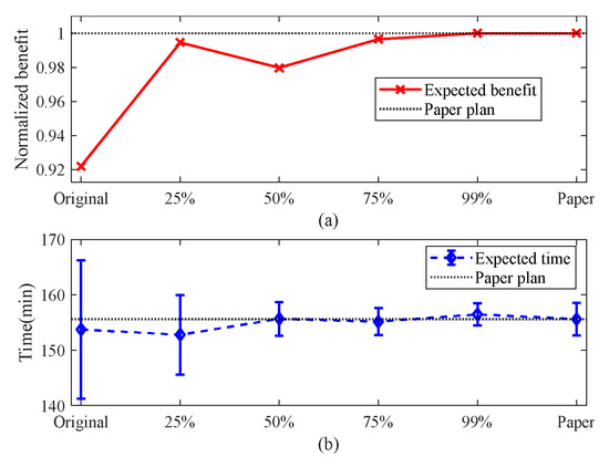
Figure 19.
Comparison of results in scenario U-12 T-15 M-45: (a) normalized task benefit and (b) task completion time.
In the four scenarios, there are significant differences in task plans corresponding to different probability values. Specifically, in the U-6 T-5 M-15 and U-6 T-10 M-30 scenarios, task plans with a probability value of 0.5 perform better, while the benefit decreases significantly when the probability value is 0.75. In the U-9 T-15 M-45 scenario, the performance of probability values 0.5 and 0.75 is comparable, but when the probability value increases to 0.99, the benefit decreases significantly. Finally, in the U-12 T-15 M-45 scenario, the task plan with a probability value of 0.99 performs best. These findings underscore the importance of comprehensively evaluating the task scale and UAV capabilities when addressing uncertainty solely through probability values.
Further analysis reveals that in resource-sufficient situations, relying solely on increasing the estimated flight time may achieve good results in certain scenarios, such as U-12 T-15 M-45, but this also incurs a significant cost increase. In contrast, the method proposed in this paper performs well in various scenarios of different scales. It can generate task plans with benefits at least equivalent to or higher than the best comparison plan, while relatively controlling the growth of time costs. This fully demonstrates the adaptability of the method to different scales of problems.
5.3.3. The Impact of Flight Time
The purpose of this section is to analyze the specific impact of flight time fluctuations on the proposed method. Three parameter sets are considered: an expected coefficient of 1.1 and a coefficient of variation of 0.05 (flight time fluctuates between 1 and 1.265 times the ideal time), an expected coefficient of 1.15 and a coefficient of variation of 0.05 (flight time fluctuates between 1 and 1.323 times the ideal time), and an expected coefficient of 1.2 and a coefficient of variation of 0.06 (flight time fluctuates between 1 and 1.416 times the ideal time). Given the crucial role of flight time consistency in task benefit, the analysis assesses the impact of various parameter sets on task benefit. The calculation results are shown in Figure 20, Figure 21, Figure 22, Figure 23 and Figure 24.
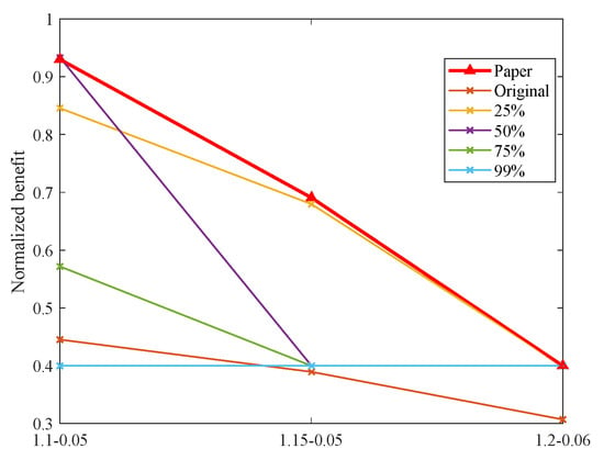
Figure 20.
Comparison of results in scenario U-6 T-5 M-15 with different flight time fluctuations.
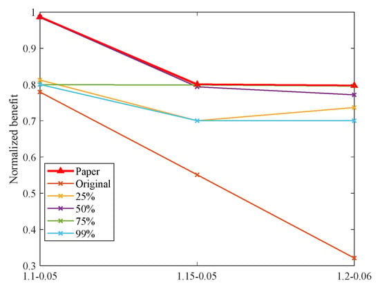
Figure 21.
Comparison of results in scenario U-6 T-10 M-30 with different flight time fluctuations.
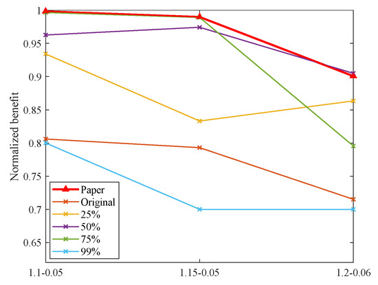
Figure 22.
Comparison of results in scenario U-9 T-10 M-30 with different flight time fluctuations.

Figure 23.
Comparison of results in scenario U-9 T-15 M-45 with different flight time fluctuations.
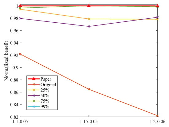
Figure 24.
Comparison of results in scenario U-12 T-15 M-45 with different flight time fluctuations.
In the five scenarios, increasing flight time fluctuations lead to decreased task benefit. Notably, this effect is more pronounced when UAV numbers are limited, as exemplified by conditions like U-6 T-10 M-30. The proposed method consistently outperforms others in terms of maintaining higher benefit. This advantage is due to its thorough consideration of flight time uncertainties during the design process. By swiftly identifying risks of plan breaches and dynamically adjusting task assignments, the method optimizes task benefit across a wide range of flight time variations. Thus, it showcases its adaptability in various operational environments.
5.3.4. The Impact of Time Window
The section delves into the specific impact of time window reduction. The time windows are shortened to 80% and 60% of their original lengths (the opening time remains fixed, while the closing time is adjusted accordingly). The expected coefficient for flight time is set to 1.1 and the coefficient of variation is set to 0.05. The analysis focuses on the impact of different time window settings on task benefit. The calculation results are shown in Figure 25, Figure 26, Figure 27, Figure 28 and Figure 29.
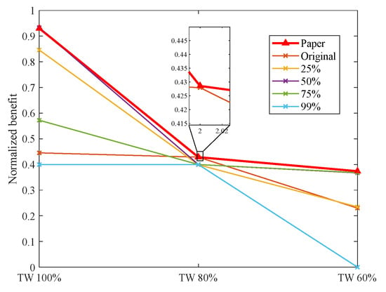
Figure 25.
Comparison of results in scenario U-6 T-5 M-15 with different time window reductions.
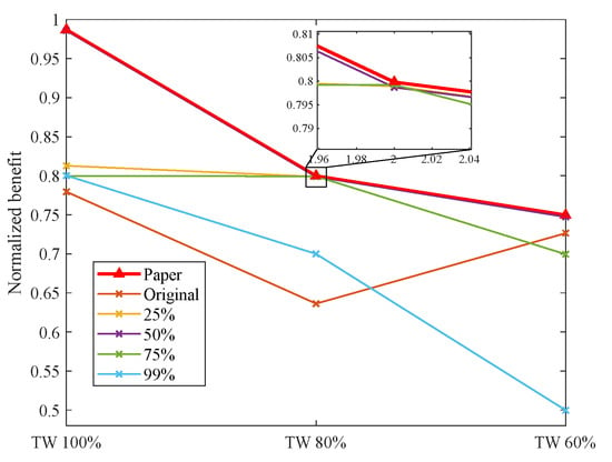
Figure 26.
Comparison of results in scenario U-6 T-10 M-30 with different time window reductions.
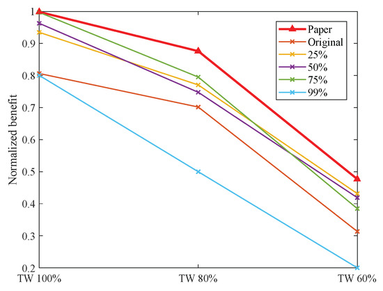
Figure 27.
Comparison of results in scenario U-9 T-10 M-30 with different time window reductions.
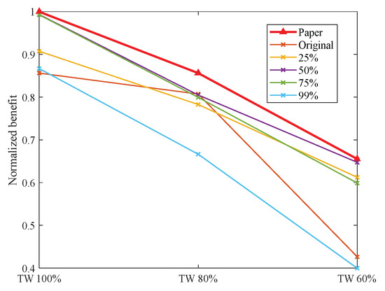
Figure 28.
Comparison of results in scenario U-9 T-15 M-45 with different time window reductions.
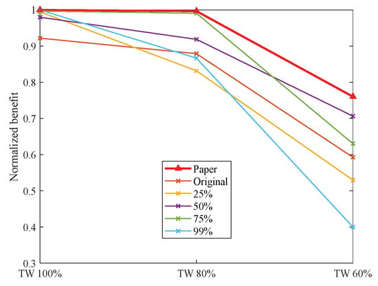
Figure 29.
Comparison of results in scenario U-12 T-15 M-45 with different time window reductions.
Across the five scenarios examined, the shortening of time windows has led to a certain decline in task benefit for various methods. Compared to alternative approaches, the method presented in this paper demonstrates a consistent ability to maintain a higher level of task benefit, particularly exhibiting significant advantages in the three scenarios of U-9 T-10 M-10, U-9 T-15 M-45, and U-12 T-15 M-45.
This notable performance can be primarily attributed to the incorporation of two key strategies in our method: dynamic time windows and dynamic thresholding. As the task time windows shrink, the number of risk-free task insertion positions diminishes. Our method navigates this challenge by guiding neighborhood search operations through dynamic time windows and selectively choosing task insertion positions via dynamic threshold adjustments. This balanced approach between minimizing breach risk and maximizing overall plan benefit enables continuous optimization of the task plan.
6. Conclusions
This paper designs a rapid estimation method for task completion time, considering the uncertainty of flight time. Expressions are derived for task completion time under varying time window constraints, facilitating the recursive computation of task duration based on task correlation. This approach enables swift and precise evaluation of the robustness of task plans, obviating the need for costly numerical simulations.
Leveraging task correlation and temporal constraints, a dynamic time window for tasks is established to efficiently assess how the introduction of a new task affects subsequent ones. The hybrid evolutionary algorithm precisely adjusts task assignments in response to the dynamic time window, reallocating tasks with higher probabilities of violating constraints or negatively impacting task execution, thereby bolstering the resilience of the task plan.
The proposed methodology comprehensively accounts for the stochastic nature of the problem and exhibits strong adaptability to changes in task scale, temporal fluctuations, and time window variations. It eliminates the redundant verification of numerous probability values typically required in comparative methods, attaining robust task plans with minimal increments in time costs and without significantly increasing computational complexity.
In the future, research efforts will explore alternative flight time distributions, including the Gamma distribution, to gauge changes in calculation accuracy and efficiency across diverse scenarios. Studies will also delve into task execution time and its maximum time distribution, elucidating how time window closures affect task completion variance. Furthermore, the integration of adversarial risks such as interference and hacking into UAV models is crucial for understanding their real-world ramifications on task planning and execution.
Author Contributions
Conceptualization, J.W. and G.J.; methodology, J.W.; software, J.W.; validation, J.W., Z.H. and Z.G.; formal analysis, J.W.; investigation, J.W. and G.J.; resources, Z.G.; data curation, J.W.; writing—original draft preparation, J.W. and Z.G.; writing—review and editing, G.J. and Z.H.; visualization, J.W.; supervision, Z.H.; project administration, Z.H.; funding acquisition, G.J. All authors have read and agreed to the published version of the manuscript.
Funding
This research was funded by National Natural Science Foundation of China 61801495.
Data Availability Statement
Data are contained within the article.
Conflicts of Interest
The authors declare no conflict of interest.
Appendix A
There is no suitable standardized test set available for the task planning problem addressed in this paper. This is due to the presence of complex constraints, including sequential coupling, heterogeneous capabilities, time windows, and resource limitations. As a result, existing test sets cannot be directly applied to evaluate the performance of our algorithms. To address this gap, we have designed a comprehensive set of scenarios tailored to our problem domain. Using the CPLEX solver, we have computed benchmark solutions for these scenarios, imposing a computation time limit of 7200 s.
The table included in this paper presents various pieces of information pertinent to the scenarios and their solutions. Specifically, the second column of the table outlines details related to the targets and UAVs involved. The last column of the table showcases the optimal or benchmark solutions obtained for each instance. These solutions encompass assignment relationships and start times. For instance, “1-U1:(31.22)” represents that UAV executes the task at 31.22 min.

Table A1.
Benchmark solutions obtained for five instances.
Table A1.
Benchmark solutions obtained for five instances.
| Configuration | Target | Position (km) | Time Window (min) | Benchmark: Task-UAV and Start Time (min) | ||||
| 6 UAV (2-2-2) 5 Target | 1 | 53 | 33 | 95 | 147 | 1-U1:(31.22) | 2-U3:(138.42) | 3-U5:(148.25) |
| 2 | 126 | 21 | 73 | 147 | 4-U1:(71.23) | 5-U3:(74.23) | 6-U6:(78.23) | |
| 3 | 35 | 136 | 69 | 157 | 7-U2:(70.3) | 8-U4:(73.3) | 9-U5:(77.3) | |
| 4 | 121 | 129 | 89 | 135 | 10-U1:(128.31) | 11-U4:(131.31) | 12-U6:(135.31) | |
| 5 | 83 | 83 | 86 | 146 | 13-U2:(109.08) | 14-U3:(112.08) | 15-U5:(116.09) | |
| Configuration | Target | Position (km) | Time window (min) | Benchmark: Task-UAV and Start Time (min) | ||||
| 6 UAV (2-2-2) 10 Target | 1 | 74 | 32 | 104 | 145 | 1-U1:(40.31) | 2-U4:(104) | 3-U6:(108) |
| 2 | 103 | 76 | 58 | 132 | 4-U1:(69.7) | 5-U4:(72.7) | 6-U6:(76.7) | |
| 3 | 18 | 99 | 54 | 135 | 7-U2:(50.43) | 8-U3:(54) | 9-U5:(58) | |
| 4 | 20 | 78 | 57 | 154 | 10-U2:(64.06) | 11-U3:(67.06) | 12-U5:(71.63) | |
| 5 | 117 | 117 | 118 | 149 | 13-U2:(127.73) | 14-U3:(130.73) | 15-U5:(140.84) | |
| 6 | 137 | 95 | 108 | 149 | 16-U2:(145.6) | 17-U3:(148.6) | 18-U5:(158.72) | |
| 7 | 69 | 67 | 68 | 142 | 19-U1:(90.35) | 20-U3:(96.51) | 21-U5:(103.17) | |
| 8 | 61 | 119 | 113 | 155 | 22-U1:(122.67) | 23-U4:(145.22) | 24-U6:(158.02) | |
| 9 | 65 | 96 | 112 | 152 | 25-U1:(108) | 26-U4:(132.88) | 27-U6:(143.35) | |
| 10 | 48 | 67 | 84 | 151 | 28-U2:(82.11) | 29-U3:(85.11) | 30-U5:(89.67) | |
| Configuration | Target | Position (km) | Time window (min) | Benchmark: Task-UAV and Start Time (min) | ||||
| 9 UAV (3-3-3) 10 Target | 1 | 123 | 18 | 106 | 163 | 1-U1:(133.27) | 2-U5:(136.27) | 3-U9:(142.72) |
| 2 | 118 | 130 | 82 | 139 | 4-U2:(132.65) | 5-U4:(135.65) | 6-U7:(142.12) | |
| 3 | 138 | 85 | 88 | 138 | 7-U2:(81.06) | 8-U5:(88) | 9-U9:(92) | |
| 4 | 22 | 137 | 67 | 127 | 10-U3:(74.16) | 11-U4:(77.16) | 12-U7:(81.16) | |
| 5 | 103 | 28 | 101 | 163 | 13-U1:(119.09) | 14-U5:(122.09) | 15-U9:(128.52) | |
| 6 | 25 | 58 | 85 | 136 | 16-U3:(31.62) | 17-U6:(91.78) | 18-U8:(102.22) | |
| 7 | 58 | 131 | 102 | 145 | 19-U3:(95.43) | 20-U4:(102) | 21-U7:(106) | |
| 8 | 70 | 12 | 63 | 152 | 22-U1:(35.52) | 23-U6:(63) | 24-U8:(67) | |
| 9 | 93 | 133 | 72 | 146 | 25-U2:(117.02) | 26-U4:(120.02) | 27-U7:(126.53) | |
| 10 | 78 | 95 | 90 | 155 | 28-U1:(80.27) | 29-U6:(120.65) | 30-U8:(137.56) | |
| Configuration | Target | Position (km) | Time window (min) | Benchmark: Task-UAV and Start Time (min) | ||||
| 9 UAV (3-3-3) 15 Target | 1 | 38 | 50 | 29 | 135 | 1-U1:(55.85) | 2-U6:(58.85) | 3-U8:(62.85) |
| 2 | 40 | 120 | 53 | 117 | 4-U3:(66.89) | 5-U5:(69.89) | 6-U7:(73.89) | |
| 3 | 67 | 51 | 71 | 127 | 7-U2:(42.11) | 8-U4:(71) | 9-U9:(75) | |
| 4 | 138 | 68 | 109 | 162 | 10-U1:(139.39) | 11-U4:(142.39) | 12-U9:(150.1) | |
| 5 | 45 | 89 | 90 | 138 | 13-U2:(103.96) | 14-U6:(113.69) | 15-U8:(120.61) | |
| 6 | 52 | 66 | 81 | 145 | 16-U1:(42.12) | 17-U6:(81) | 18-U8:(85) | |
| 7 | 14 | 131 | 114 | 160 | 19-U2:(133.07) | 20-U6:(137.57) | 21-U8:(149.71) | |
| 8 | 74 | 86 | 99 | 150 | 22-U2:(86.38) | 23-U6:(99) | 24-U8:(103) | |
| 9 | 70 | 136 | 86 | 156 | 25-U3:(86.89) | 26-U5:(89.89) | 27-U7:(93.9) | |
| 10 | 92 | 99 | 59 | 123 | 28-U2:(72.23) | 29-U5:(110.12) | 30-U7:(118.44) | |
| 11 | 126 | 129 | 81 | 141 | 31-U3:(134.4) | 32-U5:(137.4) | 33-U7:(149.41) | |
| 12 | 99 | 28 | 98 | 159 | 34-U1:(91.31) | 35-U4:(98) | 36-U9:(102) | |
| 13 | 24 | 95 | 43 | 127 | 37-U3:(49.05) | 38-U5:(52.05) | 39-U7:(56.05) | |
| 14 | 112 | 103 | 92 | 146 | 40-U3:(116.62) | 41-U5:(121.29) | 42-U7:(131.65) | |
| 15 | 103 | 76 | 93 | 153 | 43-U1:(118.42) | 44-U4:(121.42) | 45-U9:(129.13) | |
| Configuration | Target | Position (km) | Time window (min) | Benchmark: Task-UAV and Start Time (min) | ||||
| 12 UAV (4-4-4) 15 Target | 1 | 77 | 55 | 90 | 148 | 1-U2:(83.04) | 2-U6:(90) | 3-U9:(94) |
| 2 | 110 | 44 | 111 | 146 | 4-U2:(62.62) | 5-U6:(111) | 6-U9:(115) | |
| 3 | 46 | 74 | 42 | 142 | 7-U3:(43.59) | 8-U7:(46.59) | 9-U12:(50.59) | |
| 4 | 129 | 113 | 73 | 147 | 10-U1:(110.52) | 11-U5:(115.14) | 12-U10:(123.1) | |
| 5 | 97 | 104 | 86 | 146 | 13-U1:(90.86) | 14-U8:(93.86) | 15-U12:(100.98) | |
| 6 | 108 | 80 | 80 | 147 | 16-U1:(74.64) | 17-U8:(80) | 18-U12:(84.76) | |
| 7 | 71 | 100 | 98 | 141 | 19-U3:(72.85) | 20-U7:(98) | 21-U11:(103.25) | |
| 8 | 70 | 21 | 64 | 124 | 22-U1:(36.54) | 23-U6:(64) | 24-U9:(68) | |
| 9 | 117 | 133 | 78 | 139 | 25-U1:(125.19) | 26-U5:(128.19) | 27-U10:(137.76) | |
| 10 | 140 | 40 | 63 | 154 | 28-U4:(72.81) | 29-U5:(75.81) | 30-U9:(133.13) | |
| 11 | 20 | 129 | 94 | 152 | 31-U3:(122.55) | 32-U8:(129.24) | 33-U11:(135.59) | |
| 12 | 93 | 32 | 50 | 137 | 34-U2:(49.18) | 35-U5:(52.18) | 36-U11:(56.18) | |
| 13 | 66 | 74 | 83 | 139 | 37-U3:(56.61) | 38-U7:(83) | 39-U11:(87) | |
| 14 | 75 | 132 | 70 | 142 | 40-U3:(91.99) | 41-U7:(113.9) | 42-U12:(121.79) | |
| 15 | 140 | 75 | 78 | 130 | 43-U4:(93.31) | 44-U5:(96.31) | 45-U10:(100.31) | |
References
- Wu, Y.; Liang, T.; Gou, J.; Tao, C.; Wang, H. Heterogeneous Mission Planning for Multiple UAV Formations via Metaheuristic Algorithms. IEEE Trans. Aerosp. Electron. Syst. 2023, 59, 3924–3940. [Google Scholar] [CrossRef]
- Wu, W.; Xu, J.; Sun, Y. Integrate Assignment of Multiple Heterogeneous Unmanned Aerial Vehicles Performing Dynamic Disaster Inspection and Validation Task with Dubins Path. IEEE Trans. Aerosp. Electron. Syst. 2023, 59, 4018–4032. [Google Scholar] [CrossRef]
- Jia, Z.; Yu, J.; Ai, X.; Xu, X.; Yang, D. Cooperative Multiple Task Assignment Problem with Stochastic Velocities and Time Windows for Heterogeneous Unmanned Aerial Vehicles Using a Genetic Algorithm. Aerosp. Sci. Technol. 2018, 76, 112–125. [Google Scholar] [CrossRef]
- Yao, Z.; Li, M.; Chen, Z.; Zhou, R. Mission Decision-Making Method of Multi-Aircraft Cooperatively Attacking Multi-Target Based on Game Theoretic Framework. Chin. J. Aeronaut. 2016, 29, 1685–1694. [Google Scholar] [CrossRef]
- Eun, Y.; Bang, H. Cooperative Task Assignment/Path Planning of Multiple Unmanned Aerial Vehicles Using Genetic Algorithm. J. Aircr. 2009, 46, 338–343. [Google Scholar] [CrossRef]
- Yomchinda, T.; Horn, J.F.; Langelaan, J.W. Modified Dubins Parameterization for Aircraft Emergency Trajectory Planning. Proc. Inst. Mech. Eng. Part G J. Aerosp. Eng. 2016, 231, 374–393. [Google Scholar] [CrossRef]
- Zhou, W.; Qi, R.; Jiang, B. Mission replanning method of distributed multiple unmanned aerial vehicles for pop-up faults. Control. Decis. 2023, 38, 1373–1385. [Google Scholar]
- Evers, L.; Barros, A.I.; Monsuur, H.; Wagelmans, A. Online Stochastic UAV Mission Planning with Time Windows and Time-Sensitive Targets. Eur. J. Oper. Res. 2014, 238, 348–362. [Google Scholar] [CrossRef]
- Moon, S.; Yang, K.; Gan, S.; Shim, D. Decentralized Information-Theoretic Task Assignment for Searching and Tracking of Moving Targets. In Proceedings of the International Conference on Unmanned Aircraft Systems, Denver, CO, USA, 9–12 June 2015; pp. 1031–1036. [Google Scholar]
- Subramanyam, A.; Repoussis, P.P.; Gounaris, C.E. Robust Optimization of a Broad Class of Heterogeneous Vehicle Routing Problems under Demand Uncertainty. INFORMS J. Comput. 2020, 32, 661–681. [Google Scholar] [CrossRef]
- Zhang, Y.; Baldacci, R.; Sim, M.; Tang, J. Routing Optimization with Time Windows under Uncertainty. Math. Program. 2019, 175, 263–305. [Google Scholar] [CrossRef]
- Cui, J.; Wei, R.; Liu, Z.; Zhou, K. UAV Motion Strategies in Uncertain Dynamic Environments: A Path Planning Method Based on Q-Learning Strategy. Appl. Sci. 2018, 8, 2169. [Google Scholar] [CrossRef]
- Zhang, A.; Yang, M.; Bi, W.; Zhang, B.; Wang, Y. Task allocation of heterogeneous multi-UAV in uncertain environment based on multiple strategies GWO. Acta Aeronaut. Et Astronaut. Sin. 2022, 44, 327115. [Google Scholar]
- Ponda, S.S.; Johnson, L.B.; How, J.P. Distributed Chance-Constrained Task Allocation for Autonomous Multi-Agent Teams. In Proceedings of the American Control Conference, Montreal, QC, Canada, 27–29 June 2012. [Google Scholar]
- Verbeeck, C.; Vansteenwegen, P.; Aghezzaf, E.H. Solving the Stochastic Time-Dependent Orienteering Problem with Time Windows. Eur. J. Oper. Res. 2016, 255, 699–718. [Google Scholar] [CrossRef]
- Dulai, T.; Werner-Stark, Á.; Hangos, K.M. Algorithm for Directing Cooperative Vehicles of a Vehicle Routing Problem for Improving Fault-Tolerance. Optim. Eng. 2017, 19, 239–270. [Google Scholar] [CrossRef]
- Patel, R.; Rudnick-Cohen, E.; Azarm, S.H.; Jeffrey, W. Robust Multi-Uav Route Planning Considering UAV Failure. In Proceedings of the International Conference on Unmanned Aircraft Systems (ICUAS), Atlanta, GA, USA, 11–14 June 2019; pp. 205–212. [Google Scholar]
- Wu, W.; Wang, X.; Cui, N. Fast and Coupled Solution for Cooperative Mission Planning of Multiple Heterogeneous Unmanned Aerial Vehicles. Aerosp. Sci. Technol. 2018, 79, 131–144. [Google Scholar] [CrossRef]
- Wang, G.G.; Chu, H.E.; Mirjalili, S. Three-Dimensional Path Planning for Ucav Using an Improved Bat Algorithm. Aerosp. Sci. Technol. 2016, 49, 231–238. [Google Scholar] [CrossRef]
- Gudmundsson, S. General Aviation Aircraft Design Applied Methods and Procedures; Elsevier: Amsterdam, The Netherlands, 2022. [Google Scholar] [CrossRef]
- Whitbrook, A.; Meng, Q.; Chung, P.W.H. Addressing Robustness in Time-Critical, Distributed, Task Allocation Algorithms. Appl. Intell. 2019, 49, 1–15. [Google Scholar] [CrossRef]
- Campbell, T.; Johnson, L.; How, J. Multiagent Allocation of Markov Decision Process Tasks. In Proceedings of the American Control Conference, Washington, DC, USA, 17–19 June 2013; pp. 2356–2361. [Google Scholar]
- Chen, Y.; Yang, D.; Yu, J. Multi-UAV Task Assignment with Parameter and Time-Sensitive Uncertainties Using Modified Two-Part Wolf Pack Search Algorithm. IEEE Trans. Aerosp. Electron. Syst. 2018, 54, 2853–2872. [Google Scholar] [CrossRef]
- Sun, Y.; Yao, P.; Sun, P.; Ren, G. Cooperative task scheduling method for agent group using robust multiobjective optimization approach. Control Decis. 2016, 31, 2045–2052. [Google Scholar]
- Munari, P.; Moreno, A.; Vega, J.D.L.; Alem, D.; Gondzio, J.; Morabito, R. The Robust Vehicle Routing Problem with Time Windows: Compact Formulation and Branch-Price-and-Cut Method. Transp. Sci. 2019, 53, 1043–1066. [Google Scholar] [CrossRef]
- Wang, Y.; Ru, Z.Y.; Wang, K.; Huang, P.Q. Joint Deployment and Task Scheduling Optimization for Large-Scale Mobile Users in Multi-Uav-Enabled Mobile Edge Computing. IEEE Trans. Cybern. 2020, 50, 3984–3997. [Google Scholar] [CrossRef] [PubMed]
- Wang, R.; Purshouse, R.C.; Fleming, P.J. Preference-Inspired Coevolutionary Algorithms for Many-Objective Optimization. IEEE Trans. Evol. Comput. 2013, 17, 474–494. [Google Scholar] [CrossRef]
- Koç, Ç.; Bektaş, T.; Jabali, O.; Laporte, G. A Hybrid Evolutionary Algorithm for Heterogeneous Fleet Vehicle Routing Problems with Time Windows. Comput. Oper. Res. 2015, 64, 11–27. [Google Scholar] [CrossRef]
- Hu, C.; Lu, J.; Liu, X.; Zhang, G. Robust Vehicle Routing Problem with Hard Time Windows under Demand and Travel Time Uncertainty. Comput. Oper. Res. 2018, 94, 139–153. [Google Scholar] [CrossRef]
- Chen, Z.; Alonso-Mora, J.; Bai, X.; Harabor, D.D.; Stuckey, P.J. Integrated Task Assignment and Path Planning for Capacitated Multi-Agent Pickup and Delivery. IEEE Robot. Autom. Lett. 2021, 6, 5816–5823. [Google Scholar] [CrossRef]
Disclaimer/Publisher’s Note: The statements, opinions and data contained in all publications are solely those of the individual author(s) and contributor(s) and not of MDPI and/or the editor(s). MDPI and/or the editor(s) disclaim responsibility for any injury to people or property resulting from any ideas, methods, instructions or products referred to in the content. |
© 2024 by the authors. Licensee MDPI, Basel, Switzerland. This article is an open access article distributed under the terms and conditions of the Creative Commons Attribution (CC BY) license (https://creativecommons.org/licenses/by/4.0/).