Abstract
Future UHBR (Ultra-High Bypass-Ratio) engines might cause serious ‘turbine noise storms’ but, at present, turbine noise prediction capability is lacking. The large turning angle of the turbine blade is the first major factor deserving special attention. The RANS (Reynold Averaged Navier–Stokes equation)-informed (here called RI) method and LINSUB (the bound vorticity 2D model LINearized SUBsonic flow in cascade), developed to predict fan broadband noise, coupled with a two-flat-plates (here called TP) assumption for the turbine blade, is applied here, and one autonomous rapid RI-TP model for predicting turbine wake interaction broadband noise has been developed. Firstly, taking the single axial turbine test rig NPU-Turb as the object, both the experimental data and the DDES/AA (delayed Detached Eddy Simulation/Acoustic Analogy) hybrid model have been used to validate the RI-TP model. High consistency in the medium and high frequencies among the three designed and off-designed rotation speeds indicates that the RI-TP model has the ability to predict turbine broadband noise rapidly. And compared with the original RANS-informed method, with one thin-flat-plate assumption on the blade, the RI-TP model can enhance the PWL (sound power level) in almost the whole spectral range below 10 KHz, which, in turn, is closer to the experimental data and the DDES/AA prediction results. The PWL trend with a ‘dividing point’ position is also studied. The spectrum would move up or down if the location is away from true value. In addition, the extraction location for turbulence as an input for the RI-TP model is negligible. In the future, multi-stage characteristics and the blade thickness effect should be further considered when predicting turbine noise.
1. Introduction
Increasing the bypass-ratio as much as possible is currently the most direct and effective method of reducing aeroengine noise, especially jet noise. Meanwhile, the proportion of turbomachinery (fan and turbine mainly) noise has become larger and this situation could become worse in future Ultra-High Bypass-Ratio (UHBR) engines [1,2].
A higher bypass-ratio means a larger fan diameter and shorter nacelle that could cause more serious fan noise radiation, at least in the forward arc, and in almost all flight conditions [3]. Fortunately, a large number of previous studies about fan noise can provide a great foundation for controlling fan noise. In the UHBR engine, another requirement is the lower count of the turbine blades and highly loaded turbine rows, which would yield more intense tonal and broadband turbine noise [4]. Unfortunately, long-term inadequacies in the study of turbine noise have led to a serious lack of turbine noise-prediction capabilities and control methods. This is being called ‘turbine noise storm’ problem [5]. In 2019, Moreau also affirmed the importance of developing turbine noise prediction methods, in which the large turning angle of the turbine blade and multi-stage characteristics require special attention [1].
Here, the primary focus lies on the first important factor, i.e., the turning angle. An improved model has been studied and developed to predict high-frequency tonal turbine noise in a previous paper [6]. And the work here is about another major noise source, i.e., turbine wake turbulence interaction broadband noise.
Looking back on those studies about turbulence interaction broadband noise, most of which are about the axial fan, time-saving analytical models [7,8,9,10,11,12] used in the preliminary design phase and complex numerical methods [13,14,15,16,17,18] applied in the detailed analysis phase are the two mainstream approaches. High-precision numerical methods are often time-consuming and computationally resource-intensive, which limits their numerous engineering applications in the actual design phase. Therefore, an analytical model seems to be a better choice in this regard. However, the turbulence information as input in most traditional analytical models is empirical. To resolve this issue, the RANS-informed analytical method [19,20,21,22,23] has been the focus of many studies. Its time-and-resource-saving ability compared with numerical methods, and higher-robustness compared with traditional analytical models, improves the RANS-informed analytical method’s prospects.
For the fan stage, the RANS-informed analytical method can be divided into three steps: First, collect the turbulence information, such as turbulent kinetic energy (TKE) and turbulent dissipation rate (TDR) in front of the leading edge of the downstream stator, from the RANS results. Then, couple the turbulence spectra, like the Gaussian spectrum, the Karman spectrum [24] and the Liepmann spectrum [25,26], with the blade/cascade response function to calculate pressure jump or velocity potential. The applicability of and difference in those turbulence spectra have been compared in some papers [27,28]. Finally, apply the acoustic analogy equation [29] and other analytical models to predict the acoustic power.
The choice of blade/cascade response function is the key to developing analytical models. The strength of the noise source is a result of the velocity potential or the unsteady loading on the blade surface, and various analytical models are also established to solve these two items. In 1971, Mani [30] first investigated the turbulence ingestion broadband noise between isolated stators and rotors with the Wiener–Hopf method. In 1975, Amiet [31] gave a theoretical expression for the far-field acoustic power spectral density produced by an airfoil in a subsonic turbulent stream. The effects of a rectilinear cascade sweep blade with a finite chord were investigated by Glegg [32] in 1999, which was expanded into three-dimensional incident vortical gusts by Posson [9,10,11]. In 2016, Masson [33] considered the effect of swirling flow and sheared mean flow in a rigid annular duct on fan–OGV interaction broadband noise. The aforementioned modes were developed by solving velocity potential with the Wiener–Hopf method. And some others [33,34,35,36] were conducted by calculating unsteady loading, also called a pressure jump. In 1973, Smith [33] proposed a fundamental and groundbreaking method called LINSUB to calculate unsteady blade lift, moment and acoustic waves for unsteady, subsonic flow through an infinite, two-dimensional cascade of flat plate blades at zero mean incidence. Many following works, like Hanson [37,38], Cheong [39], Ju [19,20] and Tong [23], were all built on the basis of LINSUB.
Theoretically, such ideas can also be applied to turbine broadband noise. However, the application of very thin flat-plate assumptions for turbine blades is doubtful as this component involves a much larger turning angle compared with a fan blade [1]. Even though the Wiener–Hopf method tries to account for these geometrical features, it is still limited to small variations in turning angle [39]. In 2008, Pedro [40] solved the turning angle of a turbine blade using a series of 2D flat plate cascades. Here, we use a similar geometric treatment but a different solving solution.
This paper combines the large turning angle characteristics of a turbine blade with the current blade response function in LINSUB, which replaces the flat-plate theory with a continuous two-plate assumption and successfully coupled it with LINSUB, described in the following section in detail. As a result, a rapid model is established to predict upstream wake/downstream blade interaction broadband noise between neighboring turbine rows. Here, we call it the RI-TP (RANS-informed analytical model with two-flat-plate theory) model. The influence of multi-stage blade rows and blade thickness on noise generation and propagation will be considered in further studies in the future.
2. Turbine Broadband Noise Model
2.1. The Dilemma of Modeling Turbine Noise
As mentioned above, due to the fact that turbine noise was significantly smaller than jet noise and fan noise in the early turbofan engines with small and medium ratios, the “contribution” of the turbine noise to the total noise of the engine was not obvious. Therefore, this resulted in an obvious lack of research on turbine noise, and when it became necessary to carry out modelling of turbine noise, it was often simpler to borrow from the fan noise model. However, the linearized acoustic model applied to the fan stage cannot be directly applied to the acoustic prediction of the turbine stage, because the assumptions of linearization and flat plate in the linearized acoustic model for fan aerodynamic noise cannot be applied to the turbine with a larger turning angle.
As shown in Figure 1 for the linearized fan noise model and the real low-pressure turbine flow process, it can be seen that it is difficult to directly adopt the linearized acoustic model shown on the left for the turbine blades on the right. Therefore, the development of a turbine noise model that considers a large turning angle is an important technical challenge in realizing the integrated design of turbine aerodynamics and acoustics at present.
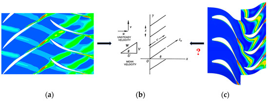
Figure 1.
Fan-linearized acoustic modeling and actual flow processes in low-pressure turbines. (a) Fan wake interaction process; (b) Linear thin flat-plate assumption [37]; (c) Turbine wake interaction process.
2.2. Two-Flat-Plates Assumption
For subsonic flow, the dominant source term is the dipolar integral that only depends on unsteady loading on hard walls. As a result, the most developed analytical methods mainly focus on a dipolar source, and turbine noise is no exception. It is often necessary to establish some assumption about blade geometry and flow condition. The blade is often split into segments (Strip Theory) and each segment is assumed to be a very thin flat plate with a local mean stagger angle and zero attacking angle (thin-flat-plate assumption). Based on above hypotheses, it is noted that the thin-flat-plate assumption of a fan blade is applicable, but the rationality of using it on a turbine blade is untraceable, let alone the prediction of turbine broadband noise using those broadband noise models [19,20].
To solve such a problem, two-flat-plates assumption for high cambered turbine blade is initially proposed here as seen in Figure 2. () and () are the axial chord length and the stagger angle for section ‘I’ (‘II’), respectively. LP (TP) represents the leading edge (the trailing edge) point and JP is the junction point of the entire segment and is also the connection point between the section ‘I’ and the section ‘II’. In such assumption, that how to couple the two sections with different parameters like stagger angles and chordal coordinates carry paramount importance.
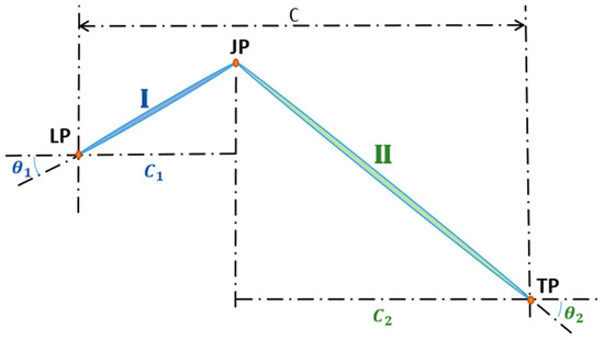
Figure 2.
Two-flat-plate assumption for turbine blade.
2.3. Turbine Broadband Noise Model
Based on the above two-flat-plate assumption, a turbine broadband noise model would be established here. Starting with the basic acoustic equation, for the sound field in a circular or an annular hard-walled duct, the sound pressure consists of a linear superposition of different duct acoustic modes [28]:
in which,
Under the coordinate system established by the original thin-flat-plate assumption, as shown in Figure 3a, can be expressed as follows:
in which,
where is the observation point outside the source region in a cylindrical coordinate system and is the source point. represents, respectively, a downstream/upstream direction, only considering the former for turbine noise here. represents an eigenfunction solved by two types of Bezier functions and is an eigenvalue. is the unsteady loading at source point and represents the outer normal vector of the source point. is the axial wave number. , , and , respectively, represent the inflow Mach number, sound speed, angular frequency and source areas. can be expressed as follows:
where and are, respectively, the outer and inner duct radii.
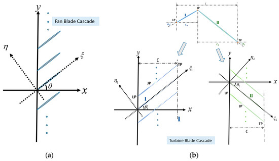
Figure 3.
Coordinate systems with different assumptions: (a) Coordinate system with one-flat-plate assumption (fan blade cascade); (b) Coordinate system with two-flat-plate assumption (turbine blade cascade).
When the blade is regarded as a flat plate and the annular cascade is unwrapped to a linear cascade, as assumed in LINSUB, the physical meaning of is the pressure difference between the pressure surfacer and the suction surface, which can be expressed as . and are the sound pressure of the pressure surface and the suction surface and V is the blade number. is the unsteady lift solved by LINSUB. Additionally, the normal vector is , as shown in Figure 3a.
At present, when solving Equation (3), two terms are crucial. The first one is the ‘load’ term , which is solved by LINSUB [33] and can be transformed into Equation (6):
After using the Fourier transform for , the ‘load’ term is written as follows:
The other one ‘geometry’ term can be expressed as follows:
After Fourier transform for , the can be written, briefly, as follows:
where is the upwash velocity on the blade surface and is obtained from LINSUB.
The above process is based on the thin-flat-plate assumption. At present, the set-up of the coordinate system is shown in Figure 3b. In such a coordinate system, the original section ‘I’ is artificially extended backward until the axial chord length changed to . Likewise, the original section ‘II’ is extended forward. Then, coupling the two sections, Equation (9) can be written as follows:
in which,
where NP is defined as the ratio of the axial chord length of section ‘I’ to the total axial chord length . It is essential to be noted that, although the two sections have been extended backward or forward in the coordinate system, as shown in Figure 3, the chordwise integration is from 0 to NP for the first section ‘I’ and the corresponding range is from NP to 1 for the section ‘II’.
Now, the sound power in the infinite hard wall is expressed as follows:
in which,
where represents the statical averaging within the integral sign.
Then, Equation (13) leads to the following:
and by applying the Liepmann spectrum, we obtain the following:
in which,
where TKE is the turbulent kinetic energy and is the turbulence dissipation rate. Both can be extracted from the RANS result, which is the reason that such a model is called the RANS-informed analytical method. The place to extract the turbulent information used for section I is broadly stated as before the leading edge of the downstream blade. And the turbulent information as input for section II is assumed to be the same as that of section I.
Then, let be the following:
Substituting Equation (14) into Equation (13), the cross-power spectral density becomes
Then, substituting Equations (15)~(17) and Equation (20) into Equation (12) can result in the final expression of the sound power spectrum function. This formula is suitable for the broadband noise prediction of a turbine with high blending angle.
3. Validation of RI-TP Model
Firstly, a single-stage axial cold turbine acoustic test rig (NPU-Turb) at the Turbomachinery Aerodynamic and Acoustic Laboratory (TAAL) of Northwestern Polytechnical University (NPU) was used for validation and study. The experimental setting and validation results are described in detail below. Then, the DDES/AA hybrid model was also applied to further validate the RI-TP model.
3.1. Experimental Validation
3.1.1. Turbine Acoustic Test Rig NPU-Turb
The sketch of the NPU-Turb is depicted in Figure 4. After the downstream of the turbine blade row, there is a rotating measurement duct for mounting a microphone array to collect sound pressure data at different circumferential and axial locations, after which, there are two-turn fixed microphone arrays whose signals can be used directly for mode-decomposition at low-frequencies. Additionally, in order to reduce the influence of external ‘dirty’ sources on microphone signals, only the measurement duct is installed in the semi-anechoic chamber and the remaining parts are located outside. The basic design parameters of the NPU-Turb are shown in Table 1.
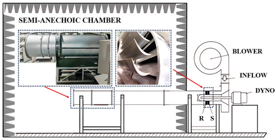
Figure 4.
Sketch of the NPU-Turb acoustic test rig.

Table 1.
Design parameters of the NPU-Turb.
3.1.2. Experimental Setting
Figure 5 gives the maximum cut-on modal orders below 10 KHz of the NPU-Turb at the designed rotation speed. The maximum values of the circumferential modal order m and radial modal order n are, respectively, 44 and 14. In order to achieve the accurate identification of the duct acoustic modes for experimental measurement, sound pressure signals need to be collected at more than 88 circumferential locations at one fixed axial location and the number of turns of the circumferential microphone array distributed along the axial direction should be at least 28 without separating incident and reflected waves. As a result, two equally spaced linear axial arrays 180° apart, each including thirty microphones, are applied in this experiment and sound pressure data are collected every 4°, as is shown in Figure 6. In addition, there are four fixed microphones behind the rotating measurement duct for mode-decomposition using the reference microphone method.
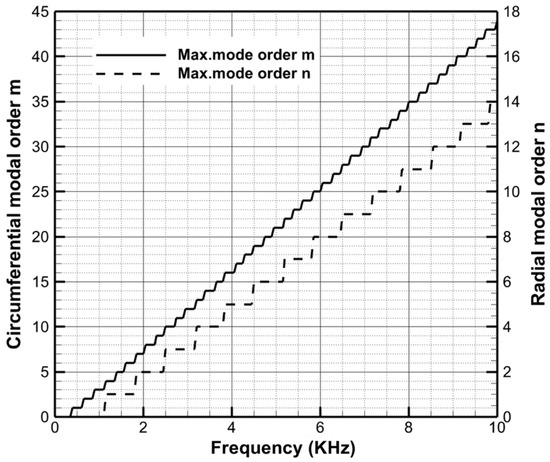
Figure 5.
Maximum cut-on modal orders of NPU-Turb.
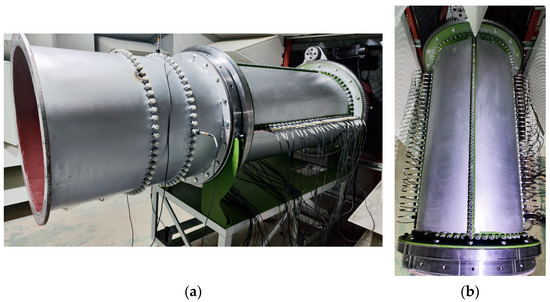
Figure 6.
Microphone array setting of duct acoustic modes experiment: (a) Horizonal view; (b) Overhead view.
The reference microphone mode-decomposition method is premised on the assumption that the different acoustic modes are completely uncorrelated with each other and this can greatly simplify the mode-decomposition process, in which the correlation terms between different circumferential modes are equal to zero. Thus, the sound field correlation should be analyzed first.
In order to eliminate the effect of local turbulent pressure fluctuation on the microphone signals, Michalke [41] used the cross-correlation function of the microphone sound pressure signals at three different spatial locations for evaluating the sound field correlation in the duct:
where , and , respectively, denote the correlation functions of the microphone signals at three different positions, , , and , respectively, denote the phases of the corresponding correlation functions. is real if the duct acoustic modes are perfectly correlated with each other, in which case, the phase is equal to zero. Otherwise, it is complex.
3.1.3. RANS Simulation of RI-TP Model
The developed RI-TP model requires running RANS to provide the input parameters. The main inputs are the circumferential-averaged radial-distributed turbulent kinetic energy and the turbulent dissipation rate at the leading edge of downstream blade. As Figure 7 shows, the computational domain contains four parts: inlet region with three-times stator axial chord length, stator region, rotor region and outlet region with four-times rotor axial chord length. The plane named ‘EXTRACTION’ located at the rotor leading edge is used to extract the turbulent information. Then, the effect of the axial location of ‘EXTRACTION’ on the model prediction results will be discussed below.
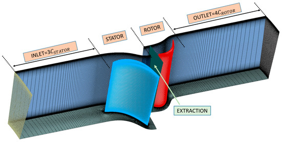
Figure 7.
Computational domain of NPU-Turb for RANS.
O-type grids are used around blades and H-type grids are used for other regions. The total pressure and the total temperature are used as stator inlet boundary conditions and the static pressure is set for a rotor outlet boundary condition. The shear stress transport (SST) turbulence model with a Gamma–Theta transitional model is used. A high resolution scheme is used for both the advection and the transient scheme.
The changes in circumferential mass-averaged TKE and TLS (turbulent integration length scale) with a nodes number have been given in Figure 8. It indicates that turbulent information can be considered unchanged when the nodes number is larger than 7 million for the computational region shown in Figure 7. As a result, the case of 7 million nodes is used.
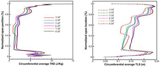
Figure 8.
Changes in circumferential average TKE and TLS with nodes number (EXTRACTION = C as shows in 14th figure of this paper): (left): Circumferential average TKE; (right): Circumferential average TLS.
3.1.4. Basic Input Parameters of NPU-Turb for RI-TP Model
Except for the turbulent information from the RANS result being used as an input, there are some geometric parameters. As mentioned above, , , NP, etc., at different span radii have been given in the RI-TP model. Table 2 gives the corresponding mean values at different span radii of the NPU-Turb. Those values are derived from the NPU-Turb design results and is shown in absolute value.

Table 2.
Some input parameters of the NPU-Turb.
3.1.5. Experimental Validation Results
As described in Section 3.1.2, the sound field correlation should be discussed before using the reference microphone method. Using Michalke’s method, the microphone signals of the three positions 1/30/45 and 15/31/60 are used as an example (the microphone order is shown in Figure 9a and the phase distribution of the cross-correlation function is shown in Figure 9b,c). It can be seen that the phase angle changes drastically below 10 KHz, which means the turbine wake interaction broadband noise is essentially uncorrelated and the reference microphone decomposition method can be used here.
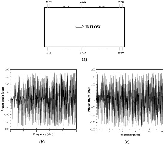
Figure 9.
Phase information of different microphones: (a) Microphone order; (b) 1/30/45; (c) 15/31/60.
Figure 10 compares the PWL (sound power level) between the RI-TP model prediction results and experimental results at the designed and the off-designed rotation speed. Below about 2 KHz, the difference between the modal and experiment data are mainly due to the dynamometer’s shaft which directly connects to the rotor shaft. A slight misalignment between the two shafts themselves and the junction of the two shafts can lead to background noise. Moreover, such background noise is proportional to the operating power. Unfortunately, since the test rig cannot lock the rotational speed, the effects of this background noise cannot be removed. As a result, the frequency range between 2 KHz and 10 KHz is effective.
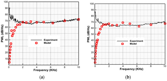
Figure 10.
Validation result of RI-TP model with experiment data (removing tonal noise): (a) Designed rotation speed; (b) Off-designed rotation speed (90% designed speed).
3.2. Numerical Validation
3.2.1. Brief Discussion of CFD/AA Hybrid Model
Aerodynamic noise is the pressure fluctuation in the flow field region, and its governing equation is consistent with the Navier–Stokes equation. But the difference between the acoustic variables and the flow field variables generating the sound in terms of energy and scale is very large, coupled with the fact that acoustic propagation tends to have a very large spatial scale, which means that obtaining the acoustic field through the full-field solving of the NS equation is a very demanding task both for the computer hardware and for the numerical simulation method.
In order to solve the conflict between computational accuracy and resource limitation, the CFD/AA hybrid method has been used since 1952 [42,43]. For different noise sources, different scales of CFD need to be run. Two steps can be divided briefly. First, the unsteady loading on the blade surface is extracted from the CFD results. Second, the unsteady loading is used as a noise source into an AA (Acoustic Analogy) equation to solve the noise propagation.
For periodic wake interaction tonal noise, URANS (Unsteady Reynold Averaged Navier–Strokes equation) is enough, while for the wake turbulence interaction broadband noise of turbomachinery, in order to capture enough source information, the LES (Large Eddy Simulation) method is usually applied. But the demand for a grid within the boundary layers is still overwhelming and this is why the DES-class method surges ahead.
The AA equation also has different forms. In a free field, the most commonly used acoustic analogy is the Ffowcs Williams and Hawkings’s analogy (FWH) that deals with solid bodies in motion in a quiet and uniform reference medium [44]. Such a theory was soon applied to rotating machinery [45]. Based on the FWH equation, Goldstein [29] proposed an extension of the FWH analogy by replacing the free-field Green’s function with the Green’s function in an infinite cylinder in the presence of an axial uniform flow [29].
3.2.2. Introduction of DES-Class Method
The DES method was originally proposed to improve the predictive power of turbulence models in large separation regions and reduce unnecessary mesh requirements within the boundary layer [46,47].
The ideal behind the DES model switches from the RANS model to the LES model in regions where the local mesh spacing is smaller than the turbulent length as predicted by the RANS model. The ‘switch’ function can be written as follows:
in which . When the computational domain switches between RANS and LES, the numerical solution method also switches between an upwind scheme and a center-differential scheme. When the switch function is controlled only by the grid spacing, it tends to lead to the “grid-induced” separation problem, and in order to solve this problem, the DDES method introduces the function , which delays the conversion process from RANS to LES, in the original control function:
can be expressed using different forms. Mentor [48] uses a hybrid function employed by the SST model. Inspired by Mentor [48], Spalart [49] extended it further by extending the function so that it is not only applicable to SST models, but the following switch function can be used whenever a RANS model involves eddy viscosity:
in which,
where is the kinematic vortex viscosity, is the molecular viscosity, is the velocity gradient, is the von Karmen coefficient and is the distance of the grid from the wall. is the LES calculation region. In 2012, Gritskevich [50] further developed it as
in which, . can be written as follows:
where is the strain rate and the degree of rotation. It follows that the core of the development of the DES-class method is the establishment of different switch functions.
For the turbine wake interaction broadband noise, wake information is the most significant factor and the DDES has the ability to accurately capture the noise source information. And DES-class methods are now commonly used in ANSYS (Version 2022), aiding in computational studies of NPU-Turb.
3.2.3. Computational Mesh and Setting
Figure 11a shows the computational domain, in which the extended region is to make the smooth transition from fine mesh around the blade to course mesh at the outlet. A structured grid is applied in all domains and the total nodes numbers is about 27.65 million. Figure 11b,c respectively, gives the local mesh around the blades at the meridian plane and on both blade surfaces. Figure 12 gives the distribution on the rotor surfaces, which indicates that the mesh in the normal blade surface is enough to capture noise source information. And the of the switch function is shown in Figure 13. The blue region is the LES region.
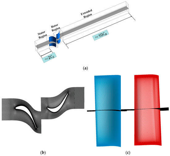
Figure 11.
Computational domain and local mesh of NPU-Turb for DDES: (a) Computational region; (b) Mesh in meridian plane; (c) Mesh on blade surface.
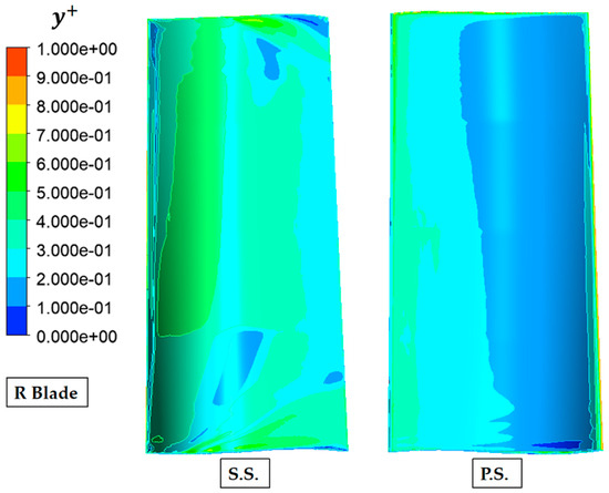
Figure 12.
distribution on rotor surfaces. (Left): S.S.: Suction Surface; (Right): P.S.: Pressure Surface. (there is no negative value).
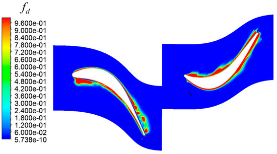
Figure 13.
distribution of switch function at 50% spanwise section. (There is no negative value).
In the current simulation, the blade surfaces are set as no-slip walls and the periodic boundary is used in the circumferential direction. An SST (shear stress transport) turbulence model is used for the steady simulation and the DDES model is used for the unsteady simulation. For the unsteady case, a central difference for the advection scheme and the second order backward Euler for the transient scheme are applied. For the unsteady calculation, the time step is 0.00001 s with 50 steps needed for one blade passage. In order to make the computation reach the statistical steady state as soon as possible, the DDES is initiated with the pre-converged RANS results as the initial field, and 4000 timesteps (through 80 blade passages corresponding two whole cycles) are run first to obtain the statistical steady state, and then another 4000 timesteps are run forward and outputted every two steps for extracting the time series of the blade surface pressure information.
3.2.4. Acoustic Calculation Method of CFD/AA Hybrid Model
The Goldstein analogy equation [28] replaced the free-field Green’s function with the Green’s function in an infinite cylinder or an annular duct with an axial uniform flow and is suitable for duct noise calculation. Only considering the dipole sources, the PWL of broadband noise can be statistically averaged as follows:
where is consistent with Equation (2) and the only difference is that the unsteady loads coming from numerical calculations.
3.2.5. Hybrid Model’s Validation Result
Figure 14 compares the PWL of the turbine wake interaction noise among the RI-TP model prediction results, the experimental data and the DDES/AA hybrid model prediction results at the designed rotation speed. On the one hand, the consistency of the three methods in spectrum prediction in the 2 KHz~10 KHz range further validates the accuracy of the RI-TP model. On the other hand, that there is little difference between the RI-TP model and the DDES/AA hybrid model below 2 KHz proves the experimental data have serious ‘dirty’ noise at such a frequency range and the difference below 2 KHz in Figure 10 is not worthy of attention. As a whole, the accuracy of the RI-TP model for the turbine wake interaction broadband noise developed in this paper is sufficient to accurately predict the broadband noise spectral distribution.
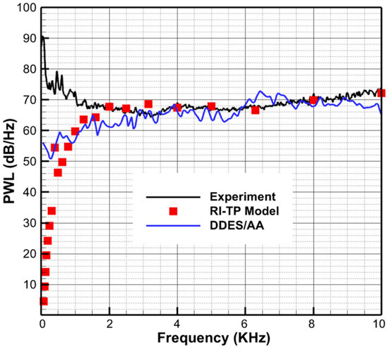
Figure 14.
Validation result of the RI-TP model with experiment data and DDES/AA hybrid model (removing tonal noise, designed rotation speed).
4. Studies of the RI-TP Model
In order to quantify the benefits of the two-flat-plates (TP) assumption, the prediction result of a one-flat-plate assumption, extended in section I and in section II for turbine blade on turbine noise, have been compared here. Furthermore, this section, respectively, discusses the influence of different factors like the location of the Junction Point (JP), the location for extracting turbulence from the RANS result, and end walls.
4.1. Flat-Plate Assumption
To aptly illustrate the gain in prediction accuracy from the two-flat-plate (TP) assumption, the prediction result under the old linear flat-plate assumption for turbine blade is shown in Figure 15, with the coordinate system also given in Figure 15a below. In addition, the contribution of the single extended section (I′ or II′) compared with the present ‘I + II’ has also been compared here. Figure 15b gives the prediction results in the four kinds of assumptions. It can easily be found that the present TP assumption can greatly increase PWL at most frequencies. For real turbine aero-acoustic design, there is a clear upper limit indicator for noise level. Only if the turbine noise prediction is sufficiently accurate will it be possible to know if the various acoustic mitigation strategies meet the overall requirements.
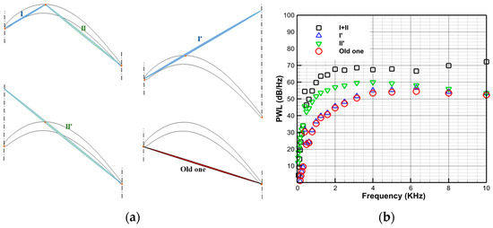
Figure 15.
The effect of flat-plate assumption: (a) Four kinds of assumptions for simplified turbine blade; (b) Comparation with different assumptions of turbine blade (NP = 0.4, EXTRACTION = C, designed rotation speed).
4.2. JP Location
The value of NP, defined as the ratio of axial chord length of section ‘I’ to the total axial chord length , is critical in the RI-TP model, which can be seen from Equation (11). Figure 16 gives the predicted results with NP changes from 0.20 to 0.80. It can be seen that the larger the NP value, the smaller the PWL at almost all frequencies, but the trend tends to be moderate, especially at high frequencies larger than 5 KHz. Such a phenomenon can be explained by the Kernel function of the LINSUB and the changes of contribution between section I and II. When NP is small (NP = 0.2), the whole load distribution consists of little of section I and most of section II, which causes an unreal spectral distribution. Such a phenomenon does not occur for NPs > 0.4 because section I has been dominant. The effect of changes and rotor turning angle changes act as a counteract for each other. And this also indicates that section II mainly has the effect of gaining the PWL of the spectrum but the trend of spectrum distribution is dominated by section I.
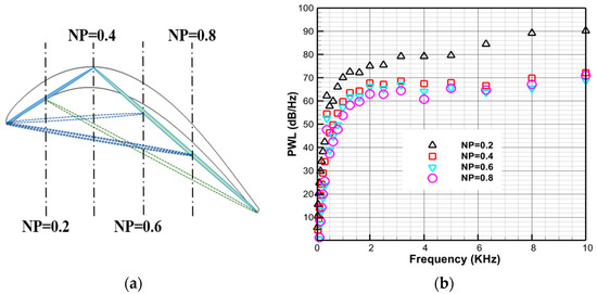
Figure 16.
The effect of NP value: (a) NP definition; (b) Comparation with different NP values (EXTRACTION = C, designed rotation speed).
4.3. Extraction Location for Turbulent Information
The turbulent kinetic energy and the turbulence dissipation rate in the RANS-informed model are key input parameters. The extraction location is only required at the blade leading edge but not as a clear quantitative limitation. Here, we have studied the effect of three equally spaced surfaces for the turbulent information of section I on the model prediction results. In Figure 17a, A, B and C represent the extraction surfaces located at 50%, 70% and 90% of the axial stator–rotor spacing, respectively. Figure 17b shows the results, which indicate that slight differences in turbulence information at three surfaces before the leading edge do not have a significant effect on the PWL of the RI-TP prediction result. As a result, the EXTRACTIO=C is used for all other cases.
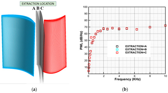
Figure 17.
The effect of extraction location for turbulent information on model prediction result (NP = 0.4, designed rotation speed): (a) Description of extraction location for turbulent information; (b) Comparation with different flat-plate assumptions.
5. Discussion
The need for a lower number of turbine blades and highly loaded turbine rows in future UHBR engines would cause serious noise problems and the current lack of turbine noise research urgently requires the development of noise prediction modeling and noise control methods. It is in this context that the research in this paper is carried out.
A rapid model, named the RI-TP model, for predicting turbine wake interaction broadband noise is developed in this paper and its accuracy is validated by both the acoustic experimental data of the single axial test rig NPU-Turb and the prediction results of a DDES/AA hybrid method. The most significant contribution of the RI-TP model lies in the formulation of the two-flat-plate assumption which can effectively take into account noise variations due to the geometrical characteristics of the large turning angle of the turbine blade. A comparison of the prediction results following the two-flat-plate assumption and the different one flat-plate assumption has shown that the former can effectively improve the prediction accuracy below 10 KHz. Finally, more experimental data are needed to test the RI-TP model’s applicability and limitations and such works can be further performed in the future if possible. Due to the benefits of its rapid prediction ability and aerodynamic design process, coupled with the high aerodynamic performance of the integrated design of the low-noise radiation turbine stage, the RI-TP model would make the possibility of generating “turbine noise storms” less likely or even disappear.
In addition, the development of a turbine noise prediction model requires a consideration of the impact of two other factors including rotor blade thickness and multistage effect. First, the applicability of a very thin flat-plate assumption on a turbine blade is doubtful and its impact is currently difficult to assess quantitatively. Second, the multistage design of engine turbine would yield a complex noise generation and propagation problem, especially in a UHBR engine with much less stage-filtering efficiency.
6. Conclusions
An analytical method named the RI-TP model with a novel two-flat-plates assumption, corresponding to the large turning angle of the turbine blade, has been developed to predict turbine wake turbulence broadband noise. Taking the single axial turbine rig NPU-Turb as the object, its accuracy has been double validated using experimental data and numerical data with a CFD/AA hybrid model. In the future, the effect of blade thickness and multistage design on turbine noise should be further studied, which would significantly increase its academic value and engineering applications.
Author Contributions
Conceptualization, K.X. and W.Q.; methodology, K.X. and W.C.; software, K.X.; validation, K.X., W.C. and S.A.; formal analysis, K.X.; data curation, K.X.; writing—original draft preparation, K.X.; writing—review and editing, W.C., S.A. and W.Q.; visualization, K.X.; supervision, W.Q.; funding acquisition, W.Q.; All authors have read and agreed to the published version of the manuscript.
Funding
This study was co-supported by the National Science and Technology Major Project of China (No. 2017-II-0008-0022), Aero Engine and Gas Turbine Basic Science Center (P2022-A-II-003-001, P2022-B-II-011-001) and the National Natural Science Foundation of China (Nos. 52276038, 51936010, 52106056).
Data Availability Statement
The raw data supporting the conclusions of this article will be made available by the authors on request.
Conflicts of Interest
The authors declare no conflicts of interest.
References
- Moreau, S. Turbomachinery Noise Predictions: Present and Future. Acoustics 2019, 1, 92–116. [Google Scholar] [CrossRef]
- Rolf, R.; Richard, S. Fundamentals of High Lift for Future Civil Aircraft, 1st ed.; Springer Nature Switzerland AG: Cham, Switzerland, 2021; pp. 579–592. [Google Scholar]
- Hughes, C. NASA Collaborative Research on the Ultra High Bypass Engine Cycle and Potential Benefits for Noise, Performance, and Emissions; Technical Memorandum TM-2013-216345; NASA: Washington, DC, USA, 2013. [Google Scholar]
- Hultgren, L.S. Editorial: Emerging importance of turbine noise. Int. J. Aeroacoust. 2011, 10, i–iv. [Google Scholar] [CrossRef]
- Nesbitt, E. Towards a quieter low pressure turbine: Design characteristics and prediction needs. Int. J. Aeroacoust. 2011, 10, 1–15. [Google Scholar] [CrossRef]
- Xiang, K.S.; Chen, W.J.; Wang, L.F.; Tao, M.Y.; Qiao, W.Y. Turbine tonal noise prediction using an improved quasi-3D linear model. Aerosp. Sci. Technol. 2022, 123, 107437. [Google Scholar] [CrossRef]
- Ventres, C.S.; Theobald, M.A.; Mark, W.D. Turbofan Noise Generation, Volume 1: Analysis; NASA: Washington, DC, USA, 1987. [Google Scholar]
- Nallasamy, M.; Envia, E. Computation of rotor wake turbulence noise. J. Sound Vib 2005, 282, 649–678. [Google Scholar] [CrossRef]
- Posson, H.; Roger, M.; Moreau, S. On a uniformly valid analytical rectilinear cascade response function. J. Fluid Mech. 2010, 663, 22–52. [Google Scholar] [CrossRef]
- Posson, H.; Moreau, S.; Roger, M. On the use of a uniformly valid analytical cascade response function for fan broadband noise predictions. J. Sound Vib. 2010, 329, 3721–3743. [Google Scholar] [CrossRef]
- Posson, H.; Moreau, S.; Roger, M. Broadband noise prediction of fan outlet guide vane using a cascade response function. J. Sound Vib. 2011, 330, 6153–6183. [Google Scholar] [CrossRef]
- Masson, V.; Posson, H.; Sanjosé, M.; Moreau, S.; Roger, M. Fan-OGV interaction broadband noise prediction in a rigid annular duct with swirling and sheared mean flow. In Proceedings of the 22nd AIAA/CEAS Aeroacoustics Conference (AIAA 2016-2944), Lyon, France, 30 May–1 June 2016. [Google Scholar]
- Rai, M.; Madavan, N. Multi-Airfoil Navier–Stokes Simulations of Turbine Rotor-Stator Interaction. J. Turbomach. 1990, 112, 377–384. [Google Scholar] [CrossRef]
- Gerolymos, G.; Michon, G.; Neubauer, J. Analysis and application of chronic periodicity in turbomachinery rotor/stator interaction computations. J. Propuls. Power 2002, 18, 1139–1152. [Google Scholar] [CrossRef]
- Giles, M.B. Calculation of unsteady wake/rotor interaction. J. Propuls. Power 1988, 4, 356–362. [Google Scholar] [CrossRef]
- Guédeney, T.; Gomar, A.; Gallard, F.; Sicot, F.; Dufour, G.; Puigt, G. Non-uniform time sampling for multiple-frequency harmonic balance computations. J. Comput. Phys. 2013, 236, 317–345. [Google Scholar] [CrossRef]
- Chen, S.; Dooler, G.D. Lattice Boltzmann method for fluid flows. Ann. Rev. Fluid Mech. 1998, 30, 329–364. [Google Scholar] [CrossRef]
- Brès, G.; Pérot, F.; Freed, D. Properties of the Lattice–Boltzmann Method for Acoustics. In Proceedings of the 15th AIAA/CEAS Aeroacoustics Conference (AIAA 2009-3395), Miami, FL, USA, 11–13 May 2019. [Google Scholar]
- Ju, H.; Mani, R.; Vysohlid, M.; Sharma, A. Investigation of fan-wake/ outlet-guide-vane interaction broadband noise. AIAA J. 2015, 53, 3534–3550. [Google Scholar] [CrossRef]
- Ju, H.B. Effects of vane sweep on fan-wake/outlet-guide-vane interaction broadband noise. In Proceedings of the 22nd AIAA/CEAS Aeroacoustics Conference, Lyon, France, 30 May–1 June 2016; AIAA: Reston, VA, USA, 2016. [Google Scholar]
- Guérin, S.; Kissner, C.; Kajasa, B.; Jaron, R.; Behn, M.; Pardowitz, B.; Tapken, U.; Hakansson, S.; Meyer, R.; Enghardt, L. Noise prediction of the ACAT1 fan with a RANS-informed analytical method: Success and challenge. In Proceedings of the 25th AIAA/CEAS Aeroacoustics Conference, Delft, The Netherlands, 20–23 May 2019. [Google Scholar]
- Lewis, D.; Moreau, S.; Jacob, M. On the Use of RANS-informed Analytical Models to Perform Broadband Rotor-Stator Interaction Noise Predictions. In Proceedings of the 25th AIAA/CEAS Aeroacoustics Conference, Delft, The Netherlands, 20–23 May 2019. [Google Scholar]
- Tong, H.; Ll, L.; Wang, L.; Mao, L.; Qiao, W. Investigation of rotor–stator interaction broadband noise using a RANS-informed analytical method. Chin. J. Aeronaut. 2021, 34, 53–66. [Google Scholar] [CrossRef]
- Karman, T. Progress in the statistical theory of turbulence. Proc. Natl. Acad. Sci. USA 1948, 34, 530–539. [Google Scholar] [CrossRef]
- Liepmann, H.W. Extension of the statistical approach to buffeting and gust response of wings of finite span. J. Aeronaut. Sci. 1955, 22, 197–200. [Google Scholar] [CrossRef]
- Liepmann, H.W.; Laufer, J.; Liepmann, K. On the Spectrum of Isotropic Turbulence; NASA: Washington, DC, USA, 1951. [Google Scholar]
- Grace, S.; Wixom, A.; Winkler, J.; Sondak, D.; Logue, M.M. Fan Broadband Interaction Noise Modeling. In Proceedings of the 18th AIAA/CEAS Aeroacoustics Conference (33rd AIAA Aeroacoustics Conference), Colorado Springs, CO, USA, 4–6 June 2012. [Google Scholar]
- Laborderie, L.; Moreau, S.; Berry, A. Compressor Stage Broadband Noise Prediction Using a Large-Eddy Simulation and Comparisons with a Cascade Response Model. In Proceedings of the 19th AIAA/CEAS Aeroacoustics Conference, Berlin, Germany, 27–29 May 2013. [Google Scholar]
- Goldstein, M.E. Aeroacoustics, 1st ed.; McGraw-Hill International Book Company: New York, NY, USA, 1976. [Google Scholar]
- Mani, R. Noise due to interaction of inlet turbulence with isolated stators and rotors. J. Sound Vib. 1971, 17, 251–260. [Google Scholar] [CrossRef]
- Amiet, R.K. Acoustic radiation from an airfoil in a turbulent stream. J. Sound Vib. 1975, 41, 407–420. [Google Scholar] [CrossRef]
- Glegg, S.A.L. The response of swept blade row to a three-dimensional gust. J. Sound Vib. 1999, 227, 29–64. [Google Scholar] [CrossRef]
- Smith, S.N. Discrete Frequency Sound Generation in Axial Flow Turbomachines; HM Stationery Office: London, UK, 1972. [Google Scholar]
- Whitehead, D.S. Vibration and Sound Generation in a Cascade of Flat Plates in Subsonic Flow; HM Stationery Office: London, UK, 1972. [Google Scholar]
- Kaji, S.; Okazaki, T. Generation of sound by rotor-stator interaction. J. Sound Vib. 1970, 13, 281–307. [Google Scholar] [CrossRef]
- Kaji, S. Noncompact source effect on the prediction of tone noise from a fan rotor. In Proceedings of the 2nd Aeroacoustics Conference, Hampton, VA, USA, 24–26 March 1975. [Google Scholar]
- Hanson, D.B. Coupled 2-Dimensional Cascade Theory for Noise and Unsteady Aerodynamics of Blade Row Interaction in Turbofans. Volume 1: Theory Development and Parametric Studies; NASA: Washington, DC, USA, 1995. [Google Scholar]
- Hanson, D.B. Coupled 2-Dimensional Cascade Theory for Noise and Unsteady Aerodynamics of Blade Row Interaction in Turbofans. Volume 2: Documentation for Computer Code CUP2D; NASA: Washington, DC, USA, 1995. [Google Scholar]
- Cheong, C.; Joseph, P.; Soogab, L.E.E. High frequency formulation for the acoustic power spectrum due to cascade-turbulence interaction. J. Acoust. Soc. 2006, 119, 108–122. [Google Scholar] [CrossRef]
- Pedro, C.L.; Adolfo, S. A Frequency Domain Model for Turbine Interaction Broadband Noise: Comparison with Measurements. In Proceedings of the AIAA/CEAS Aeroacoustics Conference, Atlanta, GA, USA, 25–29 June 2018. [Google Scholar]
- Michalke, A.; Arnold, F.; Holste, F. On the Coherence of the Sound Field in a Circular Duct with Uniform Mean Flow. J. Sound Vib. 1996, 190, 261–271. [Google Scholar] [CrossRef]
- Lighthill, M.J. On sound generated aerodynamically, I. General theory. Proc. Roy. Soc. Lond. Ser. A Math. Phys. Sci. 1952, 211, 564–587. [Google Scholar]
- Lighthill, M.J. On sound generated aerodynamically, II. Turbulence as a source of sound. Proc. Roy. Soc. Lond. Ser. A Math. Phys. Sci. 1954, 222, 1–32. [Google Scholar]
- Ffowcs Williams, J.E.; Hawkings, D.L. Sound Generation by Turbulence and Surfaces in Arbitrary Motion. Philo. Trans. R. Soc. Lond. A Math. Phys. Sci. 1969, 264, 321–342. [Google Scholar]
- Ffowcs-Williams, J.E.; Hawkings, D.L. Theory relating to the noise of rotating machinery. J. Sound Vib. 1969, 10, 10–21. [Google Scholar] [CrossRef]
- Spalart, P.R.; Jou, W.H.; Strelets, M.; Allmaras, S.R. Comments on the feasibility of LES for wings, and on a hybrid RANS-LES approach. In Advances in DNS/LES; Liu, C., Liu, Z., Eds.; ResearchGate: Berlin, Germany, 1997; pp. 137–147. [Google Scholar]
- Shur, M.; Spalart, P.R.; Strelets, M.; Travin, A. Detached-eddy simulation of an airfoil at high angle of attack. In Engineering Turbulence Modelling and Experiments; Elsevier Science Ltd.: Amsterdam, The Netherlands, 1999. [Google Scholar]
- Menter, F.R.; Kuntz, M. Adaptation of eddy-viscosity turbulence models to unsteady separated flow behind vehicles. In The Aerodynamics of Heavy Vehicles: Trucks, Buses, and Trains; Springer: Berlin, Germany, 2004; pp. 339–352. [Google Scholar]
- Spalart, P.R.; Deck, S.; Shur, M.L.; Squires, K.D.; Strelets, M.K.; Travin, A. A new version of detached-eddy simulation, resistant to ambiguous grid densities. Theor. Comput. Fluid Dyn. 2006, 20, 181–195. [Google Scholar] [CrossRef]
- Gritskevich, M.S.; Garbaruk, A.V.; Schütze, J.; Menter, F.R. Development of DDES and IDDES Formulations for the k-ω Shear Stress Transport Model. J. Flow Turbul. Combust. 2012, 88, 431–449. [Google Scholar] [CrossRef]
Disclaimer/Publisher’s Note: The statements, opinions and data contained in all publications are solely those of the individual author(s) and contributor(s) and not of MDPI and/or the editor(s). MDPI and/or the editor(s) disclaim responsibility for any injury to people or property resulting from any ideas, methods, instructions or products referred to in the content. |
© 2024 by the authors. Licensee MDPI, Basel, Switzerland. This article is an open access article distributed under the terms and conditions of the Creative Commons Attribution (CC BY) license (https://creativecommons.org/licenses/by/4.0/).