Article

Research on Intelligent Design of Geometric Factor Encoding for Aircraft Engine Turbine Structures

School of Aircraft Engineering, Nanchang Hangkong University, Nanchang 330063, China
*
Author to whom correspondence should be addressed.
Aerospace 2024, 11(3), 186; https://doi.org/10.3390/aerospace11030186
Submission received: 23 January 2024 / Revised: 19 February 2024 / Accepted: 23 February 2024 / Published: 26 February 2024
(This article belongs to the Section Aeronautics)

Abstract

:
In recent years, with the rapid development of computer technology and artificial intelligence design technology, multiple possible design solutions can be quickly generated by transforming the experience and knowledge of structural design into computer executable rules and algorithms. To achieve intelligent design of aircraft engines, this paper proposes an encoding model for the turbine rotor structure of aircraft engines using geometric encoding technology. The turbine rotor structure of aircraft engines is divided into several units according to geometric similarity types, these units continue to be divided into attribute sets according to their functional types, connection relationships, and material properties. These attribute sets can be encoded using geometric encoding technology. The experiment simulated that these codes, for the point cloud modeling of turbine rotor structure, can be quickly achieved and they combine various algorithms to display the point cloud model of the turbine rotor in the Microsoft Visual studio MFC class library. The results show that by creating geometric codes for the turbine rotor of aircraft engines, it is possible to quickly create and display point cloud models of the turbine rotor structure, laying the foundation for subsequent application of machine learning to solve and find the optimal design solution.

1. Introduction

With the rapid development of computer technology, traditional product design can no longer meet the personalized design of technology as the object of specific customers or customer groups. The inconsistency between the newly adopted advanced production manufacturing process and traditional design methods is a bottleneck in design. Therefore, in manufacturing production, design becomes the largest direct or indirect cost area, and researching intelligent design of digital products has become an urgent problem to be solved [1,2,3,4]. The same is true in the aerospace field.
Aircraft engines are a key product in the development of the aviation industry, and the quality of engines directly determines the performance of aircraft. Moreover, the progress of engine development is also a decisive factor in the overall progress of aircraft development [5,6]. In the field of aviation engine turbocharging, the turbine operates at high temperatures and speeds, and the working conditions are extremely demanding, requiring a long lifespan and high reliability, while the quality is strictly controlled. Therefore, structural design is very difficult. In the structural design stage, static strength, stiffness, vibration, and rotor dynamics analysis should be conducted on the blades, discs, and shafts to determine the main dimensions of the structure. With a preliminary structural concept diagram, strength calculations need to be carried out to compare the stress levels, stress distribution, and stiffness of different structures, to select and optimize structural design. In this design process, it is always necessary to integrate, analyze, and compromise with other factors. The design process is often repetitive, and the corresponding strength calculation also needs to be repeated [7,8]; this makes the design phase time-consuming. One of the main problems of the aircraft engine is the high costs at all stages of the design and production. Reducing costs and improving competitiveness essentially begin with the accurate and efficient estimate of the resource for the manufacture of the products, including labor and material costs [9,10,11,12].
Intelligent design, as an important aspect of the field of artificial intelligence, applies artificial intelligence to product design and is a design method for achieving automated decision-making. In traditional design methods, the decision-making tasks of product design are often completed by humans. If you want to use computers to assist decision-making, you need to find ways to use computers to automatically process various types of knowledge. The main characteristics of intelligent design methods are based on design methodology theory, utilizing 3D graphics software, intelligent design software, virtual reality technology, as well as multimedia and hypermedia tools to develop and design products, express product concepts, and describe product structures [13]. Intelligent design began with the research work of Wesley and Takeyama in the early 1980s, and it was not until the 1990s that the research on product intelligent design and its theory received widespread attention and discussion. The NATO Science and Technology Organization classified artificial intelligence as one of the eight major technological fields that can have a disruptive impact on the world in its “Science and Technology Trends: 2020–2040” released in March 2020 [14].
Geometric encoding technology is a technique that converts the three-dimensional information of an object into a computer-readable encoding format. By dividing the three-dimensional object into small units and encoding each unit, the computer can quickly recognize the position, shape, size, and other information concerning the object. Geometric encoding is often applied in CAD software, virtual reality technology, machine vision, and other fields [15].
Therefore, by transforming the experience and knowledge of aircraft engine turbine structure design into computer-executable rules and algorithms, multiple possible design schemes can be quickly generated, and the optimal design scheme can be selected through optimization algorithms. Before conducting intelligent structural design, it is necessary to establish a mathematical model for structural design. Generally, the model is created by the training of existing structural design cases and experiences. During the creation process, these basic models need to be encoded, and then learning can be used to optimize and adjust some of the parameters to achieve the optimization and design of the structural model. This article studies the encoding of the basic model of aircraft engine turbine rotors.

2. Models

The geometric coding of the structure of engine turbine rotors has been inspired by biological evolution and genetic composition. Thousands of organisms in nature are ultimately formed through mechanisms such as selection, crossover, and variation during the evolution of life. Their appearances and functions are diverse, and these appearances and functions are expressed by the internal genes of organisms. Genes are composed of many DNA fragments connected in a fixed manner, and DNA is ultimately composed of four bases, A, G, C, and T, in different ways [16]. Geometric coding parts, basic features with different functions and structures, can be used, such as circular protrusions, rectangular protrusions, center holes, rectangular grooves, and chamfers. Just like nucleotides, although in small quantities, they can form parts with different structures and functions through different combinations. Finally, these parts can be selected, crossed, and mutated to obtain more optimized parts. The steps to apply this method to the turbine rotor of an aircraft engine are as follows: The turbine rotor is divided into unit bodies, and then attribute sets are planned for the functions and constraint types of these unit bodies. Finally, these attribute sets are encoded. Their similarity comparison is shown in Figure 1.

2.1. Geometric Coding Model for Turbine Rotor Structure

2.1.1. Turbine Rotor Structural Unit

The structural unit of the turbine rotor can be represented as Equation (1):
U n = G e t 1 G e t 2 G e t n , G e c s = G e t 1 G e t 2 G e t n , G e c 1 G e c 2 G e c n
where G e t 1 , G e t 2 , …, G e t n is a type attribute set of U n , which describes the basic structure of the engine turbine rotor structure unit. The U n can be named in the form of G e t 1 G e t 2 G e t n such as turbine disc, turbine blade, turbine shaft, connection between turbine disk and turbine blades, etc.; G e c s is a the matrix of connected attribute sets, which contains all the connection methods and their combination sequences that make up the turbine rotor of an engine.
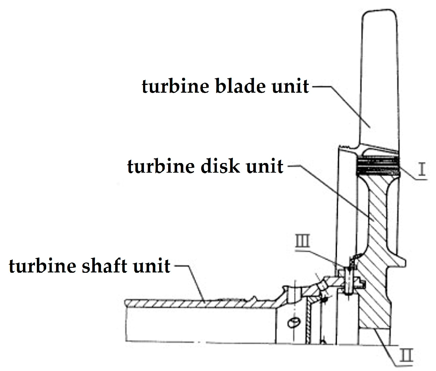
Structural units directly connected by geometric factors can transfer energy through pairs of connections. As shown in Figure 2, unit 1 is formed by the ordered combination of connection I, II, III, and rotor disk geometries, which determine the shape and size of unit 1. When unit 2 works, energy is transferred from unit 2 to unit 1 through connection III, and then from unit 1 to unit 3 through connection I, so that unit 3 works to achieve the purpose of energy transfer.
A geometric factor usually controls the synthesis of a pair of connections, and some complex connections can also be controlled by several geometric factors.
Figure 2 shows the connected attribute sets making up units. I is the connection between the turbine disk and turbine blades; II is the connection between the turbine disc and turbine shaft; III is the pin connection between the turbine disc and turbine shaft.

2.1.2. Property Family of Turbine Rotor Structural Unit

The function and properties of the engine rotor structure are determined by the element property family. The unit property family is composed of a type property set, a connection property set, and a material property set. The following formulae represent the relationship between them.
The unit property family can be expressed as Equation (2):
G e = G e t G e c G e m
where G e t is the type property set; G e c is the connection property set; G e m is the material property set.
The set of type attributes can be represented as Equation (3):
G e t = F c f , U n
where F c f is the geometric factor that controls the synthesis of G e t , the functional type of F c f can be named G e t , and U n is the unit composed of G e t .
The set of connection properties can be represented as Equation (4):
G e c = U n 1 U n 2 , F c c , A t = U n 1 U n 2 , F c c , A m V a
where U n 1 U n 2 is used to name G e c , and the set of connection attributes that make up unit 2 can be named unit 2-unit 1; F c c is a geometric factor to control the synthesis of G e c , and U n 1 is a unit composed of G e c . U n 2 is a unit directly connected to U n 1 via F c c ; A t is the constraint attribute of cell body; A m and V a are the attribute quantity set and attribute value set of A t , whose definition is the same as the constraint attribute of the geometric factors.
The set of material properties can be expressed as Equation (5):
G e m = F c m , U n
where F c m is the geometric factor that controls the synthesis G e m , G e m can be named by the functional type of F c m , and U n is the unit composed of G e m .

2.2. Geometric Coding Model of Turbine Rotor Unit

2.2.1. Geometric Encoding of Shaft Unit

The biggest characteristic of a shaft class is its length, as well as the type of shaft. Therefore, the main coding is the length control factor and the type of geometry of the shaft; the type of geometry of the shaft determines whether the shaft is a solid shaft or a hollow shaft, a straight shaft or a conical shaft. According to the type of the shaft, it can be further coded and divided to determine the inner and outer diameter coding of the shaft and the slope coding of the shaft. According to the coordination of the shaft and other parts, the position code needs to be added or the shape code of the slot holes needs to be added to the keyway on the shaft, and finally the complete shaft unit body is formed.
The proposed shaft model is coded as Equation (6):
Z 0 , Z 1 , R , r , d , α , T
where Z 0 is the initial position of the shaft growth starting point; R is the outside diameter of the shaft; r is the inner diameter of the shaft (r = 0, is the real shaft); d is the shaft length; α is the cone angle of the shaft; T is the type of connected geometry on the shaft. Z 0 , Z 1 are position constraint control factors.

2.2.2. Geometric Encoding of Disk Unit

The disk parts have the characteristics of a large radius and small thickness. The appearance of a slot on the edge of the disk and a hole in the disk can be regarded as the result of biological evolution in nature. The result of its evolution is that the geometric factor of the receiving disk structure can be coded and controlled, and the type of mortise on the disk, the inner and outer diameter of the disk, and the thickness of the disk can be controlled.
The proposed disk model is coded as Equation (7):
T m , T d , Z 0 , R , r , d , n z , α 1
Including Equations (8) and (9) in Equation (7):
T m = n g , F a , F b , Z d , β 2
T d = α 3 , r 1 , r 2
where T m is the mortise code of the disc parts; n z is the number of mortise; α 1 is the torsion angle of the disc; T m is the fir-tree mortise code, and its internal parameters n g are the number of fir-tree mortise teeth; F a and F b are the arithmetic factors of the fir-tree mortise; Z d is the position function of symmetric line of the fir-tree mortise; β 2 the inclination angle of the fir-tree mortise; T d is the type of disk (straight disk, cone disk, and edge ladder cone disk); Z 0 is the initial position of the disk growth starting point; R is the outer diameter of the disk; r is the inner diameter of the disk; d is the thickness of the disk. In the special disk type code, α 3 is the bevel of the cone disk, r 1 is the radius of the flange closest to the edge of R , and r 2 is the radius of the flange closest to the edge of r .

2.2.3. Geometric Encoding of Blade Unit

Because the rotor blade needs to fit with the mortise on the disk, there are many geometric factors, and the shape and function control factors are mainly the parameter coding of the blade body and the parameter coding of the top of the tenon.
The proposed disk model is coded as Equation (10):
Z 0 , R , d s , n z , T b , s 1 , s 2 , H b , m , k , t , c , F d , d b , α 4 , α 5
where Z 0 is the initial position of the blade starting point; R is the position constraint control factor of tenon length; d s is the thickness of the tenon and n z is the number of rotor blades; T b is the type of rotor blade, which is similar to the mortise code of the disk model; s 1 is the protruding length of the top of the tenon; s 2 is the top width of the tenon; H b is the blade height; m , k , t and c are blade shape parameters; F d is the blade shape amplification factor; d b is the blade thickness; α 4 is the mortise twist angle; α 5 is the blade body twist angle.

3. Methods

3.1. Modeling Algorithm for Rotor Shaft Unit Point Cloud Model

3.1.1. The Type Attribute Set of the Shaft

1.
Two-dimensional point cloud modeling algorithm for shafts.
Two-dimensional point cloud data of the shaft model can be obtained according to R , r in the axial geometry coding model. The algorithms are as Equations (11) and (12).
B x i = r cos c B y i = r sin c
B x j = R cos c B y j = R sin c
where B is the shaft of the boundary data storage array, i is 0, 1, 2, …, n ; j is n + 1 , n + 2 , …, n + m ; array holds the x, y coordinates and RGB color values of the shaft boundaries; c is an angular variable in increments of 0.1 from 0 to 360 degrees.
The scan-line filling algorithm is based on the region fill algorithm, which is based on the vector form data of polygonal borders and can be used for program fill or interactive fill. The specific implementation methods in MFC are as follows: CreatePolygonRgn function is used to determine the polygon boundary region through scanning line filling, PtInRegion function is used to scan and judge the data in the boundary region, and then assign values according to the definition. The point cloud data are saved to the array D D x , D y , D r g b , which stores the coordinate information of x and y of the two-dimensional cross-section of the shaft, as well as the defined pixel color information.
2.
Three-dimensional point cloud modeling algorithm for shafts.
According to d , α of the control factors in the type of geometry, a three-dimensional point cloud array T with basic shaft can be obtained. The two-dimensional point cloud data on the constant section of the direct shaft are basically unchanged, and only the control factor d controlling the length of the shaft is available. The algorithm is as Equation (13):
T x i + 1 = T x i T y i + 1 = T y i T z i + 1 = T z i + δ
when i takes 0, 1, 2, …, n, T z n T z 0 = d . where δ is the increment in the direction of the z axis and T z n is the last z coordinate value of T .
The cone shaft has a similar cross-section in the xy plane and is reduced or enlarged in the z-shaft direction. The formation of the cone shaft depends on the control factor α controlling the cone angle and the control factor d controlling the shaft length. The algorithm is shown in the following Equation (14):
T x i + 1 = T x i 2 + T y i 2 + δ tan α cos arctan T y i T x i T y i + 1 = T x i 2 + T y i 2 + δ tan α sin arctan T y i T x i T z i + 1 = T z i + δ
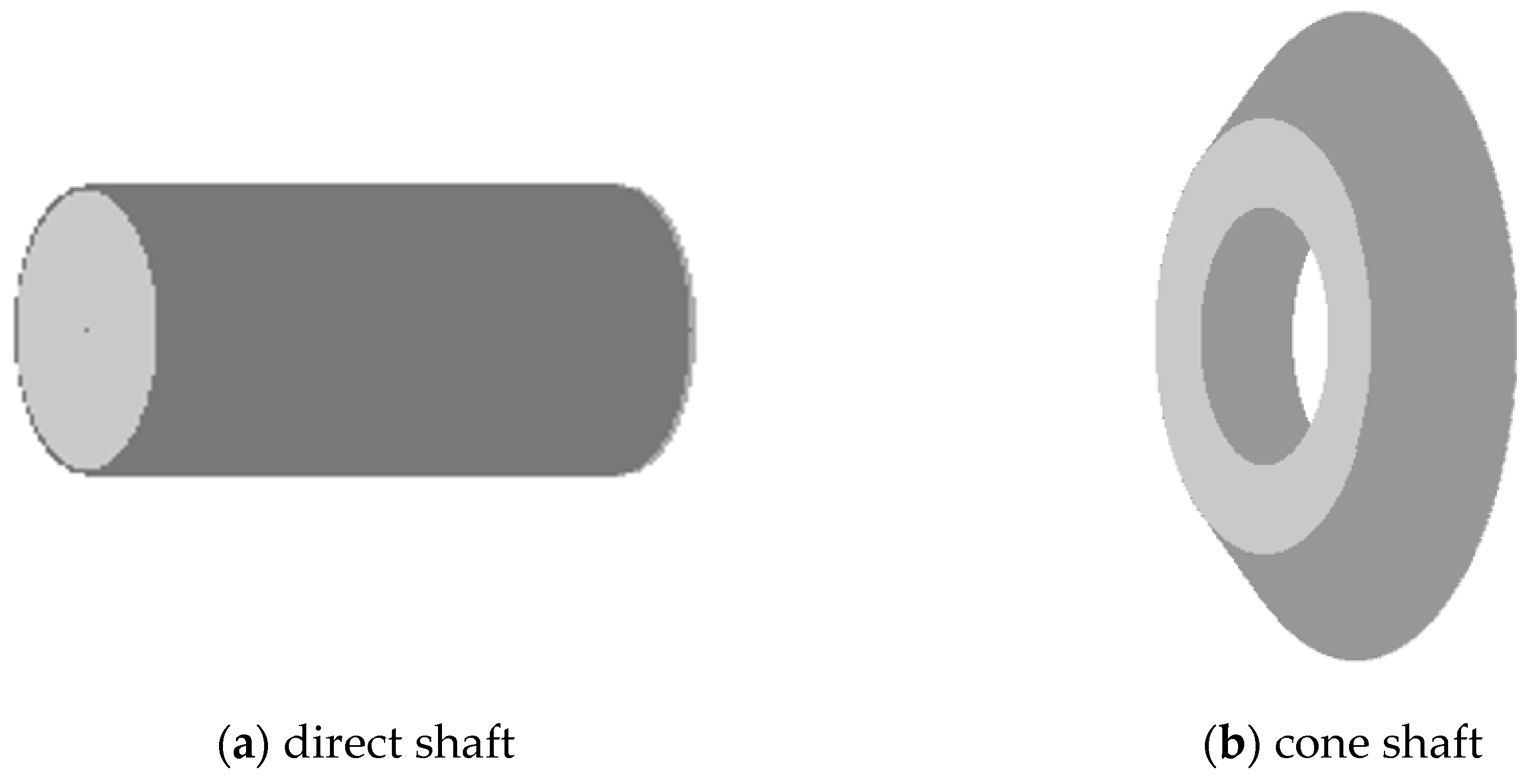
Through the above algorithm, the basic three-dimensional point cloud data T T x , T y , T r g b of the shaft, are obtained, as shown in Figure 3.

3.1.2. The Connection Attribute Set of the Shaft

The connecting attribute set of the shaft includes key holes, shaft shoulders, and pin holes. Geometric factors need to be added to model key holes, shoulder, and pin holes. The geometric factor of the keyway is Z 01 , h , b , L , h z , n z and the geometric factor of the pin is Z 02 , r z , h z , n z . The geometric factor of material geometry is E , α , ρ .
3.
Keyway generation.
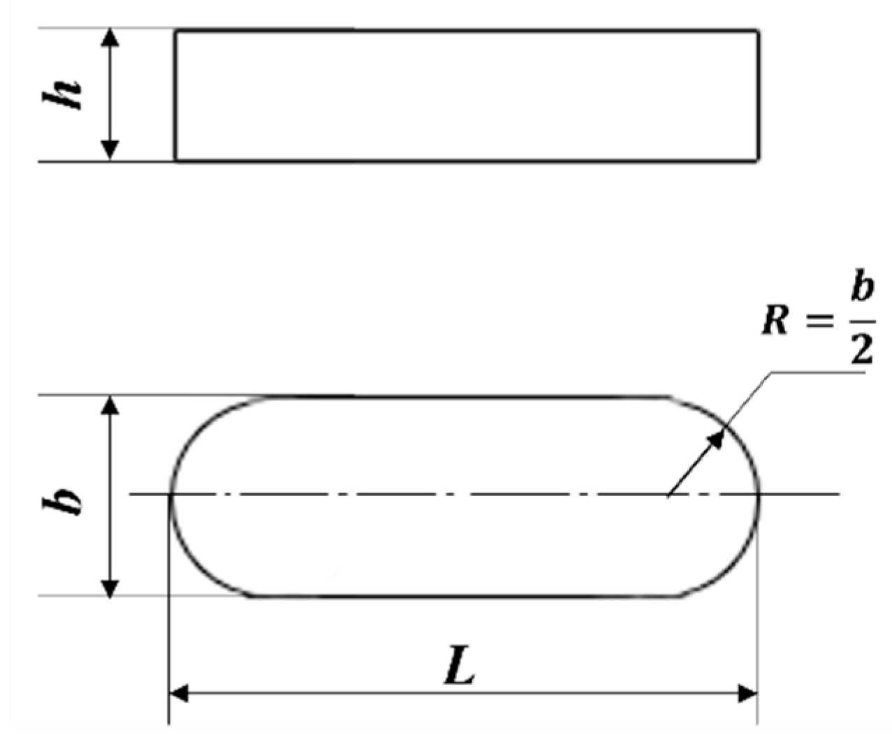
According to the keyway geometric factors Z 01 , b , L , h z , n z , a three-dimensional point cloud model T 1 of the keyway can be created. Z 01 is the position constraint geometric factor of the axial slot, b is the width of the keyway, and L is the length of the keyway. These control factors control the basic shape of the keyway as shown in Figure 4; h z controls the depth of the keyway, and n z can control the number of the keyways in the shaft.
It is necessary to design the algorithm of the arc segment and the straight segment and store the fourth boundary data for the 2D boundary modeling of the keyway.
The algorithm for the first arc is as Equation (15):
B 1 x i = b 2 cos c B 1 y i = b 2 sin c
where c is an angle variable with an increment of 0.1 from 90 to 270 degrees, and i is 0, 1, 2, …, n .
For the second straight line, the algorithm is as Equation (16):
B 1 x j = δ B 1 y j = b 2
where δ is the length variable from 0 to L b with increments of 0.1, j is n + 1 , n + 2 , …, n + m .
The algorithm for the third arc is as Equation (17):
B 1 x k = b L + b 2 cos c B 1 y k = b 2 sin c
where c is an angular variable with an increment of 0.1 from 270 to 360 degrees, and k is n + m + 1 , n + m + 2 , …, n + m + o .
For the fourth straight line, the algorithm is as Equation (18):
B 1 x l = b L + δ B 1 y l = b 2
where δ is the length variable from 0 to L b with increments of 0.1, l is n + m + o + 1 , n + m + o + 2 , …, n + m + o + p .
After obtaining the point cloud data of the boundary of the keyway, the internal data are filled. Similar to the internal fill of the shaft, CreatePolygonRgn function and PtInRegion function are used to obtain the internal boundary array D 1 D 1 x , D 1 y , D 1 r g b .
In actual engineering, the generation of a keyway is formed on the shaft by a milling cutter, which is the same in the program. The generation of keyway data needs to be modified in the three-dimensional point cloud data T T x , T y , T r g b of the shaft. Coordinate transformation of point cloud data D 1 D 1 x , D 1 y , D 1 r g b is required in the calculation process, and the specific algorithm is as Equation (19):
T x i = δ 1 T y i = D 1 y i T z i = Z 01 + D 1 x i
where δ 1 ranges from 0 to h z , with an increment of 0.1. The algorithm converts the keyway cross section drawn on the xy plane to the yz plane through coordinates, and then assigns values to the negative direction of the x shaft continuously. RGB is defined as the same value as the background RGB (255, 255, 255), thus completing the “milling” operation. The 3D point cloud data with keyway shaft are obtained as T T x , T y , T r g b .
4.
Generation of pin holes.
A three-dimensional point cloud model of pin holes can be created according to the pin hole geometric factors Z 02 , r z , h z , n z . Z 02 is the constraint control factor of the position of the pin holes in the axial direction, r z is the radius of the hole, h z is the hole depth, and n z can control the number of evenly divided pin holes in the circumferential direction of the shaft.
The two-dimensional boundary algorithm of the pin hole is as Equation (20):
B 2 x i = r z cos c B 2 y i = r z sin c
where c is the angle variable in 0 to 360 degree increments of 0.1.
The filling of the point cloud data inside the pin hole is like the filling of the shaft inside. The CreatePolygonRgn function and PtInRegion function are used to obtain the inner boundary data D 2 D 2 x , D 2 y , D 2 r g b .
For a shaft that requires n z pin holes, the pin hole data need to be copied, and the algorithm is as Equation (21):
D 2 x i = D 2 x i cos 2 π j n z D 2 y i sin 2 π j n z D 2 y i = D 2 x i sin 2 π j n z + D 2 y i cos 2 π j n z
where D 2 D 2 x , D 2 y , D 2 rgb , are the replicated pin hole point cloud data, j is 1, 2, …, n z .
In actual engineering practice, the generation of pin holes is formed by drilling holes on the shaft, which is also the case in the program. The generation of pin hole data needs to be modified in the three-dimensional point cloud data T T x , T y , T r g b of the shaft. In the calculation process, coordinate transformation of point cloud data D 2 D 2 x , D 2 y , D 2 r g b is required, and the specific algorithm is as Equation (22):
T x i = δ 1 T y i = D 2 y i T z i = Z 02 + D 2 x i
In the formula, δ 1 ranges from 0 to h z with an increment of 0.1. The algorithm converts the cross section of the pin hole drawn on the xy plane to the yz plane through coordinates, and then assigns a value to the negative direction of the x shaft continuously. RGB is defined as the same value as the background RGB (255, 255, 255), and then completes the operation of “drilling”. The 3D point cloud data with pin hole shaft are T T x , T y , T r g b .
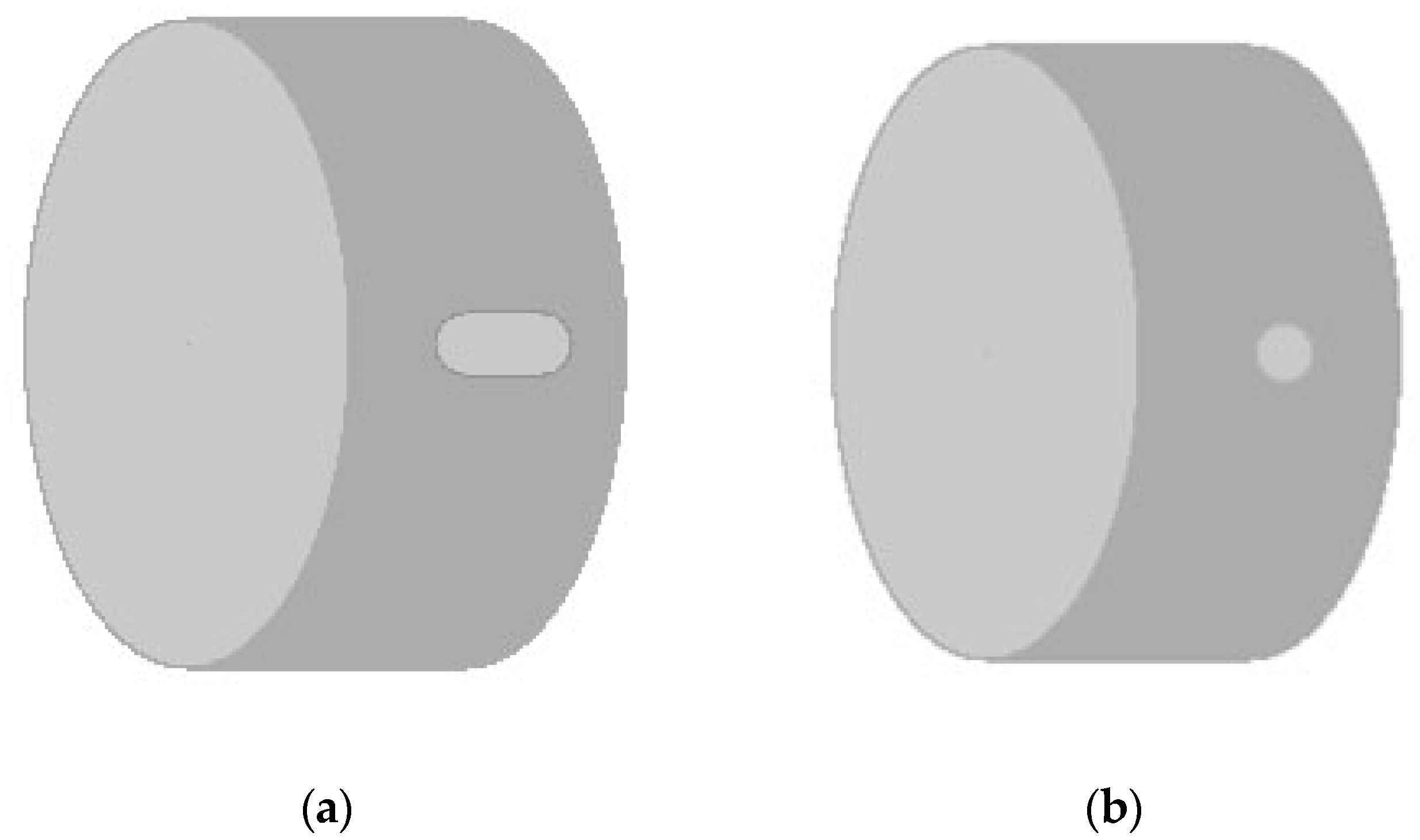
In summary, the shaft point cloud data generation diagram with keyway and pin hole is shown in Figure 5.

3.1.3. The Material Attribute Set of the Shaft

According to the People’s Republic of China aviation industry standard HB20082-2012 “Aviation high-temperature alloy shaft forging specification” the selected material geometry are alloy steel GH2901, GH4169, and GH4500 [17], The controlling factor of the material geometry is E , α , ρ . E is the elastic modulus; α is the coefficient of linear expansion, and ρ is the density. The control factors for these three materials are shown in Table 1.

3.2. Modeling Algorithm for Rotor Disk Unit Point Cloud Model

3.2.1. The Type Attribute Set of the Disk

Turbine disk can be based on fir-tree mortise. Its coding chain model is n g , F a , F b , Z d , β 2 , α 3 , r 1 , r 2 , Z 0 , R , r , d , n z , α 1 . Its modeling algorithm is as follows:
5.
2D point cloud modeling algorithm for turbine disk;
Boundary point cloud data B B x , B y , B r g b of turbine disk can be obtained according to the control factor R , r , and the algorithm are as Equations (23) and (24).
B x i = r cos c B y i = r sin c
B x j = R cos c B y j = R sin c
where B is the boundary data storage array of disk; i = 0, 1, 2, …, n ; j is n + 1 , n + 2 , …, n + m ; c is an angular variable in increments of 0.1 from 0 to 360 degrees.
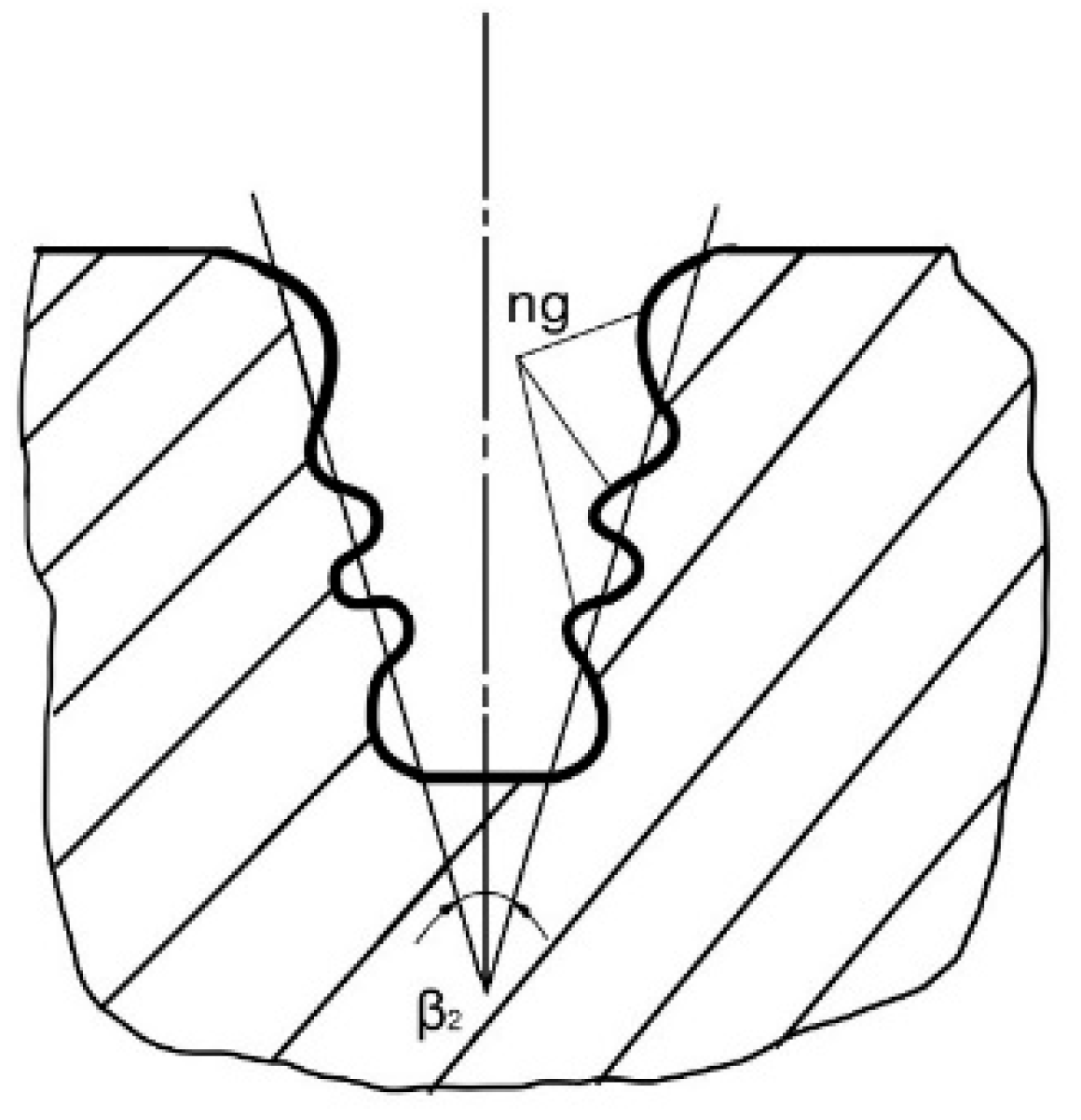
After obtaining the boundary data B B x , B y , B r g b , further fill the interior to obtain two-dimensional point cloud data D D x , D y , D r g b of the disk. The point cloud data of the Fir-tree mortise and tenon is created on the two-dimensional point cloud data D D x , D y , D r g b of disk. According to the control factor n g , F a , F b , Z d , β 2 of the Fir-tree mortise and tenon, some parameters of the mortise and tenon need to be calculated first, as shown in Figure 6.
The algorithm for the first fir tooth can be expressed by Equations (25)–(27):
O x = n g + 0.3 F b π
O y = Z d
B 1 x i = O x + δ cos β 2 F a sin 2 δ F b sin β 2 B 1 y i = Z d δ sin β 2 F a sin 2 δ F b cos β 2
In the formula, O x and O y are the initial position of the fir-tree slot, which is determined by the position constraint factor. i = 0, 1, 2, …, n ; δ is the length variable from 0 to O x in increments of −0.01.
For the second straight line, the algorithm is as Equation (28).
B 1 x j = B 1 x n B 1 y j = δ
where j is n + 1 , n + 2 , …, n + m ; δ is a length variable with increments of 0.1 from B 1 y n to B 1 y n .
The algorithm for the third fir tooth is as Equation (29).
B 1 x k = B 1 x n i B 1 y k = B 1 y n i
where k is n + m + 1 , n + m + 2 , …, n + m + o ; i take 1, 2, …, n .
For the fourth straight line, the algorithm is as Equation (30).
B 1 x l = B 1 x n + m + o B 1 y l = δ
where l is n + m + o + 1 , n + m + o + 2 , …, n + m + o + p ; δ is the length variable of B 1 y n + m + o through B 1 y n + m + 0 increments of −0.1.
At this point, the two-dimensional boundary data modeling of a single fir-tree slot is completed, and the internal points are saved to D 1 D 1 x , D 1 y , D 1 r g b by using the internal filling algorithm. The two-dimensional point cloud data of a single fir-tree tenon is arranged in n z equal parts of the circumference by the rotation replication algorithm, and the algorithm is as Equation (31).
D 2 x i = D 1 x i cos 2 π j n z R + D 1 y i sin 2 π j n z D 2 y i = D 1 x i sin 2 π j n z + R + D 1 y i cos 2 π j n z
where D 2 is the two-dimensional point cloud data of n z fir-tree slots; i = 0, 1, 2, …, n ; j take 1, 2, …, n z ; R is the outer diameter of the disk.
Replace the internal data of D 2 D 2 x , D 2 y , D 2 r g b with, D D x , D y , D r g b , The point cloud data of n z fir-tree tenon on two-dimensional turbine disk D D x , D y , D rgb can be obtained.
6.
3D point cloud modeling algorithm for turbine disk;
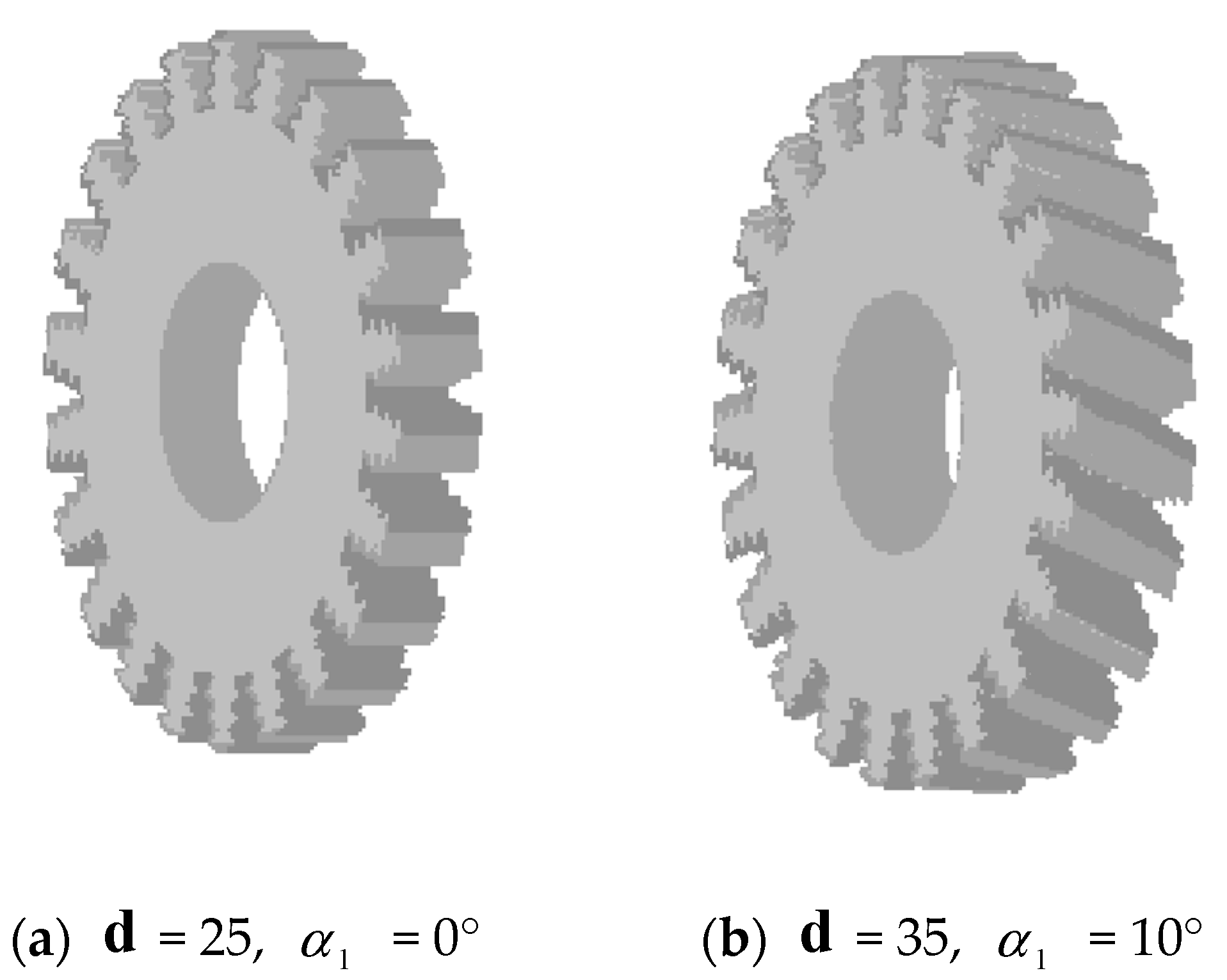
By setting the control factor d , α 1 , d can set the thickness of turbine disk; α 1 can set the inclination Angle of the tenon in the z direction. Three-dimensional point cloud data T T x , T y , T r g b of turbine disk, and the modeling algorithm is as Equation (32).
T x i = D x i cos α 1 δ d D y i sin α 1 δ d T y i = D x i sin α 1 δ d + D y i cos α 1 δ d T z i = δ
where δ is the length variable from 0 to d in increments of 0.1.
3D point cloud data T T x , T y , T r g b of turbine disk, model is shown in Figure 7.

3.2.2. The Connection Attribute Set of the Disk

The connection attribute set of the turbine disk includes cooling holes and installation edges. Control factors need to be added to model the cooling holes and installation edges. The control factor for the cooling hole is Z x , Z y , r z , n z 2 , and the control factor for the installation edge on the disc is Z 01 , R , r , n r 1 , n x , n z 1 .
7.
Cooling hole point cloud modeling algorithm
According to the control factor Z x , Z y , r z , n z 2 , after the creation of the 2D point cloud data D D x , D y , D r g b of the rotor disk class is completed, further point cloud data creation of the cooling holes can be carried out. The algorithm is as Equation (33).
B 3 x i = Z x + r z cos c B 3 y i = Z y + r z sin c
where B 3 represents the storage array of boundary data for a single cooling hole; i takes 0, 1, 2, …, n ; c is an angle variable with an increment of 0.1 from 0 to 360 degrees. Fill in and define the point cloud data within the boundary and save it to obtain the two-dimensional point cloud data D 1 D 1 x , D 1 y , D 1 r g b of the cooling holes for a single hole.
Arrange the cooling holes in a circle of n z r on the disk circumference, and the algorithm is as Equation (34).
D 2 x i = D 1 x i cos 2 π j n z r D 1 y i sin 2 π j n z r D 2 y i = D 1 x i sin 2 π j n z r + D 1 y i cos 2 π j n z r
where D 2 represents the 2D point cloud data of n z r cooling holes; i take 0, 1, 2, …, n ; j take 1, 2, …, n z r .
According to the control factor d of the rotor disc class, the three-dimensional point cloud data T T x , T y , T r g b of the cooling hole can be further obtained, and the algorithm is as Equation (35).
T x i = D 2 x i T y i = D 2 y i T z i = δ
where i is taken as 0, 1, 2, …, n ; δ is a length variable with increments of 0.1 from 0 to d .
8.
Installation edge point cloud modeling algorithm for disks;
The edge point cloud modeling algorithm installed on the disk is like the shaft, and there are two types of algorithms: one is a hollow circular tube like the shaft, and the other is a through hole disk structure like the disk. By combining the two point cloud modeling algorithms, the edge point cloud model installed on the turbine disk can be modeled, which will not be repeated here.

3.2.3. The Material Attribute Set of the Disk

The selected material geometries include iron-based high-temperature alloy GH3030, nickel based deformed high-temperature alloy GH4169, and nickel-based cast high-temperature alloy IN718. The control factor for the material geometry is E , α , ρ , E is the elastic modulus; α is the coefficient of linear expansion, and ρ is the density. The control factors for these three materials are shown in Table 2.

3.3. Modeling Algorithm for Rotor Blade Unit Point Cloud Model

3.3.1. The Type Attribute Set of the Blade

The rotor blade is connected to the mortising groove on the disk, and its 3D point cloud data are complicated. When conducting 3D point cloud data modeling, rotor blades are divided into tenons and blade segments according to their structure, and the main difference between turbine blades is the twist angle and tenon of the blade body. Therefore, the coding chain model of turbine blades is as follows: Z 0 , R , d , α 1 , n z , n g , F a , F b , Z d , β 2 , S 1 , S 2 , d s , m , k , t , c , F d , H b , α 4 , α 5 .
9.
Modeling algorithm for tenon point cloud model.
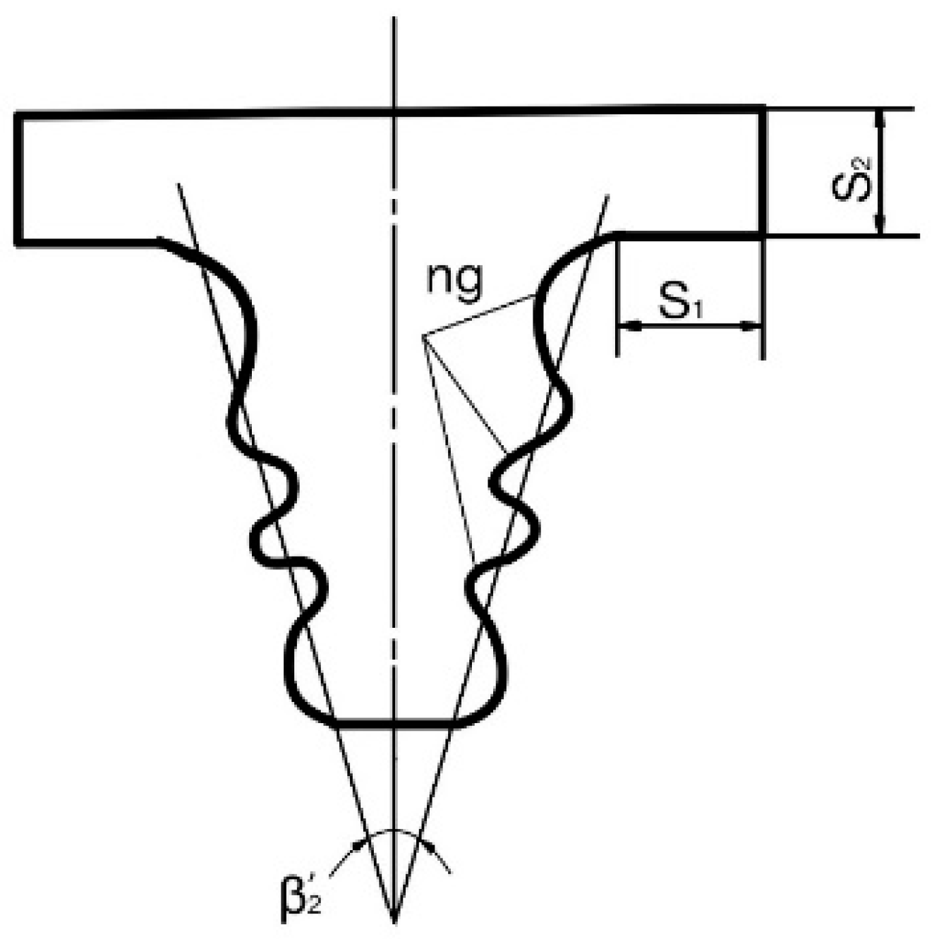
Because the tenon needs to fit with the compressor disk or turbine disk, the tenon groove on the point cloud model is similar to that on the disk. One just has to adjust the control factors n g , F a , F b , Z d , β 2 , S 1 , S 2 , d s to complete the tenon point cloud model creation.
According to the control factor n g , F a , F b , Z d , β 2 , S 1 , S 2 , d s , fir-tree tenon boundary point cloud data B 2 B 2 x , B 2 y , B 2 r g b can be created. The schematic diagram of the fir-tree tenon is shown in Figure 8.
Due to the similarity between the 2D point cloud model algorithm of the blade fir-tree tenon and the 2D point cloud model algorithm of the disk fir-tree tenon groove, it will not be elaborated further.
10.
Modeling algorithm for blade body point cloud model.
The most important part of the blade body is the blade profile parameter. The modeling rule refers to the quadratic curve method. The idea is to first determine the curvature line y c and the thickness line y t , and then combine the two to draw the blade profile. The bending line is divided into two sections, namely, the first half y c 1 and the second half y c 2 . Two corners θ 1 and θ 2 are designed in the bending line. The specific implementation algorithm can be expressed as Equations (36)–(40):
y c 1 x 0 = c k 6 x 0 3 3 m x 0 2 + m 2 x 0 3 m
y c 2 x 0 = c k m 3 6 1 x 0
y t x 0 = 5 c t 0.2969 x 0 0.126 x 0 0.3516 x 0 2 + 0.2843 x 0 3 0.1034 x 0 4
θ 1 x 0 = arctan d y c 1 d x 0 = arctan c k 6 3 x 0 2 6 m x 0 + 3 m 2 m 3
θ 2 x 0 = arctan d y c x d x 0 = arctan c k m 3 6
where c is the string length; k is the maximum relative camber; m c is the position of maximum thickness. t is the maximum relative thickness; The value of x 0 ranges from 0 to c .
The blade profile function is obtained.
The algorithm for the first curve is as Equation (41):
u = x 0 y t x 0 sin θ 1 x 0 v = y c 1 x 0 + y t x 0 cos θ 1 x 0
where ( u , v ) is the first blade curve coordinate, and the value of x 0 is from 0 to m c .
The algorithm for the second curve is as Equation (42):
u = x 0 y t x 0 sin θ 2 x 0 v = y c 2 x 0 + y t x 0 cos θ 2 x 0
where ( u , v ) is the curvilinear coordinate of the second blade profile, and the value of x 0 is from m c to c .
The algorithm for the third curve is as Equation (43):
u = x 0 + y t x 0 sin θ 2 v = y c 2 x 0 y t x 0 cos θ 2
where ( u , v ) is the curvilinear coordinate of the third segment of the blade profile, and the value of x 0 is from m c to c .
The algorithm for the fourth curve is as Equation (44):
u = x 0 + y t x 0 sin θ 1 v = y c 1 x 0 y t x 0 cos θ 1
where ( u , v ) is the curvilinear coordinate of the fourth segment of the blade profile, and the value of x 0 is from 0 to m c .
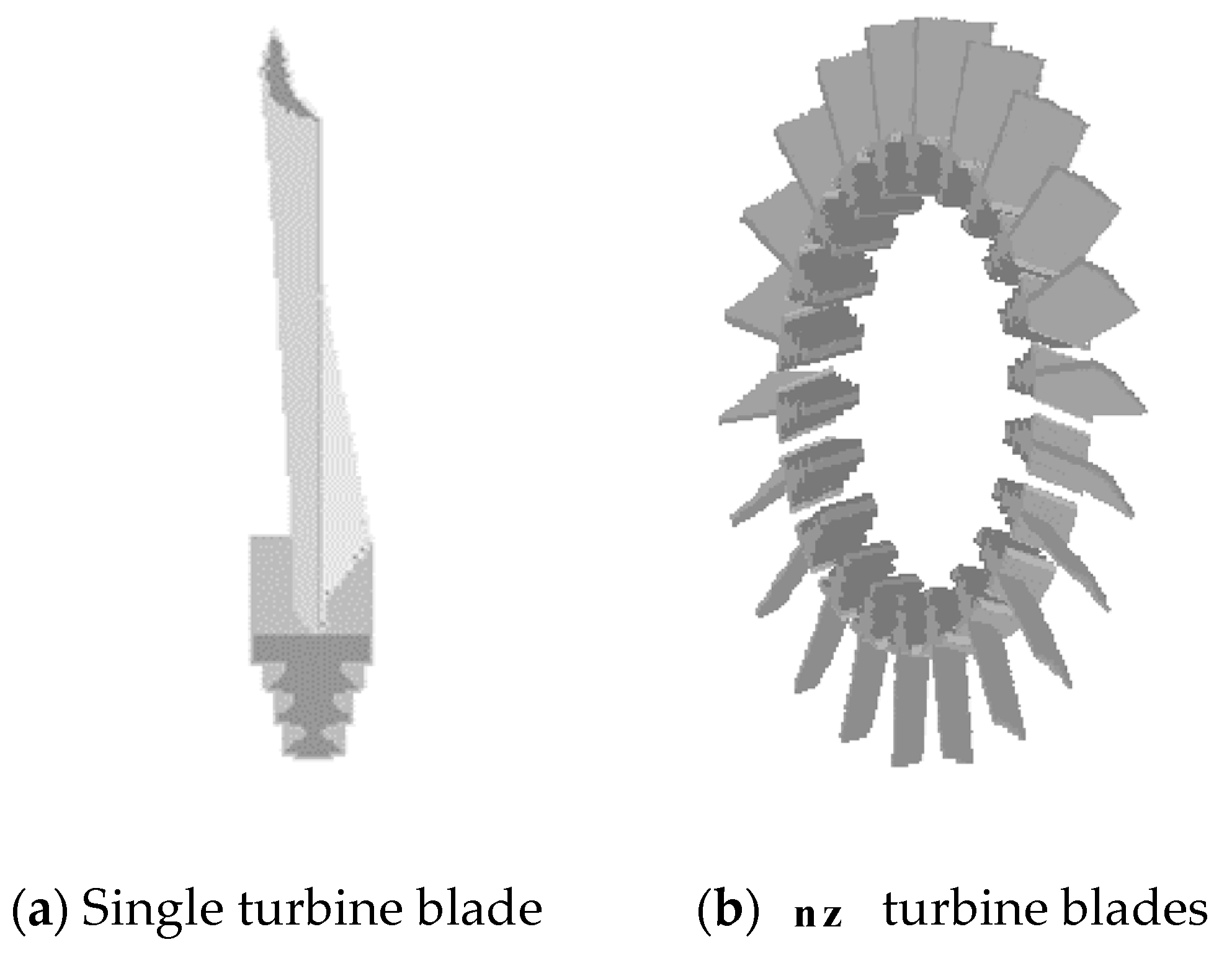
Therefore, the blade profile boundary can be modeled by adjusting the blade profile control factor m , k , t , c , F d , H b , α 4 , α 5 . According to the above algorithm, the blade profile boundary D D x , D y , D r g b can be obtained. Since the blade body is not straight on the tenon, the rotation angle of the blade profile on the tenon is controlled by the control factor α 4 , the algorithm is as Equation (45):
B x i = B x i cos α 4 B y i sin α 4 B y i = B x i sin α 4 + B y i cos α 4
After rotating the blade profile boundary B B x , B y , B rgb , the internal point filling algorithm can be used to obtain the two-dimensional blade point cloud model data D D x , D y , D r g b . Finally, the control factors H b and α 5 are used to obtain the three-dimensional point cloud data T T x , T y , T r g b model of the rotor blade. The algorithm is as Equation (46):
T x i = δ T y i = D x i sin α 5 δ H b + D y i cos α 5 δ H b T z i = D x i cos α 5 δ H b D y i sin α 5 δ H b
where δ is the length variable from 0 to H b in increments of 0.1.
The generated 3D point cloud model image is shown in Figure 9.

3.3.2. The Connection Attribute Set of the Blade

The connection attribute set of the turbine blades has a wide variety of types and the structure is too complex to be studied in this article.

3.3.3. The Material Attribute Set of the Blade

The rotor blades are mainly made of titanium alloy, titanium matrix composite material, and superalloy blades in the compressor section. In the turbine section, nickel-based and nickel–Al-based superalloy titanium–aluminum alloy blades and ceramic-based composite blades are mainly cast. The controlling factors of the material geometry are E , α , ρ , E is the elastic modulus; α is the coefficient of linear expansion, and ρ is the density. The control factors of these three materials are shown in Table 3.

4. Results and Discussion

4.1. Display of 3D Point Cloud Model Data Results in MFC

The essence of MFC is a library containing many objects that have been defined by Microsoft. Through it, programmers can efficiently develop a variety of applications based on the Windows operating system.
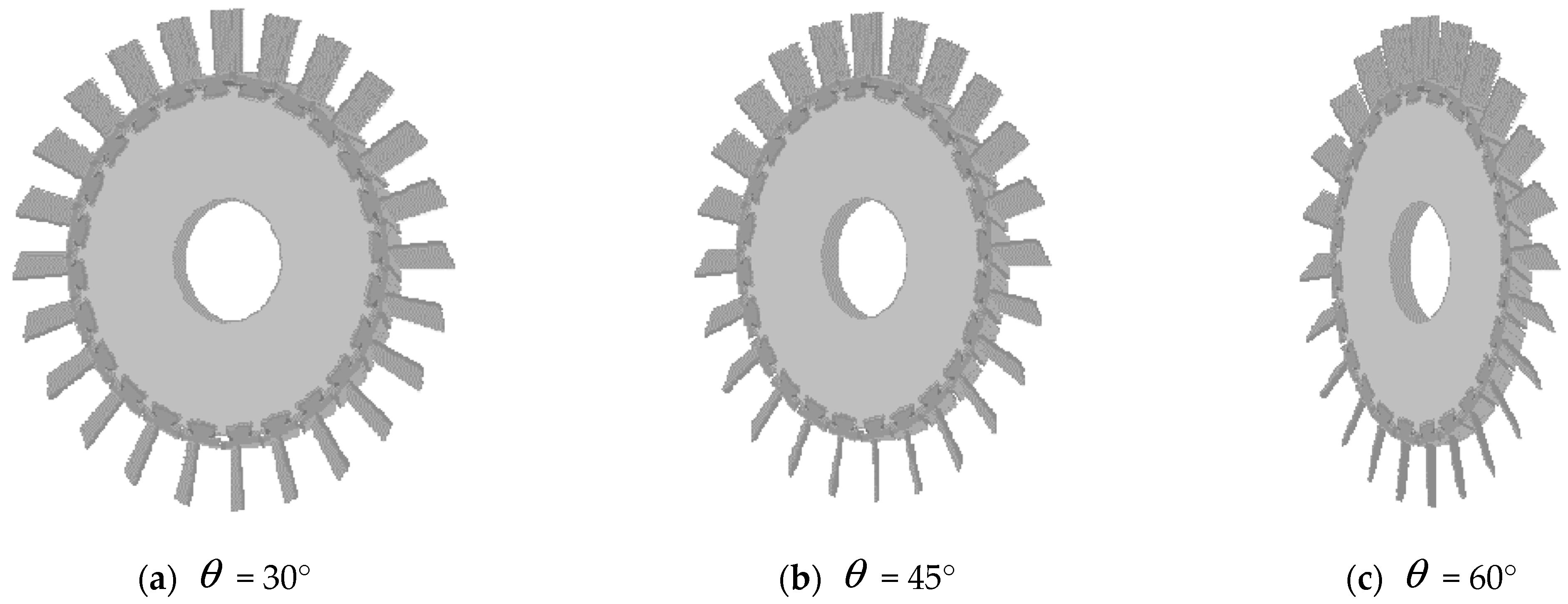
The realization of the point cloud model on MFC only needs to have obtained all the three-dimensional coordinate points of the model, draw the customer area of the application window through OnDraw(CDC*pDC) function, and display the obtained entity three-dimensional coordinate points using SetPixel function. In the MFC window display rule of vs, only two-dimensional images x and y can be displayed. The control factor θ can be changed by three-dimensional coordinate transformation, and the three-dimensional display angle of geometry can be adjusted, as shown in Figure 10. The algorithm is as Equation (47):
T x i = T x i cos θ T z i sin θ T y i = T y i
where T x i and T y i are the position coordinates of the cell model displayed in the MFC window; δ take 0, 1, 2, …, n ; θ shows the angle for the cell body in the window.

4.2. Units Coordination Display

A variety of geometry 3D point cloud models will produce display interference when displaying or when display is incomplete. The main reason is that due to the sequence of geometry display algorithms, after the completion of the 3D display of a geometry, if the next geometry needs to be displayed, the former geometry may be covered by the 3D display model of the latter geometry. To solve this problem, inspired by the bounding box algorithm for surface intersection, the 3D point cloud data of geometry are no longer saved according to the sequence of data. They are arranged according to the bounding box data sequence; a bounding box is placed to store the geometry that needs to be displayed, and then the bounding box is displayed, and the coordinate information of the data points and the display color information are saved under the numbering order. The algorithm is as Equation (48):
Z T T x i + X 2 + X T y i + Y 2 + X Y T z i + Z 0 x = T x i Z T T x i + X 2 + X T y i + Y 2 + X Y T z i + Z 0 y = T y i Z T T x i + X 2 + X T y i + Y 2 + X Y T z i + Z 0 z = T z i + Z 0 Z T T x i + X 2 + X T y i + Y 2 + X Y T z i + Z 0 R = T R i Z T T x i + X 2 + X T y i + Y 2 + X Y T z i + Z 0 G = T G i Z T T x i + X 2 + X T y i + Y 2 + X Y T z i + Z 0 B = T B i
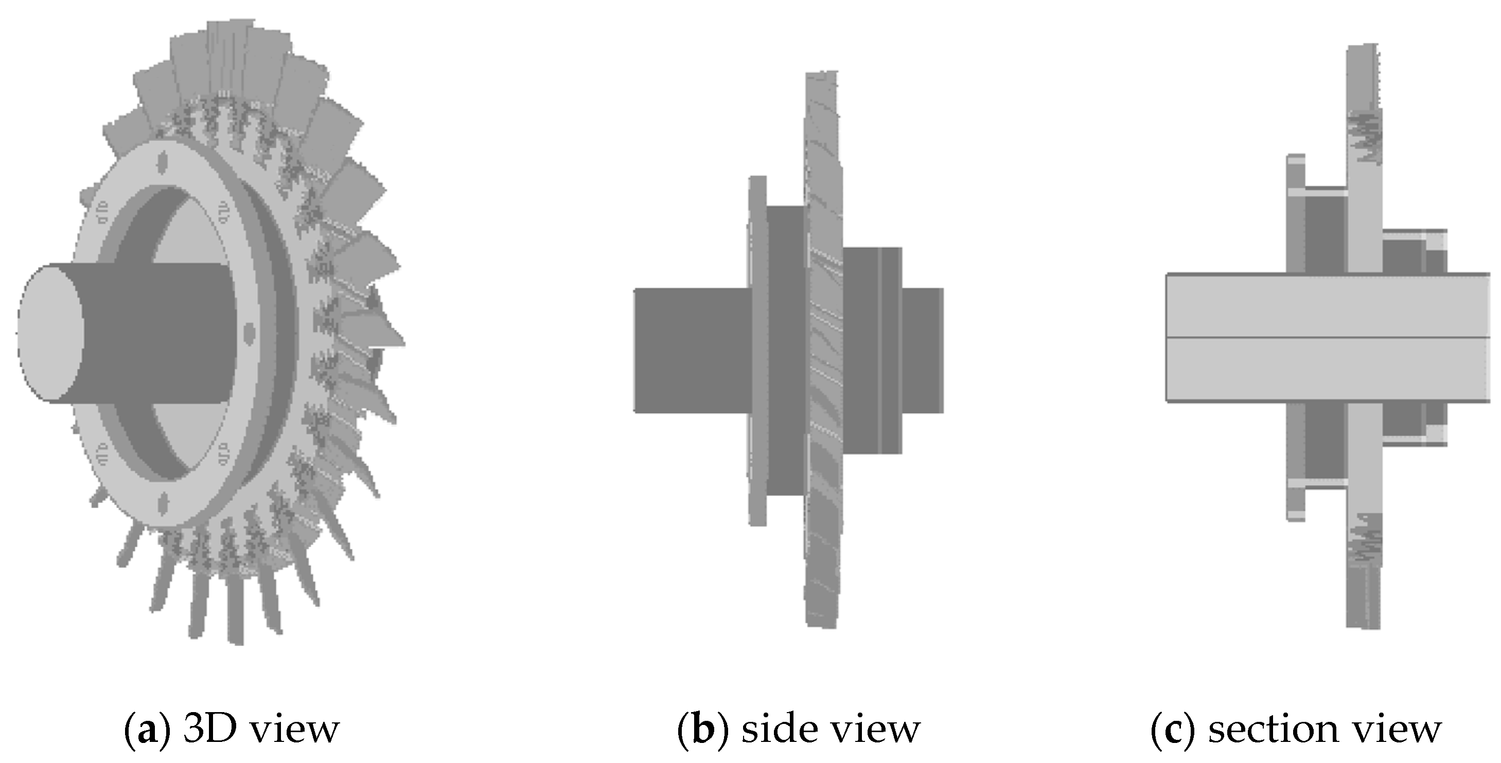
where X , Y , Z is the size of the bounding box, T T x , T y , T r g b is the three-dimensional point cloud array of the cell body; Z T Z T x , Z T y , Z T z , Z T r g b is the three-dimensional point cloud array of the cell body displayed inside the bounding box. The 3D display improved by this algorithm is shown in Figure 11.

5. Conclusions

This paper presents a geometric coding method for aeroengine turbine rotor structure and introduces a computer graphics point cloud model display algorithm. The proposed method is based on geometric coding technology, which mainly encodes turbine structures. These geometric codes are related to the design parameters of turbine structures. The codes are based on geometric structures and have certain universality and independence. In the model study of this paper, once the coding is determined and the parameters of each geometric control factor are known, the point cloud model of the turbine rotor structure can be generated, which is equivalent to the inverse transformation of the coding. The resulting point cloud model data body is prepared in advance for later visualization of the point cloud model. In general, the computational efficiency of the coding model algorithm and the reconstruction of the point cloud model are very good, although more points need to be calculated. In addition, the more complex the turbine rotor model is, the more the geometric control factor parameters will be increased, thus increasing the detail level of the turbine rotor model structure. On the other hand, when displaying the turbine rotor point cloud model, inspired by the bounding box algorithm, the interference display problem existing in the sequential display of turbine rotor units is solved, and multiple unit models can be assembled and displayed normally. Finally, the coding provided to the machine learning algorithm will save design time for the structure design of aeroengine turbines, and have a reference value for the structure design of aeroengine turbines.

Author Contributions

Conceptualization, W.X. and H.L.; methodology, W.X.; software, L.Z.; validation, W.X., B.H. and H.L.; formal analysis, L.Z.; investigation, H.L. and W.X.; resources, W.X.; data curation, W.X. and L.Z.; writing—original draft preparation, W.X. and H.L.; writing—review and editing, W.X., H.L., L.Z. and B.H.; visualization, W.X.; supervision, W.X.; project administration, W.X.; funding acquisition, H.L. All authors have read and agreed to the published version of the manuscript.

Funding

This research was funded by the Natural Science Foundation of Jiangxi Province, grant number 20201BBE51002.

Data Availability Statement

Data are contained within the article.

Conflicts of Interest

The authors declare no conflict of interest.

References

  1. Wang, Y. Research on Intelligent CAD Innovation Design Based on Biological Genes. Master’s Thesis, Northwestern Polytechnical University, Xi’an, China, 2003. [Google Scholar]
  2. Li, N.; Bu, S.; Shang, B.; Li, Y.; Tang, Z.; Zhang, W. Vision and Key Issues of Intelligent Aircraft Design. J. Chin. J. Aeronaut. 2021, 42, 213–230. [Google Scholar]
  3. Behbahani, A.; Tulpule, B. Perspective for distributed intelligent engine controls of the future. In Proceedings of the 46th AIAA/ASME/SAE/ASEE Joint Propulsion Conference & Exhibit, Nashville, TN, USA, 25–28 July 2010; p. 6631. [Google Scholar]
  4. Rosenman, M.A. An exploration into evolutionary models for non-routine design. J. Artif. Intell. Eng. 1997, 11, 287–293. [Google Scholar] [CrossRef]
  5. Ming, D. Principles and Construction of Aviation Gas Turbine Engines; National Defence Industry Press: Beijing, China, 2008; pp. 2–3. [Google Scholar]
  6. Kraev, V.M.; Siluyanova, M.V.; Tikhonov, A.I. Assessment and improvement of rationality methods of modern aircraft engines design and technological solution. J. Phys. Conf. Ser. 2019, 1353, 012–033. [Google Scholar] [CrossRef]
  7. Wang, H. Parameterized Design, Analysis and Software Integration of Turbine Rotor Structure. Master’s Thesis, Nanjing University of Aeronautics and Astronautics, Nanjing, China, 2005. [Google Scholar]
  8. Cao, J. Research on the Life Assessment Method of Aircraft Engine Turbine Rotors. Master’s Thesis, Harbin Institute of Technology, Harbin, China, 2015. [Google Scholar]
  9. Collopy, P.D.; Hollingsworth, P.M. Value-driven design. J. Aircr. 2011, 48, 749–759. [Google Scholar] [CrossRef]
  10. Tammineni, S.V.; Rao, A.R.; Scanlan, J.P.; Reed, P.A.S.; Keane, A.J. A knowledge-based system for cost modelling of aircraft gas turbines. J. Eng. Des. 2009, 20, 289–305. [Google Scholar] [CrossRef]
  11. Curran, R.; Raghunathan, S.; Price, M. Review of aerospace engineering cost modelling: The genetic causal approach. J. Prog. Aerosp. Sci. 2004, 40, 487–534. [Google Scholar] [CrossRef]
  12. Weustink, I.F.; Ten Brinke, E.; Streppel, A.H.; Kals, H.J.J. A generic framework for cost estimation and cost control in product design. J. Mater. Process. Technol. 2000, 103, 141–148. [Google Scholar] [CrossRef]
  13. Xiao, R. Principles and Technologies of Intelligent Design; Science and Technology Press: Beijing, China, 2006; pp. 14–15. [Google Scholar]
  14. Reding, D.F.; Eaton, J. Science & Technology Trends 2020–2040. Exploring the S&T Edge; NATO Science & Technology Organization: La Spezia, Italy, 2020; pp. 71–73. [Google Scholar]
  15. Freeman, H. On the encoding of arbitrary geometric configurations. J. IRE Trans. Electron. Comput. 1961, 260–268. [Google Scholar] [CrossRef]
  16. Tianjue, G. Biochemistry; People’s Health Publishing House: Beijing, China, 2000; pp. 23–24. [Google Scholar]
  17. HB20082-2012; Aviation High-Temperature Alloy Shaft Forging Specification. People’s Republic of China Aviation Industry: Beijing, China, 2013.
Figure 1. Comparison of similarities between biological tissue systems and turbine rotor systems.
Aerospace 11 00186 g001
Figure 2. Turbine rotor structural units.
Aerospace 11 00186 g002
Figure 3. 3D point cloud model diagram of shaft.
Aerospace 11 00186 g003
Figure 4. A-type keyway.
Aerospace 11 00186 g004
Figure 5. Shaft with connected attribute sets: (a) shows the shaft with keyway; (b) shows the shaft with pin hole.
Aerospace 11 00186 g005
Figure 6. Design drawing of fir-tree groove.
Aerospace 11 00186 g006
Figure 7. 3D point cloud model of turbine disk.
Aerospace 11 00186 g007
Figure 8. Design drawing of fir-tree tenon joint.
Aerospace 11 00186 g008
Figure 9. 3D point cloud model diagram of turbine blades generated using a modified algorithm.
Aerospace 11 00186 g009
Figure 10. Turbine blades and discs at different rotation angles.
Aerospace 11 00186 g010
Figure 11. Structural diagram of aircraft engine turbine rotor generated by geometric model encoding.
Aerospace 11 00186 g011
Table 1. Physical properties of rotor shaft material.
MaterialElastic Modulus (MPa)Coefficient of Linear Expansion (/°C)Density (kg/m3)
GH290119815.58.21
GH416920712.98.19
GH450021712.98.05
Table 2. Physical properties of rotor disc material.
MaterialElastic Modulus (MPa)Coefficient of Linear Expansion (/°C)Density (kg/m3)
GH303021013.28.40
GH416920712.98.19
IN71843511.88.24
Table 3. Physical properties of rotor blade materials.
MaterialElastic Modulus (MPa)Coefficient of Linear Expansion (/°C)Density (kg/m3)
N077502147.08.28
TC1111010.44.5
Disclaimer/Publisher’s Note: The statements, opinions and data contained in all publications are solely those of the individual author(s) and contributor(s) and not of MDPI and/or the editor(s). MDPI and/or the editor(s) disclaim responsibility for any injury to people or property resulting from any ideas, methods, instructions or products referred to in the content.