A Non-Global Traversal Method for Dynamic Load Rapid Localization and Identification

Abstract

Dynamic load localization and identification technology is very important in the structural design and optimization of aircraft. This paper proposes a non-global traversal method (NTM) for the fast positioning and recognition of dynamic loads on continuous beams. This method separates the load’s position and amplitude information in the modal space. Then, it constructs an interpolation function about position information, and converts load positioning to solving the zero point of the interpolation function. After determining the position of the dynamic load, the amplitude of the dynamic load is recognized. This method does not need to traverse all the position points globally, thereby greatly improving the efficiency of load positioning. Numerical simulations and experiments show that compared with the original variable separation fast positioning method (VSRPM), this method improves the calculation efficiency by more than 80% while maintaining the same recognition accuracy. NTM is a new method of great application value.

1. Introduction

Dynamic load identification technology is the second type of inverse problem in structural dynamics [1,2,3]. Dynamic load positioning and identification pertain to the technology for analyzing and processing the dynamic response of a structure to obtain the position and amplitude information of the dynamic load received by the structure during operation. In the aerospace domain, dynamic load positioning and identification can assist in evaluating the stress state and distribution of aircraft and rockets, thereby enhancing the safety and reliability of structures [4]. Simultaneously, it can also facilitate the optimization of the structural design and control of the aircraft, and bolster the strength and durability of the aircraft structure.

Hence, dynamic load positioning and identification constitute an important research direction in the field of structural engineering, and hold great significance for improving the performance and value of structures. The challenge of dynamic load positioning and identification lies in the non-linear relationship between the dynamic response of the structure and the position of the dynamic load. It is influenced by factors such as the geometric shape of the structure, material properties, boundary conditions, and measurement errors, leading to ill-posed and non-unique load positioning and identification problems.

The problem of dynamic load positioning and identification can be segmented into two parts: the amplitude identification of dynamic loads and the position identification of dynamic loads. The method of only identifying the load amplitude under the condition of a known load position is relatively mature. Scholars globally have proposed various methods, mainly encompassing the frequency domain method, time domain method, time–frequency domain method, wavelet analysis method, artificial intelligence method, etc. The frequency domain method [5,6,7,8] involves converting the dynamic equation and response data of the structure from the time domain to the frequency domain, and utilizing the frequency response function or transfer function of the structure to solve the dynamic load. The time domain method [9,10,11,12,13,14,15,16,17] directly processes the dynamic equation and response data of the structure in the time domain and employs the time domain response or time-domain Green’s function of the structure to solve the dynamic load. The time–frequency domain method involves converting the dynamic equation and response data of the structure from the time domain to the time–frequency domain, and utilizing the time–frequency response of the structure to solve the dynamic load. The wavelet analysis method converts the convolution relationship between the time domain response and the load into the linear multiplication relationship between the wavelet domain system response and the wavelet response, achieving the identification of the dynamic load [18]. The artificial intelligence method employs intelligent algorithms such as neural networks, genetic algorithms, particle swarm algorithms, etc., to simulate the dynamic behavior and response data of the structure, and achieve the identification of dynamic loads [19,20,21].

Accurate load position is a precondition for accurately identifying load amplitude. To date, some methods that can achieve dynamic load positioning have appeared, mainly comprising objective function minimization source finding and the artificial intelligence dynamic load positioning method. The minimize objective function method (MOFM) for finding the source converts the problem of dynamic load positioning into an optimization problem, utilizes various optimization algorithms to minimize the objective function, and thus determines the position of the dynamic load [22,23,24,25]. VSRPM is a more efficient method among the MOFM. The artificial intelligence dynamic load positioning method employs decision tree models, convolutional neural network models, and bidirectional long short-term memory models based on deep learning, etc., to simulate the dynamic behavior of the structure and the relationship between response data through a large dataset, thereby achieving the positioning and identification of dynamic loads [26,27,28,29].

This paper introduces a new NTM for rapid dynamic load positioning and identification. Initially, the vibration differential equation of the continuous system is decoupled to the modal coordinate space; then, Green’s kernel function method (GKFM) of time-domain discretization is employed to solve the single-degree-of-freedom (SODF) vibration differential equation under the modal coordinates to obtain the dynamic response of the structure. Subsequently, an interpolation function can be constructed, Newton’s iterative method can be utilized to solve the zero point of the interpolation function, and the position of the dynamic load can be determined, avoiding the requirements for the complexity and nonlinearity of the objective function. This method can efficiently handle the nonlinearity and ill-posedness of the dynamic load positioning problem, and enhance the efficiency of problem solving.

The organization of this paper is arranged as follows.

The first part is the introduction, which presents the research background, significance, and current status of the problem of dynamic load positioning and identification, and outlines the research content and structure arrangement of this paper. The second part is the theoretical analysis, which formulates the dynamic equations and response equations of continuous structures, and examines the mathematical model and optimization objective function of the dynamic load positioning problem. The third part is the algorithm design, which details the principles and steps of Newton’s iterative method and formulates the algorithm flow of dynamic load positioning. The fourth part is numerical examples, where a simply supported beam structure is chosen as a numerical example, impact loads and sinusoidal loads are positioned and identified, respectively, and the performances of NTM and MOFM are contrasted. The fifth part is experimental verification, where an actual simply supported beam structure is chosen as the experimental object, the response data of the structure are measured using sensors, the position of the moving load on the structure is inverted using the method from this paper, and the time history of the load is identified, validating the feasibility and effectiveness of the method in this paper. The sixth part is the conclusion, which recaps the main research results and innovative points of this paper and highlights the shortcomings and directions for the improvement of this paper.

2. Theoretical Analysis

2.1. Conversion from Physical Space to Modal Space

A beam is the most common continuous system in engineering. Aircraft, rockets, and bridges can be simplified as beam models under certain conditions, and the study of the bending vibration of these structures holds significant importance in engineering research.

The subject of our study is a Euler–Bernoulli beam with a uniform cross-section and material. The existing straight beam, with a length of l, takes its axis x as the axis and the left endpoint of the beam as the origin. When the beam is only affected by transverse force, the vibration differential equation of the beam structure can be expressed as

$$\rho A\frac{{\partial }^{2}y(x,t)}{\partial t^2}+c\frac{\partial y(x,t)}{\partial t}+EI\frac{{\partial }^{4}y(x,t)}{\partial x^4}=f(x,t)$$

(1)

where $c$ is the viscous damping coefficient per unit length of the beam, $\rho$ is the density of the beam, $A$ is the cross-sectional area of the beam, and $EI$ is the flexural stiffness of the beam.$f(x,t)$ represents the transverse external force distributed on the beam of unit length, and $y(x,t)$ represents the transverse position of the centroidal axis of the beam with coordinate $x$ at time.

Using the modal coordinate transformation method, the deflection response of the beam model is written as follows:

$$y(x,t)={\displaystyle \sum _{r=1}^{+\infty }{W}_r(x)}{q}_r(t)$$

(2)

where $q_r(t)$ is the r-th order modal coordinate function introduced, and $W_r(x)$ is the natural mode function of the beam model.

Putting Equation (2) into Equation (1), and then converting Equation (1) from physical space to modal space for decoupling, we can obtain infinitely many independent SDOF vibration differential equations.

$$M_r{\ddot{q}}_r(t)+2{\zeta }_r{\omega }_r{M}_r{\dot{q}}_r(t)+K_r{q}_r(t)=p_r(t),r=1,2,\cdots$$

(3)

Among them, $M_r$ and $K_r$ represent the r-th order modal mass and modal stiffness, respectively, $p_r(t)$ represents the r-th order modal load, ${\omega }_r$ represents the r-th order natural frequency, and ${\ddot{q}}_r(t)$, ${\dot{q}}_r(t)$, and $q_r(t)$, respectively, represent the r-th order modal acceleration response, Velocity response, and displacement response.

2.2. Solution of the Dynamic Response of the SDOF System in Modal Coordinates

$q_r(t)$ in Equation (3) can have numerous time domain solutions, such as the Newmark-β method, the Wilson-θ method, etc. This paper employs the time domain discrete GKFM to solve it.

With a zero initial state,

$$q_r(t)={\displaystyle {\int }_0^t{h}_r(t-\tau )p_r(\tau )d\tau }$$

(4)

Here, $h_r(t)$ is the r-th order unit impulse response function. ${\omega }_{dr}$ is the r-th order damped natural frequency.

$$h_r(t)=\frac{1}{m_r{\omega }_{dr}}{e}^{-{\zeta }_r{\omega }_{r}t}\sin {\omega }_{dr}t$$

(5)

$${\omega }_{dr}={\omega }_r\sqrt{1-{{\zeta }_r}^2}$$

(6)

Upon discretizing Equation (4) in the time domain, we have

$$\left[\begin{array}{c}{q}_r(t_1)\\ q_r(t_2)\\ ⋮\\ q_r(t_b)\end{array}\right]=\left[\begin{array}{cccc}{h}_r(t_1)& 0& \cdots & 0\\ h_r(t_2)& h_r(t_1)& \cdots & 0\\ ⋮& ⋮& \ddots & ⋮\\ h_r(t_b)& h_r(t_{b-1})& \cdots & h_r(t_1)\end{array}\right]\left[\begin{array}{c}{p}_r(t_0)\\ p_r(t_1)\\ ⋮\\ p_r(t_{b-1})\end{array}\right]\Delta t$$

(7)

Generally, we use acceleration response for load identification. Therefore, we further derived Equation (7) and obtained the acceleration response solution.

$${\ddot{q}}_r(t)=H_r{p}_r(t)\Delta t$$

(8)

Herein,

$${\ddot{q}}_r(t)={\left[\begin{array}{cccc}{\ddot{q}}_r(t_0)& {\ddot{q}}_r(t_1)& \cdots & {\ddot{q}}_r(t_b)\end{array}\right]}^T$$

(9)

$$p_r(t)={\left[\begin{array}{cccc}{p}_r(t_0)& p_r(t_1)& \cdots & p_r(t_b)\end{array}\right]}^T$$

(10)

$$H_r=\left[\begin{array}{ccccc}\frac{1}{m_r\Delta t}& 0& 0& \cdots & 0\\ {\ddot{h}}_r(t_1)& \frac{1}{m_r\Delta t}& 0& \cdots & 0\\ {\ddot{h}}_r(t_2)& {\ddot{h}}_r(t_1)& \frac{1}{m_r\Delta t}& \cdots & 0\\ ⋮& ⋮& \ddots & \ddots & ⋮\\ {\ddot{h}}_r(t_b)& {\ddot{h}}_r(t_{b-1})& \cdots & {\ddot{h}}_r(t_1)& \frac{1}{m_r\Delta t}\end{array}\right]$$

(11)

2.3. Modal Load Identification

Consider m measuring points on the simply supported beam. The coordinates of the measuring points are $[x_{c1},x_{c2},\cdots ,x_{cm}]$. The acceleration response measured at each measuring point is recorded in $Y$ according to time points.

$$Y=\left[\begin{array}{cccc}\ddot{y}(x_{c1},t)& \ddot{y}(x_{c2},t)& \cdots & \ddot{y}(x_{cm},t)\end{array}\right]$$

(12)

Here, $\ddot{y}(x_{c1},t),\ddot{y}(x_{c2},t),\cdots \ddot{y}(x_{cm},t)$ are all column vectors and $Y$ is a matrix with $b$ rows and $m$ columns.

Using Equation (2), the above formula can be reformulated as

$$Y=\left[\begin{array}{cccc}{\displaystyle \sum _{r=1}^{+\infty }{W}_r(x_{c1})}{\ddot{q}}_r(t)& {\displaystyle \sum _{r=1}^{+\infty }{W}_r(x_{c2})}{\ddot{q}}_r(t)& \cdots & {\displaystyle \sum _{r=1}^{+\infty }{W}_r(x_{cm})}{\ddot{q}}_r(t)\end{array}\right]$$

(13)

In practical applications, the vibration response of a beam can be approximated by the superposition of finite-order modes. Upon taking the first n modes for truncation, we have

$$Y=\left[\begin{array}{cccc}{\displaystyle \sum _{r=1}^n{W}_r(x_{c1})}{\ddot{q}}_r(t)& {\displaystyle \sum _{r=1}^n{W}_r(x_{c2})}{\ddot{q}}_r(t)& \cdots & {\displaystyle \sum _{r=1}^n{W}_r(x_{cm})}{\ddot{q}}_r(t)\end{array}\right]$$

(14)

Consolidate the acceleration responses of m measuring points into a column vector

$$\tilde{y}={\left[\begin{array}{cccc}\ddot{y}(x_{c1},t)& \ddot{y}(x_{c2},t)& \cdots & \ddot{y}(x_{cm},t)\end{array}\right]}^T$$

(15)

yielding

$$\tilde{y}=\left[\begin{array}{c}{W}_1(x_{c1}){\ddot{q}}_1(t)+W_2(x_{c1}){\ddot{q}}_2(t)+\cdots W_n(x_{c1}){\ddot{q}}_n(t)\\ W_1(x_{c2}){\ddot{q}}_1(t)+W_2(x_{c2}){\ddot{q}}_2(t)+\cdots W_n(x_{c2}){\ddot{q}}_n(t)\\ ⋮\\ W_1(x_{cm}){\ddot{q}}_1(t)+W_2(x_{cm}){\ddot{q}}_2(t)+\cdots W_n(x_{cm}){\ddot{q}}_n(t)\end{array}\right]$$

(16)

Substituting Equation (8) into Equation (16), Equation (16) can be reformulated as

$$\tilde{y}=D\tilde{p}$$

(17)

Herein,

$$D=\Delta t\cdot \left[\begin{array}{cccc}{W}_1(x_{c1})\cdot H_1& W_2(x_{c1})\cdot H_2& \cdots & W_n(x_{c1})\cdot H_n\\ W_1(x_{c2})\cdot H_1& W_2(x_{c2})\cdot H_2& \cdots & W_n(x_{c2})\cdot H_n\\ ⋮& ⋮& \ddots & ⋮\\ W_1(x_{cm})\cdot H_1& W_2(x_{cm})\cdot H_2& \cdots & W_n(x_{cm})\cdot H_n\end{array}\right]$$

(18)

$$\tilde{p}={\left[\begin{array}{cccc}{p}_1(t)& p_2(t)& \cdots & p_n(t)\end{array}\right]}^T$$

(19)

When $m=n$, the modal load $\tilde{p}(t)$ of each order can be determined by inverting Equation (17); when $m>n$, the least squares solution can be identified, and when $m<n$, it remains unsolvable.

2.4. Separate Load Position Information

If the external excitation is a single-point concentrated excitation, acting at $x=x_f$, the load time function is denoted by $f(t)$. At this juncture, the distributed force function can be expressed by the Dirac function: $f(x,t)=f(t)\delta (x-x_f)$.

Using the property of Equation (10) of the Dirac function $\delta$, it is formulated as

$$p_r(t)=f(t){\displaystyle {\int }_0^l\delta (x-x_f)}{W}_r(x)dx=f(t)W_r(x_f), r=1,2,\cdots$$

(20)

That is,

$$p_r(t)=W_r(x_f)f(t)$$

(21)

3. Algorithm Design

3.1. Constructing the Interpolation Function

Equation (21) separates the position and amplitude information of the load. At a given moment $t$, Equation (21) contains only two unknowns, $x_f$ and $f(t)$. Furthermore, for a specific beam structure, $W_r(x)$ is known. Therefore, at least two modal orders are required to solve Equation (21).

If any two modal orders are chosen, then

$$\{\begin{array}{l}{p}_r(t)=W_r(x_f)f(t)\\ p_s(t)=W_s(x_f)f(t)\end{array}\begin{array}{cc},& r\ne s\end{array}$$

(22)

At this point, an interpolation function can be constructed regarding the load position information:

$$g(x_f)=W_r(x_f)p_s-W_s(x_f)p_r$$

(23)

The abscissa corresponding to the zero point of $g(x_f)$ is the action position of the load.

When selecting modal pairs, we should try to select low-order modes with large contributions, because the mode shape function of low-order modes is simpler and it is easier to recognize the position. Modes with large contributions can reduce errors.

When the load position is close to the vibration node of a certain order mode selected, the position recognition error will increase, and even the effective load position cannot be recognized. At this time, we can reselect the modal pair to avoid this situation.

3.2. Newton’s Iteration Method Determines Load Position

Usually, we select the first two modes to construct the interpolation function:

$$g(x_f)=W_2(x_f)p_1-W_1(x_f)p_2$$

(24)

Its derivative is

$$g^{\prime }(x_f)=W_2^{\prime }(x_f)p_1-W_1^{\prime }(x_f)p_2$$

(25)

Step 1. Preparation: Select the initial approximation ${x_f}^{\left(0\right)}$, and calculate $g_0=g\left({x_f}^{(0)}\right)$ and ${g^{\prime }}_0=g^{\prime }\left({x_f}^{(0)}\right)$.

Step 2. Iteration: Apply the formula ${x_f}^{\left(1\right)}={x_f}^{\left(0\right)}-g\left({x_f}^{\left(0\right)}\right)/g^{\prime }\left({x_f}^{\left(0\right)}\right)$ to iterate once, obtain the new approximation ${x_f}^{\left(1\right)}$, and calculate $g_1=g\left({x_f}^{(1)}\right)$ and ${g^{\prime }}_1=g^{\prime }\left({x_f}^{(1)}\right)$.

Step 3. Control: If ${x_f}^{(1)}$ satisfies either $\left|\kappa \right|<{\epsilon }_1$ or $\left|g_1\right|<{\epsilon }_2$, terminate the iteration and use ${x_f}^{(1)}$ as the desired root. Otherwise, proceed to step 4. Here, ${\epsilon }_1$ and ${\epsilon }_2$ represent the allowable errors, and $\kappa =\{\begin{array}{l}\left|{x_f}^{\left(1\right)}-{x_f}^{\left(0\right)}\right|,\mathrm{when} \left|{x_f}^{\left(1\right)}\right|<d\\ \frac{\left|{x_f}^{\left(1\right)}-{x_f}^{\left(0\right)}\right|}{\left|{x_f}^{\left(1\right)}\right|}, \mathrm{when} \left|{x_f}^{\left(1\right)}\right|\ge d\end{array}$, where $d$ is the control constant used to switch to the absolute or relative error, and it generally takes the value $d=1$.

Step 4. Modification: If the number of iterations reaches the pre-specified number s, or if $g_1^{\prime }=0$, the method fails. If not, replace $\left({x_f}^{\left(1\right)},g_1,g_1^{\prime }\right)$ with $\left({x_f}^{\left(0\right)},g_0,g_0^{\prime }\right)$ and proceed to step 2 to continue the iteration.

3.3. Load Position Data Processing

The position of the load at each time step is stored in $X_f=\left[\begin{array}{cccc}{x}_f(t_0)& x_f(t_1)& \cdots & x_f(t_{a-1})\end{array}\right]$, which is a vector with $a$ elements. In practical applications, due to modal truncation and errors, the solved modal load often contains a certain error term, leading to a certain error in load positioning. The position error will persist throughout the time course of the load. To reduce the load position error, the median absolute deviation is used to eliminate the data with larger errors in $X_f$. MAD is defined as the median of the absolute deviation of the data from the median.

$$\mathrm{MAD}=\mathrm{median}(\left|X_f\right|-\mathrm{median}(X_f))$$

(26)

where $\mathrm{median}(X_f)$ represents the median of the one-dimensional data set $X_f$.

Generally, fluctuations within three times the MAD value above and below the median are considered normal data, while values exceeding three times the MAD value are deemed outliers.

$$\left|\frac{X_f(i)-\mathrm{median}(X_f)}{\mathrm{MAD}}\right|<3$$

(27)

The data satisfying Equation (36) are stored in ${\overline{X}}_f$, which is a vector with $a^{*}$ elements. By taking the average of the elements, the position of the load $x_f^{*}$ can be obtained.

$$x_f^{*}=\frac{1}{a^{*}}{\displaystyle \sum _{i=1}^{a^{*}}{\overline{X}}_f(i)}$$

(28)

3.4. Solution of the Load Time History

Once the load position has been determined, Equation (21) can be utilized to transform the modal load into the physical space, thereby achieving the identification of the load time history.

$$f(t)=\frac{p_r(t)}{W_r(x_f^{*})}$$

(29)

Equation (29) is only applicable to single-point concentrated loads. In addition, it is necessary to avoid the situation in which the load position is close to the vibration node of the selected mode.

4. Numerical Examples

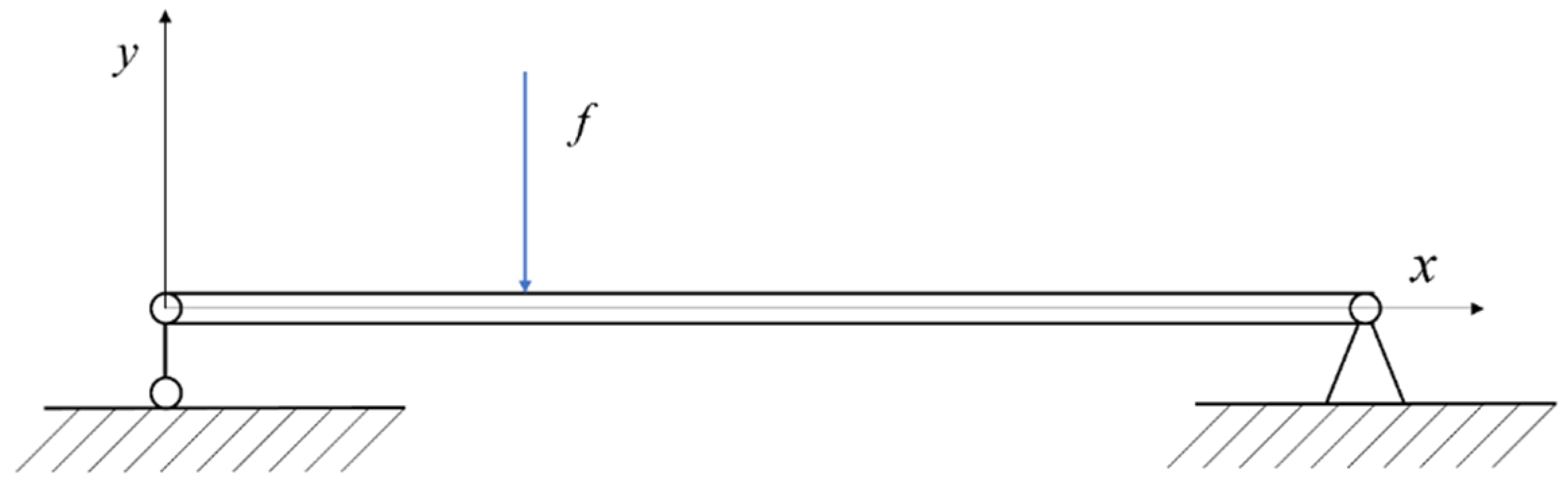
The simply supported beam has a length of $L=0.7 \mathrm{m}$, a cross-section of 0.04 m × 0.008 m, an elastic modulus of $E=2.1\times {10}^{11}$ N/m², a mass density of $\rho =7800$ kg/m³, and a Poisson’s ratio of 0.3. The system damping is proportional, and the damping ratio for each order is set at 0.02. The left end of the beam is designated as the position origin, and a load is applied at $x_f=0.4051$ m. This model is depicted in Figure 1. Acceleration response measurement points are arranged at distances of 0.14 m, 0.28 m, 0.42 m, and 0.56 m from the origin, with the sampling frequency set to 10,000 Hz. The Wilson-θ method is employed to calculate the acceleration response, simulating the acceleration response of the measurement points, with NTM and VSRPM used, respectively, for load positioning and identification.

4.1. Case 1: Impact Load without Noise

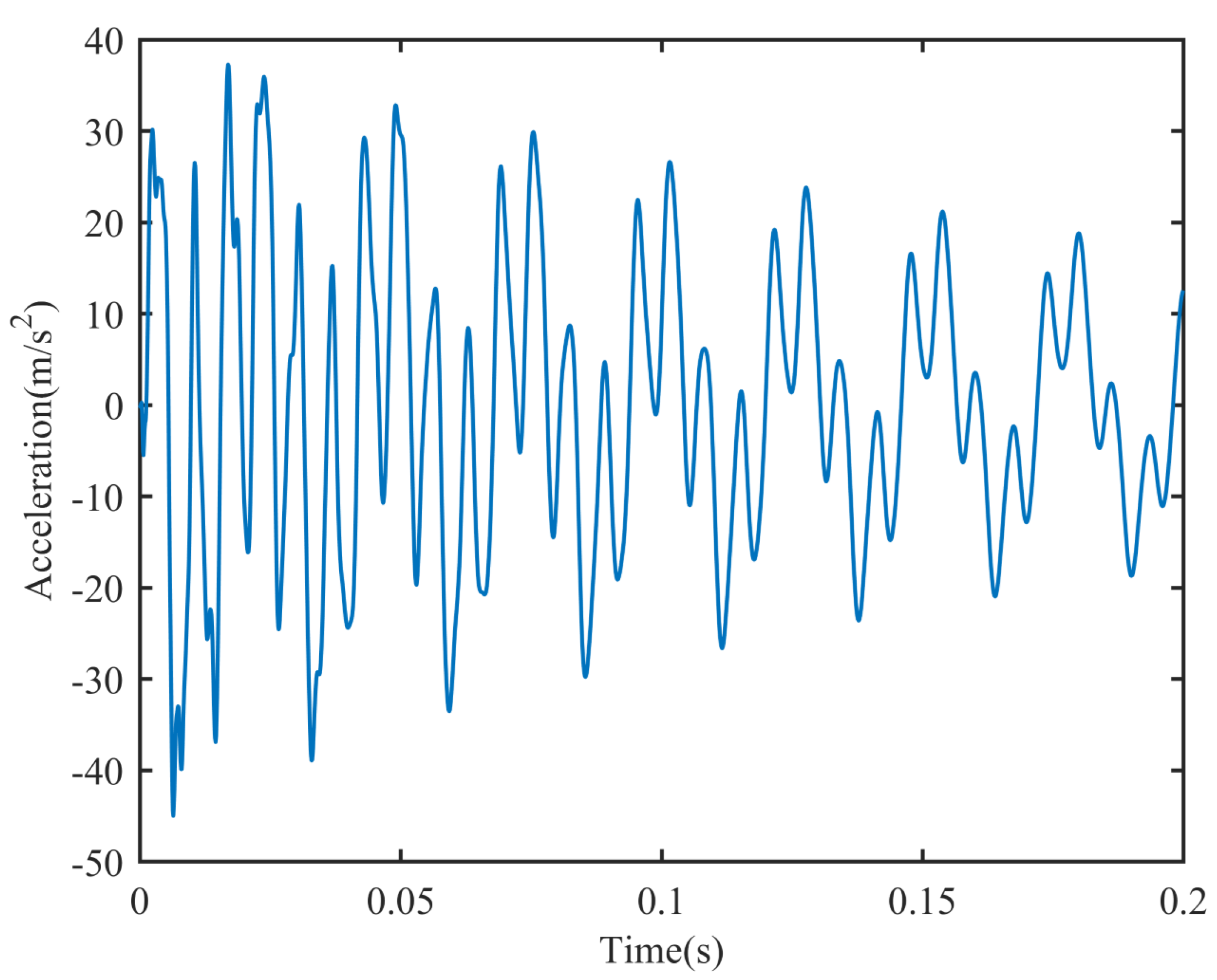
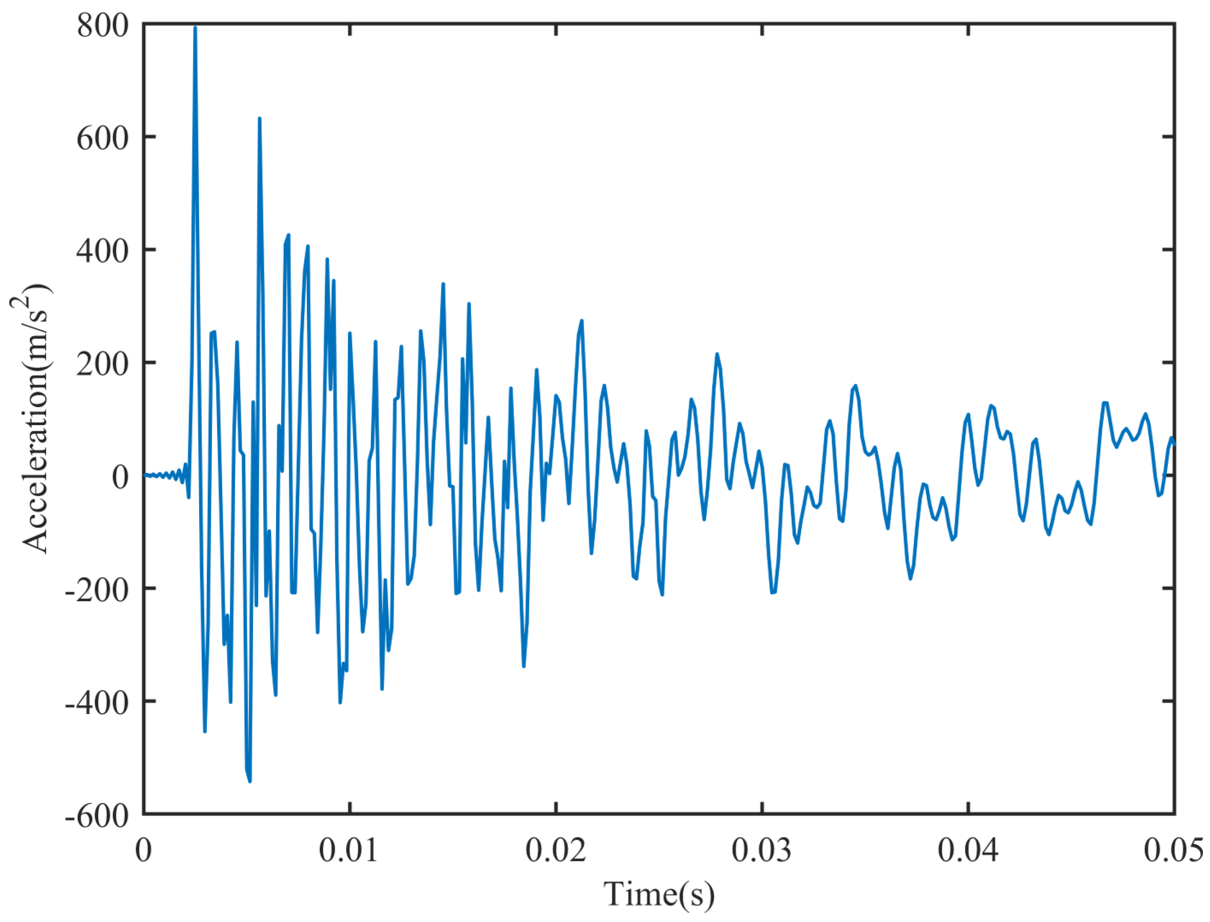
A half sine wave is used to simulate the impact load, with a load amplitude of 50 N and a load action time of 0.002 s. The acceleration response is resampled at a sampling frequency of 5000 Hz, followed by the use of the acceleration response of the VSRPM and NTM measurement points for load positioning and source finding.

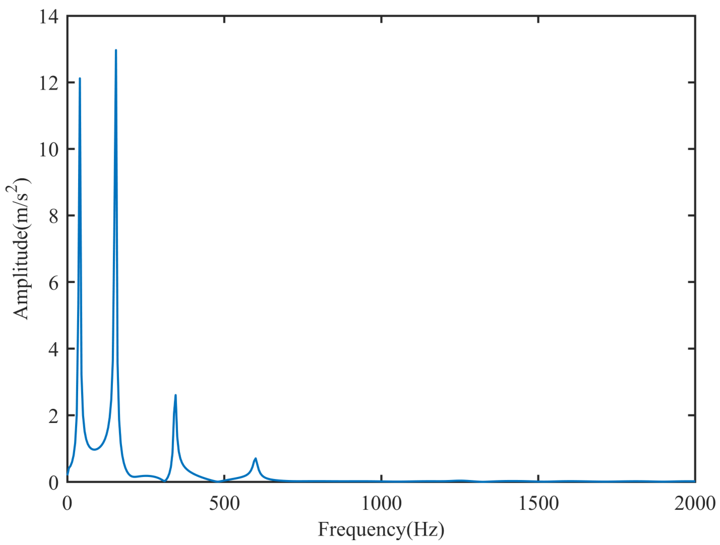
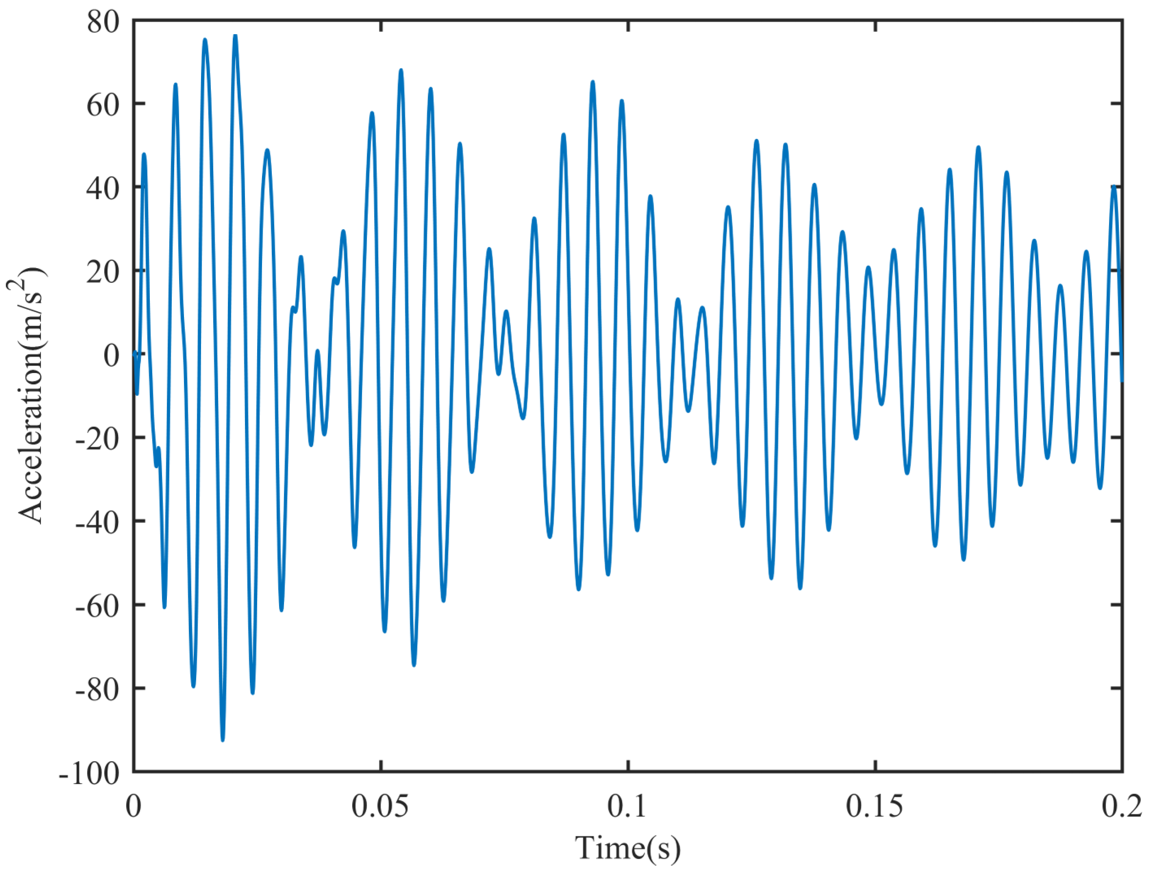
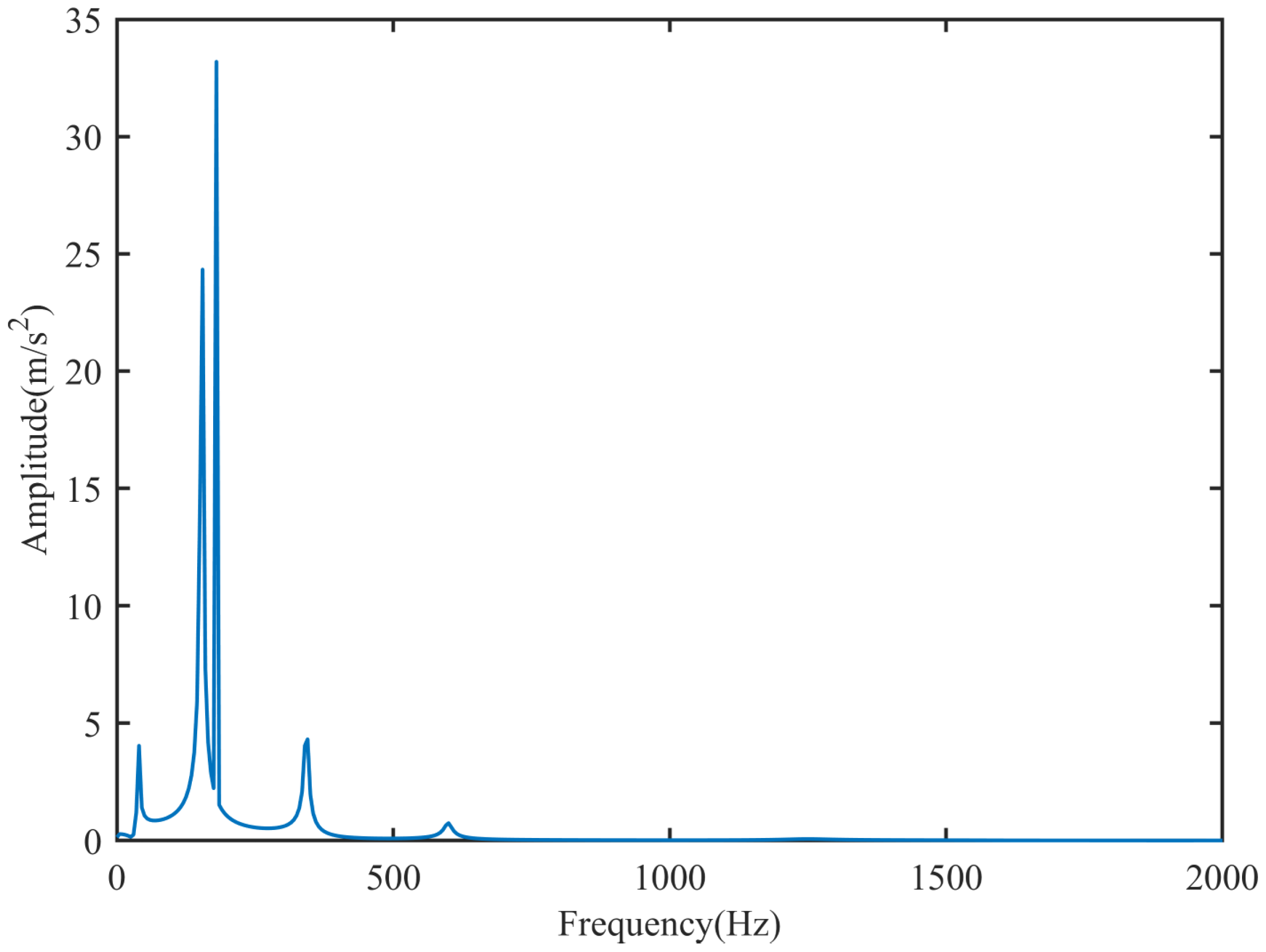
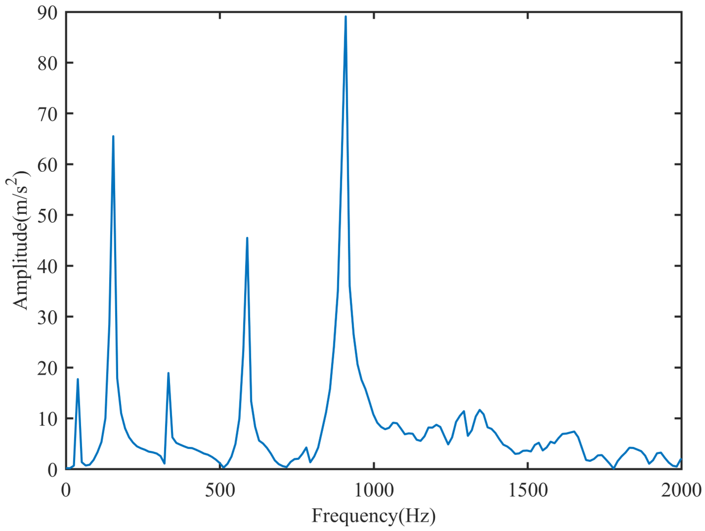
Figure 2 depicts the time-domain acceleration response of measurement point 1. Upon performing an FFT transformation, the frequency-domain acceleration response shown in Figure 3 is obtained. As observed from Figure 3, the first four modal orders dominate. To improve the identification accuracy, at least four measurement points should be selected. This confirms that the arrangement of four measurement points made previously is reasonable.

The computer utilized is the Huawei MateBook 2020 model, equipped with an Intel Core i7 processor. The step size for VSRPM source finding is established at 0.0001 m, and the initial value for NTM iteration is set at 0.2 m, eliminating the need to set the iteration step size.

This paper introduces two methods for evaluating identification effects, namely the Peak Relative Error Method (PREM) and the Signal-to-Noise Ratio (SNR). PREM represents the maximum peak error of the load identification result. A smaller PREM value indicates a better load identification result. SNR, the signal-to-noise ratio of the dynamic load identification result, describes the overall effect of dynamic load identification. A larger SNR value signifies a better effect of dynamic load identification.

$$\mathrm{PREM}=\frac{\left|\max p(t)-\max f(t)\right|}{\max f(t)}\times 100\%$$

(30)

$$\mathrm{SNR}=10{\log }_{10}\left[\frac{{\displaystyle \sum _{i=1}^b{\left(f(i)\right)}^2}}{{\displaystyle \sum _{i=1}^b{\left(f(i)-p(i)\right)}^2}}\right]$$

(31)

Here, $p(t)$ represents the identified load, $f(t)$ represents the real load loaded by the system, and $b$ represents the number of time steps.

Both VSRPM and NTM select the first two modes to determine the load position.

As observed from

Table 1. Comparison of payload identification results between VSEPM and NTM.

	${\mathit{x}}_{\mathit{f}}^{*}$ (m)	$\mathit{\Delta }{\mathit{x}}_{\mathit{f}}^{*}$ (m)	Time Taken (s)	PREM (%)	SNR
VSEPM	0.4054	0.0003	0.0311	0.078	56.62
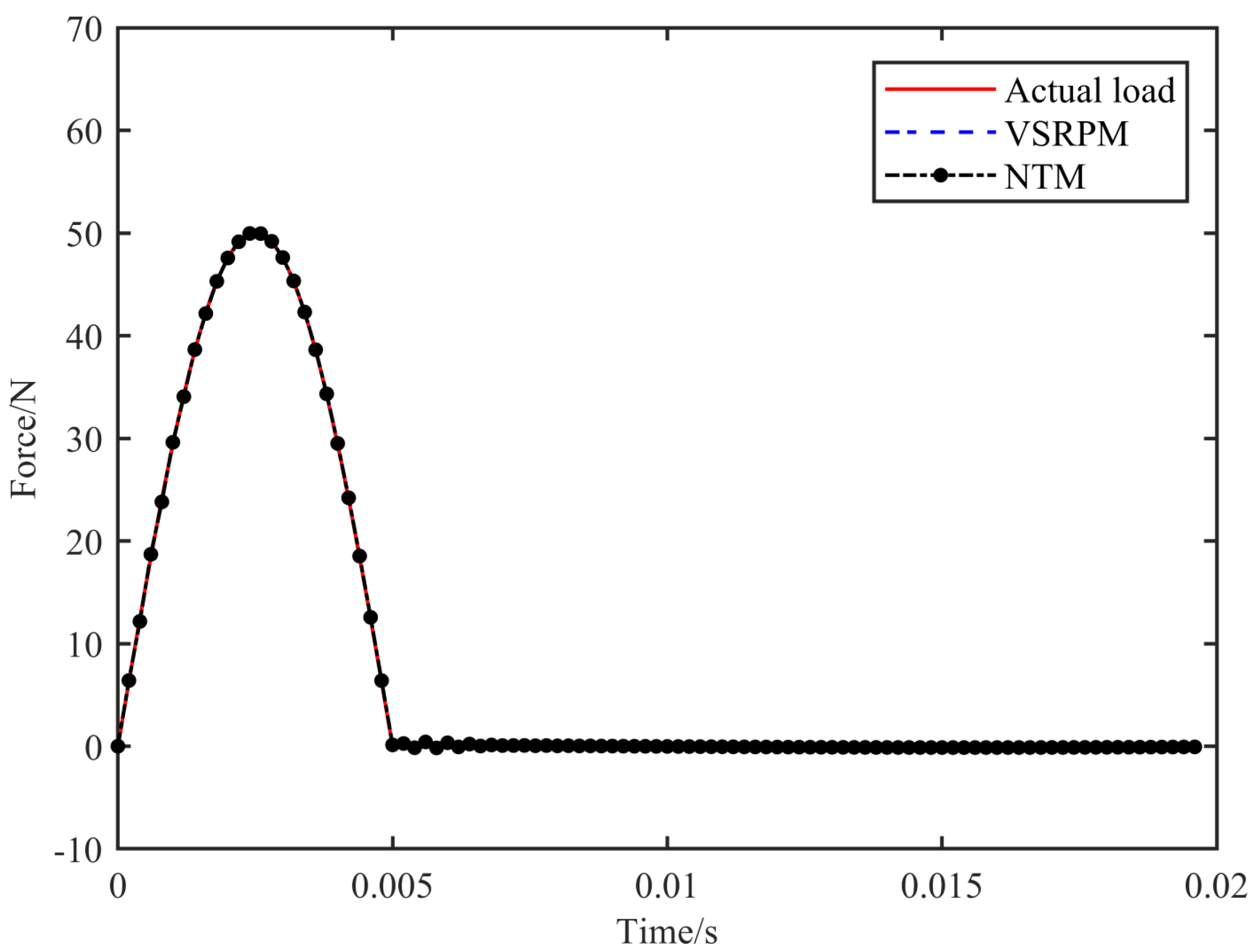
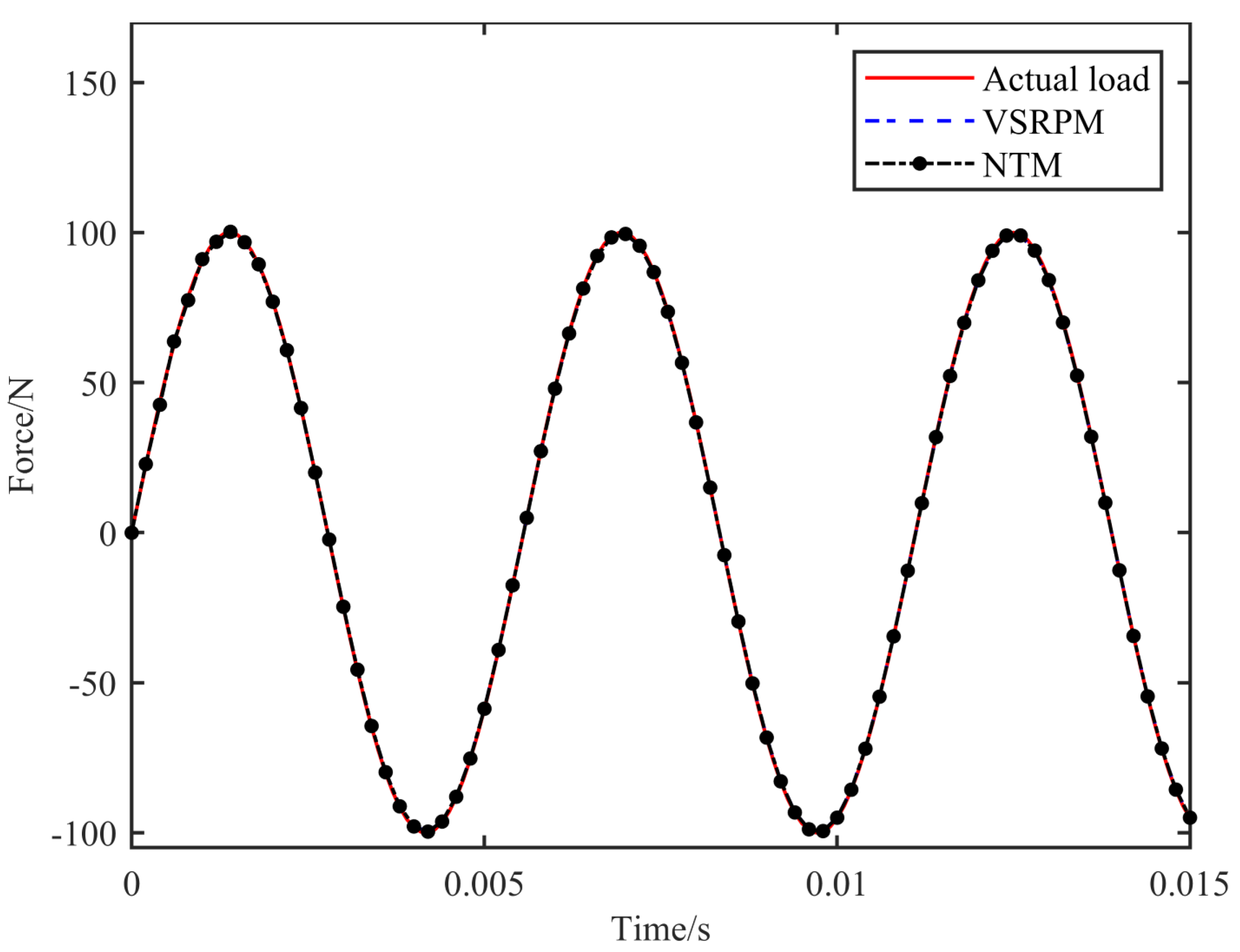
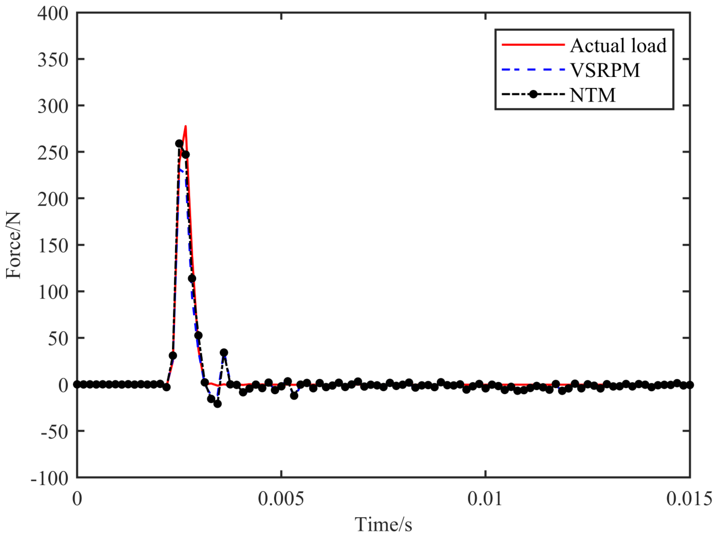
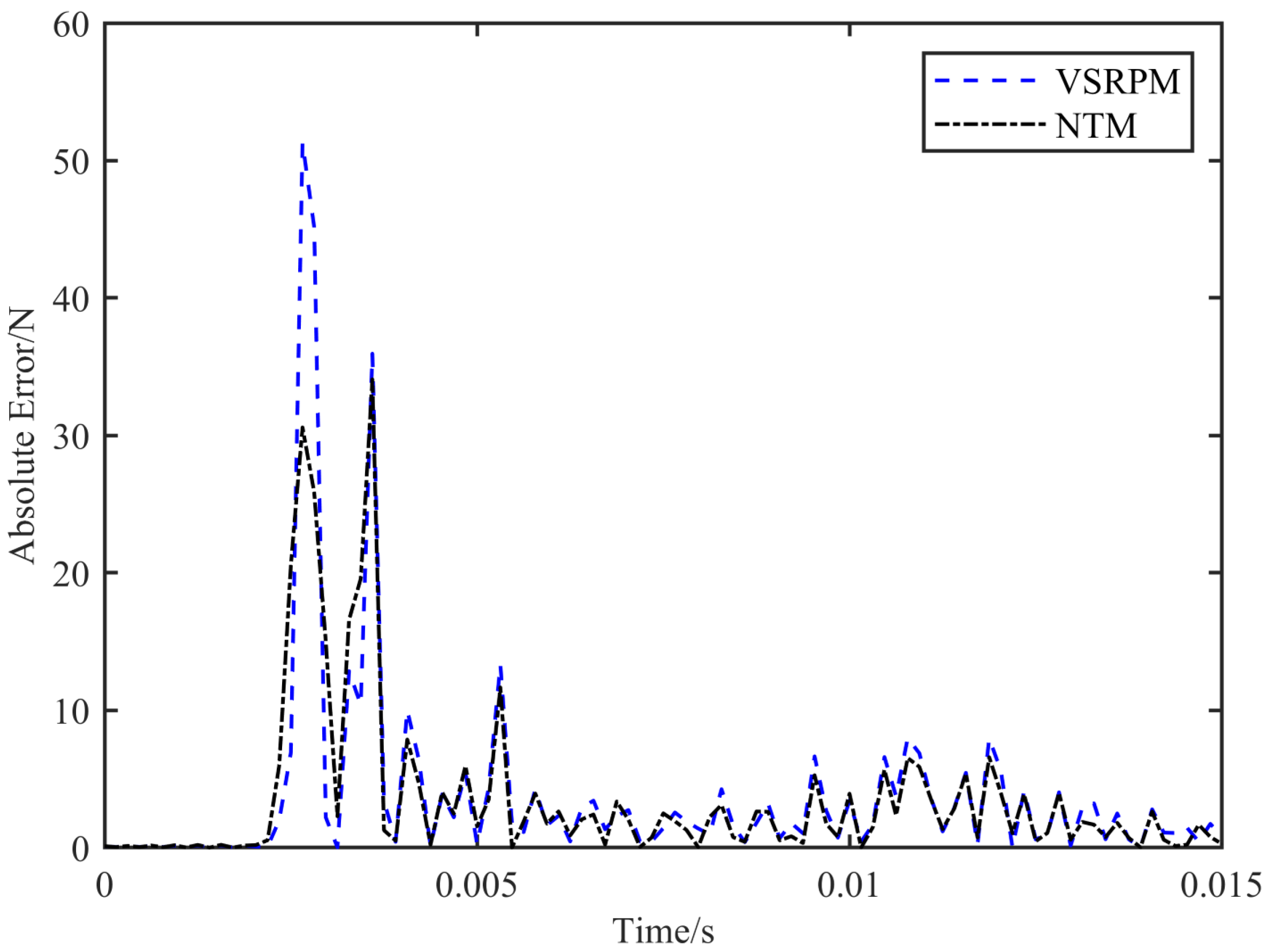
NTM	0.4052	0.0001	0.0043	0.052	57.88

, NTM identifies the load position with greater precision than VSRPM and takes less time. The load positioning process of VSRPM necessitates 0.0311 s, whereas that of NTM requires 0.0043 s. The computational efficiency of NTM has been enhanced by 86.17%. Upon determining the load position, the process of NTM and VSRPM recognizing the load schedule remains identical. Combining Figure 4 and Figure 5, it is evident that both NTM and VSRPM can accurately identify the schedule of the impact load, and the efficacy of NTM dynamic load recognition marginally surpasses that of VSRPM.

When the load position in NTM and VSRPM is artificially set to the actual load position of 0.04051 m, both methods yield a PREM value of 0.0443% and an SNR value of 57.93. This suggests that the discrepancies in the errors of the two algorithms are attributable to the deviation in the load position.

As observed from

Table 2. The relationship between the number of measuring points and the dynamic load identification results.

Number of Measuring Points	Measuring Point Coordinates (m)	NTM			VSRPM
		${\mathit{x}}_{\mathit{f}}^{*}\left(\mathbf{m}\right)$	Time Taken (s)	SNR	${\mathit{x}}_{\mathit{f}}^{*}\left(\mathbf{m}\right)$	Time Taken (s)	SNR
2	[0.3, 0.8]*L	0.4076	0.0041	30.71	0.4037	0.0288	30.53
3	[0.3, 0.6, 0.9]*L	0.4067	0.0037	39.04	0.4072	0.0296	39.01
4	[0.2, 0.4, 0.6, 0.8]*L	0.4052	0.0043	57.88	0.4054	0.0311	56.62
5	[0.1, 0.3, 0.5, 0.7, 0.9]*L	0.4051	0.0033	62.46	0.4051	0.0306	62.46
7	[0.1, 0.3, 0.4, 0.5, 0.6, 0.7, 0.8]*L	0.4051	0.0048	71.93	0.4051	0.0333	71.93
9	[0.1, 0.2, 0.3, 0.4, 0.5, 0.6, 0.7, 0.8, 0.9]*L	0.4051	0.0037	97.68	0.4051	0.0366	97.68

“*” in Table 2 indicates vector multiplication. For example, [0.3, 0.8]*L indicates that the measuring point position is [0.21, 0.56].

, an increase in the number of measurement points leads to more accurate load positioning of NTM and VSRPM and enhances the accuracy of the identified load time course. Given the same number of measurement points, the recognition accuracy of NTM slightly surpasses that of VSRPM.

In Table 1. Comparison of payload identification results between VSEPM and NTM, $\Delta x_f^{*}$ represents the absolute error of load positioning.

$$\Delta x_f^{*}=\left|x_f^{*}-x_f\right|$$

(32)

Here, $x_f^{*}$ represents the recognized load position and $x_f$ represents the actual load position.

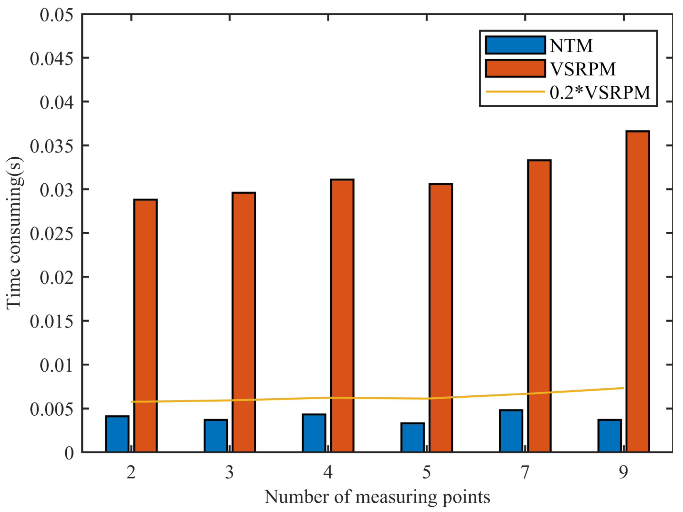
Figure 6 intuitively illustrates the comparison of the time consumption of NTM and VSRPM under varying numbers of measurement points. The specific arrangement of the measurement points aligns with Table 2. Here, “0.2VRSPM” denotes 20% of the time taken by VSRPM. The time consumption of NTM is significantly less than that of VSRPM, and all are below 0.2VRSPM. This implies that compared with VSRPM, the efficiency of NTM has been enhanced by more than 80%.

4.2. Case 2: Harmonic Load without Noise

Similarly, the sine load $F(t)=100\sin (360\pi t)$ N is loaded with a sampling frequency of 5000 Hz. The load loading position and measuring point arrangement are the same as in Case 1.

Figure 7 depicts the time-domain acceleration response of measurement point 1. The position coordinate of measuring point 1 is 0.14 m. Figure 8 represents the frequency-domain acceleration response of measurement point 1. The figure exhibits five peaks. The third peak from left to right corresponds to a load frequency of 180 Hz, while the other four peaks suggest that the first four modes dominate, thus making four measurement points reasonable.

Both VSRPM and NTM select the first two modes to determine the load position.

As can be seen from

Table 3. Comparison of payload identification results between VSEPM and NTM.

	${\mathit{x}}_{\mathit{f}}^{*}\left(\mathbf{m}\right)$	$\mathit{\Delta }{\mathit{x}}_{\mathit{f}}^{*}$ (m)	Time Taken (s)	PREM (%)	SNR
VSEPM	0.4048	0.0003	0.0385	0.22	66.12
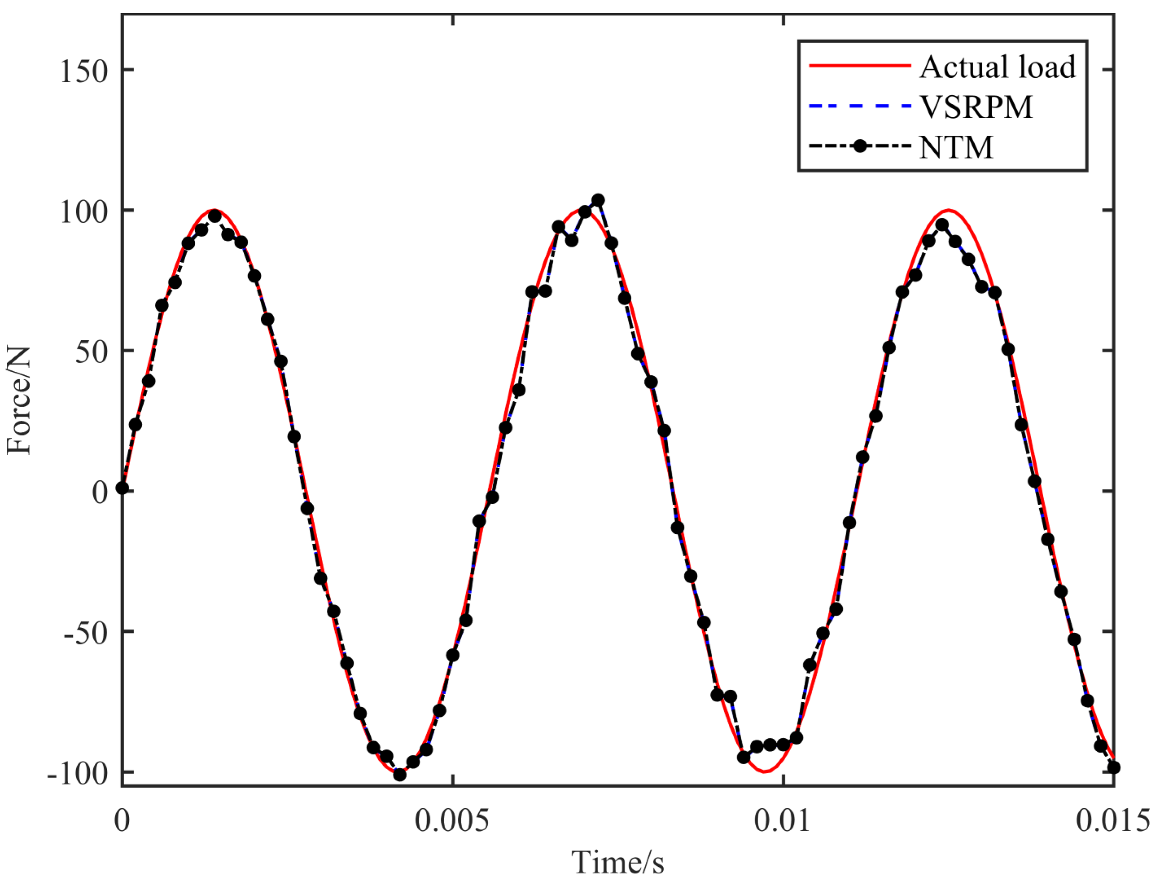
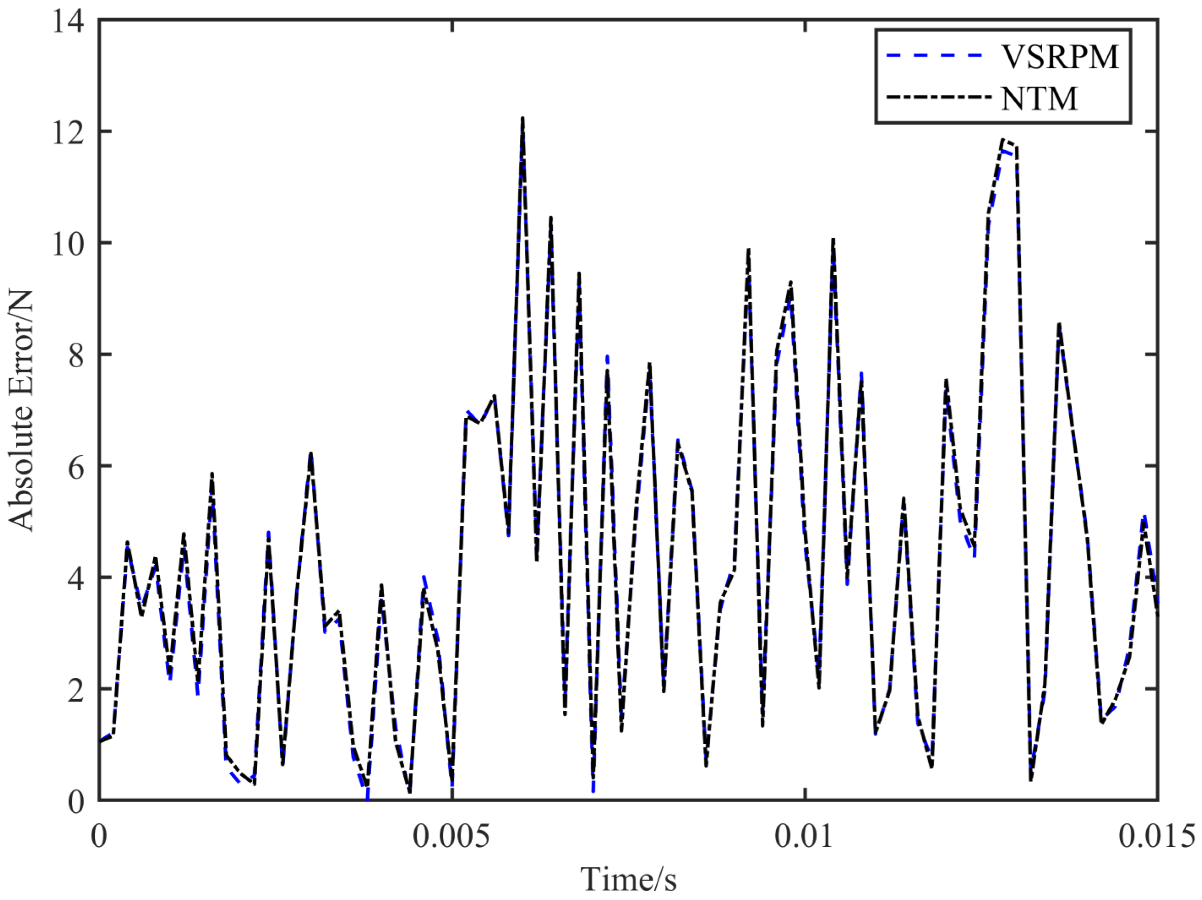
NTM	0.4050	0.0001	0.0070	0.19	67.04

, the position recognition accuracy of NTM is slightly higher than that of VSRPM. In terms of time consumption, VSRPM takes 0.0385 s, whereas NTM takes 0.0070 s. This results in a time saving of 81% and a significant improvement in calculation efficiency. From the perspective of the time course of load recognition, the PREM value of NTM is 0.19% and the SNR value is 67.04, while the PREM value of VSRPM is 0.22% and the SNR value is 66.12. This indicates that the accuracy of the load time course recognized by NTM surpasses that of VSRPM. Figure 9 and Figure 10 also prove that NTM is more accurate. Therefore, it can be concluded that NTM is not only suitable for the recognition of sine loads but also surpasses VSRPM in terms of efficiency and accuracy.

4.3. Case 3: Random Dynamic Load Identification

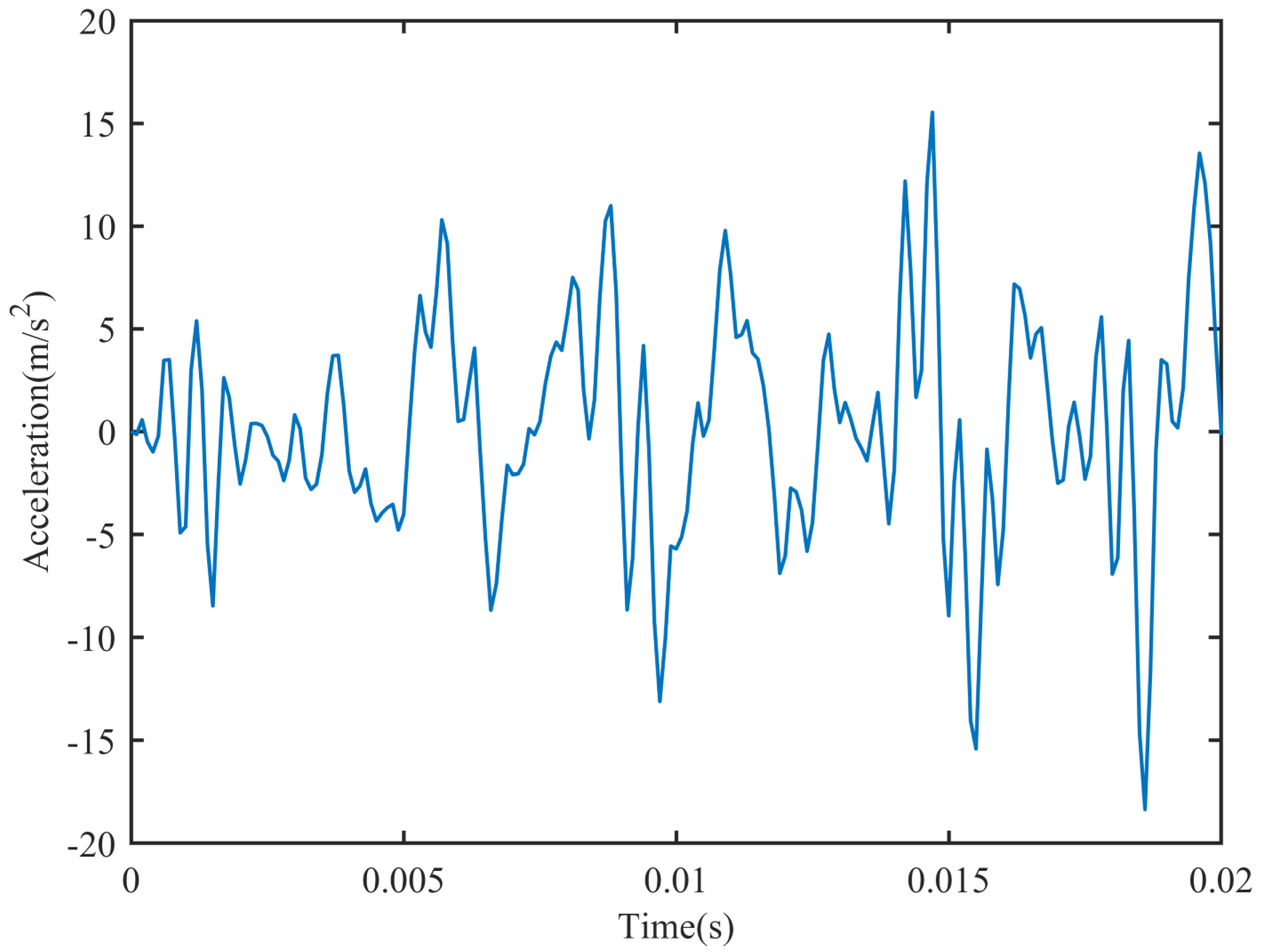
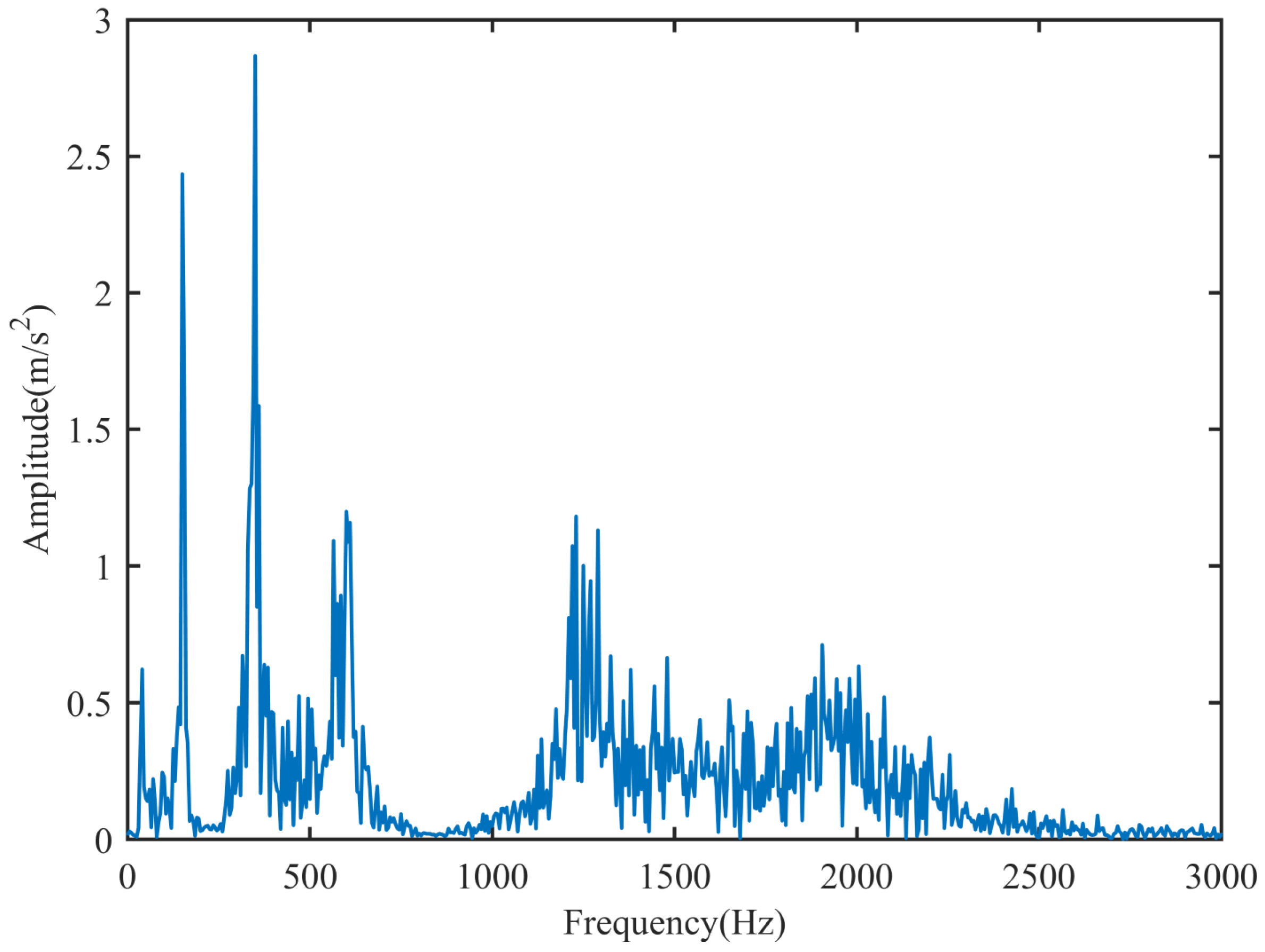
The load from Case 1 is altered to a random dynamic load with an amplitude ranging from −5 N to 5 N, and the loading duration is set at 0.02 s. The position of the load is kept unchanged. Figure 11 and Figure 12 depict the acceleration response of measurement point 1. As observed from Figure 12, the frequency band excited by the random load is broader, necessitating an increase in the number of measurement points to ensure that the accurate modal load is obtained. Therefore, eight measurement points are arranged to obtain the acceleration response. The positions of the measurement points are, respectively, [0.2,0.3,0.4,0.5,0.6,0.7,0.8,0.9]L. The sampling frequency of the acceleration response is established at 10,000 Hz.

Both VSRPM and NTM select the first two modes to determine the load position.

As observed in

Table 4. Comparison of payload identification results between VSEPM and NTM.

	${\mathit{x}}_{\mathit{f}}^{*}$ (m)	$\mathit{\Delta }{\mathit{x}}_{\mathit{f}}^{*}$ (m)	Time Taken (s)	PREM (%)	SNR
VSRPM	0.4049	0.0002	0.0393	0.09	98.44
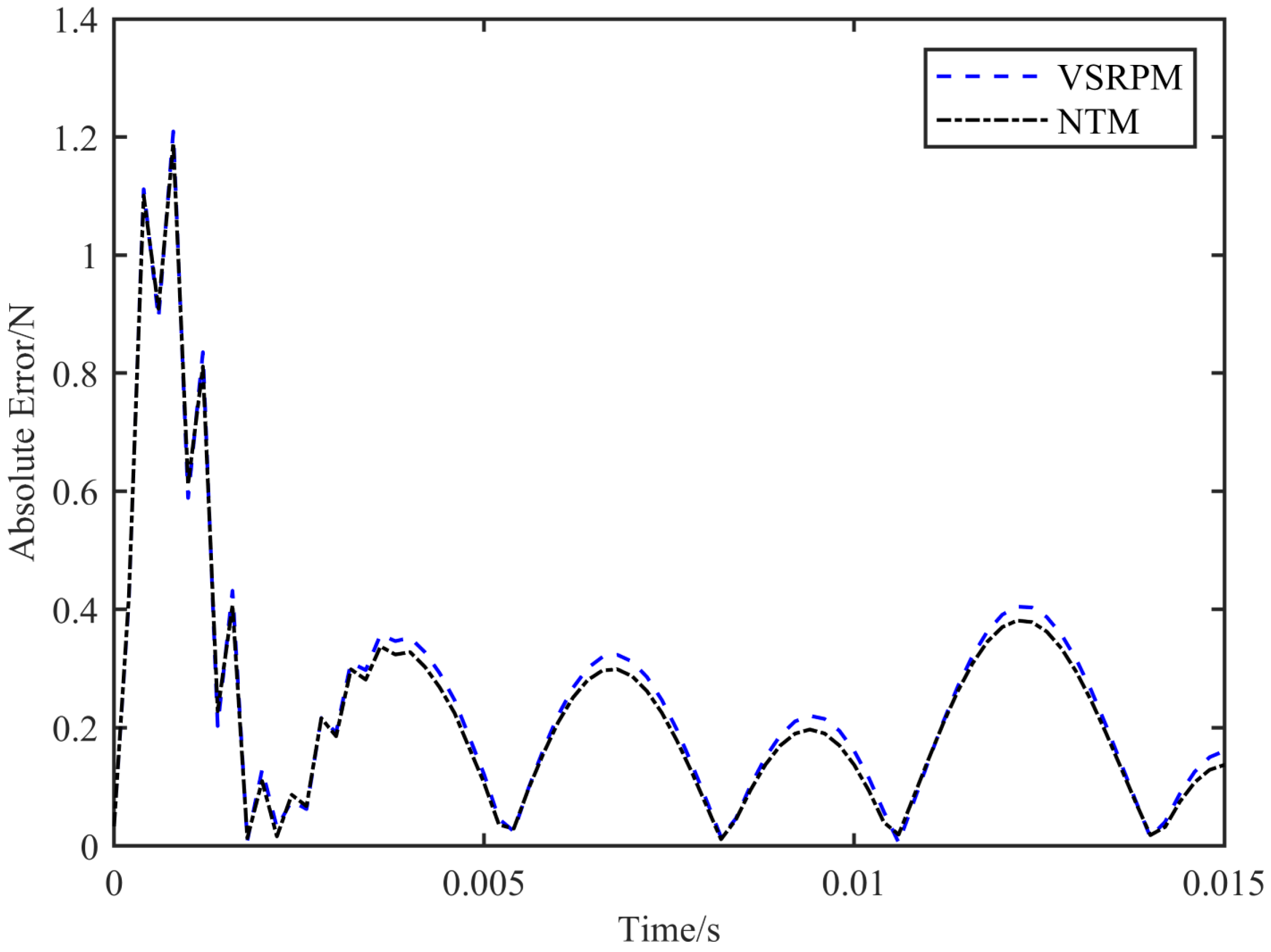
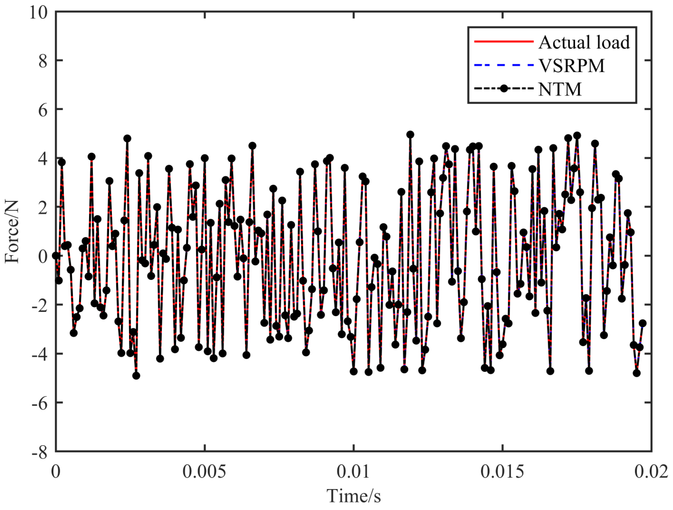
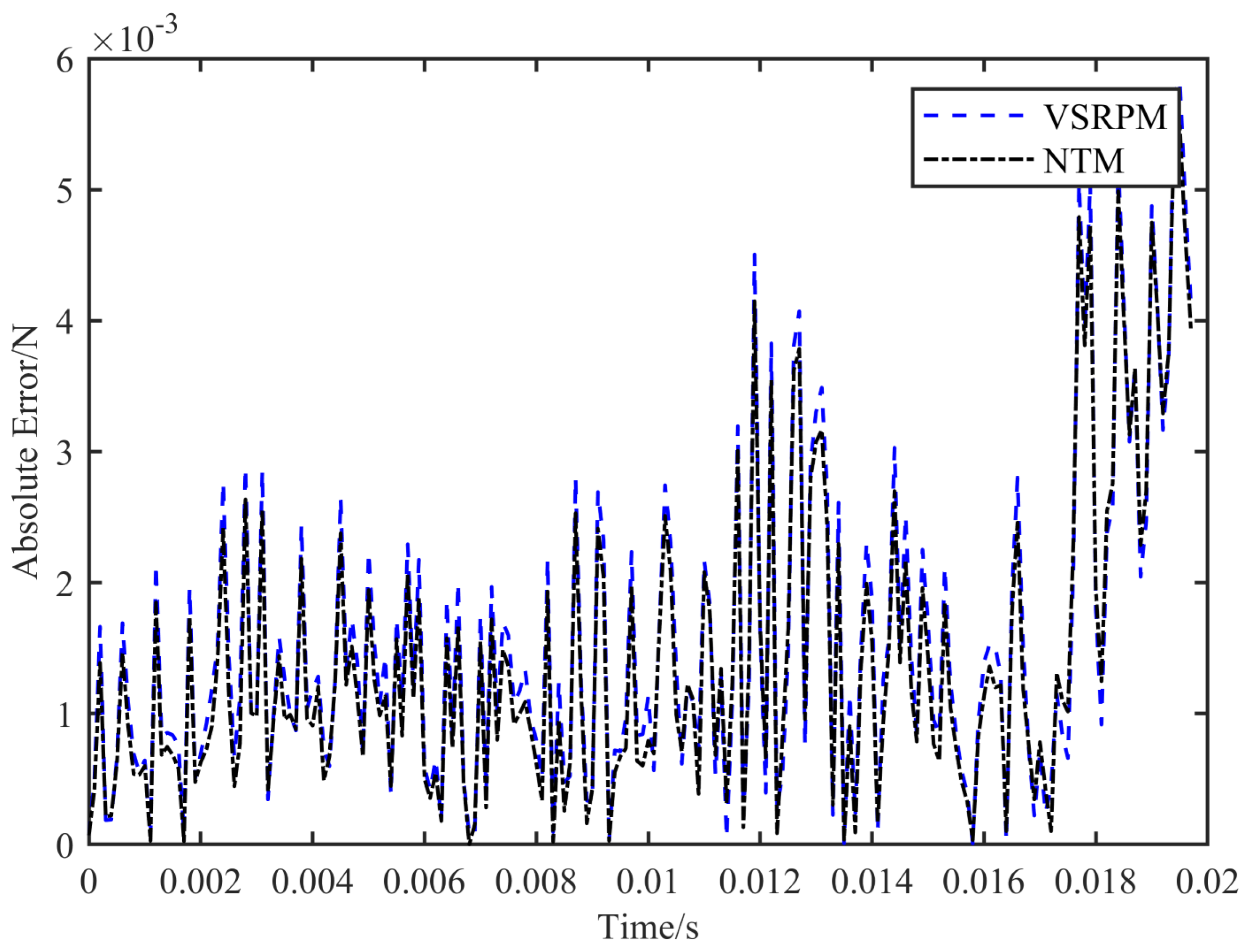
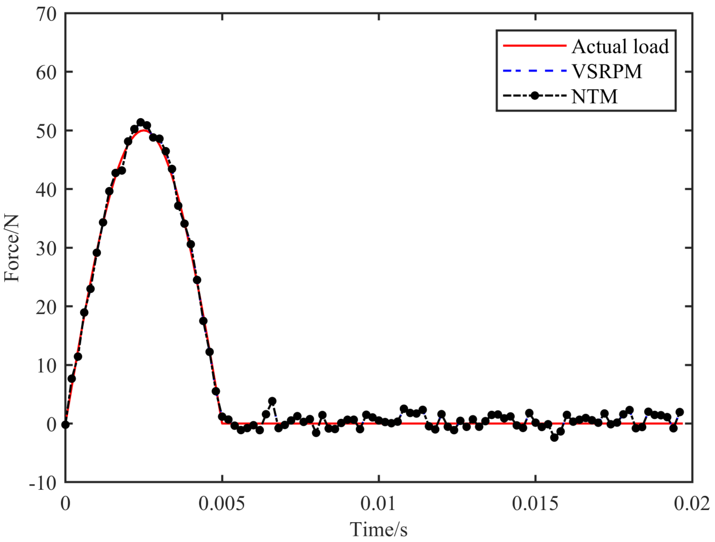
NTM	0.4050	0.0001	0.0076	0.08	98.80

, the load position identified by NTM is more precise than that identified by VSRPM, and the time taken constitutes only 19.34% of that of VSRPM. Combining Figure 13 and Figure 14, the load time course identified by NTM is closer to the actual load than that identified by VSRPM. Therefore, it can be inferred that NTM applies to random loads, and it holds advantages in terms of efficiency and precision.

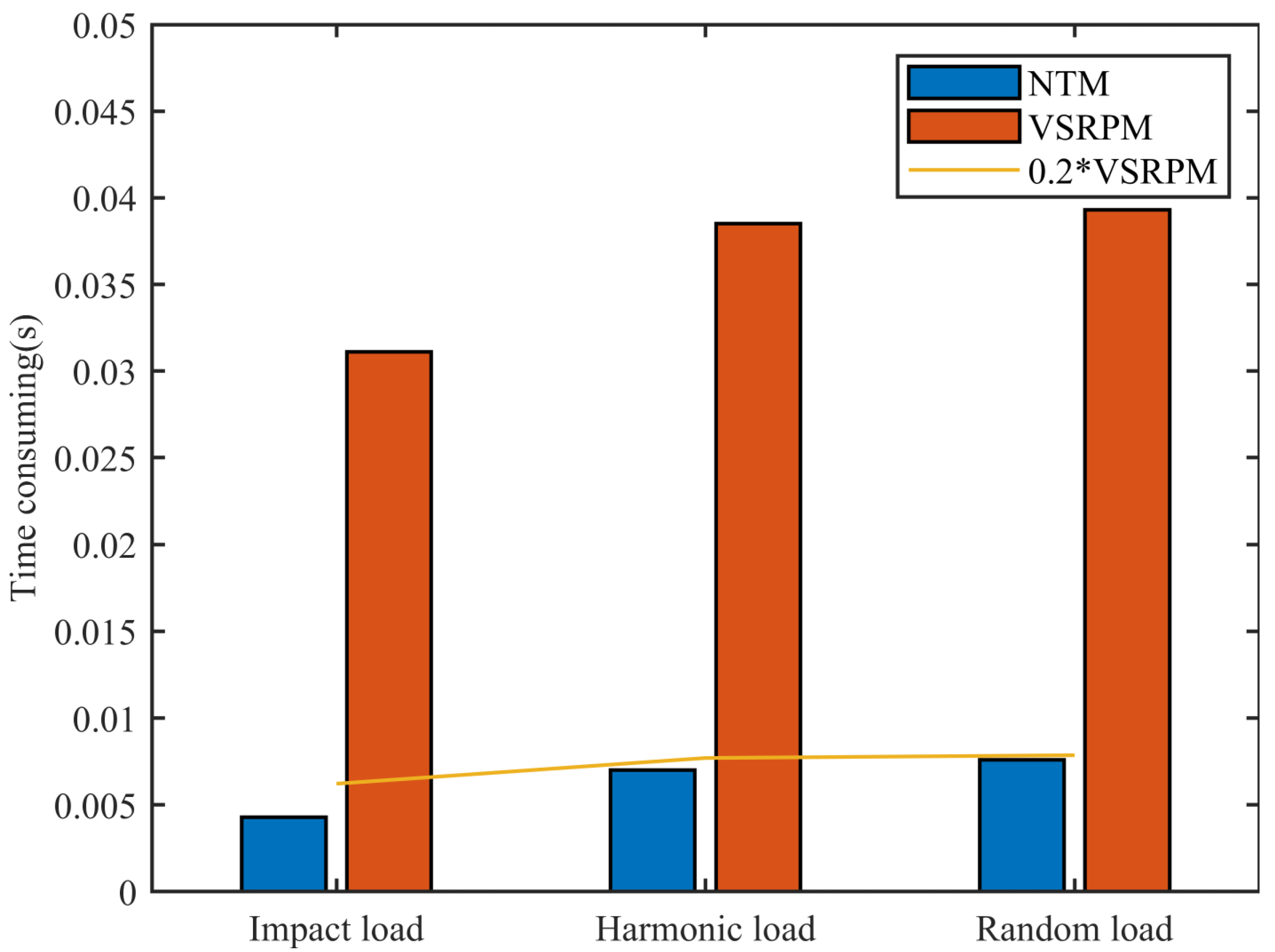
Figure 15 illustrates the time taken by NTM and VSRPM when positioning varying types of loads. From the figure, it can be inferred that irrespective of whether it is an impact load, a sinusoidal load, or a random load, the time taken by NTM for load positioning is less than 20% of that of VSRPM. The speed of NTM is once again demonstrated.

4.4. Case 4: Noisy Dynamic Load Identification

Gaussian white noise with SNR = 30 db, 25 db, and 20 db is incorporated into the acceleration responses of Case 1 and Case 2, respectively, to emulate the recognition effect under actual conditions and validate the efficiency and accuracy of NTM.

Figure 16 and Figure 17 illustrate that under the condition of acceleration response SNR = 25 db, NTM can also accurately identify the position and time course of the impact load. Figure 18 and Figure 19 illustrate that under the condition of acceleration response SNR = 25 db, NTM can accurately identify the position and time course of the sine load. Please refer to

Table 5. Comparison of load identification results between NTM and VSRPM under noisy acceleration response.

Load Type	SNR of Acceleration Response	$\mathit{\Delta }{\mathit{x}}_{\mathit{f}}^{*}/\mathbf{m}$		Time Taken/s			SNR of Identifying Dynamic Loads
		NTM	VSRPM	NTM	VSRPM	$\mathit{\epsilon }$	NTM	VSRPM
Impact load	30 db	0.0001	0.0004	0.0042	0.0320	13.13%	53.38	53.32
	25 db	0.0002	0.0009	0.0040	0.0337	11.87%	42.66.	42.47
	20 db	0.0004	0.0012	0.0057	0.0312	18.27%	31.17	31.14
Sinusoidal load	30 db	0.0001	0.0002	0.0068	0.0347	19.59%	54.25	53.83
	25 db	0.0003	0.0009	0.0054	0.0368	14.67%	43.20	42.41
	20 db	0.0008	0.0013	0.0069	0.0395	17.47%	30.98	30.66

for specific data on load positioning and identification.

Table 5 documents the comparison results of NTM and VSRPM in terms of position recognition accuracy, position recognition efficiency, and load time course recognition accuracy under varying signal-to-noise ratio acceleration response conditions. Overall, a larger signal-to-noise ratio of the acceleration response leads to more accurate load positioning and a higher conformity of the recognized load time course to the actual load time course. NTM can effectively identify the load position and time course when the SNR of the acceleration response is greater than or equal to 20 db. Whether in terms of computational efficiency or accuracy, it surpasses VSRPM. Specifically, the time taken by NTM in the process of load positioning constitutes less than 20% of that taken by VSRPM. This indicates that NTM significantly enhances the efficiency of load positioning and is a remarkably fast algorithm.

In Table 5, $\epsilon$ represents the ratio of the time taken in the load positioning process of NTM to VSRPM.

$$\epsilon =\frac{T_{NGM}}{T_{VSRPM}}\times 100\%$$

(33)

Here, $T_{NGM}$ represents the time taken in the process of load positioning by NTM, and $T_{VSRPM}$ represents the time taken in the process of load positioning by VSRPM.

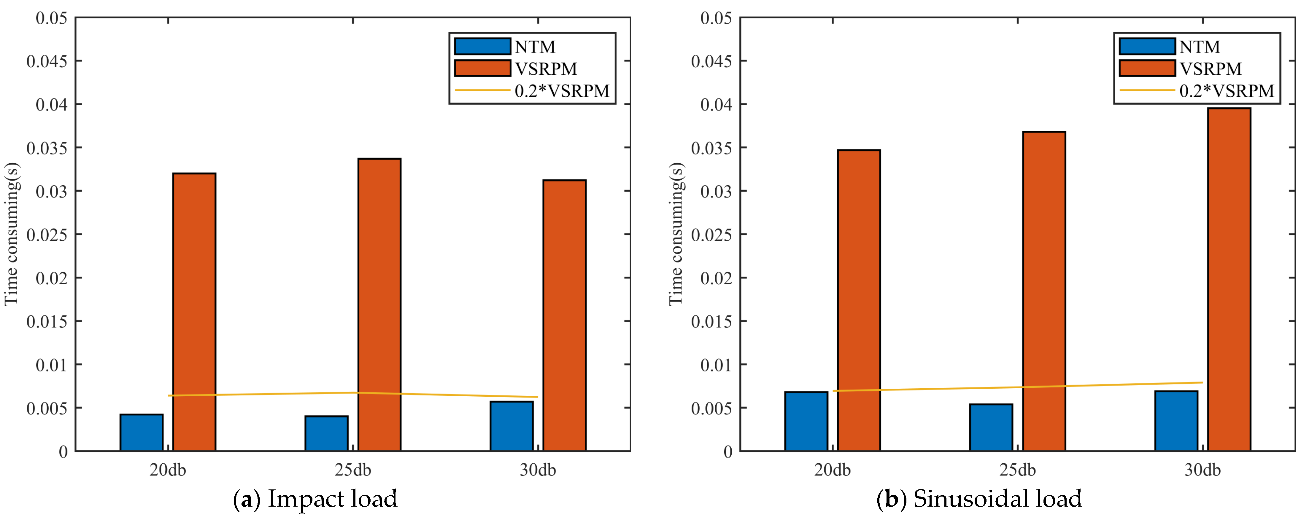
Figure 20 clearly shows the time taken by NTM and VSRPM in positioning loads under the condition of acceleration response with noise. From the figure, it is evident that the time taken by NTM is much less than that of VSRPM, resulting in a saving of at least 80% of the calculation time. This further demonstrates that NTM is an efficient method for load positioning and recognition.

5. Experimental Verification

A simply supported beam experiment was designed to verify the effectiveness of NTM. After the modal test, the basic parameters of the beam were determined. The length of the beam was L = 0.7 m, the thickness was 0.008 m, and the width was 0.04 m. The beam’s cross-section was rectangular, and the cross-sectional moment of inertia was I = 1.707 × 10⁻⁹ m⁴. The elastic modulus of the beam was = 2.05 × 10¹¹ N/m², the mass density was ρ = 7800 kg/m³, and Poisson’s ratio was 0.3. The system damping exhibited proportional damping.

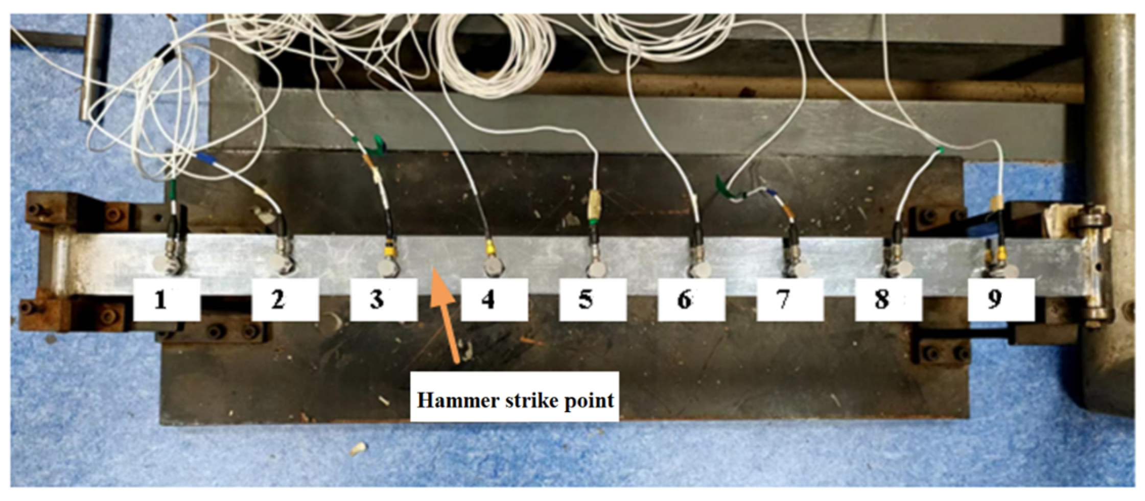
The left endpoint of the beam was designated as the position origin, and the hammering point was located at x = 0.21 m. Acceleration response sensors were arranged at distances of 0.07 m, 0.14 m, 0.21 m, 0.28 m, 0.35 m, 0.42 m, 0.49 m, 0.56 m, and 0.63 m from the origin, respectively, with the sampling frequency set to 6400 Hz. Figure 21 shows the beam used in the experiment and the specific distribution of the nine measuring points.

By observing

Table 6. Comparison between experimental model and simulation model.

Modal Order	Experimental Model Natural Frequency/Hz	Simulation Model Natural Frequency/Hz	Damping Ratio
1	38.85	37.85	0.002
2	153.46	151.81	0.007
3	341.80	341.58	0.005
4	601.48	607.26	0.003
5	933.11	948.84	0.040
6	1320.1	1366.23	0.051

, it can be seen that the first six inherent frequencies of the simulation model deviated by less than 5% from the experimental model, thus rendering the simulation model usable.

Figure 22 depicts the time-domain response of measurement point 3. After FFT transformation, the frequency-domain response depicted in Figure 23 was obtained. To ensure recognition accuracy, the acceleration response of nine measurement points was utilized to identify the load.

Both VSRPM and NTM select the first two modes to determine the load position.

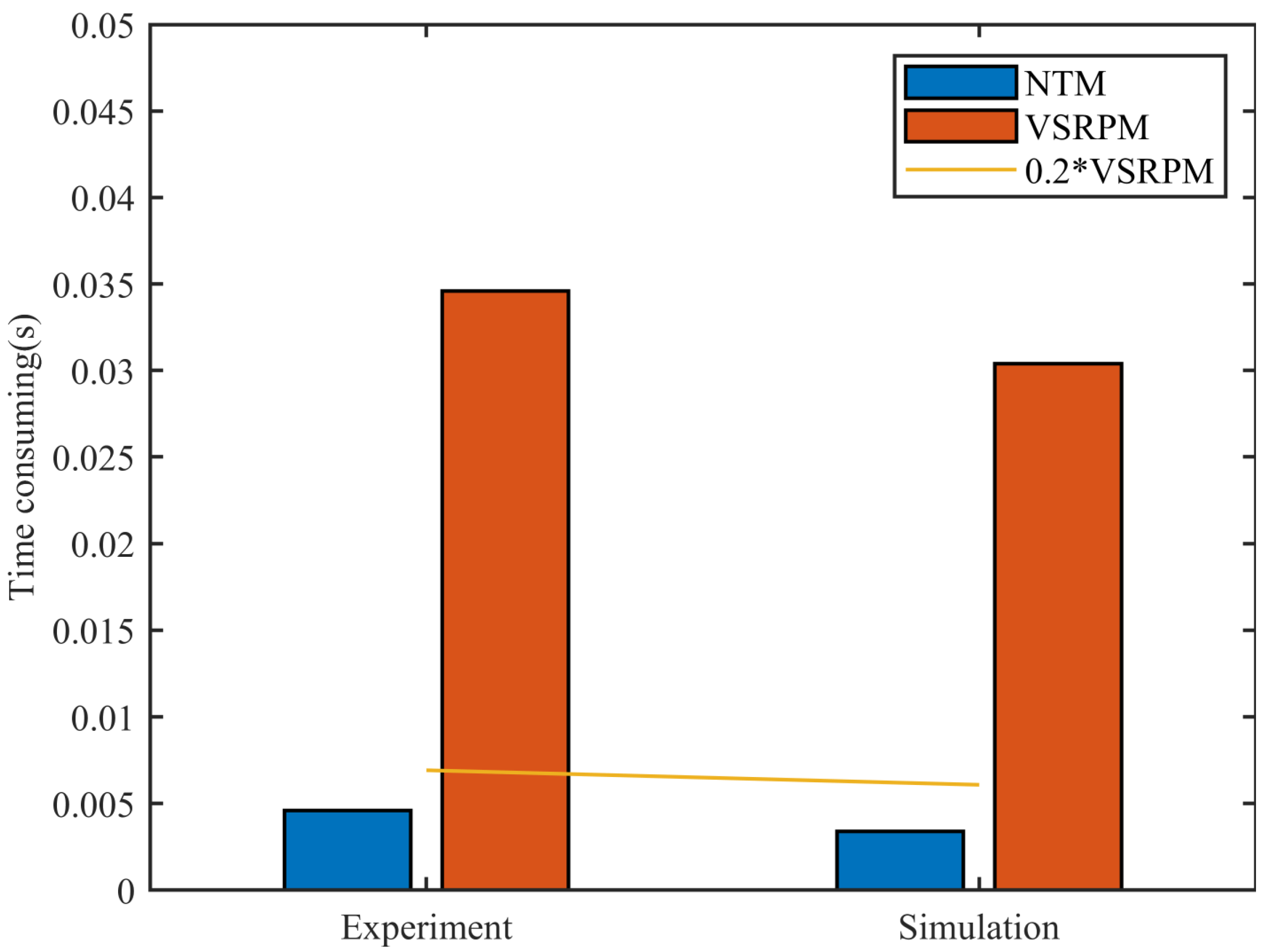
In

Table 7. Comparison of load identification results between NTM and VSRPM.

		${\mathit{x}}_{\mathit{f}}^{*}/\mathbf{m}$	$\mathit{\Delta }{\mathit{x}}_{\mathit{f}}^{*}/\mathbf{m}$	Time Taken/s	PREM/%	SNR
Experiment	VSRPM	0.2027	0.0073	0.0346	16.65	29.15
	NTM	0.2128	0.0028	0.0046	6.73	35.05
Simulation	VSRPM	0.2111	0.0011	0.0304	2.1612	37.41
	NTM	0.2096	0.0004	0.0034	0.0756	72.68

, “Experiment” refers to the process of load positioning and recognition using the acceleration response measured directly from the experiment. On the other hand, “Simulation” refers to the process where the measured hammer load was inputted into the simulation model to calculate the acceleration response, and then the simulated acceleration response was used for load positioning and recognition. Figure 22, Figure 23, Figure 24 and Figure 25 all contain data from the “Experiment”.

From Table 7, we can clearly observe the data comparison from the “Experiment”. When compared to VSRPM, the load position identified by NTM is more accurate and requires less time. The PREM value of NTM is lower than that of VSRPM, while the SNR value is higher than that of VSRPM. From Figure 24 and Figure 25, it is evident that the load time course identified by NTM is more closely aligned with the real load time course than that identified by VSRPM. This demonstrates that the results of load positioning and recognition produced by NTM are more effective than VSRPM.

Similarly, for “Simulation”, the load position and efficiency achieved by NTM are superior to VSRPM. Moreover, the recognition result of “Simulation” is more accurate than “Experiment”.

Figure 26 clearly compares the time consumption of the two algorithms under the conditions of “Experiment” and “Simulation”. From the figure, it is evident that regardless of whether it is under the condition of “Experiment” or “Simulation”, the efficiency of NTM in load positioning is 80% greater than that of VSPRM.

Whether they are compared with the Case 1 impact load simulation example or “Simulation”, the experimental results exhibit certain errors. The sources of the errors in the experimental results include errors caused by inaccurate model establishment, and measurement errors in acceleration response, among others. Despite the recognition result of the experiment containing certain errors, the result of load positioning and recognition is still satisfactory. In conclusion, the experimental results validate the effectiveness and speed of NTM.

6. Conclusions

This paper introduces a new NTM for dynamic load localization and identification. This method augments the number of measurement points to simultaneously recognize the load position and a suitable time course. Initially, the load position information and amplitude information are segregated, followed by the application of the Newton iteration method for load positioning; upon determining the load position, the load time course is resolved. Simulation examples and experiments demonstrate that this method boasts higher recognition accuracy than VSRPM and enhances computational efficiency by 80%. This indicates that NTM is an extremely valuable method for load positioning and recognition.

As this paper aims to propose a more efficient NTM method for dynamic load localization and identification, starting from a single-point concentrated load, this method can be explained more clearly. Theoretically, NTM can not only realize the positioning and recognition of single-point loads, but can also locate and recognize multi-point concentrated loads. It can even extend NTM to more complex structural systems. Therefore, future work will not only explore the extension of the NTM method to multi-point concentrated loads and discrete systems, but will also theoretically examine its applicability to plate structures and more complex three-dimensional model structures. This marks a key area of focus for our upcoming research endeavors, aiming to broaden the scope of NTM’s applicability. Additionally, addressing the dependency on the accurate solution of modal loads by introducing correction algorithms and regularization holds the potential for improving recognition accuracy.