Abstract
In recent years, the number of expected missions to the Moon has increased significantly. With limited terrestrial-based infrastructure to support this number of missions, as well as restricted visibility over intended mission areas, there is a need for space navigation system autonomy. Autonomous on-board navigation systems in the lunar environment have been the subject of study by a number of authors. Suggested systems include optical navigation, high-sensitivity Global Navigation Satellite System (GNSS) receivers, and navigation-linked formation flying. This paper studies the interoperable nature and fusion of proposed autonomous navigation systems that are independent of Earth infrastructure, given challenges in distance and visibility. This capability is critically important for safe and resilient mission architectures. The proposed elliptical frozen orbits of lunar navigation satellite systems will be of special interest, investigating the derivation of orbit determination by non-terrestrial sources utilizing celestial observations and inter-satellite links. Potential orbit determination performances around 100 m are demonstrated, highlighting the potential of the approach for future lunar navigation infrastructure.
AIArtificial Intelligence AOAAngle of Arrival DCMDirection-Cosine Matrix DOPDilution of Precision DRODirect Rectilinear Orbit EGMEarth Gravitational Model EKFExtended Kalman Filter ELFOElliptical Lunar Frozen Orbit ENUEast-North-Up FOVField of View GNSSGlobal Navigation Satellite System IERSInternational Earth Rotation and Reference Systems Service ISLInter-Satellite Link LCNSLunar Communication and Navigation Service LLOLow Lunar Orbit MEMean Earth NRHONear Rectilinear Halo Orbit
1. Introduction
The Moon is going to be very busy over the next decade [1,2,3]. In response, major international space players have proposed infrastructure to deliver communication and navigation services to satisfy increasing demand. These include LunaNet by NASA [4], Moonlight from ESA [5], and the Lunar Communication and Navigation Service (LCNS) from JAXA [6]. The performances required by users of this system are demanding, especially in terms of orbit determination, timing, data rates, and others. For LCNS, ten small satellites are being considered, where it is possible to maintain an orbit that meets positioning requirements with minimal orbit maintenance over 3 years [7].
A key performance criterion is an orbit determination accuracy of below 30 m [6], with each satellite transmitting a pseudo-like ranging signal to ground users, to deliver a surface positioning accuracy of 40 m. This performance target is feasible through the use of Earth-based tracking stations, where lunar pathfinder missions have delivered performances below 40 m in three dimensions [8]. However, the use of deep-space tracking networks is expensive, and they have infrequent visibility and a high user demand. They also create a strict dependence on distant Earth-based infrastructure.
As an LCNS by any space agency is a critical system for the successful delivery of an increasing number of future lunar missions, orbit determination must be more autonomous. However, meeting this performance is challenging with the current state of the art.
Various architectures have been evaluated to deliver this capability. A majority seek to utilize a high-sensitivity Global Navigation Satellite System (GNSS) receiver, relying on the side-lobes of Earth-based GNSS for operation [5,9]. However, performances are expected to reach only several 100 m with intermittent availability. A high-sensitivity antenna is also needed with high-pointing requirements to deliver these performances. No successful position fix has been announced yet from recently launched lunar-destined GNSS receivers [10].
Alternative architectures for lunar navigation include using the limb’s horizon. This will be demonstrated for satellites in cislunar space, such as Orion [11] and LUMIO [12]. Performances of these instruments alone might only reach up to 1–10 km. Other scenarios have also been studied [13,14,15,16], but most mission concepts have only treated cislunar operations or descent and landing.
Fused navigation for a lunar repeating orbit satellite has been considered in [17], where a combination of a horizon-sensing optical navigation unit and a GNSS receiver is treated for a satellite in Near Rectilinear Halo Orbit (NRHO). Estimates at 200 m are expected, but not yet meeting the threshold of 40 m. This result also assumes that the GNSS receiver is measurable and available for all visible periods in NRHO [5].
To aid this estimate, assistance by Inter-Satellite Links (ISLs), a relative positioning method that may only be used in combination with an absolute sensor source, such as GNSS, is proposed [18], achieving an orbit determination performance of 100 m. However, this is still insufficient for the target of JAXA. Some methodologies, such as LiAISON [19], use ISLs between very different orbit and ground surface trajectories. Gravitational asymmetries between the trajectory path of each object provide sufficient absolute information to the Moon’s centre for the solution to successfully converge inside a Kalman filter. Such spacecraft may be in lunar or Halo orbits, landing on the Moon or roving the surface. However, this may only work for a dedicated mission architecture that accounts for this variability between vehicles.
This work considers fused optical observations, including the lunar horizon, craters, and distant celestial sources, alongside potential inter-satellite links. The approach seeks to be autonomous and independent of Earth-based infrastructure to meet the requirements of users on the lunar surface and orbits, especially those that have a critical dependence on a lunar navigation satellite system.
The lunar-based scenario is introduced in Section 2, exploring factors such as orbital and satellite design. Methodologies of each considered sensor are then described in Section 3, employing and evaluating performances with least-square formulations. Orbital propagation and filter models are then proposed and evaluated in Section 4. The architecture is assessed to ascertain whether it might meet performance targets required by JAXA and other space agencies, which target a surface position performance below 40 m [6].
This article continues work first presented at the 34th ISTS in Kurume, Japan on 9 June 2023 [20]. Significant modifications, improvements, and extensions have been made. These include the use of ISLs, filter-based methodologies, and performance limitations of fundamental celestial sensor techniques.
2. Lunar Scenario
Most upcoming lunar missions target the lunar south pole and will require observation infrastructure that can provide support services to this area. This region is not only of interest for planetary scientists because of its regional geology, containing a very high number of impact craters, but it is also expected to store a significant quantity of cold-trapped volatiles, which may be used as a source of in situ resources [21].
This section explores proposed orbital infrastructure and potential architectures that may deliver a ranging service. Orbital design has been optimised in a previous work [7], where this is introduced. Options for the proposed autonomous navigation system, which is the topic of this work and one of the key challenges for delivering a ranging service, are then introduced, alongside potential design limitations and challenges to performance.
2.1. Orbital Design
Given the non-uniformity of the Moon’s mass distribution, and perturbations caused by the strong pull of the Earth and the Sun, most lunar orbits are highly unstable. For a satellite-based infrastructure that can support operations on the Moon, a stable orbit with minimal station-keeping is desirable.
Lunar orbital regimes for delivering a ranging service have been studied extensively in the literature. NRHO [9,22], Low Lunar Orbit (LLO) [9], and Direct Rectilinear Orbit (DRO) [23] have all been considered for lunar navigation architectures, with NRHO being of particular interest since it will host the Lunar Gateway. The orbit most frequently proposed, however, is the Elliptical Lunar Frozen Orbit (ELFO), which is both stable and sufficiently close to the surface [4,5,6,17].
Several attempts have been made to optimise the solution, using parameters such as satellite observability and sky geometry, minimal station-keeping manoeuvres, and cost-effective insertion from Earth trajectory [24,25]. Most solutions congregate to the ELFO solution proposed by [26].
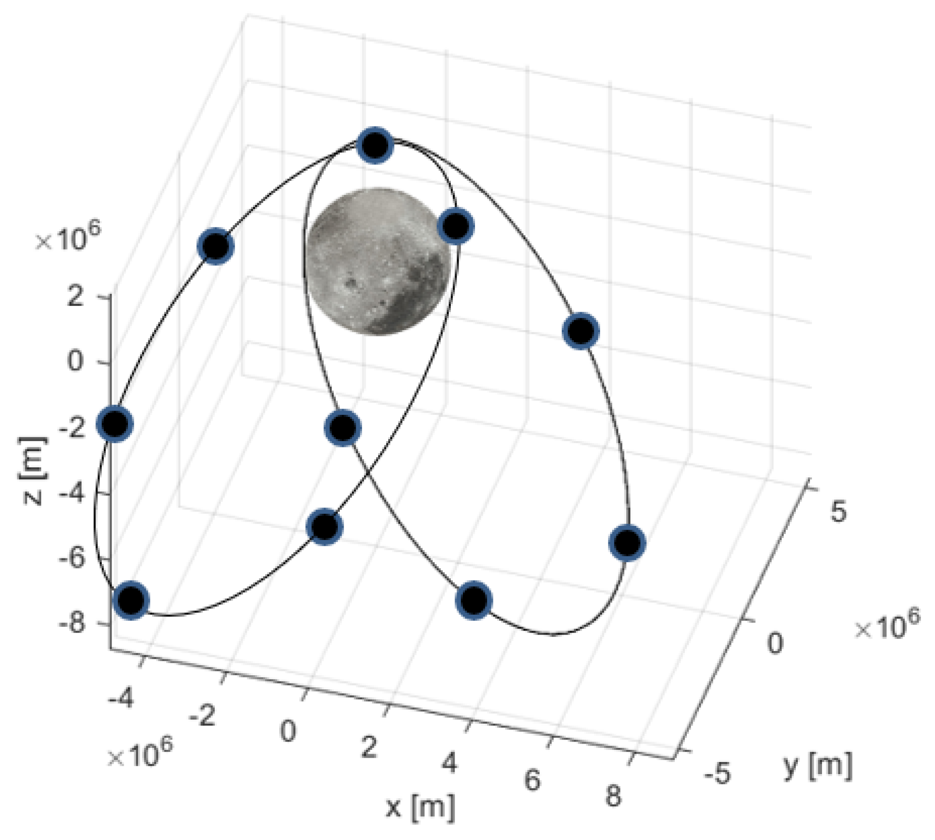
The orbits of an ELFO are illustrated in Figure 1 and the parameters are contained in Table 1. The orbital period is approximately 19 h and provides strong coverage of the Lunar poles during the apogee, where the South Pole is chosen. An ELFO can also vary in the right ascension of the ascending node, so satellites can be placed across different planes. For a navigation service in particular, this is highly beneficial to improving visible satellite geometry.
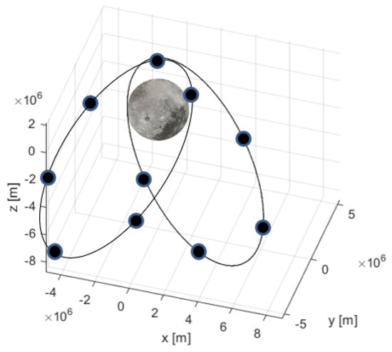
Figure 1.
Trajectory of the evaluated lunar navigation constellation in ELFO.

Table 1.
ELFO orbital parameters.
The number of satellites and plane separation in Figure 1 are just for illustration purposes. Work by [7] has optimised for either nine satellites distributed across three ELFO orbital planes or ten satellites across two planes. In this work, the 10-satellite distribution is used.
It is important to note that these parameters are established in the Moon’s Mean Earth (ME) frame [26,27], and not in an inertial frame as for Earth-originated Kepler parameters. The position and velocity are solved by the general conversion equations from Kepler to Cartesian [28], and then transformed from the ME to the J2000 frames.
2.2. Satellite Design
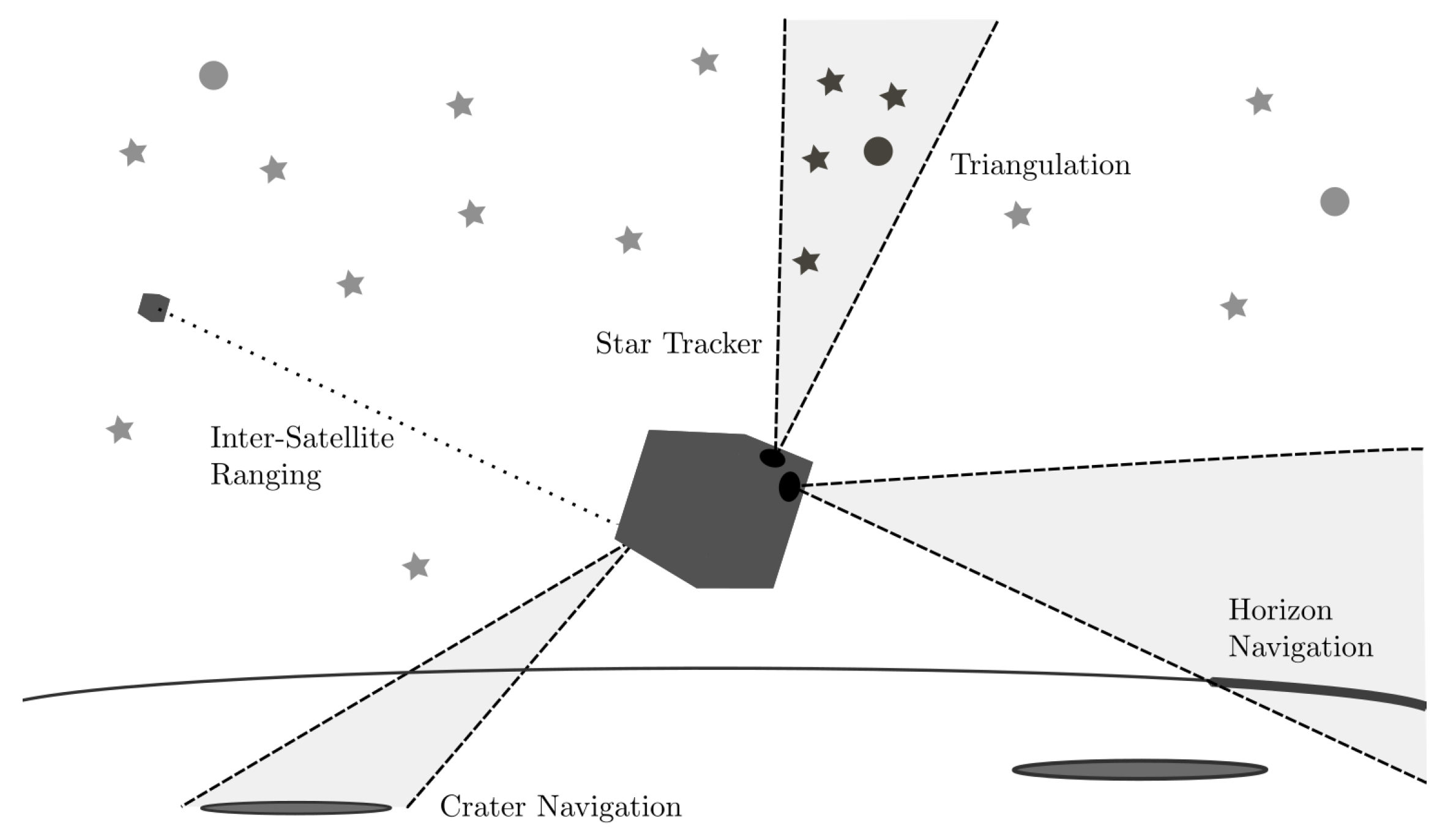
As introduced, five different types of guidance and navigation sensors are evaluated in this work: star tracker, horizon navigation, triangulation, crater navigation, and inter-satellite ranging. Each of the techniques are illustrated in Figure 2.
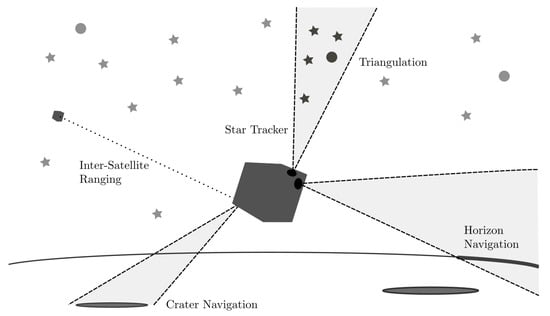
Figure 2.
Concept of potential navigation sensors for an autonomous lunar navigating spacecraft, including star, horizon, triangulation, crater, and inter-satellite ranging techniques.
For each optical-based sensor, which encapsulates all except ISLs, parameters of a standard space-rated, commercial off-the-shelf camera are treated. Cameras are very common to most lunar missions, and so impose no cost to the satellite architecture. However, they may constrain the satellite design. Each sensor is assumed to be positioned on the spacecraft at an attitude that is in constant view of the target. Reorientation of the satellite during flight is ignored.
Potential design limitations of each proposed sensor are introduced in Table 2. It is immediately obvious that not all sensors could be used simultaneously, due to pointing requirements, as well as general size, weight, and power constraints for a small spacecraft. However, a carefully managed integrated approach might be possible, overcoming the specific challenges of each.
Table 2.
Spacecraft sensor choice design implications and challenges to performance.
3. Proposed Sensors
In this work, various celestial-based sensor systems, as well as inter-satellite links, are proposed and models presented. Derivations are not incorporated in this work, as the paper focuses more on implementation and performance. Celestial sensors include star trackers, horizon, point source triangulation, and lunar craters.
3.1. Star Tracker
The star tracker is a highly accurate and technologically mature attitude determination sensor common to most spacecraft architectures. The star tracker is critical to any autonomous orbit determination architecture, and so will be briefly discussed. Given the high number of books and articles in the literature discussing star trackers [29,30,31], the reader is referred to them for further learning.
In short, the star tracker captures images of the night sky, and by identifying star patterns using astrometric databases, typically by comparing angles between neighbouring stars, an attitude can be calculated between the sensor’s body and the inertial, celestial frame. The process of star identification is complex, with sophisticated algorithms adopted to compare many star patterns, so false identification is avoided. Any small risk of a star being misidentified leads to it being rejected (usually below 0.01%). Popular algorithms include Pyramid [32], which compares star patterns by constructing and measuring a pyramid-like geometry, and Tetra [33], which identifies stars to a catalogue by using a hash code.
In this investigation, the star tracker is treated as an accurate attitude determination source with a precision of approximately 10 arc-sec [15]. This will be delivered by an instrument with a 20° field of view with a pixel resolution of 1024 × 1024 px. This is typical of most common star trackers [34].
The attitude of the sensor represents the orientation of the sensor body frame B with respect to the inertial celestial frame I, expressed in the form of an attitude transformation matrix . This is important in transforming Moon features, such as the horizon or craters, to a local planetary frame of the body, P. Any attitude error will directly impair the navigation performance, as is highlighted in later sections of this work. The transform between the inertial and planetary frame is known by international scientific working groups and organisations, such as International Earth Rotation and Reference Systems Service (IERS), and so the body to planetary frame transform is calculated by .
The transformation matrix between the celestial and planetary frame has been accurately modelled for the Moon, using measurements from recent missions such as the reconnaissance orbiter [27]. In this paper, it is assumed that any error in the model is negligible, as typical inaccuracies are far below the star tracker performance of 10 arc-sec.
The calculated attitude will also include a slight angular bias, caused by mechanical misalignment and thermal fluctuations of the satellite platform. This bias will slightly rotate the attitude transformation matrix by an angle , generating an offset between different sensors. The misalignment can be described by multiplying a Direction-Cosine Matrix (DCM) of to , i.e. .
This bias is addressed by employing multiple optical sensors that may usually measure the horizon, distant object triangulation, or craters as a star tracker, where the hardware remains the same but the software loop is changed. In this case, the misalignment factor between the two sensors can be estimated up to the performance of each sensor acting as a star tracker. The performance of this correction is estimated to be 0.01° [35,36], and so this will be used as the angle in this work. It is important to note that this estimate would require both sensors to have a star field in view, and so spacecraft pointing would be required.
An alternative methodology to reduce the misalignment error is proposed by Mortari in the StarNav III solution [37], where three separate star tracker lenses share the same sensor. This is delivered by a complex series of lenses and mirrors to transfer the observed star field photons to a single camera sensor. A similar approach may be used where celestial observation may also be transferred to a single sensor. Even if the error reduction is not negligible, given the complexity of the proposed system, it is not treated in this work.
3.2. Horizon Navigation
The sextant is an ancient tool for navigation, and in the early days of the space race, it was considered to be one of the primary sources of positioning by astronauts [38]. Modern techniques have vastly improved its performance and applicability [11,39], being treated in both cislunar and Earth orbits. The application of the techniques developed are treated for the lunar context.
Both the Moon and Earth can be modelled as an ellipsoid. This treatment is suitable for distances of more than 100 km above the surface [15,40], where rugged terrain does not exceed 10 km, with a standard deviation of below 3 km. It is thus not visible on the horizon projection in most wide-field-of-view lens assemblies for systems in orbit.
A point on the surface of the planetary frame can be expressed by
with radial dimensions a, b, and c. Alternatively, it can be expressed in matrix form:
where is the ellipsoid body matrix. The Moon can be approximated as a sphere, where , and the Earth as an oblate spheroid, .
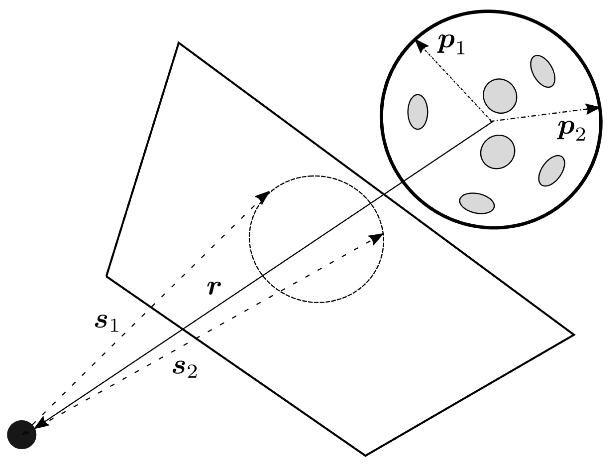
An illustration of the ellipsoid and the projected shape on a camera sensor is reported in Figure 3. The projected shape may either be a circle, ellipse, parabola, or hyperbola, depending on the conic section created by the ellipsoid. The general quadratic equation describes a conic section in the body frame with measured image coordinates ,
where are coefficients. A similar matrix form could be written for this projection, writing a vector that would intersect at a tangent with the ellipsoid surface, as
The vector can be transformed to the planetary frame using the estimated attitude transformation matrix in Section 3.1.
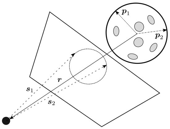
Figure 3.
Ellipsoid as seen by the spacecraft in the camera sensor body frame.
Errors in the estimated horizon point, such as stray light, optical noise, or large rugged terrain, are introduced in the estimated limb pixel . The estimated performance of a measured horizon coordinate can be assumed to be 0.1 px [11,36,40]. It is suggested that upon implementation the optical system hardware developed reflects this estimation resolution.
These two expressions can be related to the sensor position , measured from the ellipsoid origin, by where d is some scalar multiplier. These two functions can be then simplified by an approach given in [39] to
where
Matrix M describes the shape of the projected ellipsoid on the image sensor, as a function of the ellipsoid matrix A and the observer position . This term is equivalent to the ellipse matrix, as represented in Equation (4), which can be denoted by C, by the following generalised eigen-problem expression,
where is an eigenvector and is an eigenvalue.
It should be noted that the frame subscript has been dropped in Equation (6). It is important that all matrices and vectors are in the same frame, i.e., body, inertial, or planetary. This expression can be used for estimation of the position in an implicit least square-based model.
Work by [17] treats the celestial horizon in Cholesky space, which reduces the problem from a non-linear to a linear case. However, the handling of errors in a fused Extended Kalman Filter (EKF) is problematic, as it is challenging to map the measurement noise to the Cholesky space geometry. The non-linear case is used in this work.
The performance of the horizon estimation algorithm is illustrated in Figure 4 for a changing altitude above the lunar surface. For this evaluation, a star tracker with a precision of 10 arc-sec is treated, as was described and proposed in Section 3.1. The horizon sensor will have the same resolution and sensor shape, with 1024 px in both horizontal and vertical directions. The field-of-view size is, however, 40° to encapsulate more of the lunar arc.
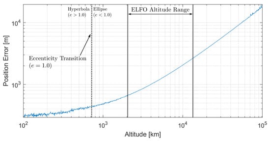
Figure 4.
Horizon estimation performance at varying orbital altitudes, with the eccentricity transition and ELFO altitude range highlighted.
In Figure 4, the ELFO orbital altitude range is indicated from 3026 km to 10,210 km. The transition between a hyperbolic and elliptical projection is also highlighted, and it does not fall within the orbital altitude range of the ELFO, occurring at 707 km.
From Figure 4, altitudes beyond the ELFO operating range appear unsuitable for this application using horizon-based navigation, moving towards accuracies of more than 3 km. Within the operating range, performance varies between approximately 650 m and 3 km. It is suspected that this is caused by changes to the visible length of the lunar limb, with a constant camera resolution, at various distances from the surface. At altitudes below 300 km, the horizon approach plateaus as meaningful curvature information is no longer measurable. Results below 100 km have been omitted for this reason.
Visibility of the Moon as it changes from day to night will affect the performance of optical navigation. The visible lunar limb arc will predominantly stay the same; however, the length visible to the spacecraft will depend on the camera’s attitude. For the purposes of this study, the lit limb arc will be assumed to always be half the lunar disc’s circumference. Except at full and new Moon, this will always be the case. However, this makes an assumption that the camera’s attitude will be placed to ensure that the maximum arc is visible.
3.3. Triangulation
Triangulation modelling has been the subject of study for millennia, with cases from the Egyptians and Greeks of using the concept of a triangle to measure distance and size. A historical review is provided in [41], treating records of the Greek mathematician Thales estimating pyramid heights and ship distances at sea, and of Hipparchus estimating the distance between the Sun and Moon. Modern understanding is first accounted for in the 1600s.
Techniques of triangulation are mutually inclusive to well-known direction or Angle of Arrival (AOA) position estimation, as is common and highly mature in maritime [42] and aviation [43] fields using radio-based measurements. This topic has been considered more recently in the context of indoor and wireless navigation [44]. The measurements are typically confined to a two-dimensional plane.
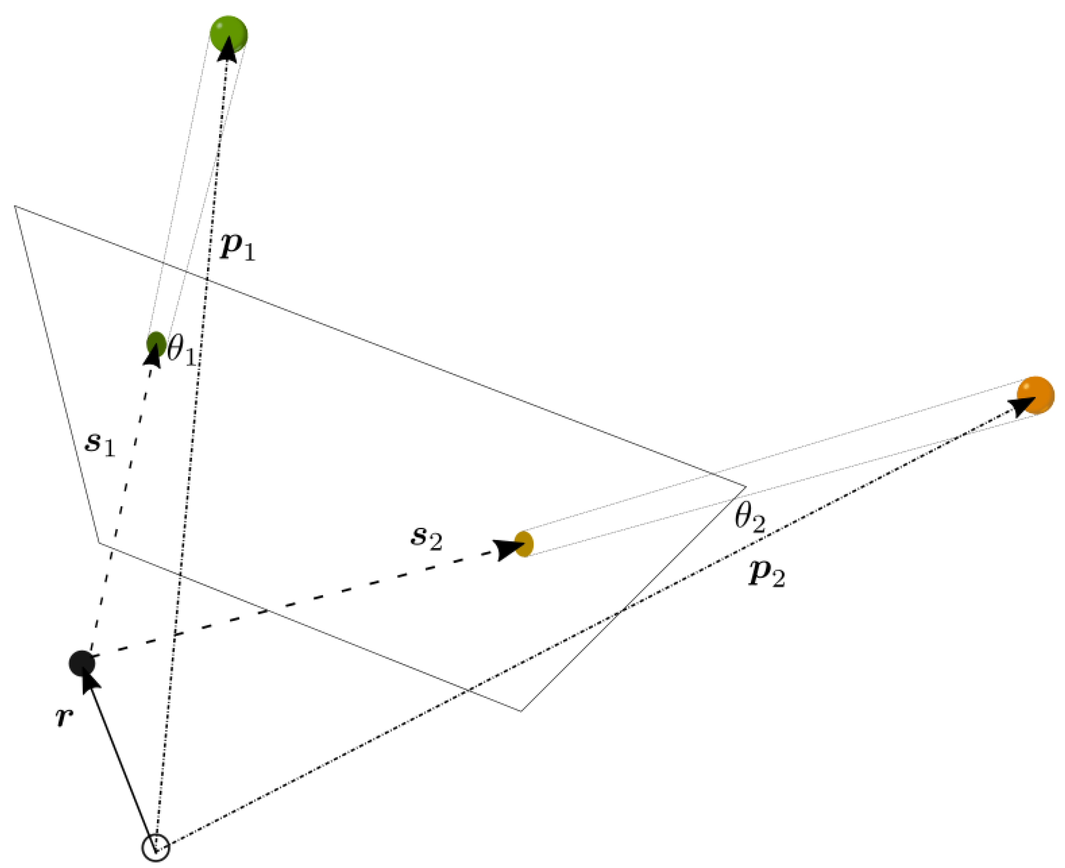
A representation of the celestial sphere through an AOA approach is illustrated in Figure 5. The celestial body position is located at and the observing vector at . A familiar relation can then be established, , as in the case of the horizon. The angle of arrival can be calculated from the dot product relation, . This relation is used by [41].
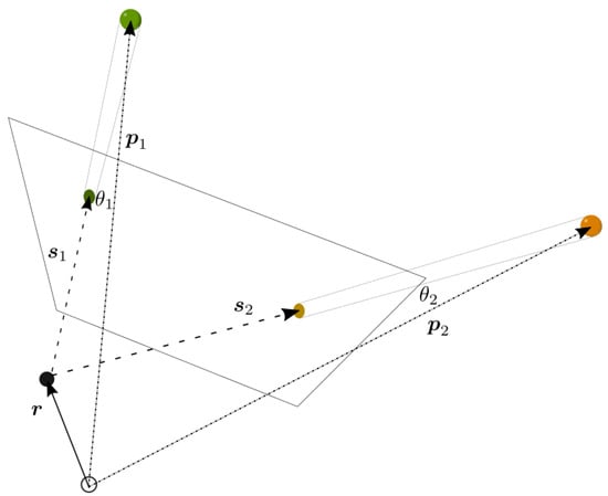
Figure 5.
Distribution of planetary point sources at positions with trigonometric relationships to a spacecraft at , measured by .
To explore the potential performance of triangulation techniques in space, this relationship can be reduced to the two-dimensional plane, like for wireless or indoor positioning. Using a measured angle from the ith source at , the relationship between position and the celestial source is a simple tangent trigonometric function [44],
For a multiple number of sources, this model may then be solved for and as a determinable system.
In AOA radio-based techniques, the geometry of the observation sources is typically treated as an indicator of performance. Known as the Dilution of Precision (DOP), it is calculated from the measurement matrix, providing a relationship between the measurement noise and the position error . For the purposes of this work, the DOP should be expressed in the form of
The DOP may be derived in terms of an angular measurement by first taking the derivatives of Equation (8) in terms of and ,
where . This may be written in matrix form as
for m observed sources. The DOP is then calculated as .
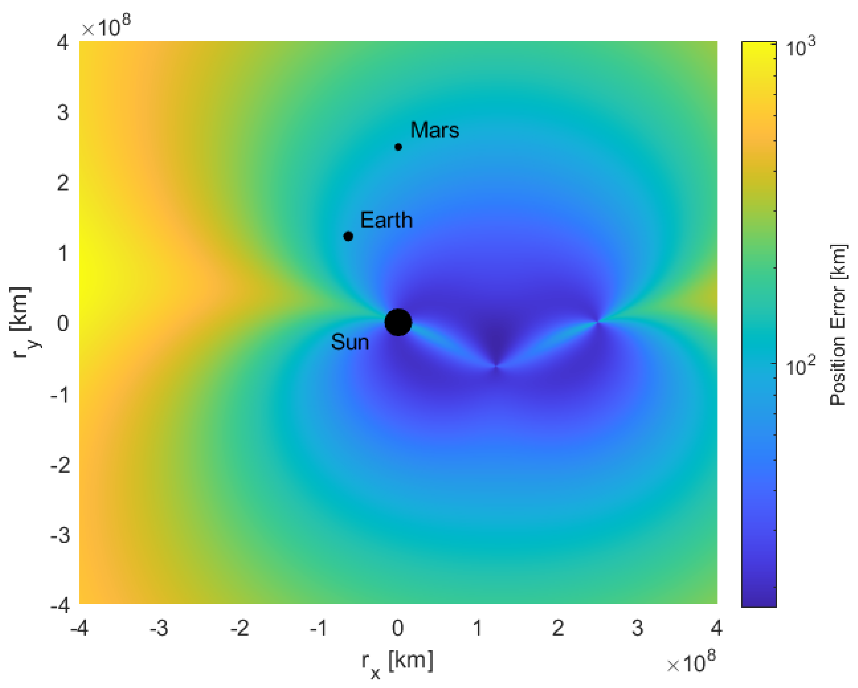
The DOP, and thus calculated position error, can be considered in the solar system plane. In Figure 6, the Sun, Earth, and Mars are treated as an observed distant celestial source at a position . In this example, the sources are placed in one quadrant of the solar system plane, with the Sun at the centre. For a spacecraft at some position in the plane, the expected position error may be estimated by first calculating the DOP from Equation (11), and then the position error by Equation (9).
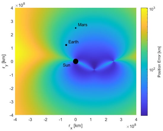
Figure 6.
Position error of a spacecraft at a position in the solar system plane with origin at the Sun, using triangulation from the Sun, Earth, and Mars with an object localisation accuracy of 0.01°.
The error in Figure 6 is illustrated up to a distance of 4 × 10⁸ km from the Sun, where each celestial source is measured by the sensor up to an accuracy of 0.01°. This is similar to the performances delivered by the star tracker described in Section 3.1, where the technique of measuring each celestial body source is very similar.
These results make an assumption that the planets are constrained to the solar system horizontal plane. The DOP of the plane varies from 108 to 1010, and thus the illustrated best case position error would be 10 km in certain regions, moving towards 1000 km in others. This performance would be unsuitable for localised orbit determination, but perhaps is applicable for navigation in interplanetary travel.
3.4. Crater Navigation
Using craters for navigation around the Moon, alongside other planetary bodies, was initially considered in the context of asteroid rendezvous [45,46]. Likening them to ellipses, similar approaches to horizon ellipse fitting have been developed for location pinpointing and crater identification.
Crater estimation techniques have received significant renewed interest in the context of lunar exploration [47,48]. This technique has been especially considered for the case of lunar descent, where decimetre performances are usually targeted [16,49].
The work of Christian provides a linear least-square estimate for the general crater positioning estimation problem and will be used here [47]. Traditional crater identification algorithms have been studied [50], but machine learning and Artificial Intelligence (AI) present higher performances, popularly adopted by [16,47,51].
Many databases have been generated by various recent lunar missions, including the NASA Lunar Reconnaissance Orbiter and Chinese Chang’e Lunar surveyor, as well as by ground-based astronomy. The simple database created by the Lunar and Planetary Institute is used in this analysis. Even though craters are described as circular, the projections on the camera frame provide appropriate ellipse shapes for fitting to be evaluated, and position error estimated [52].
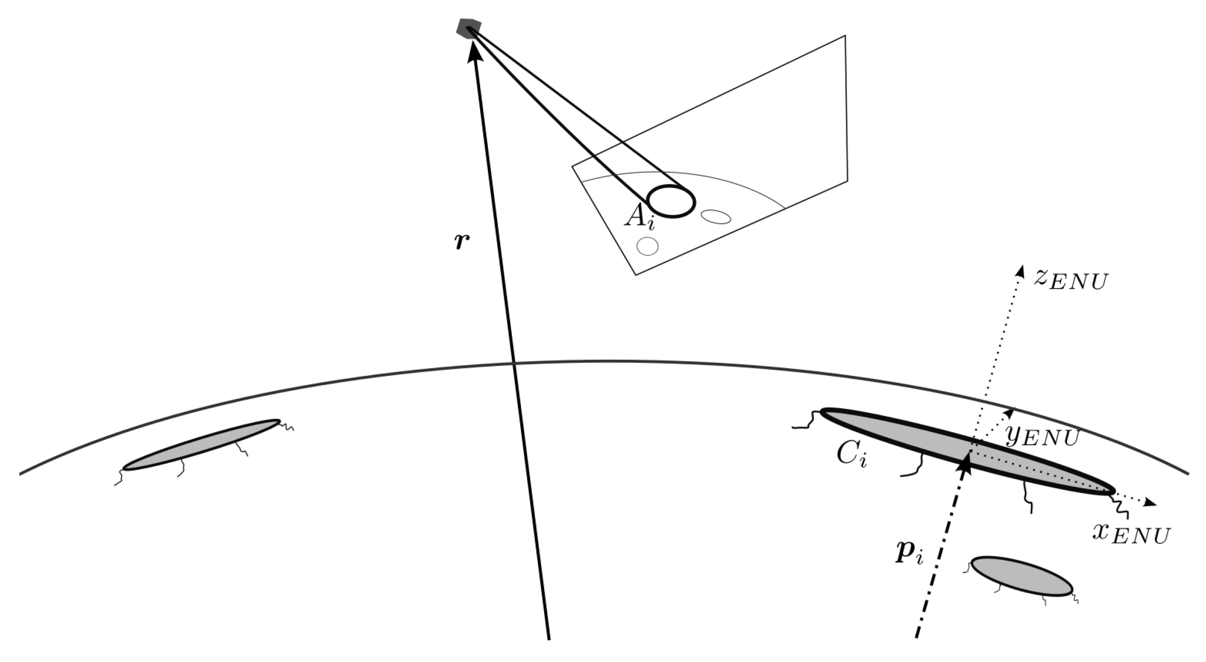
In crater-based navigation, three different references are treated, the optical sensor body frame B, the lunar planetary frame P, and the local East-North-Up (ENU) frame of the crater E. The transformation between the body and planetary frame is known by the star tracker, as introduced in Section 3.1.
The crater ellipse projection is developed in a similar fashion to the horizon, and is illustrated in Figure 7. The profile can be expressed by Equation (3), where the crater i measured across the image plane can be denoted by a matrix . This is after a set of image points is fit to an equivalent ellipse by a routine first proposed by Fitzgibbon [53], providing a set of conic coefficients, . The approach also provides a covariance with the associated non-linear least-square estimate, which is expressed as a matrix .
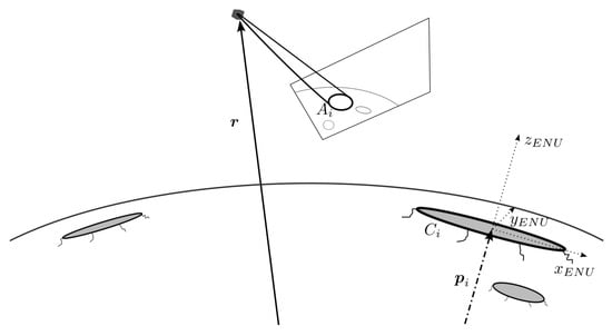
Figure 7.
Lunar craters projected on a spacecraft’s camera lens.
Similarly, the shape of the crater is known within the crater database by the shape matrix , defined as in Equation (4). The ellipse is defined in the crater’s local ENU frame , centred at the ellipse origin in the Moon’s planetary frame. The ENU frame is highlighted on the projected equator in Figure 7. The ellipse relation between and , after appropriate identification by a machine learning algorithm [16,51], can be related through a series of projection transformations for the spacecraft located at a position [47].
Defining first the homography for the ith crater,
where is the transformation matrix between the fixed lunar planetary and crater’s local ENU frame, and S is a matrix,
The transformed measured crater in the lunar planetary frame is calculated by
where any focal length-related parameters can be related by some scalar . The relation between and is then given by
where .
This expression might be rearranged to matrix form for the left-hand side as
The independence of the matrix upper-left hand corner to the spacecraft position vector can be used to find the scalar as the least squares-like solution,
where the operator converts a matrix into a vector, with each column of the matrix ‘stacked’ on top of the other. The upper-right-hand corner of the matrix in Equation (16) can then be used to create a linear system in terms of the spacecraft position vector for m craters,
The visible craters on a standard lunar projection are highlighted in Figure 7, where each corresponding projected ellipse matrix to a corresponding crater ellipse is plotted.
The associated covariance of each measurement may be calculated by the ellipse coefficient covariance . The associated covariance measurement model covariance matrix is calculated by
The position covariance estimated is then
These derivatives can be simply solved by performing a vector derivative on Equation (18).
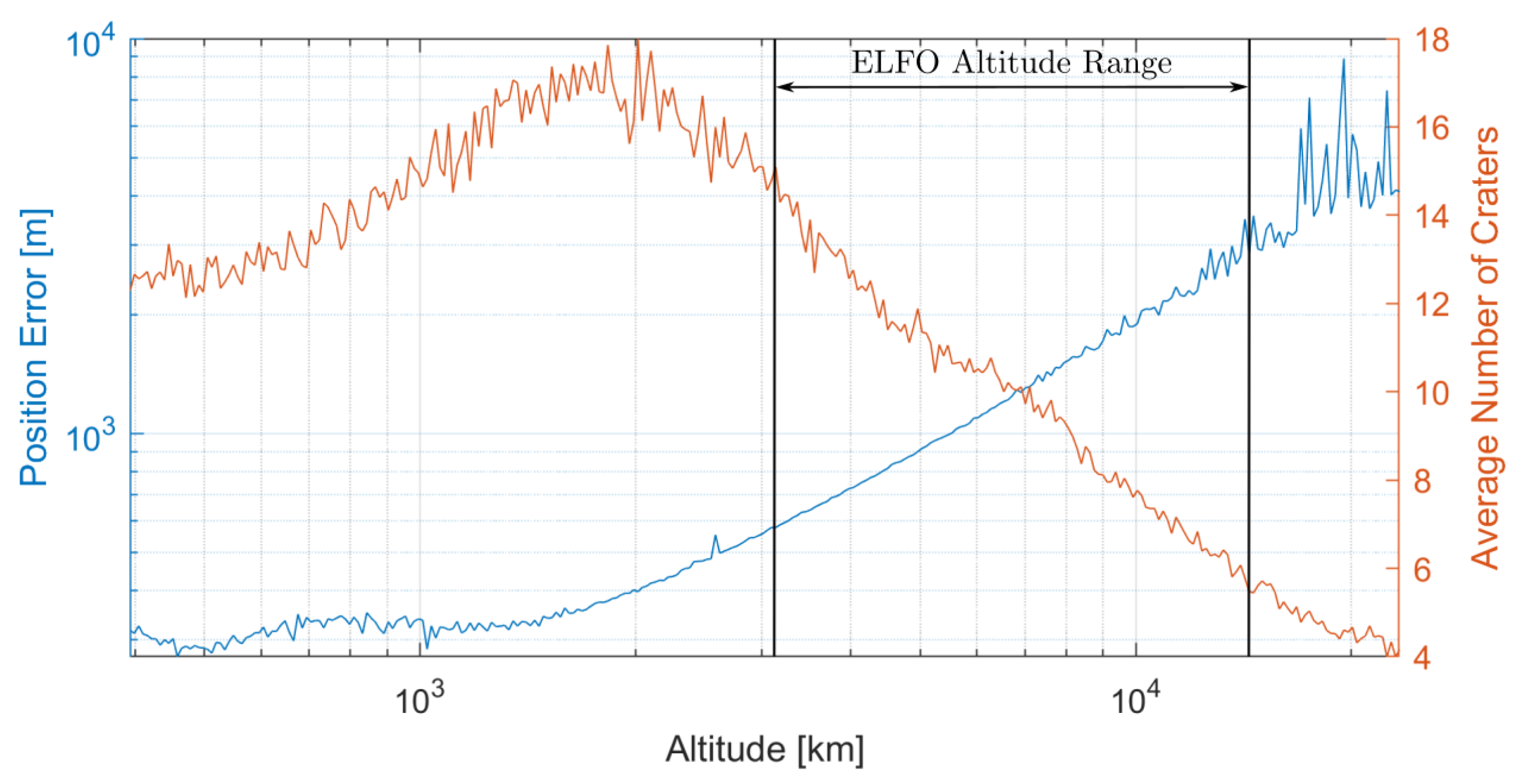
The position estimation performances of crater navigation at varying altitudes are illustrated in Figure 8. A sensor similar to the horizon sensor is treated, with a 40° field of view and a resolution of 1024 px. Each performance in Figure 8 takes an average of 100 position estimates at randomised lunar rotations. These results are juxtaposed by the average number of craters identified, which can vary by not only altitude but also the side of the lunar surface visible. The lunar far or dark side, being the side opposite to the tidally locked face, has a higher number of impact craters given that it is less protected by the Earth.
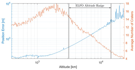
Figure 8.
Crater estimation performance alongside average number of visible craters, at varying orbital altitudes, with the ELFO altitude range highlighted.
Performance of the proposed crater technique increases as the spacecraft nears the lunar surface, as more craters become identifiable. It then plateaus at 1000 km above the surface, at a performance of approximately 200 m. This however might be caused by the elliptical fit approach of this work. AI techniques, which can provide more accurate identification fitting, might significantly improve the result. The camera optics are also constrained.
Within the ELFO operating range, performances of approximately 1 km to 12 km are witnessed in Figure 8. This variation is not appropriate for autonomous positioning, and may also present challenges to the EKF since the estimated covariance will change significantly.
Craters are only visible when the sun is overhead, down to an angle of elevation of approximately 20°. This constraint may be maintained by taking the dot product of the sun and crater unit position vector in the lunar fixed frame, , where the hat indicates it is a unit vector.
In this study, 70° is taken as the angular limit between the sun direction and the crater normal; otherwise, it is treated as too dark to be detectable. This may further reduce performance, and is accounted for in the studied orbital propagation and filter scenarios of Section 4.
3.5. Inter-Satellite Ranging
Utilizing inter-satellite communication links for ranging has grown increasingly popular in recent years given the rise of mega-constellations, a climbing demand for ground stations, and a growing desire for autonomous satellite operations in the face of threats. ISL ranging was treated early for improving performances to the GPS [54], and could similarly be considered for an LCNS. The ISL range limit is 4500 to 45,000 km [55], and the link separation will not exceed this range in the analysis of Section 4.
Managing ISLs with multiple satellites has been proposed by numerous authors for an LCNS [18,19,56,57]. Each follows the same ranging signal model structure, typically measuring a distance between neighbouring satellites ,
where and is the position vector of some satellite indexed by i or j. The management of the ranging set by multiple neighbouring satellites is described in Section 4.2.
Similarly, the Doppler signal may be measured to deliver a satellite velocity estimate. This would require the relative velocity v of the satellite j, leading to the following model,
Given that the velocity information is unknown from any other sensor treated in this work, the solution would be highly valuable.
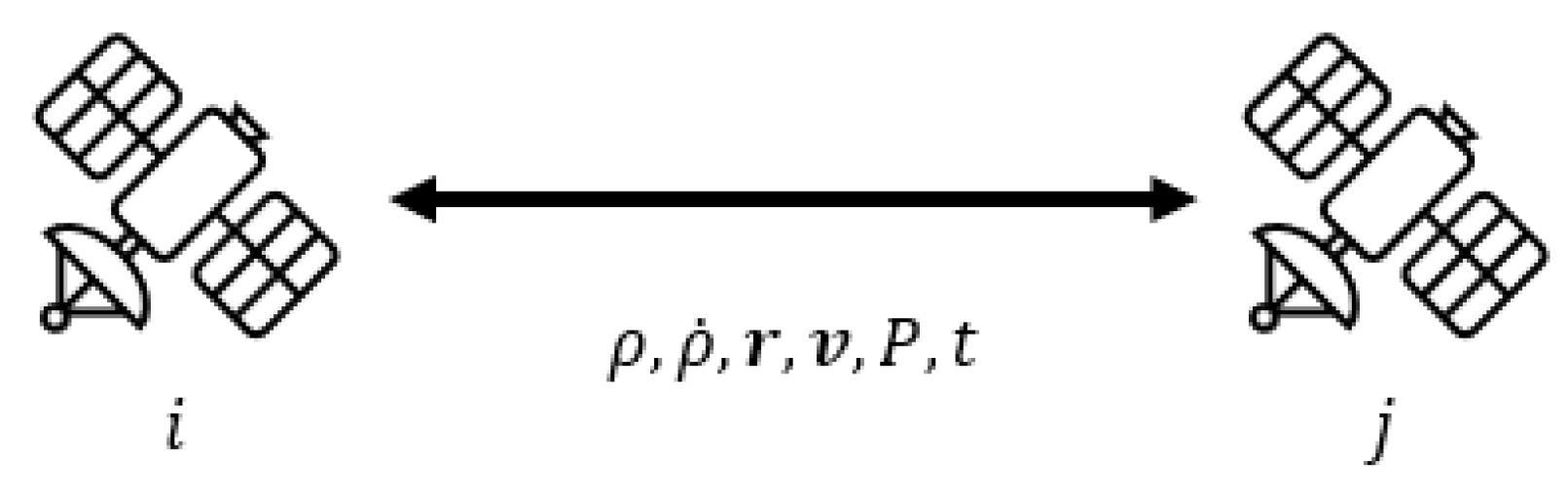
The range and appropriate position covariance should be transferred between satellites. This transfer is illustrated in Figure 9 and should be communicated through the link. P denotes the covariance of the position and velocity estimates, and t is the time information of the transmitted position and range.

Figure 9.
Inter-satellite link information transfer between satellites i and j. The t indicates the transfer of time information.
The ranging performance of the inter-satellite links is conservatively set to 6 m and 1 mm/s. This is close to the higher bound of those parameters used in the literature [56,57]. It should be noted that this technique only provides a relative position and velocity between spacecraft, and is dependent on other techniques to provide a sufficient absolute accuracy. It cannot be used independently but can enhance performance. Performance analysis of this technique is deferred to Section 4.
4. Lunar Orbital Filter
This section describes the implementation of lunar orbit propagation filter sensor fusion techniques. Performances are then presented, alongside trade-offs for their implementation. The desire is to deliver a precision of 30 m, as has been previously discussed.
4.1. Orbital Propagation
Orbital dynamics with third-body perturbations have been studied since the Apollo program [58], but considerations of a permanent orbiting service infrastructure are more recent. The frozen orbit, a mathematical outcome of three-body dynamics where gravity perturbations are minimized in certain orbital configurations, was proposed and explored more recently in the 2000s for the Moon by [26]. The ELFO is one such configuration, where LunaNet [4], Moonlight [5], and the Japanese LCNS [6] have all utilised this orbital ‘anomaly’ within their system architecture.
The three-body problem is notorious for not being solvable algebraically. However, techniques have been developed to provide a numerical estimate. The Runge–Kutta four-step method is applied in this instance for calculating the propagation from time step k, , to time step , [59], which is reasonable for accuracies targeted in this work. However, a linear approximation is required for most filter-based solutions,
where is a vector-valued function to calculate the propagation, and is the linearised matrix form of , the propagation matrix. In this work, the state vector is composed of .
The acceleration of the spacecraft is caused mostly by gravitation forces from the Earth, Sun, and Moon, as well as solar-derived forces, such as radiation pressure and wind. Typically, for a small spacecraft orbiting the Moon, the resulting acceleration by the solar radiation pressure is in the order of 1 × 10⁻⁸ m/s2 [60]. Solar wind is even less, causing accelerations at 0.5 AU from the Sun to 1 × 10⁻¹¹ m/s2 [61]. At this stage, solar-derived forces are not treated, as this work focuses on a covariance analysis to predict expected levels of accuracy with a proposed set of measurements, and not on dynamic model performance.
Both the gravitational field of the Earth and Moon cannot be treated as point masses. Spherical harmonic models have been developed to a high level of fidelity, where the Earth Gravitational Model (EGM) provides a 2160-degree harmonic for the Earth [62] and the GRGM900C provides a 900-degree harmonic for the Moon [63]. To reduce processing time, with an assumed negligible loss in performance (on the order of 1 m per day [28]), the EGM and LP160C [64] models have been reduced to two-degree and four-degree harmonics for the Earth and Moon, respectively.
These models are taken from Montenbruck for Earth-based orbital GNSS [65] and applied to the lunar domain. A point mass assumption is established for the Sun, using the Newtonian gravitational acceleration equation,
where G is the gravitational constant, is the mass of the Sun, and is the vector pointing from the spacecraft to the Sun. The relation between and is .
The gravitational accelerations of the Earth, Moon, and Sun, , and , respectively, can then be added together to calculate the acceleration. The time derivatives for the state vector are written as
Each is calculated as a function of the state , .
As mentioned, for filtering techniques, a linear solution to the non-linear propagation function must be first derived. This may be calculated through a linearised form of the dynamic model , where the linearised form is the dynamic matrix F. A solution to the propagation matrix is , where is the time between step k and [28].
To calculate the dynamic matrix F, the derivative for the gravitational acceleration for the Sun in terms of , should be calculated
The chain rule may then be applied to find the derivative in terms of the state vector term ,
which uses the relation . Similar forms may be computed for the Moon and Earth gravitational equations. For spherical harmonics, the solution is more complex. The reader is directed to [66] for the non-spherical gravitational Jacobian. The remaining terms forming the dynamic matrix are
4.2. Kalman Filter Application
The Kalman Filter has been well-developed in the literature [39,67,68,69], starting in the 1960s and extensively used across many positioning and navigation scenarios. The basic equations are provided for the sake of completeness. The measurement vector is dependent on the sensor used, as described by the architectures proposed in Section 3.
The propagation update of the EKF for the state vector and the estimated state covariance P is described by
where the propagated linear approximation matrix was first defined in Equation (23). The propagation update error covariance is described by the matrix Q.
The measurement update of the EKF is given in an implicit form to accommodate for the measurement model of the horizon, as in Equation (5). This means the measurement model is of the form , where is the measurement vector. This is then applied to the basic measurement update equations of EKF as
where the superscript + highlights the state and covariance estimate post-measurement update, I is the identity matrix, R is the measurement noise matrix, and H is the linearised form of the measurement model . The measurement noise matrix is calculated by taking the partial derivative of the measurement model in terms of the measurement vector and performing a matrix multiplication by the predicted sensor noise ,
Similarly, the measurement matrix H is calculated by the partial derivative of the measurement model by ,
Two options exist to manage the combination of multiple sensors. The first is to combine the measurements to a single measurement vector . This approach is classified as simultaneous data fusion. For example, the combination of horizon points and lunar crater ellipse estimates, captured by the same camera, would take the form
The measurement model vector , measurement matrix H, and the measurement noise matrix R would be then expanded to include both models as separate blocks.
The alternative model is to consider various points of sensor information separately, independently propagating and estimating with measurement steps as each signal is received. This is known as sequential data fusion and is more practical if different sensors return measurements at different time steps. For each measurement, Equations (31)–(33) are followed. Kalman Filter data fusion research does not follow conventions, so this difference is highlighted.
A challenge to sequential data fusion arises if there is a significant difference in sensor noise, especially at varying time steps. This may take place, for example, if the observed lunar crater or horizon geometry changes between apoapsis and periapsis. This would lead to a radical change in the performance, and either sensor information should be ideally scheduled when performance is sufficient, or weights must be applied to reduce the impact poor-quality data may cause in the estimated position.
One approach is the federated filter, which is described in detail in [68] and is usually applied to automotive sensor fusion. The combination of the separate filter terms to the master filter m is given by
where state and covariance information is given for a set of sensors. The importance of one sensor over another is given by a weight , where the covariance matrix is multiplied by this weight term on each time step k, i.e., . The covariance propagation update Equation (30) is also modified as
The weights should reflect the mean inverse average , so,
and should be within .
When handling inter-satellite links, the noise of the measured range must be transferred between satellites. The approach, known as a Decentralised Schmidt EKF [18,57], combines the covariance from the current and neighbouring satellite within the measurement update. Equations (31)–(33) are rewritten as
where is the derivative of satellite i’s measurement model in terms of its own state, is the derivative of satellite i’s measurement model in terms of satellite j’s state, i.e., , and is a new covariance matrix of the two satellite combined states, with .
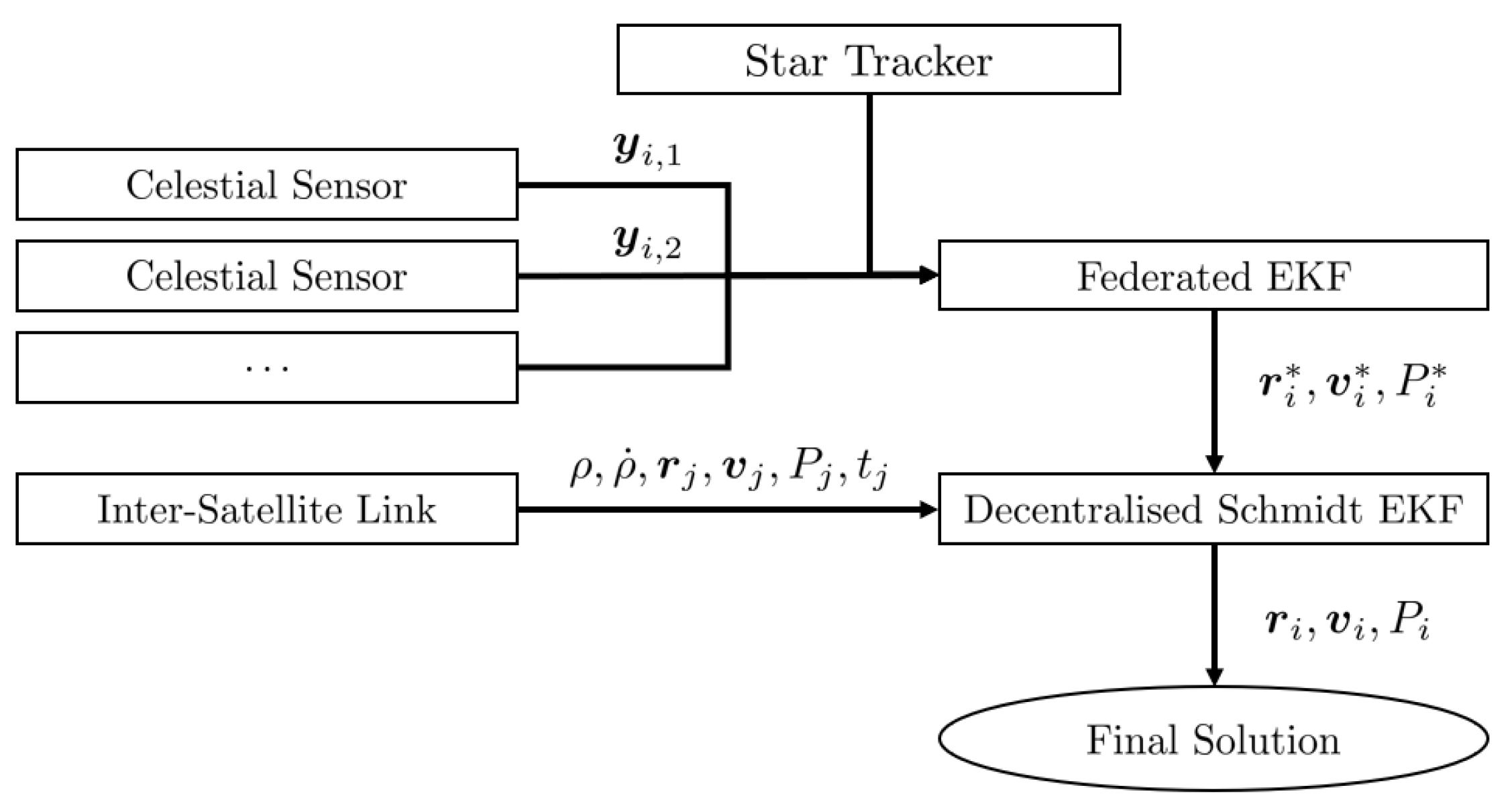
The combination of sensor models and the two proposed Kalman Filters are illustrated in Figure 10. The orbit propagation element is included within each EKF box and follows the procedure described in this subsection. Celestial sensors are fused by the Federated EKF for some satellite i, followed by any ISL measurements from a satellite j integrated using the Decentralised Schmidt EKF.
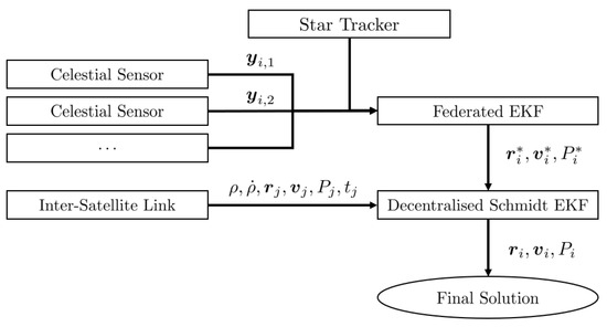
Figure 10.
Sensor and Kalman Filter model illustration.
4.3. Kalman Filter Performances
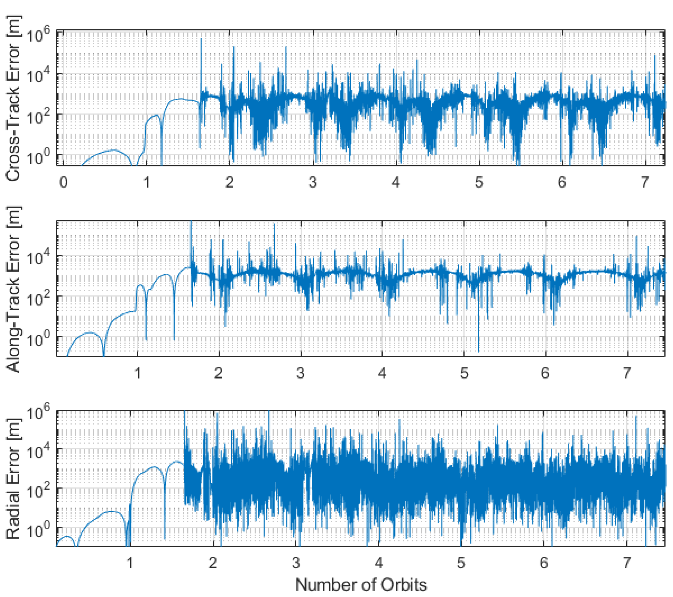
The proposed filter methodology is evaluated, considering various sensor combinations. The performances are presented in Table 3. Sample EKF results for a horizon-based and crater-based-only navigation filter are illustrated in Figure 11 and Figure 12, respectively. Weights are used of 1.01 and 101 for the lunar horizon and craters respectively. An increase in noise is associated with distance to the lunar surface.
Table 3.
EKF for position sensor combinations at 1.
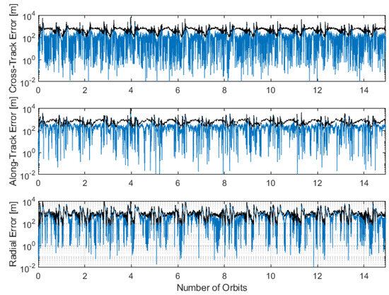
Figure 11.
Lunar- horizon-only EKF position error for a spacecraft in ELFO. The error is in blue and the black illustrates the solution boundary at .
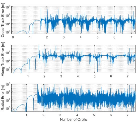
Figure 12.
Lunar-crater-only EKF position error for a spacecraft in ELFO. The error is in blue.
Each performance is insufficient to satisfy the positioning objectives of an LCNS, with errors in the range of 100s of metres. Of note is the low accuracy of the lunar crater model, with a performance from 1 km to more than 20 km. This is due to the high variability of performance based on lunar surface proximity, as was illustrated in Section 3.4. This presents a challenge to the covariance model within the filter. The variability of the lunar horizon accuracy with altitude is much less, and so the EKF precision stabilises.
Performances with a fused horizon and crater-based filter are also highlighted in Table 3. The performance overall is worse than the horizon-only model, which is most likely caused by the high variability in crater performance to altitude. The crater technique is worse in the radial direction than on the cross- and along-track, which also affects the combined solution. Interestingly, the precision is much stronger using the combined measurements, indicating that any solution bias is reduced. This makes sense as the crater technique uses points over a wider geometrical spread than the horizon, which is restricted to the Moon’s corners.
Such a fusing may help in lunar ellipse or other poor limb-lighting conditions. In addition, if satellite pointing does not capture the limb perfectly but only the surface, the crater form could also be used to assist in stabilising the filter. Challenges to each sensor’s performance are highlighted in Table 2.
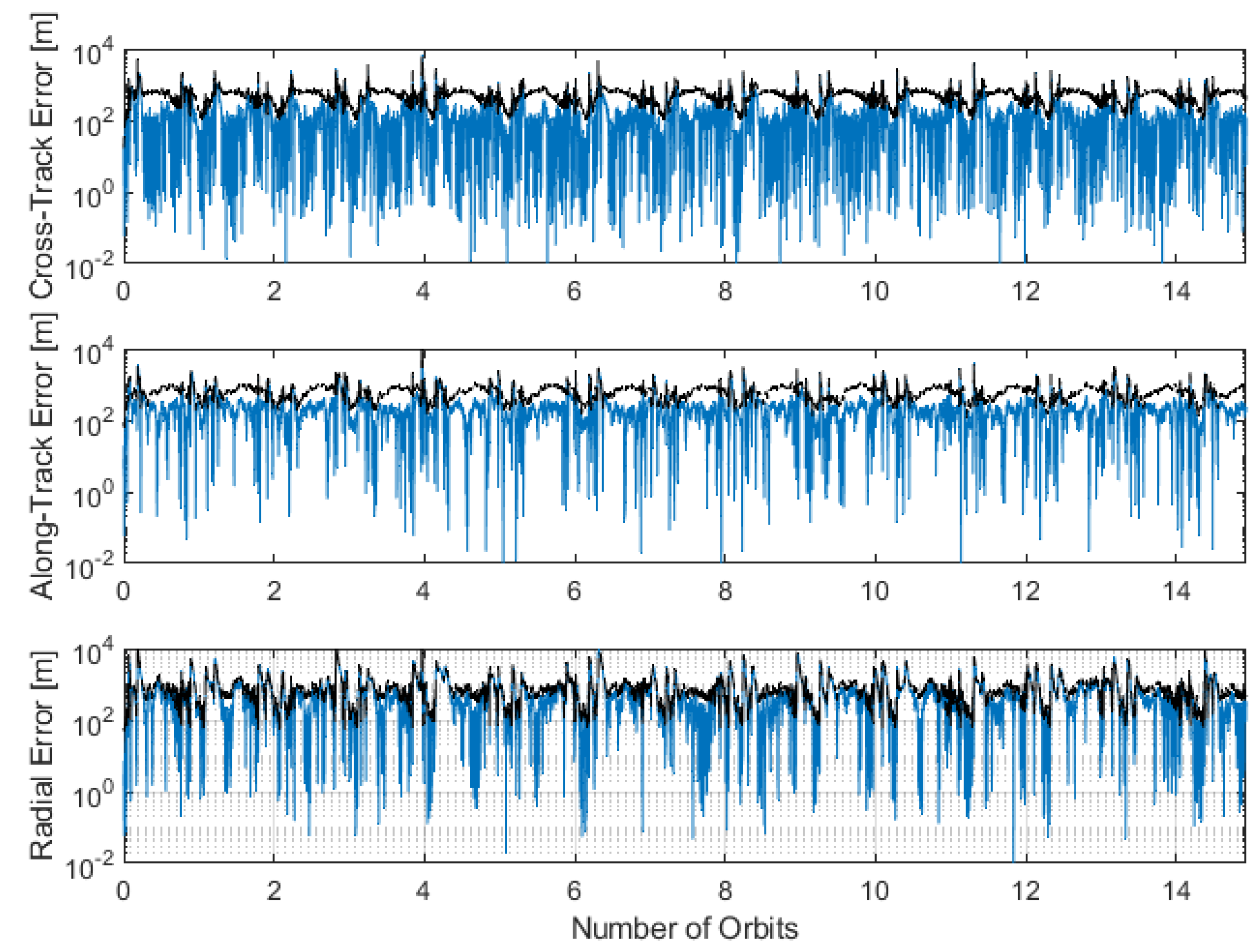
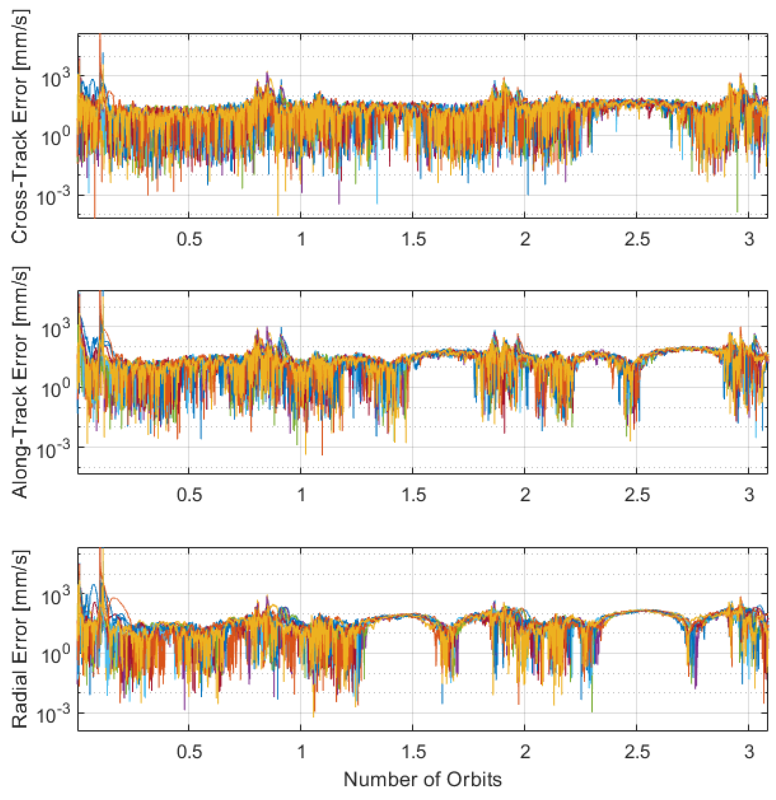
The ISL can support with performance, which is able to provide a relative measurement to the neighbouring satellite’s range and range-rate. This technique may only be used in combination with other celestial sensors, which provide an absolute position reference to the Moon. The performances of the EKF methodology are presented in Table 4 as an average of all ten satellites, alongside a plot of performance over time of the position and velocity errors in Figure 13 and Figure 14 respectively. A horizon-only approach is treated since it delivers the best performance in Table 3.
Table 4.
EKF for an ISL-assisted horizon-based optical navigation system at 1.
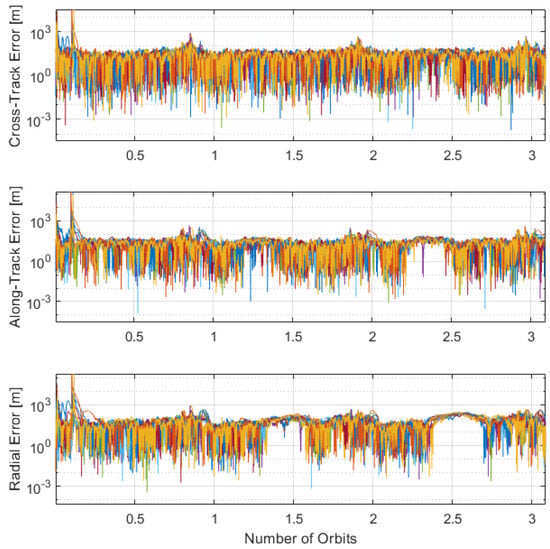
Figure 13.
Inter-satellite link with lunar horizon position error for 10 distributed spacecraft in ELFO.
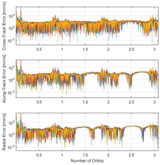
Figure 14.
Inter-satellite link with lunar horizon velocity error for 10 distributed spacecraft in ELFO.
However, the approach of using an ISL presents challenges to pointing, where it may not be possible for both a link to be maintained and a camera pointed towards the lunar limb. Times have been staggered in this model to cope with these challenges, with updates from 10–60 s from ISL and horizon sensors varying during operations.
The performances indicated by Table 4 show that with the addition of the ISL, the performance and solution stability improve to around 100 m. This may be sufficient to support orbit determination of an LCNS but does not meet the requirement of 30 m.
5. Conclusions
Various approaches to optical navigation are compared in this article to deliver a lunar-based positioning system. Lunar exploration roadmaps from space agencies such as NASA and JAXA seek surface positioning performances below 40 m. This is difficult if the orbit determination of the ranging satellites is not below 30 m.
Optical systems compared include lunar and Earth horizon-sensing systems, lunar craters, and celestial body triangulation by point sources. As stand-alone sources, they do not meet the performance requirements. The lunar limb approach presents the best possible performances.
The article then considers sensor fusion by optical approach and inter-satellite links. This may deliver a performance around 100 m that might be applicable to an LCNS. The filter stability is not constant, however, and so the required user performance may not be achieved at all times. Additional sensor measurement might be required, and will need further study. Some of these methods will be implemented and tested using the University of Tokyo EQUULEUS spacecraft, which has been recently launched with successful initial operations on-board Artemis I.
Author Contributions
Conceptualization, methodology, software, J.J.R.C.-M.; supervision, X.W.; conceptualization, methodology, Y.K.; supervision, project administration, S.N. All authors have read and agreed to the published version of the manuscript.
Funding
This research was partially funded by the NSW Space Research Network Grant Number SRN-Pilot-2022-04.
Data Availability Statement
Data are contained within the article.
Acknowledgments
The authors would like to thank The University of Tokyo for welcoming Joshua Critchley-Marrows as a visiting researcher in the Intelligent Space Systems Laboratory (Nakasuka-Funase Laboratory) from October 2022 to March 2023, therefore enabling this study.
Conflicts of Interest
The authors declare no conflicts of interest.
References
- Tripathi, S. It’s Going to Get Very Busy on the Moon; India Today: New Delhi, India, 2022. [Google Scholar]
- Skibba, R. Humans Are Revisiting the Moon—And the Rules of Spacefaring; Wired Magazine: New York, NY, USA, 2022. [Google Scholar]
- McKie, R. The Moon, Mars and Beyond… the Space Race in 2020. In The Observer; The Guardian: London, UK, 2020. [Google Scholar]
- Israel, D.J.; Mauldin, K.D.; Roberts, C.J.; Mitchell, J.W.; Pulkkinen, A.A.; Cooper, L.V.D.; Johnson, M.A.; Christe, S.D.; Gramling, C.J. LunaNet: A Flexible and Extensible Lunar Exploration Communications and Navigation Infrastructure. In Proceedings of the 2020 IEEE Aerospace Conference, Big Sky, MT, USA, 7–14 March 2020; pp. 1–14. [Google Scholar] [CrossRef]
- Giordano, P.; Grenier, A.; Zoccarato, P.; Bucci, L.; Cropp, A.; Swinden, R.; Gomez Otero, D.; El-Dali, W.; Carey, W.; Duvet, L.; et al. Moonlight navigation service—How to land on peaks of eternal light. In Proceedings of the 72nd International Astronautical Congress, Dubai, United Arab Emirates, 25–29 October 2021; pp. 1–14. [Google Scholar]
- Kakihara, K.; Shibukawa, T.; Takahashi, R.; Tsuji, M.; Chikazawa, T.; Suzuki, N.; Ichimura, S.; Nakahashi, S.; Shinbo, H.; Takahashi, T.; et al. Study on Lunar Communications and Navigation Architecture Utilizing Micro-Satellites. In Proceedings of the 66th Joint Conference on Space Science and Technology, Kumamoto, Japan, 8–10 November 2022; pp. 1–6. [Google Scholar]
- Ogino, K.; Kawabata, Y. Research on orbit optimization of lunar South Pole positioning by small satellites focusing on elliptical orbit. In Proceedings of the 66th 34th International Symposium on Space Technology and Science, Kurume, Japan, 3–9 June 2023; pp. 1–8. [Google Scholar]
- Kim, Y.R.; Song, Y.J.; Park, J.I.; Lee, D.; Bae, J.; Hong, S.; Kim, D.K.; Lee, S.R. Ground Tracking Support Condition Effect on Orbit Determination for Korea Pathfinder Lunar Orbiter (KPLO) in Lunar Orbit. J. Astron. Space Sci. 2020, 37, 237–247. [Google Scholar] [CrossRef]
- Iiyama, K.; Bhamidipati, S.; Gao, G. Precise Positioning and Timekeeping in Lunar Orbit via Terrestrial GPS Time-Differenced Carrier-Phase Measurements. In Proceedings of the 2023 International Technical Meeting of The Institute of Navigation, Long Beach, CA, USA, 24–26 January 2023; pp. 213–232. [Google Scholar] [CrossRef]
- Parker, J.J.K.; Dovis, F.; Anderson, B.; Ansalone, L.; Ashman, B.; Bauer, F.H.; D’Amore, G.; Facchinetti, C.; Fantinato, S.; Impresario, G.; et al. The Lunar GNSS Receiver Experiment (LuGRE). In Proceedings of the 2022 International Technical Meeting of the Institute of Navigation, Long Beach, CA, USA, 25–27 January 2022; pp. 420–437. [Google Scholar] [CrossRef]
- Christian, J.A. A Tutorial on Horizon-Based Optical Navigation and Attitude Determination with Space Imaging Systems. IEEE Access 2021, 9, 19819–19853. [Google Scholar] [CrossRef]
- Franzese, V.; Di Lizia, P.; Topputo, F. Autonomous Optical Navigation for LUMIO Mission. In Proceedings of the 2018 Space Flight Mechanics Meeting. American Institute of Aeronautics and Astronautics, 2018, AIAA SciTech Forum, Kissimmee, FL, USA, 8–12 January 2018; pp. 1–11. [Google Scholar] [CrossRef]
- Zanetti, R.; Crouse, B.; D’souza, C. Autonomous Optical Lunar Navigation. In Proceedings of the AAS Spaceflight Mechanic Conference, Savannah, GA, USA, 8–12 February 2009; pp. 1–3. [Google Scholar]
- Mortari, D.; D’Souza, C.; Zanetti, R. Image Processing of Illuminated Ellipsoid. J. Spacecr. Robot. 2016, 53, 448–456. [Google Scholar] [CrossRef]
- Critchley-Marrows, J.; Wu, X.; Cairns, I. Stellar Navigation on the Moon—A Compliment, Support and Back-up to Lunar Navigation. In Proceedings of the ION ITM 2022, Long Beach, CA, USA, 25–27 January 2022; pp. 616–631. [Google Scholar]
- Maass, B.; Woicke, S.; Oliveira, W.M.; Razgus, B.; Krüger, H. Crater Navigation System for Autonomous Precision Landing on the Moon. J. Guid. Control. Dyn. 2020, 43, 1414–1431. [Google Scholar] [CrossRef]
- Qi, D.; Oguri, K. Investigation on Autonomous Orbit Determination in Cislunar Space via GNSS and Horizon-based Measurements. In Proceedings of the AAS/AIAA Space Flight Mechanics Meeting, Orlando, FL, USA, 8–12 January 2023; pp. 1–20. [Google Scholar]
- Iiyama, K.; Kawabata, Y.; Funase, R. Autonomous and Decentralized Orbit Determination and Clock Offset Estimation of Lunar Navigation Satellites Using GPS Signals and Inter-satellite Ranging. In Proceedings of the ION GNSS+ 2021, St. Louis, MO, USA, 20–24 September2021; pp. 936–949. [Google Scholar]
- Hesar, S.G.; Parker, J.S.; Leonard, J.M.; McGranaghan, R.M.; Born, G.H. Lunar far side surface navigation using Linked Autonomous Interplanetary Satellite Orbit Navigation (LiAISON). Acta Astronaut. 2015, 117, 116–129. [Google Scholar] [CrossRef]
- Critchley-Marrows, J.; Kawabata, Y.; Ogino, K.; Nakasuka, S. Autonomous Orbit Determination for Lunar Satellite Infrastructure in View of Continuity and Assurance. In Proceedings of the International Symposium on Space Technology and Science, Kurume, Japan, 3–9 June 2023; pp. 1–8. [Google Scholar]
- Flahaut, J.; Carpenter, J.; Williams, J.P.; Anand, M.; Crawford, I.A.; van Westrenen, W.; Füri, E.; Xiao, L.; Zhao, S. Regions of interest (ROI) for future exploration missions to the lunar South Pole. Planet. Space Sci. 2020, 180, 104750. [Google Scholar] [CrossRef]
- Bender, T.E.; Gabhart, A.S.; Steffens, M.J.; Mavris, D.N. Defining and Parameterizing the Design Space for Cislunar PNT Architectures. In Proceedings of the AIAA SCITECH 2023 Forum. American Institute of Aeronautics and Astronautics, 2023, AIAA SciTech Forum, National Harbor, MA, USA, 23–27 January 2023; pp. 1504–1510. [Google Scholar] [CrossRef]
- Pasquale, A.; Zanotti, G.; Prinetto, J.; Ceresoli, M.; Lavagna, M. Cislunar distributed architectures for communication and navigation services of lunar assets. Acta Astronaut. 2022, 199, 345–354. [Google Scholar] [CrossRef]
- Pereira, F.; Reed, P.M.; Selva, D. Multi-Objective Design of a Lunar GNSS. NAVIGATION J. Inst. Navig. 2022, 69, navi.504. [Google Scholar] [CrossRef]
- Zanotti, G.; Ceresoli, M.; Pasquale, A.; Prinetto, J.; Lavagna, M. High performance lunar constellation for navigation services to Moon orbiting users. Adv. Space Res. 2023; in press. [Google Scholar] [CrossRef]
- Ely, T.A. Stable Constellations of Frozen Elliptical Inclined Lunar Orbits. JAnSc 2005, 53, 301–316. [Google Scholar] [CrossRef]
- A Standardized Lunar Coordinate System for the Lunar Reconnaissance Orbiter and Lunar Datasets; National Aeronautics and Space Administration (NASA): Moffett Field, CA, USA, 2008.
- Montenbruck, O.; Gill, E. Satellite Orbits–Models, Methods, Applications; Springer: Berlin, Germany, 2000. [Google Scholar]
- Markley, F.L.; Crassidis, J.L. Filtering for Attitude Estimation and Calibration. In Fundamentals of Spacecraft Attitude Determination and Control; Springer Science and Business Media: New York, NY, USA, 2014; pp. 235–343. [Google Scholar]
- Liebe, C.C. Accuracy performance of star trackers—A tutorial. IEEE Trans. Aerosp. Electron. Syst. 2002, 38, 587–599. [Google Scholar] [CrossRef]
- Critchley-Marrows, J.; Wu, X. Investigation into Star Tracker Algorithms using Smartphones with Application to High-Precision Pointing CubeSats. Trans. Jpn. Soc. Aeronaut. Space Sci. 2019, 17, 327–332. [Google Scholar] [CrossRef]
- Mortari, D.; Samaan, M.A.; Bruccoleri, C.; Junkins, J.L. The Pyramid star identification technique. Navig. J. Inst. Navig. 2004, 51, 171–183. [Google Scholar] [CrossRef]
- Brown, J.; Stubis, K.; Cahoy, K. TETRA: Star Identification with Hash Tables. In Proceedings of the 31st Annual AIAA/USU Conference on Small Satellites, Logan, UT, USA, 5–10 August 2017; pp. 1–12. [Google Scholar]
- Suntup, M.; Cairns, I.; Critchley-Marrows, J.; Wu, X.; Albertson, D.; Guinane, J.; Jarvis, B. Implementation of a WFOV Star Tracker in CubeSat and Small Satellite Attitude Determination Systems. In Proceedings of the 43rd COSPAR Scientific Assembly, Sydney, Australia, 28 January–2 February 2021; Volume 43, p. 59. [Google Scholar]
- Christian, J.A.; Benhacine, L.; Hikes, J.; D’Souza, C. Geometric Calibration of the Orion Optical Navigation Camera using Star Field Images. J. Astronaut. Sci. 2016, 63, 335–353. [Google Scholar] [CrossRef]
- Critchley-Marrows, J.J.R.; Wu, X.; Cairns, I.H. An architecture for a visual-based PNT alternative. Acta Astronaut. 2023, 210, 601–609. [Google Scholar] [CrossRef]
- Mortari, D.; Romoli, A. StarNav III: A three fields of view star tracker. IEEE Aerosp. Conf. Proc. 2002, 1, 47–57. [Google Scholar] [CrossRef]
- Lampkin, B.A.; Smith, D.W. A Hand-Held Sextant Qualified for Space Flight; Technical Report; NASA: Washington, DC, USA, 1968. [Google Scholar]
- Critchley-Marrows, J.; Mortari, D. Vision-based navigation in low Earth orbit—Using the stars and horizon as an alternative PNT. Adv. Space Res. 2023, 71, 4802–4813. [Google Scholar] [CrossRef]
- Christian, J.A. Accurate Planetary Limb Localization for Image-Based Spacecraft Navigation. Am. Inst. Aeronaut. Astronaut. 2017, 54, 708–730. [Google Scholar] [CrossRef]
- Henry, S.; Christian, J.A. Absolute Triangulation Algorithms for Space Exploration. J. Guid. Control. Dyn. 2023, 46, 21–46. [Google Scholar] [CrossRef]
- Poirot, J.L.; McWilliams, G.V. Navigation by Back Triangulation. IEEE Trans. Aerosp. Electron. Syst. 1976, AES-12, 270–274. [Google Scholar] [CrossRef]
- Cleaver, R.F.; Sothcott, P.; Robinson, F.J. An automatic radio triangulation system. Proc. IEE—Part B Electron. Commun. Eng. 1960, 107, 22–32. [Google Scholar] [CrossRef]
- Dempster, A. Dilution of precision in angle-of-arrival positioning systems. Electron. Lett. 2006, 42, 291–292. [Google Scholar] [CrossRef]
- Cheng, Y.; Ansar, A. Landmark Based Position Estimation for Pinpoint Landing on Mars. In Proceedings of the 2005 IEEE International Conference on Robotics and Automation, Barcelona, Spain, 18–22 April 2005; pp. 1573–1578. [Google Scholar] [CrossRef]
- Leroy, B.; Medioni, G.; Johnson, E.; Matthies, L. Crater detection for autonomous landing on asteroids. Image Vis. Comput. 2001, 19, 787–792. [Google Scholar] [CrossRef]
- Christian, J.A.; Derksen, H.; Watkins, R. Lunar Crater Identification in Digital Images. J. Astronaut. Sci. 2021, 68, 1056–1144. [Google Scholar] [CrossRef]
- Hanak, C.; Crain, T. Crater Identification Algorithm for the Lost in Low Lunar Orbit Scenario. In Proceedings of the 33rd Annual AAS Guidance and Control, Breckenridge, CO, USA, 29 January–3 February 2010; pp. 1–27. [Google Scholar]
- Clerc, S.; Spigai, M.; Simard-Bilodeau, V. A crater detection and identification algorithm for autonomous lunar landing. IFAC Proc. Vol. 2010, 43, 527–532. [Google Scholar] [CrossRef]
- Park, W.; Jung, Y.; Bang, H.; Ahn, J. Robust Crater Triangle Matching Algorithm for Planetary Landing Navigation. J. Guid. Control. Dyn. 2019, 42, 402–410. [Google Scholar] [CrossRef]
- Silvestrini, S.; Piccinin, M.; Zanotti, G.; Brandonisio, A.; Bloise, I.; Feruglio, L.; Lunghi, P.; Lavagna, M.; Varile, M. Optical navigation for Lunar landing based on Convolutional Neural Network crater detector. Aerosp. Sci. Technol. 2022, 123, 107503. [Google Scholar] [CrossRef]
- Losiak, A.; Wilhelms, D.E.; Byrne, C.J.; Thaisen, K.; Weider, S.Z.; Kohout, T.; O’Sulllivan, K.; Kring, D.A. A New Lunar Impact Crater Database. In Proceedings of the 40th Lunar and Planetary Science Conference, The Woodlands, TX, USA, 23–27 March 2009; pp. 1–8. [Google Scholar]
- Fitzgibbon, A.; Pilu, M.; Fisher, R.B. Direct least square fitting of ellipses. IEEE Trans. Pattern Anal. Mach. Intell. 1999, 21, 476–480. [Google Scholar] [CrossRef]
- Abusali, P.A.M.; Tapley, B.D.; Schutz, B.E. Autonomous Navigation of Global Positioning System Satellites Using Cross-Link Measurements. J. Guid. Control. Dyn. 1998, 21, 321–327. [Google Scholar] [CrossRef]
- Chaudhry, A.U.; Lamontagne, G.; Yanikomeroglu, H. Laser Intersatellite Link Range in Free-Space Optical Satellite Networks: Impact on Latency. IEEE Aerosp. Electron. Syst. Mag. 2023, 38, 4–13. [Google Scholar] [CrossRef]
- Zech, H.; Biller, P.; Heine, F.; Motzigemba, M. Optical intersatellite links for navigation constellations. In Proceedings of the International Conference on Space Optics—ICSO 2018, Khania, Greece, 9–12 October 2018; SPIE: Stockholm, Sweden, 2019; Volume 11180, pp. 370–379. [Google Scholar] [CrossRef]
- Qin, T.; Macdonald, M.; Qiao, D. Fully Decentralized Cooperative Navigation for Spacecraft Constellations. IEEE Trans. Aerosp. Electron. Syst. 2021, 57, 2383–2394. [Google Scholar] [CrossRef]
- Lidov, M.L. The evolution of orbits of artificial satellites of planets under the action of gravitational perturbations of external bodies. Planet. Space Sci. 1962, 9, 719–759. [Google Scholar] [CrossRef]
- Butcher, J.C. Numerical methods for ordinary differential equations in the 20th century. J. Comput. Appl. Math. 2000, 125, 1–29. [Google Scholar] [CrossRef]
- Kenneally, P.W.; Schaub, H. High Geometric Fidelity Solar Radiation Pressure Modeling usingGraphics Processing Unit. In Proceedings of the AAS/AIAA Spaceflight Mechanics Meeting, Napa Valley, CA, USA, 14–16 February 2016. [Google Scholar]
- di Stefano, I.; Cappuccio, P.; Iess, L. Precise Modeling of Non-Gravitational Accelerations of the Spacecraft BepiColombo During Cruise Phase. J. Spacecr. Rocket. 2023, 60, 1625–1638. [Google Scholar] [CrossRef]
- Pavlis, N.K.; Holmes, S.A.; Kenyon, S.C.; Factor, J.K. An Earth Gravitational Model to Degree 2160: EGM2008. In Proceedings of the General Assembly of the European Geosciences Union, Vienna, Austria, 13–18 April 2008. [Google Scholar]
- Lemoine, F.G.; Goossens, S.; Sabaka, T.J.; Nicholas, J.B.; Mazarico, E.; Rowlands, D.D.; Loomis, B.D.; Chinn, D.S.; Neumann, G.A.; Smith, D.E.; et al. GRGM900C: A degree 900 lunar gravity model from GRAIL primary and extended mission data. Geophys. Res. Lett. 2014, 41, 3382–3389. [Google Scholar] [CrossRef]
- Konopliv, A.S.; Asmar, S.W.; Carranza, E.; Sjogren, W.L.; Yuan, D.N. Recent Gravity Models as a Result of the Lunar Prospector Mission. Icarus 2001, 150, 1–18. [Google Scholar] [CrossRef]
- Montenbruck, O.; Ramos-Bosch, P. Precision real-time navigation of LEO satellites using global positioning system measurements. GPS Solut. 2008, 12, 187–198. [Google Scholar] [CrossRef]
- Lundberg, J.B.; Schutz, B.E. Recursion formulas of Legendre functions for use with nonsingular geopotential models. J. Guid. Control. Dyn. 1988, 11, 31–38. [Google Scholar] [CrossRef]
- Kalman, R.E. A new approach to linear filtering and prediction problems. J. Fluids Eng. Trans. ASME 1960, 82, 35–45. [Google Scholar] [CrossRef]
- Carlson, N. Federated square root filter for decentralized parallel processors. IEEE Trans. Aerosp. Electron. Syst. 1990, 26, 517–525. [Google Scholar] [CrossRef]
- Crassidis, J.L.; Markley, F.L. Unscented filtering for spacecraft attitude estimation. J. Guid. Control. Dyn. 2003, 26, 536–542. [Google Scholar] [CrossRef]


Disclaimer/Publisher’s Note: The statements, opinions and data contained in all publications are solely those of the individual author(s) and contributor(s) and not of MDPI and/or the editor(s). MDPI and/or the editor(s) disclaim responsibility for any injury to people or property resulting from any ideas, methods, instructions or products referred to in the content. |
© 2024 by the authors. Licensee MDPI, Basel, Switzerland. This article is an open access article distributed under the terms and conditions of the Creative Commons Attribution (CC BY) license (https://creativecommons.org/licenses/by/4.0/).