Abstract
This paper investigates the performance of the forthcoming lunar navigation satellite systems for estimating not only the position of an onboard receiver in a lunar inertial reference frame but also, and with a consistent accuracy, the relative position between two or more spacecraft in proximity. This could be the case of two spacecraft performing a rendezvous, of a lander released by an orbiter, or the case of the permanent relative navigation service for a formation of satellites around the Moon. The considered observables are the pseudorange and pseudorange-rate measurements provided by the upcoming lunar communication and navigation system (LCNS), expected to support lunar missions. A single-stage Kalman filter is implemented, and its performance is demonstrated through error statistics, which are then compared to what can be achieved with sequential filtering.
1. Introduction
Satellite formations have proven to be instrumental in various space missions, enabling collaborative data acquisition, improved mission robustness, and enhanced scientific investigations. With renewed interest in lunar exploration (ref. [1]), the deployment of satellite formations in lunar orbits (ref. [2]) can be of great interest for comprehensive lunar studies. However, precise navigation and coordination of satellites within these formations pose unique challenges due to the absence of full lunar GNSS systems and limited lunar orbiter capabilities.
The possibility of offering a navigation service similar to GPS or GALILEO navigation systems, even on a reduced scale and limited performance, has been recently carried out by many studies (ref. [3]). Both NASA and ESA, with the Moonlight mission concept (ref. [4]) are making rapid progress in the development of dedicated navigation satellite systems for the navigation of both lunar rovers and orbiters. The Moonlight initiative aims at the creation of lunar communications and navigation services (Lunar Communications and Navigation Services, LCNS) and related infrastructure.
As reported in ref. [5], the constellation dedicated to navigation could be selected among well-known orbit families, such as Walker orbits, elliptical lunar frozen orbits (ELFO), and Earth–Moon libration points orbits. The ELFO constellation offers high stability of the orbital parameters, suitable to cover pole area and low station-keeping budgets, and this is therefore the baseline solution in the current studies (ref. [6]).
Because of the reduced number of satellites of the constellation, the design of the constellation is optimized for specific missions and specific areas of interest, which are usually related to rovers and landers in the Moon south pole region. Limitations on the service offered in the wider lunar service volume will follow.
This paper investigates the possibility of extending the use of these navigation signals to the estimation of the relative state of a formation of two or more satellites in Moon orbit. In ref. [7] the problem was solved by implementing a cascade of filters approach: the first filter stage focused on estimating the position of each satellite of the formation in the Moon inertial frame, leveraging the pseudorange and pseudorange rate measurements, and accounting for the complex gravitational influences and perturbations encountered in the lunar environment. This first Extended Kalman Filter (EKF) can provide estimates that can be considered satisfactory for the individual satellite orbit determination but could prove insufficient when directly used to compute the relative state, with large percentage errors with respect to the formation baseline. A second filtering stage was therefore implemented, designed to estimate the relative position between satellites within the formation. By incorporating inter-satellite dynamics, this filter leverages the inertial position estimates of the first filtering stage to achieve a final relative state estimation that is less affected by the lack of a sufficient number of navigation signals, which periodically happens (because of the reduced number of navigation satellites). Notice that this architecture adds to the individual satellite navigation solutions that will still be available.
In the present research, a different approach, definitely oriented to formations, is investigated. A single-stage unscented Kalman filter (UKF) is developed taking inertial and relative dynamics into account; the process and measurement equations will be described, and the results will be presented. The larger computational cost of the UKF, which is required for handling the complexity of the measurement equations when the new state vector is considered, is rewarded by a greater accuracy, as will be shown with the comparison with the cascade filter of ref. [7]. The focus is particularly on relative navigation, so the estimates of relative orbital elements and relative position vectors are used to test the performance in a relative motion scenario that has been selected to be representative of a generic formation mission. The novelty of the paper does not lie in the filtering algorithms, as both EKF and UKF are well-known and established techniques. Instead, the paper investigates a new and relatively unexplored field—the application to the specific case of lunar formations that can leverage navigation satellite systems. Determining the optimal approach for relative configuration estimation remains an ongoing challenge, especially in this scenario, and this paper endeavors to provide essential data and performance indices to contribute to the definition of the navigation architecture.
The paper is organized as follows: Section 2 introduces the constellation of the navigation satellites; Section 3 describes the mission scenario; the cascade EKF is detailed in Section 4, while the novel single-stage UKF is described in Section 5. The comparison of the results of the two filtering architectures can be found in Section 6. Section 7 reports the final remarks.
2. Elliptical Lunar Frozen Orbit (ELFO) Constellation
The orbital parameters of the satellites of the candidate ELFO constellation for satellite navigation (ref. [8]) are selected to provide high stability, and significant coverage of pole areas (in particular the South pole) while requiring low station-keeping budgets and minimizing orbit maintenance costs.
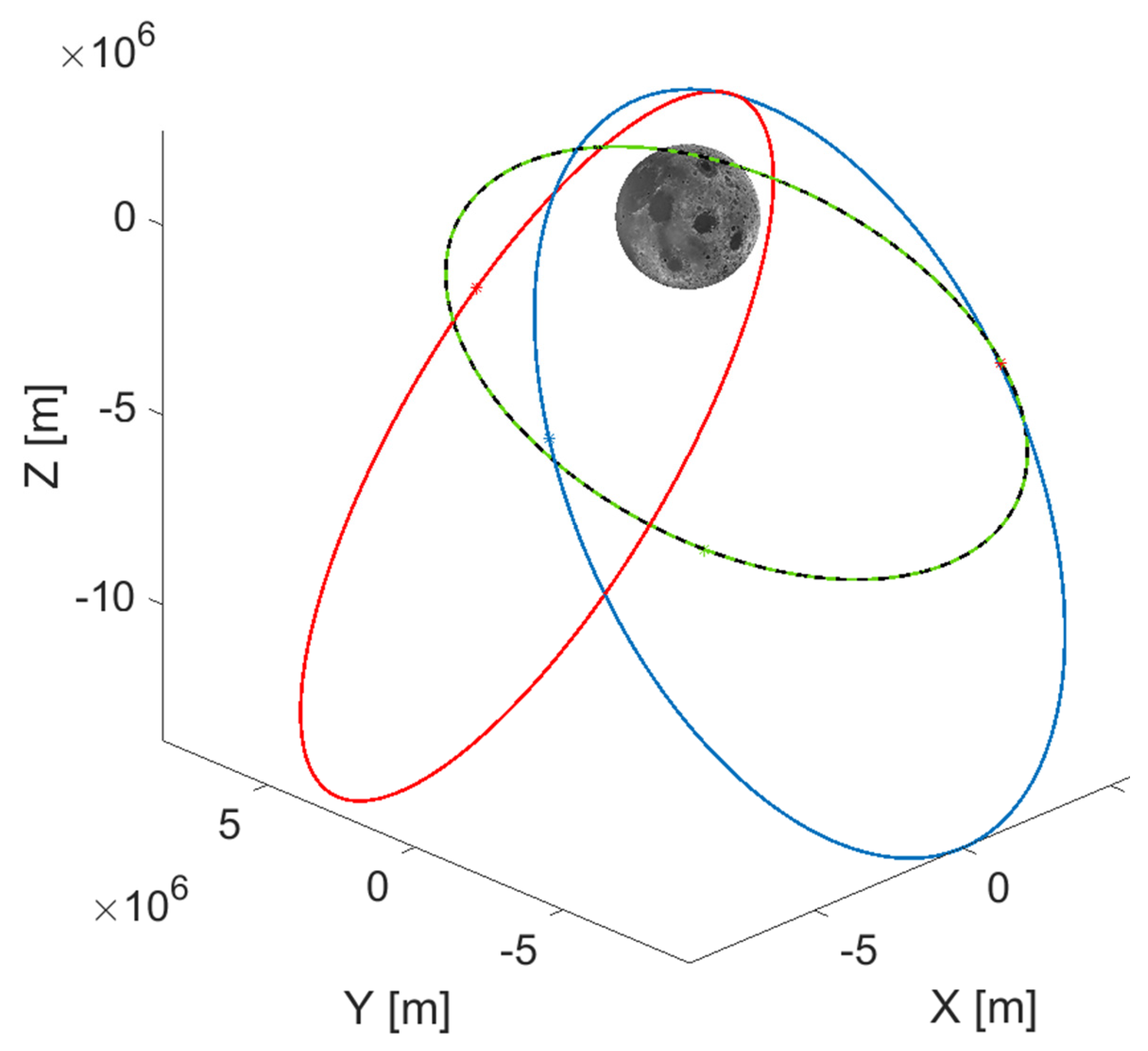
With respect to ref. [9] (where a constellation of 5 satellites was considered), in this work four ELFO satellites in three different orbital planes are considered (as in ref. [5]). This is a minimum for satellite navigation; thus, the performance obtained with this minimum configuration could only improve when larger constellations should be considered. The selected parameters are described in Table 1. and the resulting orbits are reported in Figure 1. The orbits are propagated in a Moon Inertial frame, centered in the Moon, is defined as an inertial system referenced to the Moon equator (at theJ2000 epoch) with x-axis pointing along the line formed by the intersection of the Moon equator and Earth’s mean equator at J2000. The z-axis points along the Moon’s spin axis direction at the J2000epoch. The y-axis completes the right-handed set.

Table 1.
Initial ELFO constellation parameters.
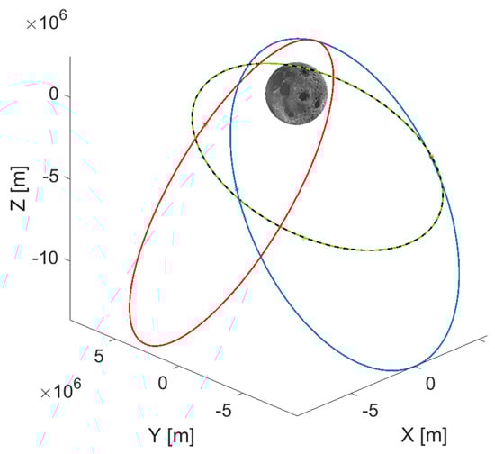
Figure 1.
3D representation of the ELFO constellation in the Moon Inertial reference frame. Notice the apolunes located above the southern hemisphere to best service in the southern polar cap. Blue, red, black and dotted green represents the orbits of the four ELFO satellites.
A simplified model is adopted for assessing the visibility of an ELFO satellite from a receiver, only relying on geometrical considerations. A navigation signal is considered received if:
- (a)
- The vector from the ELFO satellite to the receiver is not intercepted by the Moon (plus a 50 km mask altitude);
- (b)
- The vector from the ELFO satellite to the receiver is inside a 15-degree semi-aperture cone representing the transmitting antenna pattern. The current design of the LCNS platforms is similar to terrestrial GNSS and includes a radiation pattern focused on the nadir direction. Conservatively, the paper follows the same approach.
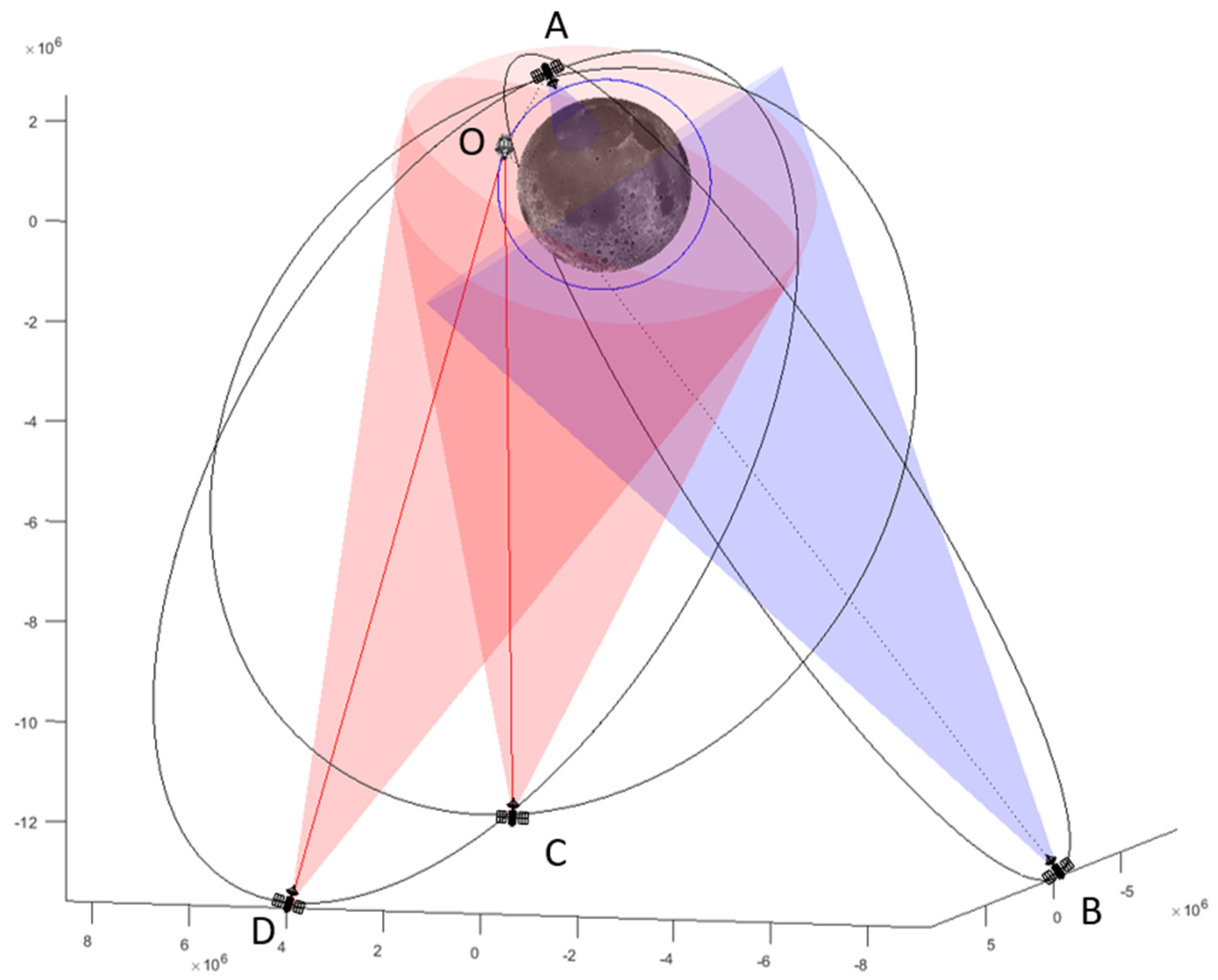
As an example, referring to Figure 2, orbiter O has visibility of ELFO satellites C and D (the vector from satellites to orbiter is inside the antenna main lobe), while it does not have visibility of satellites A (relative position vector outside the main lobe) and B (relative vector would be inside the lobe, but Moon body is between the orbiter and the satellite).
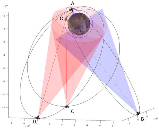
Figure 2.
Geometric visibility conditions. Red lines indicate a visibility condition, blue-dotted lines indicate a condition of non-visibility.
The number of visible satellites changes according to the orbital parameters of the receiver. As an example, it is possible to see from Figure 3 that the percentage of time in which full visibility (i.e., four satellites) is achieved, increases from equatorial to polar orbits. Quite interestingly, also the worst conditions (zero or just one visible satellite) increase from equatorial to polar orbits. This behavior depends on the fact that the LCNS constellation has been specifically designed for future missions to the Moon’s south pole, where the navigation performance is optimized.
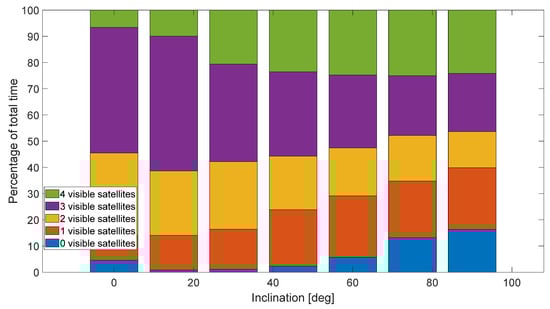
Figure 3.
Visibility conditions as a function of the orbit inclination.
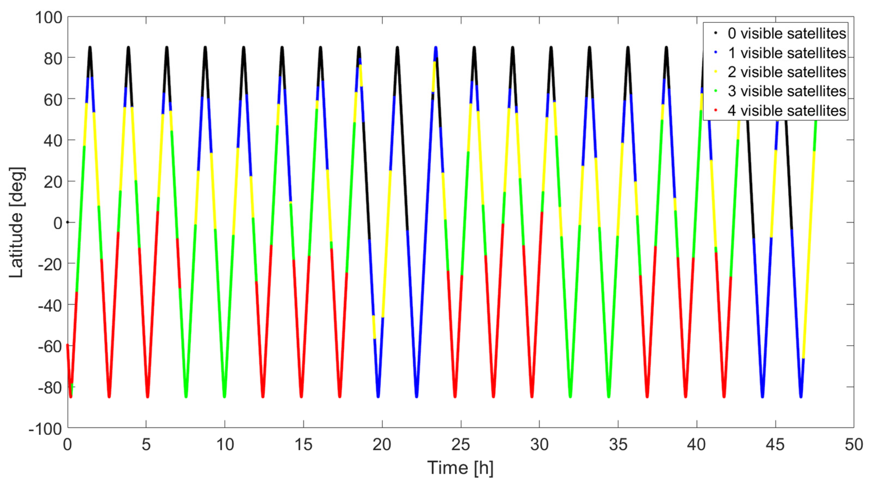
Confirmation can be obtained by looking at Figure 4. Here, the number of visible satellites is plotted as a function of the receiver latitude for a polar orbit case. The North Pole (90 degrees latitude) suffers from nearly null coverage, as opposed to the South Pole (−90 degrees), where most of the time there are three or four visible satellites. It can also be noticed that there is a 24 h periodic behavior in the visibility conditions.
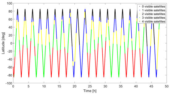
Figure 4.
Number of visible satellites as a function of the latitude for a polar orbiter.
Since the case of greater interest for future missions is the South Pole exploration, also the reference orbit of the formation of satellites is considered to be on a nearly polar orbit (which is therefore periodically affected by the worst and by the best visibility conditions). The analysis in Figure 5 shows that the visibility conditions for such a kind of orbital scenario are not affected by the right ascension of the ascending node (RAAN).
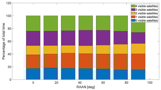
Figure 5.
Visibility conditions for a polar orbit, at different RAAN angles.
3. Mission Scenario
A formation of two satellites, called Chief (subscript C in the following) and Deputy (subscript D), is considered. The Chief satellite is orbiting on a circular polar orbit with the following orbital parameters in Table 2:
Table 2.
Chief satellite orbital parameters.
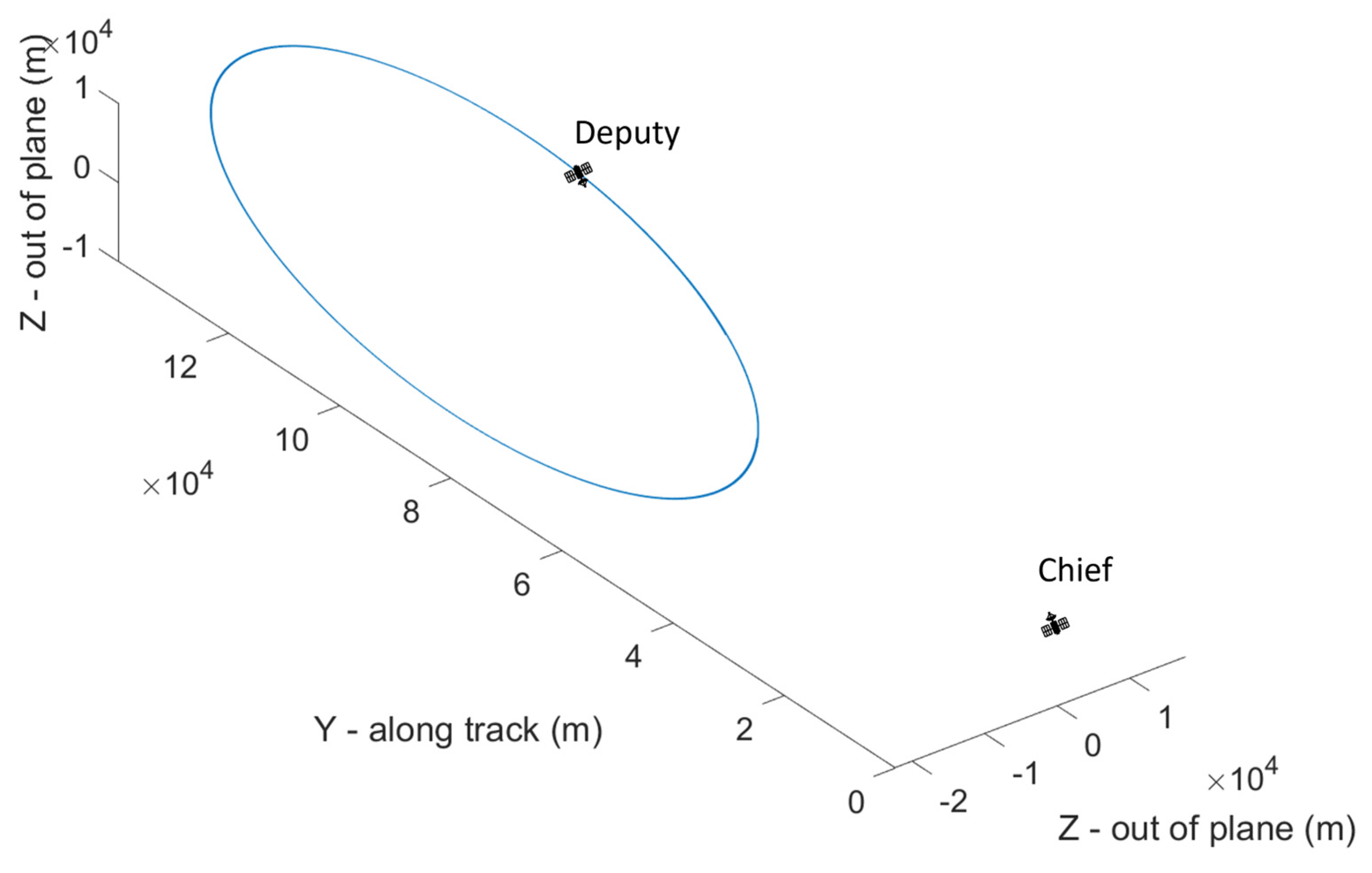
The Deputy orbit is selected in such a way that its relative motion with respect to the Chief includes most of the possible characteristics of the formation flying dynamics, so to provide more generality to the study. Specifically, an elliptical relative trajectory (semiaxes dimensions (20, 40, 20) km in the radial, along-track, and out-of-plane direction, respectively), with an along-track offset of 100 km, is considered. In Figure 6, the trajectory in the local vertical local horizontal (LVLH) reference frame is reported, where the x-axis is in the radial direction, the z-axis is out-of-plane, and the y-axis forms a right-handed frame.
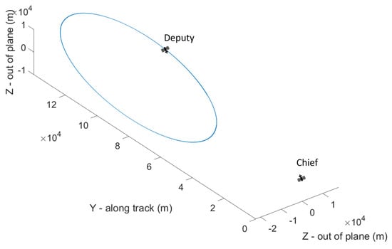
Figure 6.
Relative motion in the LVLH frame.
The orbital propagator for Chief and Deputy satellites includes the first 20 harmonics of the Moon’s gravitational potential, the gravitational attraction of the Earth and the Sun, and the solar radiation pressure (modeled as in ref. [10]).
4. Cascade Filter Approach
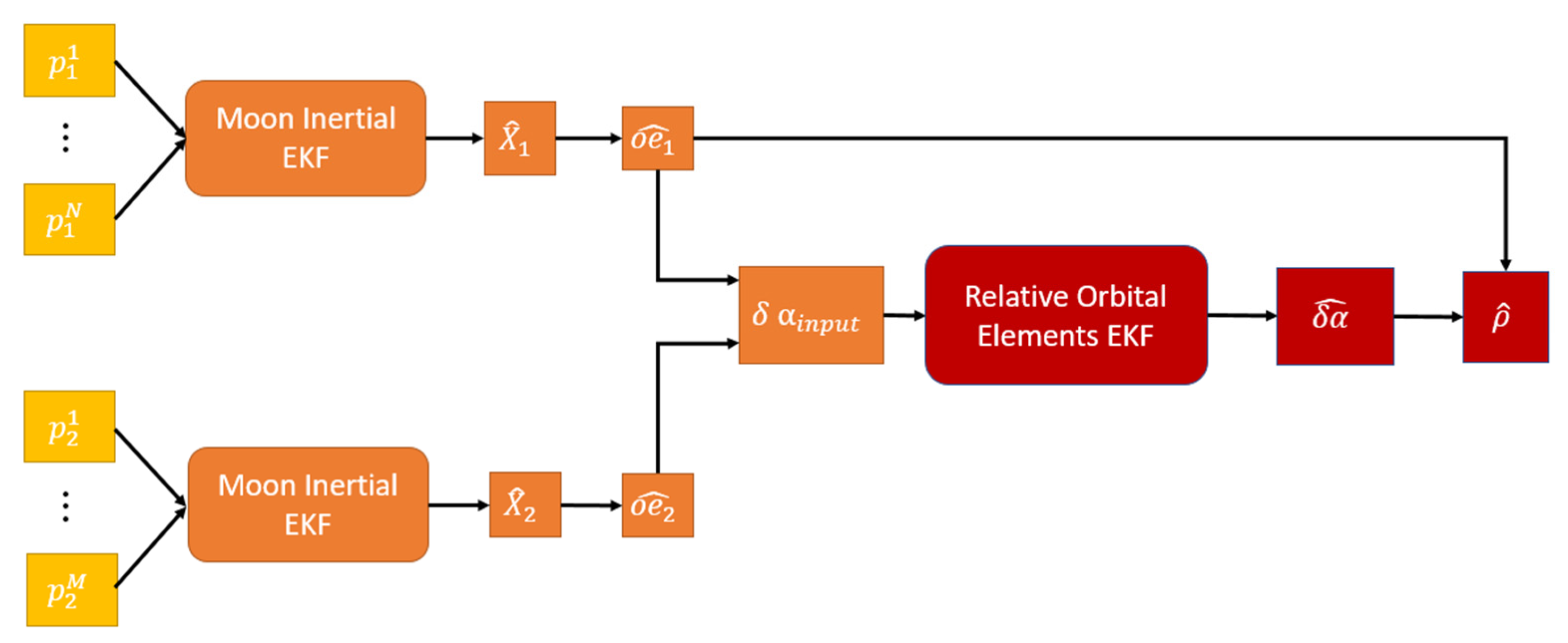
In ref. [11] an EKF for the estimation of the position and velocity of a satellite in a Moon inertial frame was presented. Even though it was demonstrated that the performance achieved is satisfactory even when very few ELFO satellites are in visibility (the reader can refer to following Section 6.1 for an example of the performance of the absolute navigation), the accuracy obtained by applying the same filter to the Chief and Deputy and simply differencing the estimates is not an advisable procedure if the focus is on the relative motion, i.e., on the estimation of the relative dynamics. Therefore, the problem was faced in ref. [7] by implementing a cascade filter architecture, in which the input to the second stage of the filter (dedicated to relative state estimation) is the output of the first stage filters (estimating the position of the two satellites in the Moon inertial frame), as shown in Figure 7. A brief explanation of this filter is reported in the following paragraphs since some concepts will be re-used for the newly developed filter that is the main objective of this research.

Figure 7.
Cascade filter architecture implemented for relative state estimation.
4.1. Moon Inertial State Estimation
As recalled in ref. [8], lunar navigation satellite system ranging code and navigation messages will be broadcasted by the satellites and exploited by the user to compute its own position. In this way, the user receiver could exploit all the already tested and robust GNSS receiver approaches to compute its own position.
As well known, at least four satellites would be necessary to algebraically compute the receiver position (and associated clock delay). In a lunar system made of just four satellites, the time availability of all satellites is quite limited and calls for an estimation of the state to extend the navigation also when availability is much lower. At the scope, a filter can be developed, which is however not the main interest of the study; it will be briefly explained, while its performance and limitations, together with its possible improvements are left to parallel publications (ref. [11]).
As explained shortly after, the measurement equations are nonlinear, and therefore an Extended Kalman Filter (EKF) will be implemented. For each tracked satellite, the usual steps of EKF are performed (ref. [12]), as follows:
- (a)
- Initialization;
- (b)
- Propagation;
- (c)
- Kalman gain computation;
- (d)
- Update.
The use of Kalman filters, in the extended form or modified implementations is a common approach as documented for example in refs. [13,14] and in the survey [15]. The state to be estimated is formed by the receiver state (position and velocity in the Moon inertial frame) and the receiver clock error, defined as a clock bias, c0, and a clock drift c1.
Here and in the following hat (^) symbol stands for estimated quantities, while tilde (~) symbol stands for predicted quantities. In the propagation phase both the state and the associated error covariance matrix P are propagated over a time step DT, starting from a previous estimate, and respectively.
The dynamics equations used for the propagation of the satellite state is provided by the orbital dynamics of a body orbiting the Moon:
where finer(X,t) is represented by the same dynamic model used for the propagation. The more accurate the dynamics, the lower can be the so-called process error or . At the same time, the larger is the computation time. This, however, is true only when there is full visibility of the LCNS satellites. In fact, the influence of the error of the last estimated position and velocity values during full visibility phases will have a larger impact on successive estimates’ errors if there is too-high trust in the propagated state (i.e., too low values of ). Therefore, a trade-off analysis must be implemented to balance between low values of (causing very good estimates with full visibility but large divergence in poor visibility conditions) and large values of (noisy estimates in full visibility but reduced drift in poor visibility). The matrix used in the following simulations is a diagonal matrix:
where the diagonal terms optimized with a trial-and-error approach are here reported:
Notice that, together with the state, also the associated covariance matrix P must be propagated; a transition matrix is required, where the linearized state matrix must be numerically computed at each time step, further increasing the computation cost.
The measurements are the usual quantities of GNSS: pseudoranges and pseudorange rates , which are a nonlinear function of the state :
where is the difference between the satellite and the receiver position vectors; is the difference between the satellite and the receiver velocity vectors; is the clock error modelled with a linear model: , where is the clock bias and is the clock error drift. Finally, are the pseudorange and pseudorange rate noises, modelled as random Gaussian noise with standard deviation equal to 15 m and 0.15 m/s, respectively.
The measurement equation in Equation (4) can be used to compute the predicted measurements . A linearization of the measurement equation is needed for the computation of the Kalman gain. The dimensions of the measurement matrix Hk is 2Nsat × 8, where Nsat is the number of ELFO satellites visible at time tk (ranging from 1 to a maximum of 4). If no navigation satellite is in visibility, it means that no measurement is available, so the update phase is not carried out at the specific time step and the estimate coincides with the propagated state. In all other cases, each 2 × 8 block of Hk reads as:
where are the director cosine of the vector from the satellite s to the receiver, and (and analogous for Y and Z components). This matrix Hk is used to compute the Kalman gain:
which is then introduced in the updated equations, for computing the estimate:
4.2. Relative Motion
It is supposed that a communication link is available between Chief and Deputy, so that the information of the estimated position in the Moon inertial frame, as computed in Section 4.1, can be shared. In real applications, this inter-satellite link introduces a time delay, which is however neglected in this phase of the study. As soon as the inertial position of the two satellites is available, the relative state (in the LVLH frame) can be algebraically computed as follows.
Given the position of the two satellites of the formation, and the orbital parameters of the Chief, the relative position can be computed as:
The estimation procedure in Section 4.1 is run at each time step for the two satellites independently. The resulting estimates, , are computed, together with the (estimated) orbital parameters . It is possible to directly compute the (estimated) relative distance and compare the results with the true relative distance. In ref. [7] it is shown that, as for the single satellite case, also the relative state suffers from large periodical peaks of errors, which happen when a small number (or even none) of ELFO satellites is in visibility.
A Kalman filter is therefore implemented also for the relative dynamics estimation to improve the performance in the relative state estimation. The fundamental steps are formally the same as in the previous paragraph, but of course with different dynamics models and measurement equations.
There are several ways to model the relative motions of two spacecraft; relative coordinates in the LVLH frame are certainly one of the most intuitive and they allow for an immediate comprehension of the motion. However, dynamics models based on cartesian coordinates suffer from linearization (refs. [16,17]) or they become hard to model when perturbations are included; additionally, the coordinates are by nature varying with the orbital period. When relative orbital parameters are used, instead, their behavior is nearly constant and perturbations are much easier to include they do not suffer from linearization, but they provide information that does not immediately allow for the interpretation of the motion.
Therefore, the set of differential orbital parameters described in ref. [18] is used as a relative state to be estimated, defined as:
While for visualization purposes they are transformed in relative coordinates. For simplicity, all the differential perturbations (third body attraction, higher harmonics of the Moon gravitational potential, solar radiation pressure) are neglected in this formulation, therefore the resulting dynamics simply reads as:
Being μ the Moon gravitational parameter. The dynamics model is a nonlinear function of the differential semimajor axis, and for short distances (qualitatively below 100 km), also the linearized version can be used:
The input of the filter cannot be properly called measurements, since they are a mathematical manipulation of the estimates of the navigation system of the two satellites:
While the covariance matrix associated to the noise on the original measurements is clearly related to the noise of the pseudoranges and pseudorange rates, the covariance matrix of the input of the relative dynamics filter, zrel, is not straightforward. In fact, it depends on the error in the estimates of the first two filters in a highly nonlinear way. To compute at each timestep the value of the covariance matrix associated with the error of , indicated as , an unscented transformation is applied (ref. [19,20]); see ref. [7] for more details.
5. A Single-Stage UKF Filter for Formation Flying Lunar Navigation
The concept guiding the development of a new estimation strategy is that the inclusion of the relative dynamics information (which is the real focus of the algorithm) in the first (and unique) stage of the filter, greatly helps the relative state estimation. In the cascade filter, the random noise affecting the pseudoranges produces independent state estimates of the Chief and Deputy’s state vectors (first stage), and the errors affecting these two estimates are input to the second stage of the filter. In the unified filter approach, instead, the relative state is estimated taking directly the pseudoranges measurements into account, thus the measurement prediction in the filter is influenced by the fact that the relative orbital elements are mostly constant. The drawback of this approach is that the high nonlinearity of the relation between pseudorages (and pseudorange rates) and relative orbital elements suggest the implementation of an Unscented Kalman Filter (UKF), which is more computationally expensive. The use of UKF for orbit determination is not uncommon in literature, as can be seen for example in ref. [21].
The state vector for the single-stage UKF consists of the Chief’s state in the inertial frame and of the relative orbital elements:
The measurements are all the pseudorages and pseudorange rates received by the Chief and Deputy satellites (not necessarily from the same LCNS source). The relative position in the LVLH can be computed from the estimated vector, as in the scheme of Figure 8.
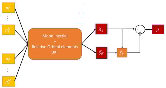
Figure 8.
The architecture of the single-stage UKF for formation navigation.
The implementation of the UKF requires a different way to compute the propagated state and the predicted measurement with respect to the EKF. Specifically, the following steps must be implemented (19):
- (1)
- From the state error covariance matrix, , and the previous estimate, , compute the 2n sigma points (being n the dimension of the state vector):
With:
Here indicates the i-th row of
- (2)
- Propagate the sigma points:where contains both the inertial dynamics of the Chief and the relative dynamics.
- (3)
- Compute the a priori state estimate by taking the arithmetic mean of the 2n sigma points . The a priori error covariance matrix is also obtained by the sigma points:
In the previous expression, the process matrix is a 14 × 14 matrix relevant to the position, velocity, and clock error dynamics, as in the EKF described in Section 4.1, and to the six relative orbital elements’ dynamics. Following similar considerations about the effect of tuning the matrix, we selected the process error matrix as a diagonal matrix with elements:
where the values of are the same used in Section 4.1, while is a six elements vector with all elements equal to
- (4)
- Predict the measurements. With a similar procedure to that of Equation (15), 2n sigma points are generated using the propagated state and relevant covariance matrix, . The measurement equation is then used to predict the measurements from the sigma points:
The measurement equation is made of two parts:
The second block of the measurement equations is highly nonlinear, and it consists in computing the inertial state of the Deputy, from , and , and applying . This requires transforming the inertial state in the orbital elements vector, then summing the the Deputy’ orbital elements are obtained; finally, the Deputy inertial state can be computed.
The predicted measurement vector is computed as the arithmetic mean of the vectors, and the estimated covariance of the predicted measurement, , and the cross covariance between prediction of the state and of the measurement, , are computed respectively as:
The Kalman gain can be now computed, and the new estimate is obtained:
6. Results
6.1. Cold Start
In this first simulation, the performance in terms of positioning error of the estimate is analyzed starting from the following initial errors:
where randn indicates a Gaussian random distribution of variance equal to one, while E0 is the initial error on the state (assumed equal to 10 km on each axis for the position, 100 m/s on each axis for velocity, 1 km for clock bias and 0.1 m/s for clock error drift). For the relative orbital element vector, the zero state has been selected as a reasonable initial guess. A Monte Carlo approach has been implemented, by running 100 simulations with random initial conditions and pseudorange noise, both for the single-stage UKF and the cascade EKF.
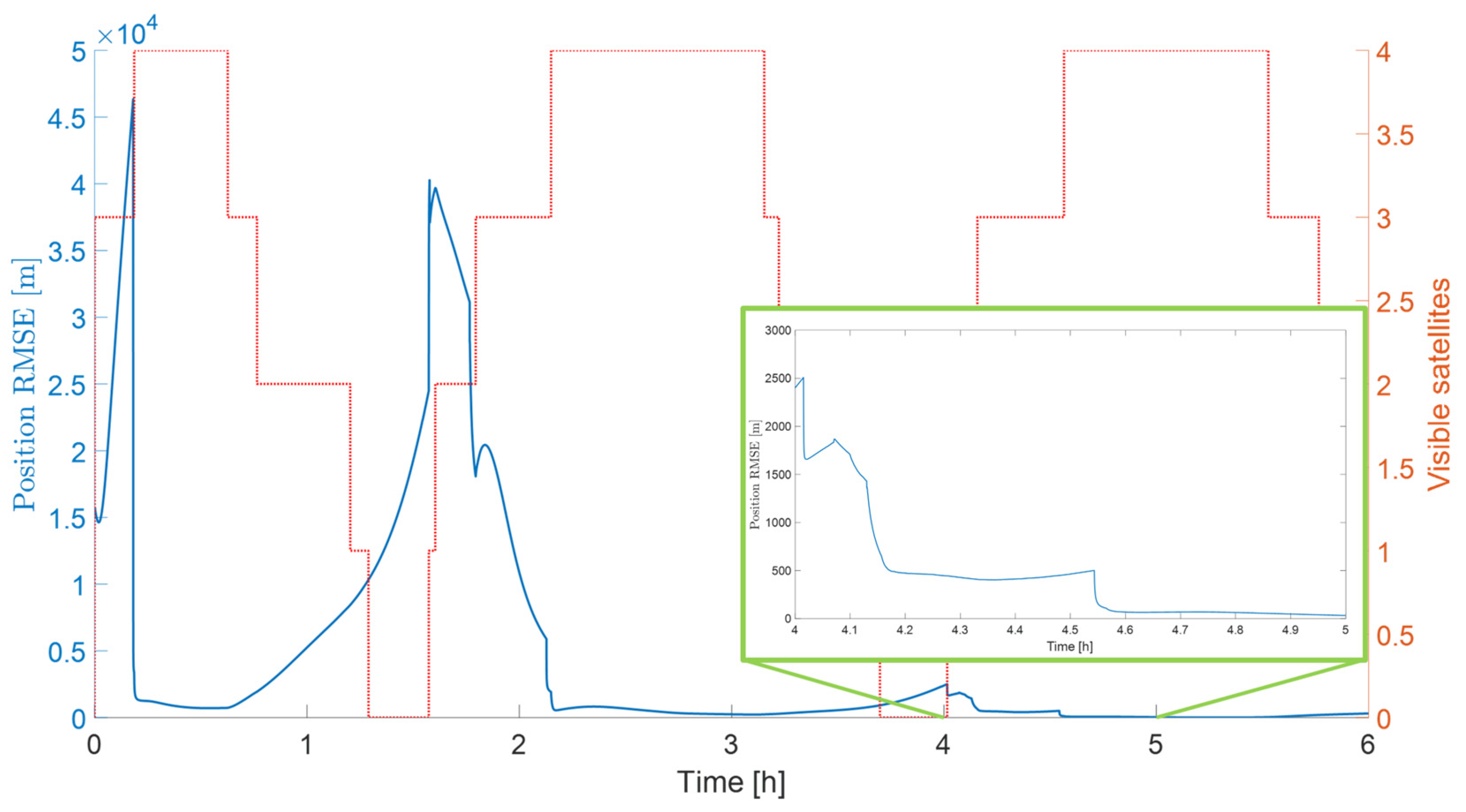
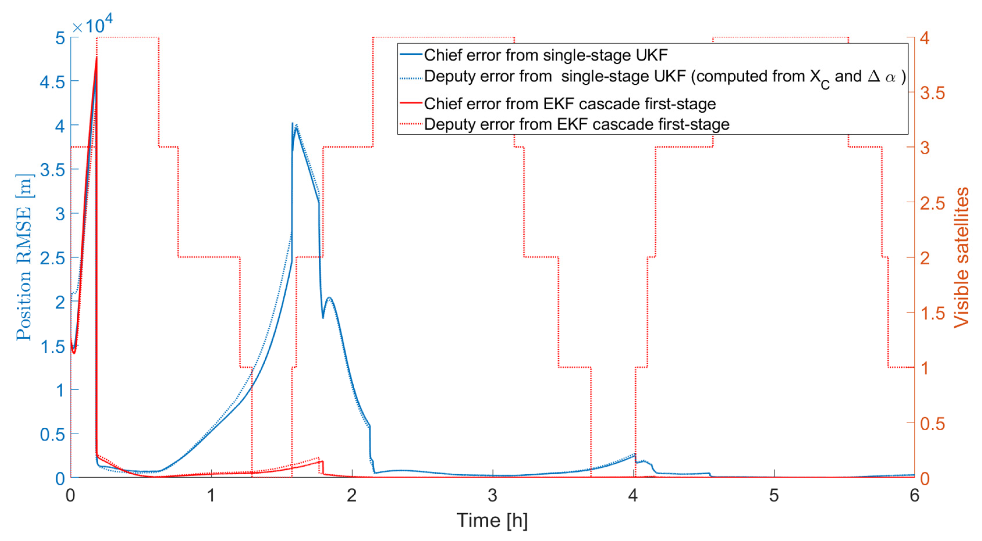
The time needed for achieving convergence mainly depends on the initial true anomaly of the ELFO satellites, allowing (or not) a full availability of the constellation in a short time. In Figure 9, the position error (obtained as the mean of the errors resulting from the Monte Carlo campaign) is plotted. It is possible to see that it is of the order of tens of kilometers for long latencies in availability, showing that the implemented UKF cannot converge if too few ELFO satellites are in visibility. The estimated error quickly improves when more satellites become available, ending with a very good accuracy after initialization, as depicted in the zoom-in Figure 9, with errors below 50 m. The convergence time is of the order of 4 h.
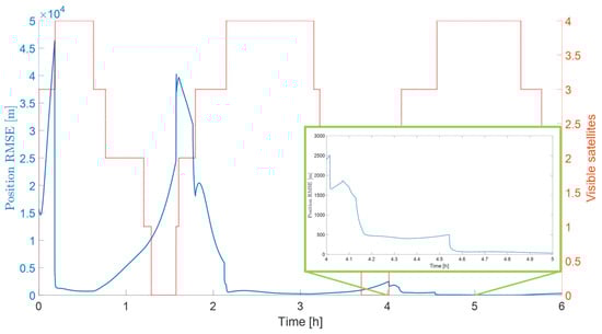
Figure 9.
Convergence of the single-stage UKF in the case of a cold start: Chief inertial state error norm. Blue line indicates the position RMSE, red line is the number of visible satellites.
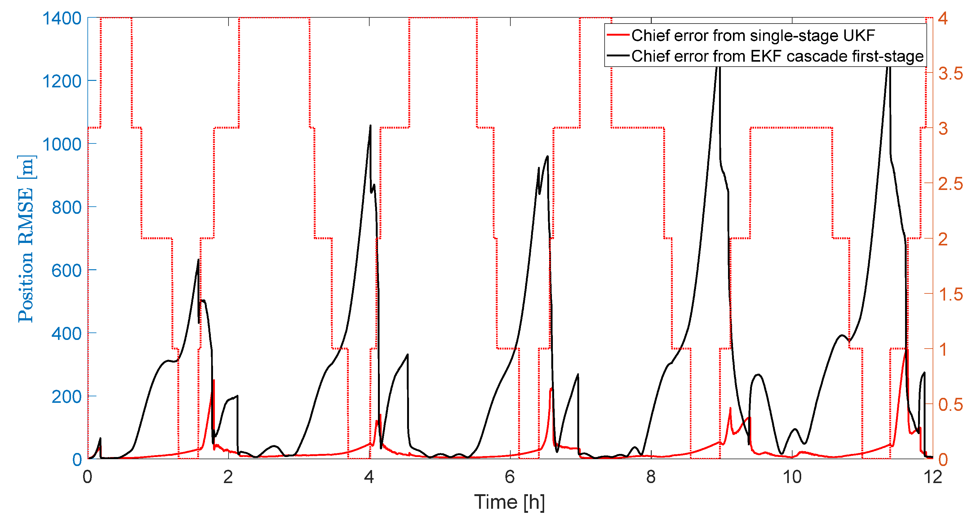
As a byproduct, also the inertial state of the Deputy (from the estimate of the inertial state of the Chief and the estimates of the relative orbital elements) can be computed, showing a very similar behavior. For comparison, the estimated position error norm of the Chief and Deputy obtained as the output of the first stage of the cascade filter is reported in Figure 10. Also in this case, the plotted curves are the result of the average of the results obtained by the two Monte Carlo campaigns (for the UKF and EKF cases). It is possible to see that the convergence is faster (about 2 h). However, the better performance on the inertial state of the two satellites does not produce a faster convergence in terms of relative orbital elements, which is the main objective of the current study.
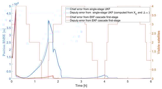
Figure 10.
Convergence time comparison of the inertial state using the cascade EKF and the single-stage UKF.
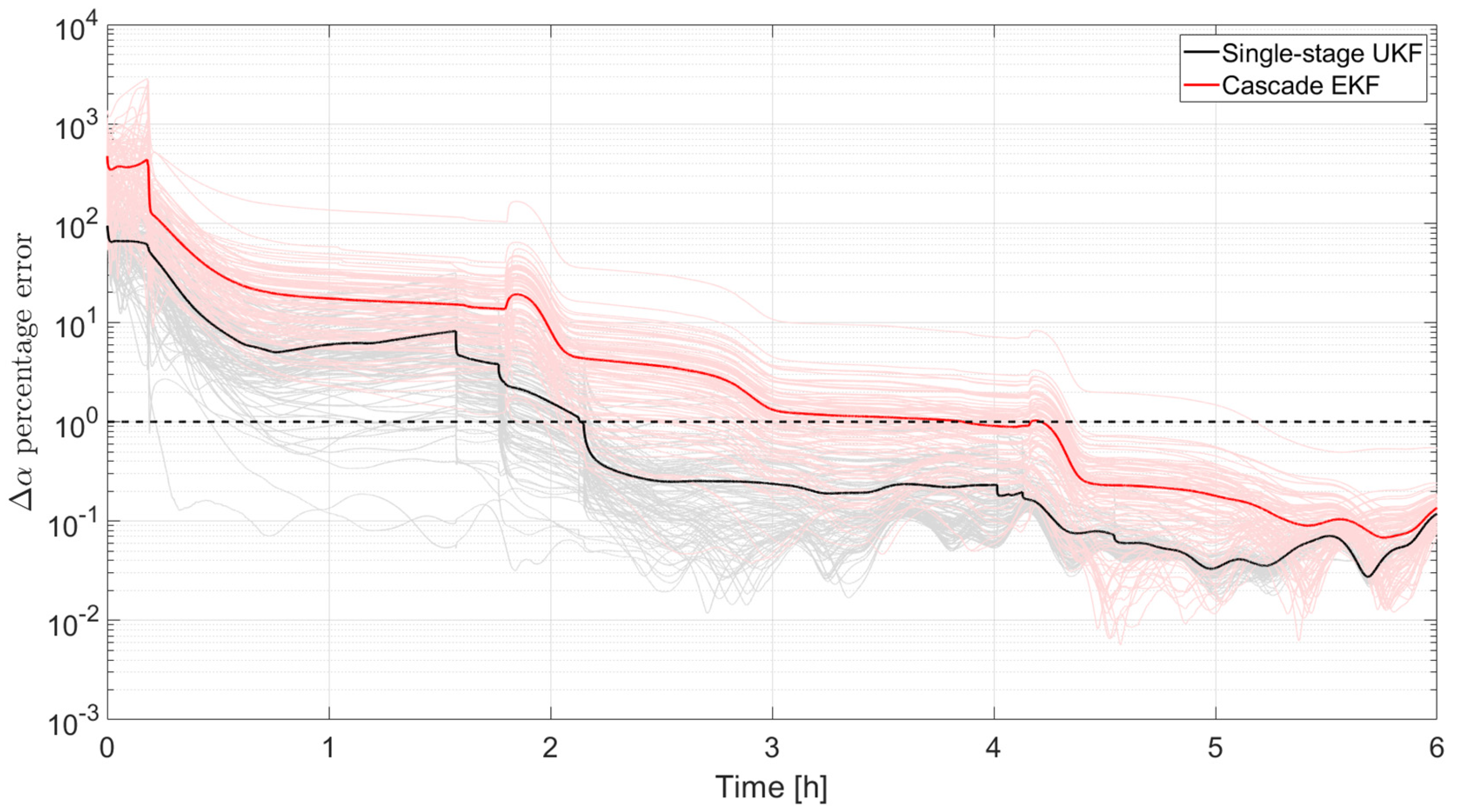
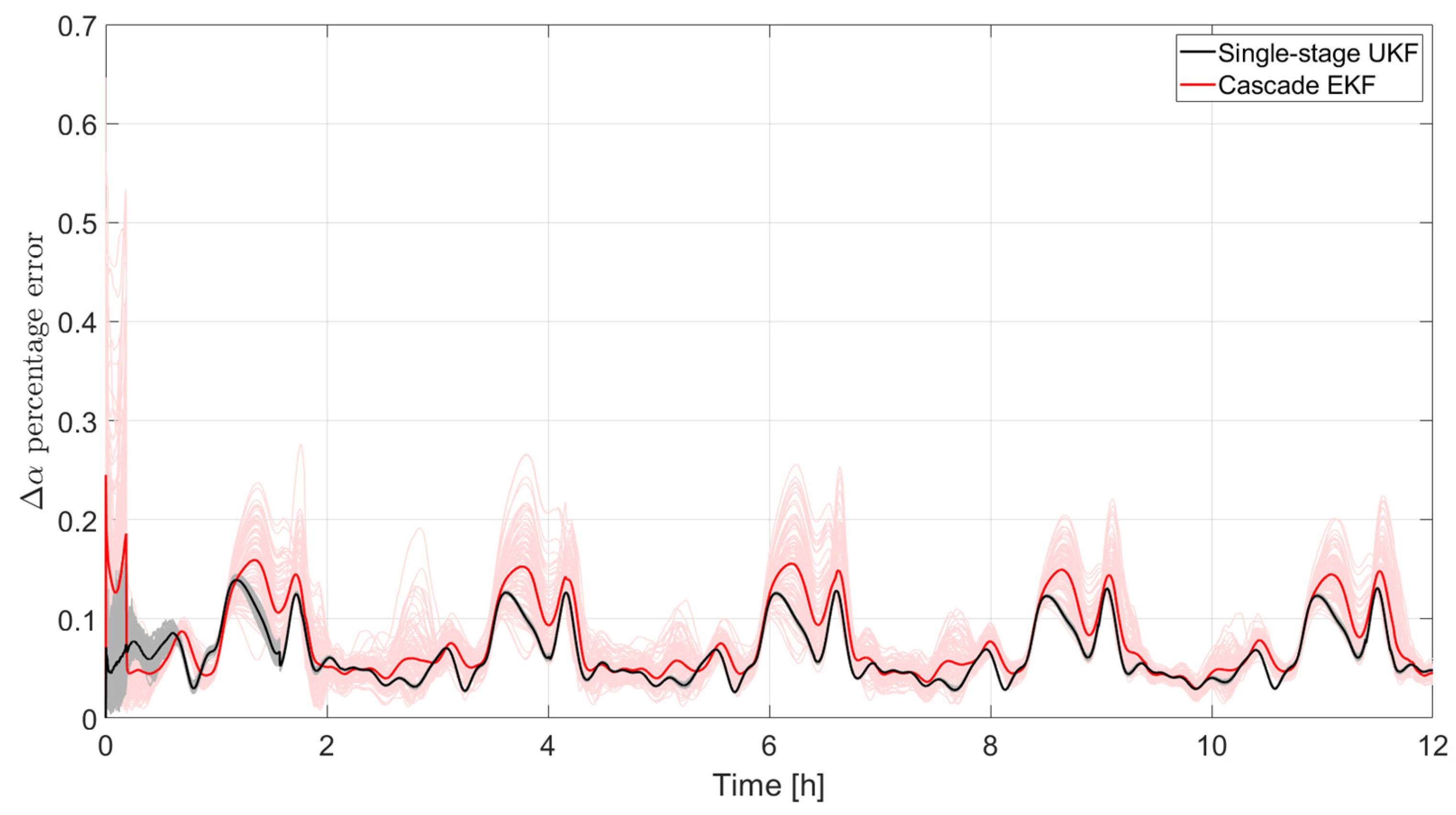
In Figure 11, the percentage of the error norm on the vector of the relative state vector is plotted for all the results obtained in the two Monte Carlo campaigns. The cascade EKF results are plotted in light red (with a bold red curve for the average value) while the single-stage results are plotted in a light curve (with a bold black curve for the average value). Considering the converge time as the time when the errors are consistently below the 1% value, it is possible to appreciate how the single-stage UKF converges much faster (approximately half of the time) than the cascade EKF.
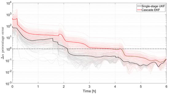
Figure 11.
Convergence of the single-stage UKF and the cascade EKF in the case of a cold start: relative orbital elements error norm.
6.2. Performance at Stationary
Since the initial large errors hide the behavior at stationary, in this paragraph the simulation is run with a perfect knowledge of the initial state.
As for the cold start case, a Monte Carlo approach is implemented for testing the performance of both the cascade EKF and the single-stage UKF, with randomly varying pseudorange noise signals. The accuracy in the estimates of the Chief and Deputy state computed at the first stage of the filter is better than what is achievable with the single-stage UKF (at least for the selected filter parameters that must be tuned in both filtering architectures), as reported in Figure 12, where the averaged values resulting from the Monte Carlo campaign are plotted. This is not an unexpected result: the Chief position is estimated in the first stage of the cascade EKF using a very accurate model of the Moon orbital dynamics. The same model is used in the single-stage UKF, but in that case, it is paired with a simplified model of the relative motion (in which all perturbations are neglected). The simplified relative dynamics model affects not only the relative state estimate but the state vector as a whole, including the inertial state of the Chief. Future development of the filter can include an improved version of the relative motion dynamics, but it is important to notice that the goal of the single-stage UKF is estimating the relative dynamics and not the inertial quantities. Therefore, the actual performance index that must be evaluated is the accuracy of the estimates of relative state.
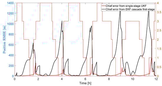
Figure 12.
Estimate the error norm of the Chief inertial position using the cascade EKF and the single-stage UKF.
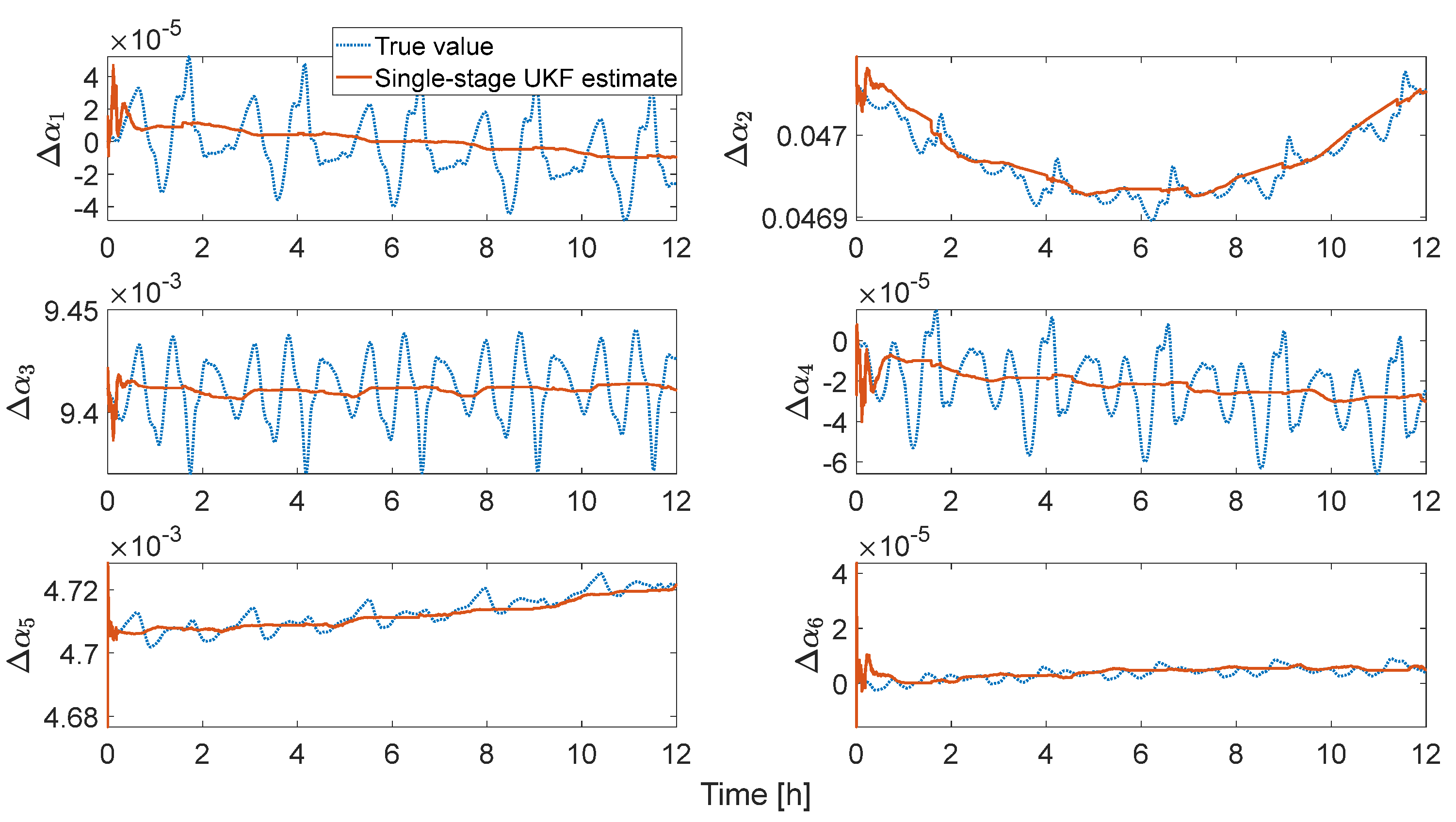
Figure 13 shows the true and estimated components of the vector obtained with the single-stage UKF. The presence of the gravitational and third-body perturbation produces oscillations in the values of the relative orbital elements, which the UKF is not able to capture. In fact, for simplicity, the relative dynamics is modeled as Keplerian. However, the lost information is of limited magnitude, as reported in Figure 14, where the percentage of the error norm on the vector of the relative state vector is plotted for all the results obtained in the two Monte Carlo campaigns; the color notation follows what indicated for Figure 11. It can be seen that the percentage errors are below 0.2% for both the single-stage UKF and the cascade EKF; however, the latter suffers from a much larger variability related to the random pseudorange noise, with errors that in the worst case reach 0.5%, more than double than the single-stage UKF.
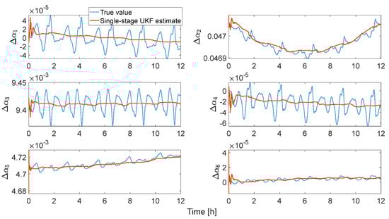
Figure 13.
Time behavior of the true and estimated relative orbital elements.
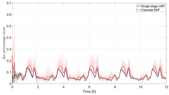
Figure 14.
Percentage difference between the norm of the true and of the estimated relative orbital elements vector.
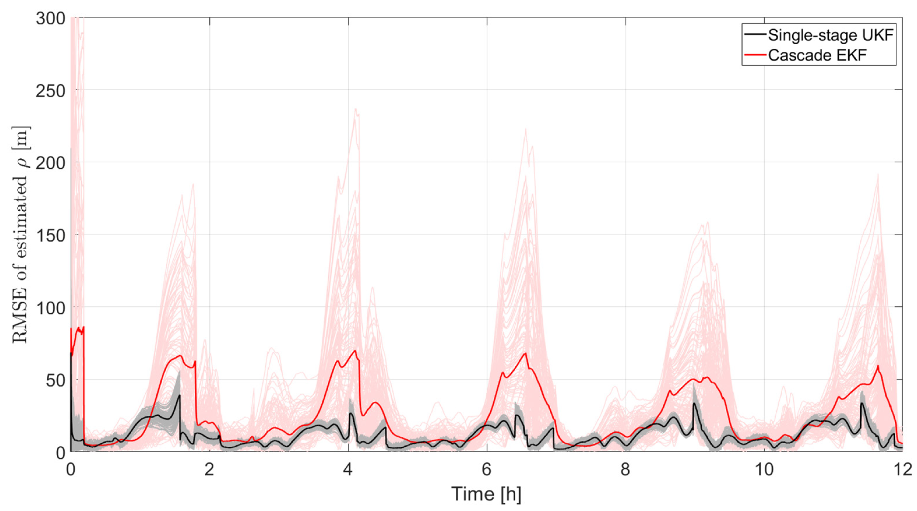
For a better practical understanding of the performance, this information is translated in relative position rather than relative orbital elements. The error norm obtained in the two Monte Carlo campaigns can be found in Figure 15 with the usual meaning of the colors. It is clear that the single-stage UKF outperforms the cascade EKF. Maximum errors can be as large as 300 m with this latter approach, while they reach 50 m in the newly proposed single-stage UKF. Also, for the relative distance estimate, it is confirmed that the cascade EKF suffers from a much larger variation among the different runs of the Monte Carlo campaign.
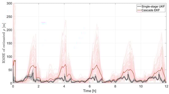
Figure 15.
Error norm of the estimated relative position with the single-stage UKF and the cascade EKF.
7. Conclusions
A navigation satellite system, providing navigation messages for lunar rovers and orbiters, is currently being investigated by major space agencies, with a particular focus on regions of greatest interest, i.e., the south pole of the Moon. In this research work, the possibility of further exploiting this service as a navigation system for the formation of satellites in lunar orbits is investigated.
A single-stage UKF is developed, estimating the relative position of the satellites of the formation taking directly the received pseudoranges into account. This is the main difference over already proposed cascade filters, which first estimate the inertial state of the satellites, and then apply a second filtering stage for improving the accuracy of the relative position.
The performance obtained with the presented filter, considering the difficulties that are specific to the lunar navigation satellite system (i.e., a very limited number of available measurements) is very promising and allows us to consider future formation flying missions that require navigation accuracy in the order of tens of meters. Integration with other navigation sensors, such as inter-satellite links and visual navigation, could further improve the presented performance. Indeed, more extensive studies are needed to consolidate and extend the results to a wider variety of cases, including the case of rovers moving on the lunar surface and specific mission phases such as the landing.
Author Contributions
Conceptualization, M.S.; methodology, M.S. and G.B.P.; software, M.S.; validation, M.S. and G.B.P.; formal analysis, M.S. and G.B.P.; investigation, M.S.; resources, M.S. and G.B.P.; data curation, M.S.; writing—original draft preparation, M.S.; writing—review and editing, M.S. and G.B.P.; visualization, M.S.; supervision, G.B.P. All authors have read and agreed to the published version of the manuscript.
Funding
This research received no external funding.
Data Availability Statement
Data are contained within the article.
Conflicts of Interest
The authors declare no conflict of interest.
References
- Smith, M.; Craig, D.; Herrmann, N.; Mahoney, E.; Krezel, J.; McIntyre, N.; Goodliff, K. The Artemis Program: An Overview of NASA’s Activities to Return Humans to the Moon. In Proceedings of the 2020 IEEE Aerospace Conference, Big Sky, MT, USA, 7–14 March 2020; pp. 1–10. [Google Scholar]
- Nie, T.; Gurfil, P.; Zhang, S. Lunar Satellite Formation Keeping Using Differential Solar Radiation Pressure. J. Guid. Control Dyn. 2020, 43, 754–766. [Google Scholar] [CrossRef]
- Sirbu, G.; Leonardi, M.; Stallo, C.; Di Lauro, C.; Carosi, M. Evaluation of different satellite navigation methods for the Moon in the future exploration age. Acta Astronaut. 2023, 208, 205–218. [Google Scholar] [CrossRef]
- Available online: https://www.esa.int/Applications/Telecommunications_Integrated_Applications/Moonlight (accessed on 24 May 2023).
- Iannone, C.; Carosi, M.; Eleuteri, M.; Stallo, C.; Di Lauro, C.; Musacchio, D. Four satellites to navigate the Moon’s South Pole: An Orbital Study. In Proceedings of the 34th International Technical Meeting of the Satellite Division of the Institute of Navigation (ION GNSS+ 2021), St. Louis, MO, USA, 20–24 September 2021. [Google Scholar]
- Giordano, P.; Grenier, A.; Zoccarato, P.; Bucci, L.; Cropp, A.; Swinden, R.; Otero, D.G.; El-Dali, W.; Carey, W.; Duvet, L.; et al. Moonlight navigation service—How to land on peaks of eternal light. In Proceedings of the 72nd International Astronautical Congress (IAC), Dubai, United Arab Emirates, 25–29 October 2021. [Google Scholar]
- Sabatini, M.; Gasbarri, P.; Palmerini, G.B. GNSS relative navigation for operations in cislunar space. In Proceedings of the Aerospace Europe Conference 2023—10th EUCASS—9th CEAS, Lausanne, Switzerland, 9–13 July 2023. [Google Scholar]
- Sirbu, G.; Leonardi, M.; Carosi, M.; Di Lauro, C.; Stallo, C. Performance evaluation of a lunar navigation system exploiting four satellites in ELFO orbits. In Proceedings of the 2022 IEEE 9th International Workshop on Metrology for AeroSpace (MetroAeroSpace), Pisa, Italy, 27–29 June 2022. [Google Scholar]
- Grenier, A. Positioning and Velocity Performance Levels for a Lunar Lander using a Dedicated Lunar Communication and Navigation System. Navig. J. Inst. Navig. 2022, 69, 2. [Google Scholar] [CrossRef]
- Vallado, D.A. Fundamental of Astrodynamics and Applications. In The Space Technology Library, 4th ed.; Microcosm Press: Cleveland, OH, USA, 1997. [Google Scholar]
- Rodriguez, F.; Martinelli, A.; Spazzacampagna, L.; Albanese, C.; Palmerini, G.B.; Sabatini, M. Analysis of PNT Algorithms and Related Performance for Lunar Navigation Service Users. In Proceedings of the 6th International Technical Meeting of the Satellite Division of The Institute of Navigation (ION GNSS+ 2023), Denver, CO, USA, 11–15 September 2023; pp. 3677–3697. [Google Scholar]
- Zarchan, P.; Musoff, H. Fundamental of kalman filtering. Prog. Astronaut. Aeronaut. 2000, 190, 225–259. [Google Scholar]
- Montenbruck, O.; Ramos-Bosch, P. Precision real-time navigation of LEO satellites using global positioning system measurements. GPS Solut. 2008, 12, 187–198. [Google Scholar] [CrossRef]
- Tang, J.; Wang, H.; Chen, Q.; Chen, Z.; Zheng, J.; Cheng, H.; Liu, L. A time-efficient implementation of Extended Kalman Filter for sequential orbit determination and a case study for onboard application. Adv. Space Res. 2018, 62, 343–358. [Google Scholar] [CrossRef]
- Lou, Y.; Dai, X.; Gong, X.; Li, C.; Qing, Y.; Liu, Y.; Peng, Y.; Gu, S. A review of real-time multi-GNSS precise orbit determination based on the filter method. Satell Navig. 2022, 3, 15. [Google Scholar] [CrossRef]
- Clohessy, W.H.; Wiltshire, R.S. Terminal guidance system for satellite rendezvous. J. Aero. Sci. 1960, 27, 653–678. [Google Scholar] [CrossRef]
- Sabatini, M.; Palmerini, G.B. Linearized Formation-Flying Dynamics in a Perturbed Orbital Environment. In Proceedings of the 2008 IEEE Aerospace Conference, Bigsky, MT, USA, 1–8 March 2008. [Google Scholar]
- Gaias, G.; Ardaens, J.S.; Montenbruck, O. Model of J2 perturbed satellite relative motion with time-varying differential drag. Celest. Mech. Dyn. Astr. 2015, 123, 411–433. [Google Scholar] [CrossRef]
- Simon, D. Optimal State Estimation: Kalman, H-inf and Nonlinear Approaches. In Wiley Interscience; John Wiley & Sons, Inc., Publication: Hoboken, NJ, USA, 2006. [Google Scholar]
- Reali, F.; Palmerini, G.B. Estimate Problems for Satellite Clusters. In Proceedings of the 2008 IEEE Aerospace Conference, Big Sky, MT, USA, 1–8 March 2008. [Google Scholar]
- Choi, E.-J.; Yoon, J.-C.; Lee, B.-S.; Park, S.-Y.; Choi, K.-H. Onboard orbit determination using GPS observations based on the unscented Kalman filter. Adv. Space Res. 2010, 46, 1440–1450. [Google Scholar] [CrossRef]


Disclaimer/Publisher’s Note: The statements, opinions and data contained in all publications are solely those of the individual author(s) and contributor(s) and not of MDPI and/or the editor(s). MDPI and/or the editor(s) disclaim responsibility for any injury to people or property resulting from any ideas, methods, instructions or products referred to in the content. |
© 2024 by the authors. Licensee MDPI, Basel, Switzerland. This article is an open access article distributed under the terms and conditions of the Creative Commons Attribution (CC BY) license (https://creativecommons.org/licenses/by/4.0/).