
Shape Morphing of 4D-Printed Polylactic Acid Structures under Thermal Stimuli: An Experimental and Finite Element Analysis


 ,
,  and
and 
Abstract
1. Introduction
2. Methodology
2.1. Materials and Methods
2.2. Design of Experiments
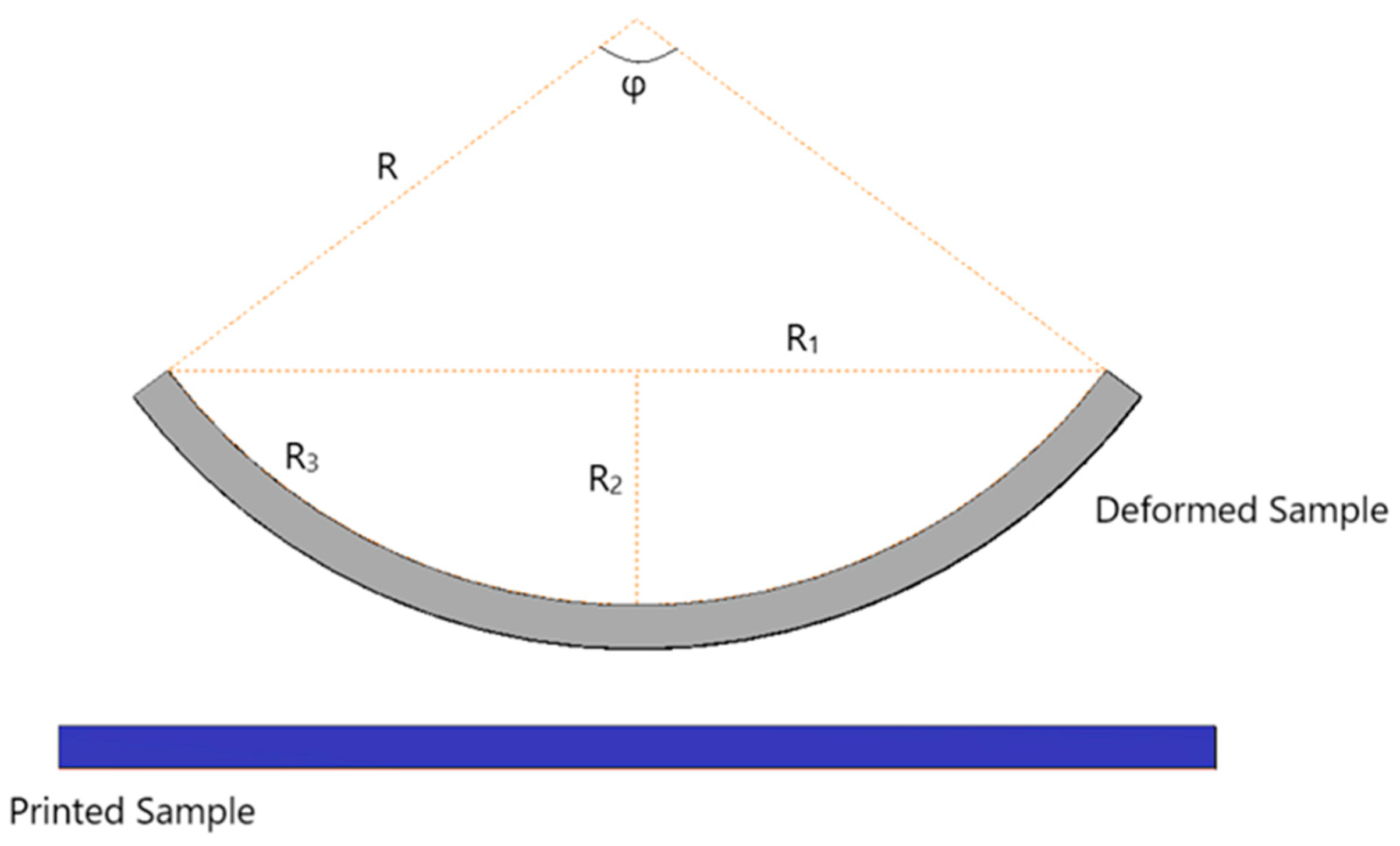
- R1—Chord of Deformed Structure: This parameter represents the straight line distance between the two ends of the curve, essentially measuring the overall length of the deformed structure;
- R2—Beam Deflection: R2 measures the extent of deviation or displacement of the beam from its original position. It is a critical indicator of the degree of deformation experienced by the structure;
- R3—Internal Arc: This parameter captures the curvature within the deformed shape, providing insights into the internal bending and shape changes of the structure.
2.3. Main Effect Analysis
2.4. Analysis of Variance (ANOVA)
- Total Degrees of Freedom: This is calculated using , where k represents the total number of experimental runs.
- Degrees of Freedom for Each Control Factor: Determined by , where i corresponds to each factor (A, B, C, D, E, F), and l is the total number of levels for each factor.
- Degrees of Freedom for Residual Error: Calculated using , where n is the number of control factors.
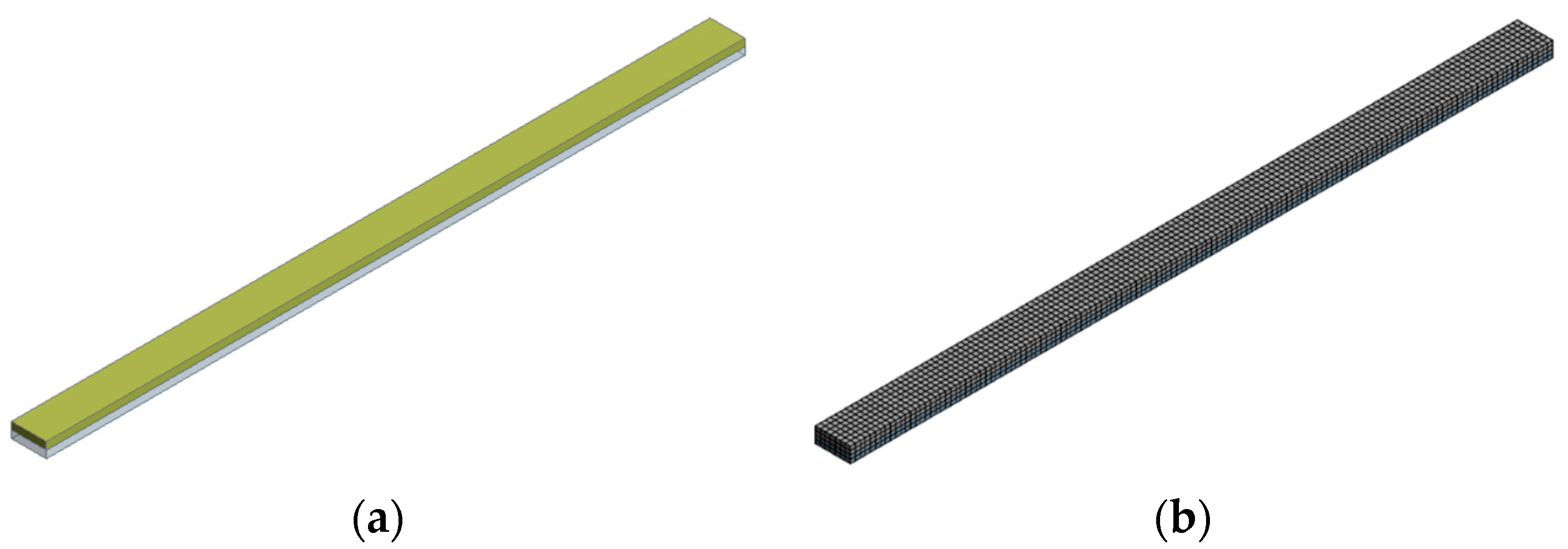
3. Finite Element Modelling
4. Results and Discussion
4.1. Experimental Results and Analysis
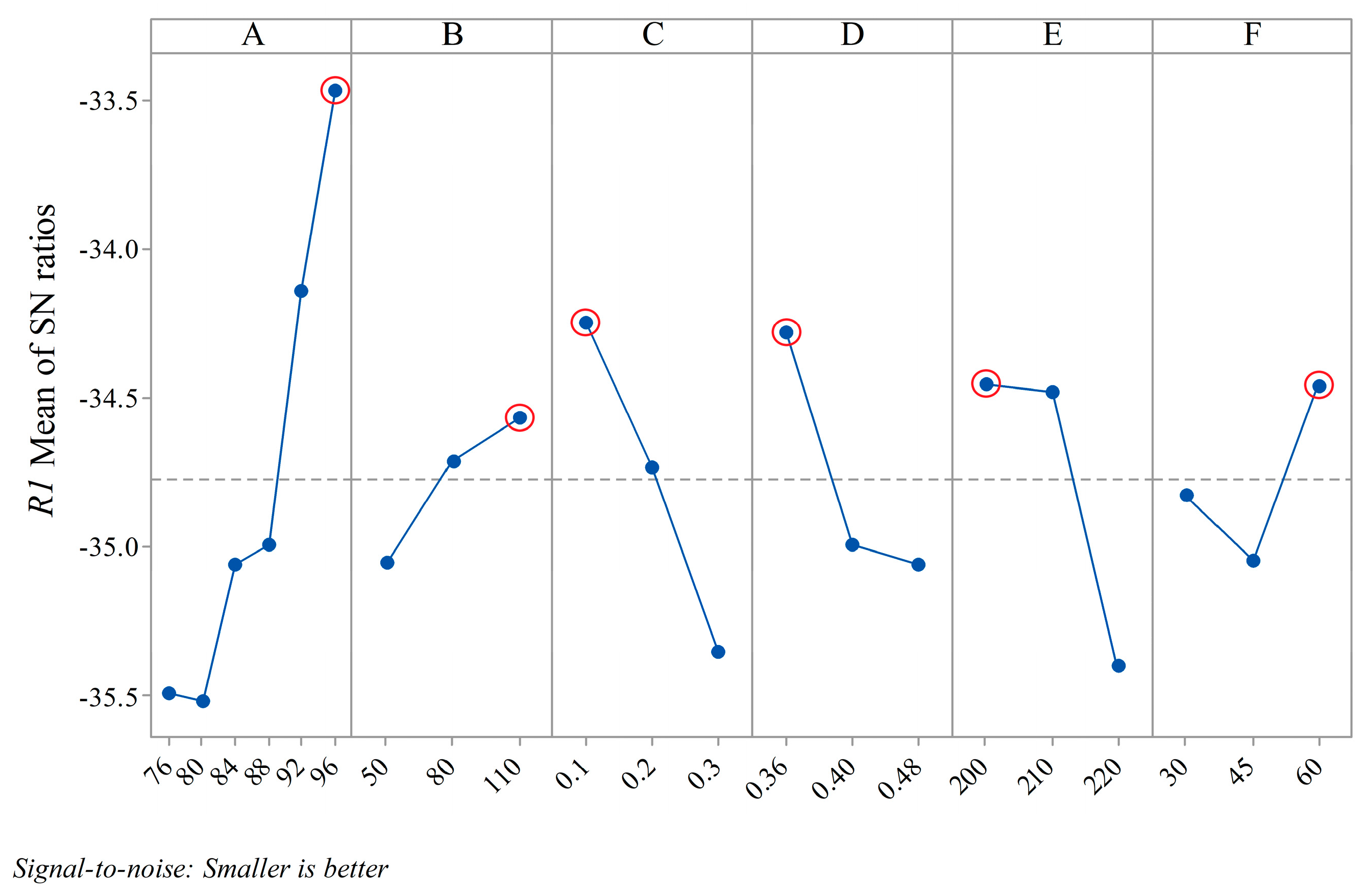
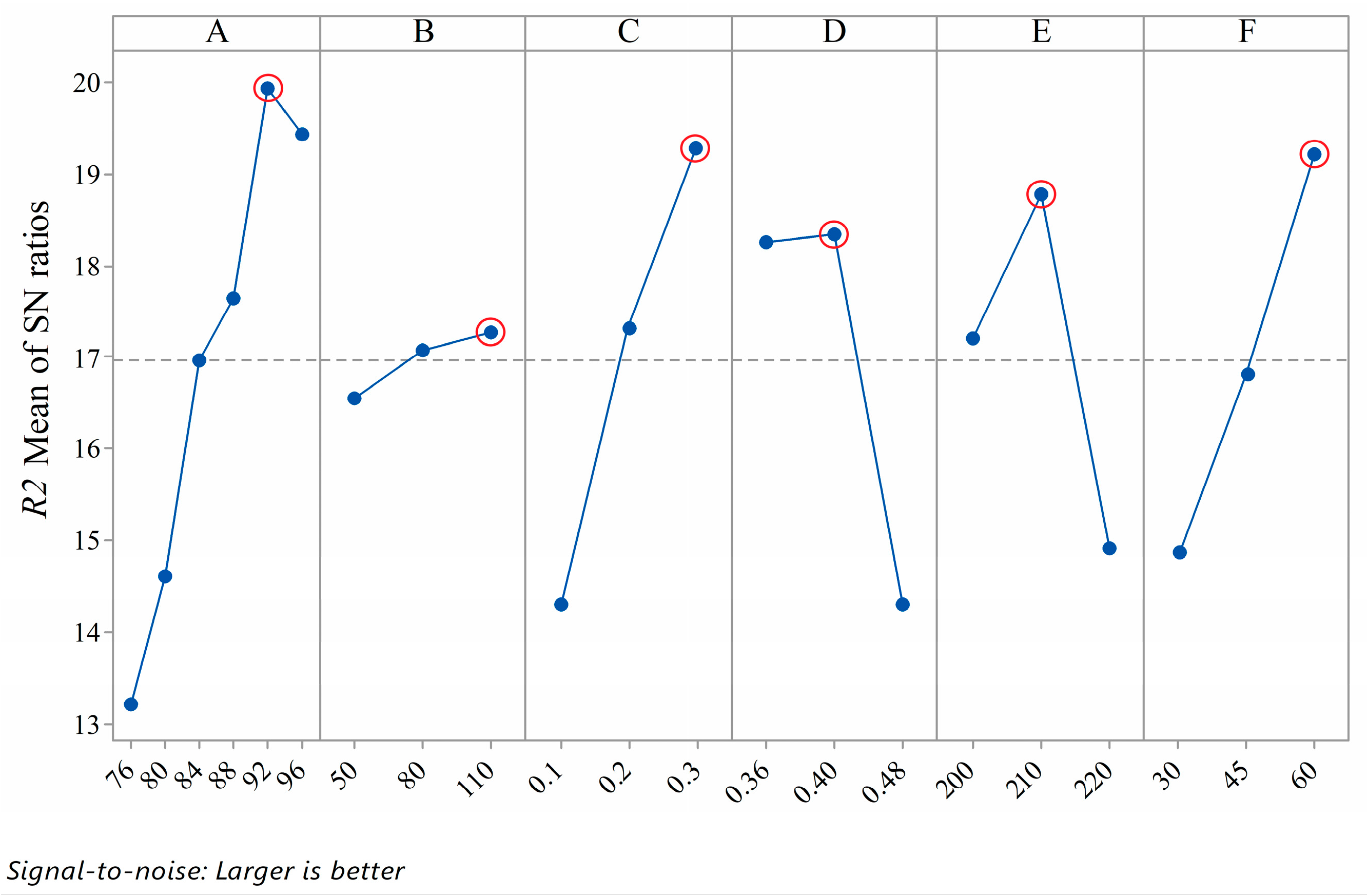
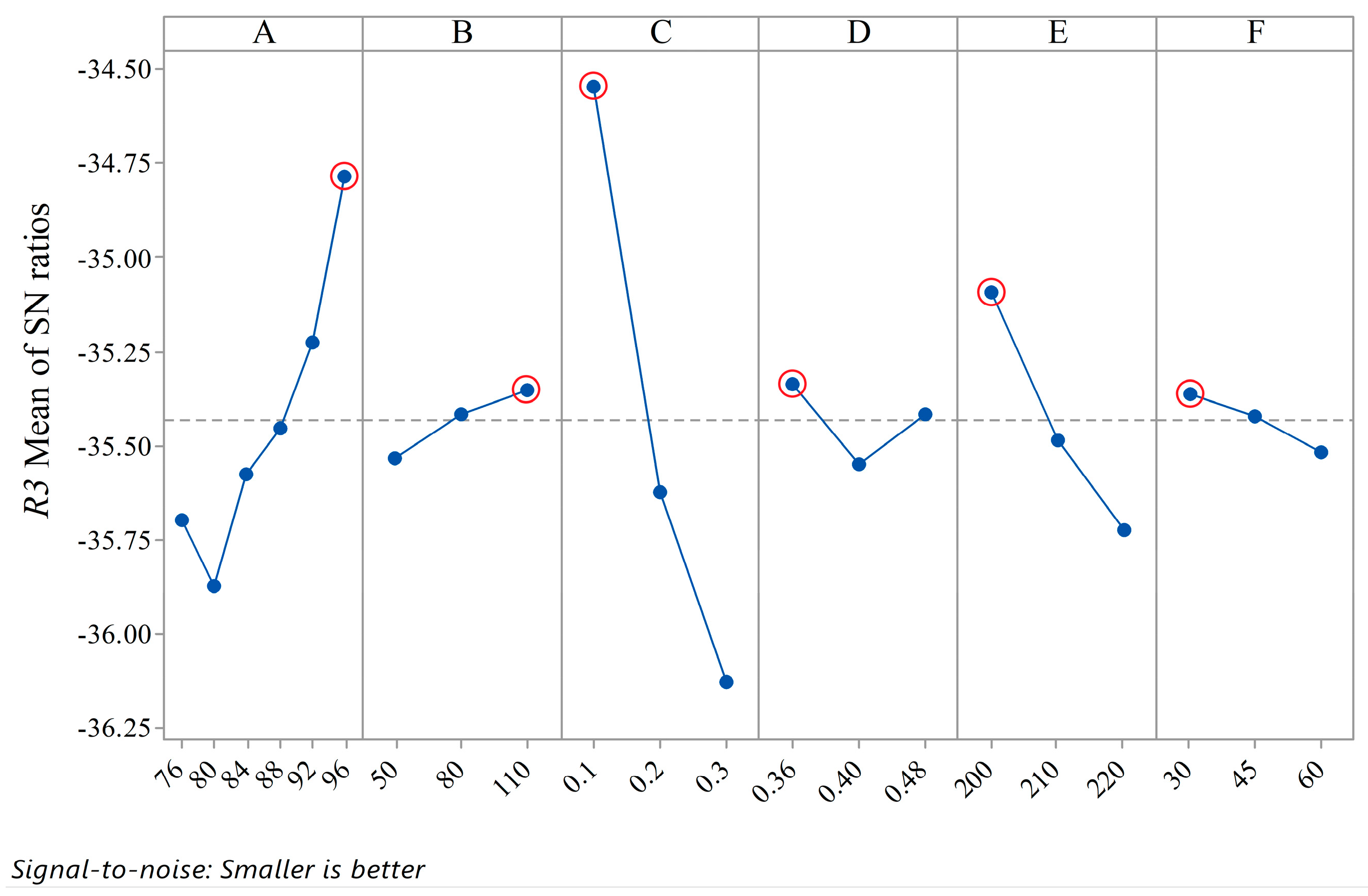
4.1.1. S/N Analysis
4.1.2. ANOVA
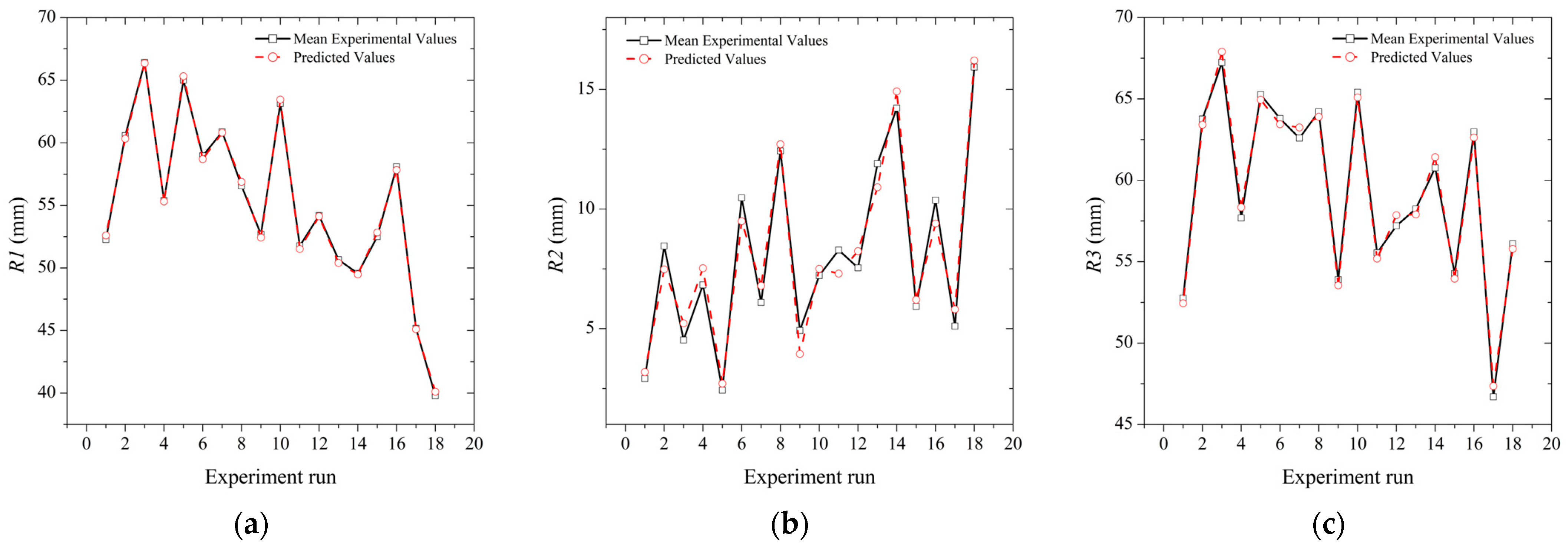
4.1.3. Regression Analysis
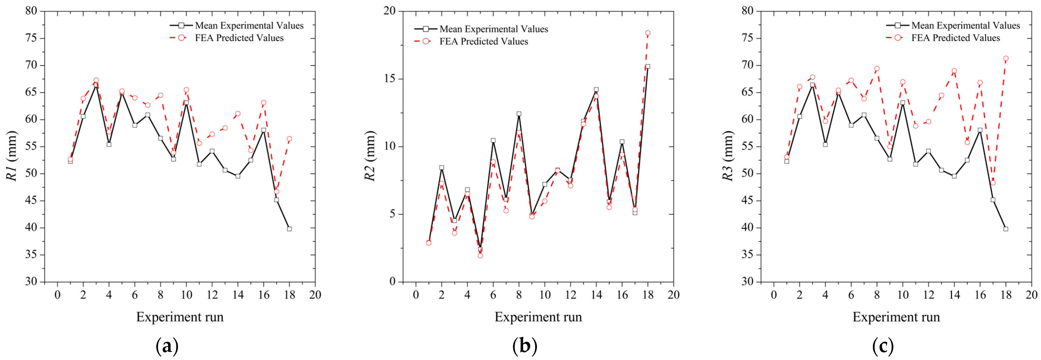
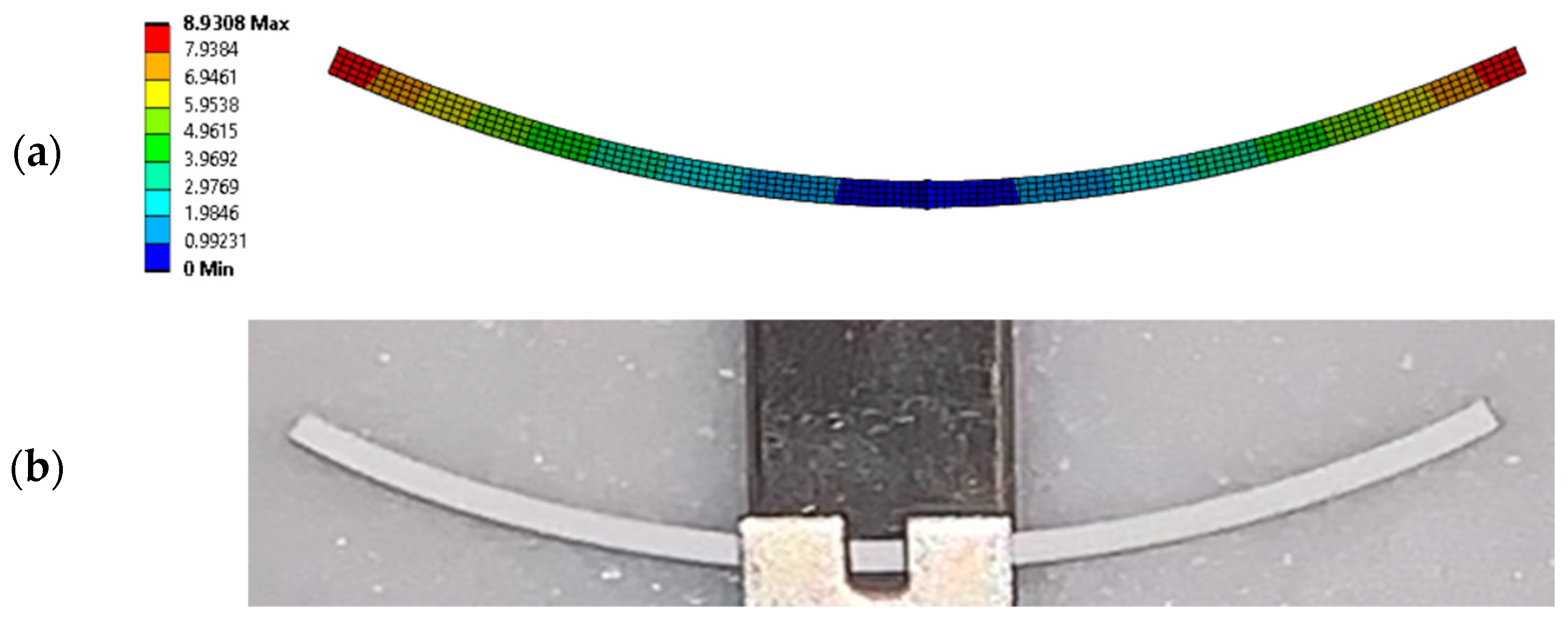
4.2. FEA Results
5. Conclusions
- Activation temperature and layer height emerged as significant factors influencing the shape-morphing behavior, as revealed by the S/N ratio analysis and ANOVA results;
- The precision in setting the printing speed, layer width, nozzle temperature, and bed temperature was found to be crucial in achieving the desired shape-morphing characteristics;
- Regression models developed for predicting the responses R1, R2, and R3 demonstrated strong correlations with observed data, highlighting the interplay between these printing parameters and the shape-morphing outcomes;
- The FEA modeling successfully predicted the performance of the structures, demonstrating its potential as an effective design tool in 4D printing;
- The ability of FEA modeling to closely predict the experimental outcomes suggests its utility in the design phase, allowing for the optimization of printing parameters before actual production.
Author Contributions
Funding
Data Availability Statement
Conflicts of Interest
References
- Momeni, F.; Liu, X.; Ni, J. A Review of 4D Printing. Mater. Des. 2017, 122, 42–79. [Google Scholar] [CrossRef]
- Chu, H.; Yang, W.; Sun, L.; Cai, S.; Yang, R.; Liang, W.; Yu, H.; Liu, L. 4D Printing: A Review on Recent Progresses. Micromachines 2020, 11, 796. [Google Scholar] [CrossRef] [PubMed]
- Kuang, X.; Roach, D.J.; Wu, J.; Hamel, C.M.; Ding, Z.; Wang, T.; Dunn, M.L.; Qi, H.J. Advances in 4D Printing: Materials and Applications. Adv. Funct. Mater. 2019, 29, 1805290. [Google Scholar] [CrossRef]
- Khalid, M.Y.; Arif, Z.U.; Noroozi, R.; Zolfagharian, A.; Bodaghi, M. 4D Printing of Shape Memory Polymer Composites: A Review on Fabrication Techniques, Applications, and Future Perspectives. J. Manuf. Process. 2022, 81, 759–797. [Google Scholar] [CrossRef]
- Yarali, E.; Baniasadi, M.; Zolfagharian, A.; Chavoshi, M.; Arefi, F.; Hossain, M.; Bastola, A.; Ansari, M.; Foyouzat, A.; Dabbagh, A.; et al. Magneto-/Electro-responsive Polymers toward Manufacturing, Characterization, and Biomedical/Soft Robotic Applications. Appl. Mater. Today 2022, 26, 101306. [Google Scholar] [CrossRef]
- Zafar, M.Q.; Zhao, H. 4D Printing: Future Insight in Additive Manufacturing. Met. Mater. Int. 2019, 26, 564–585. [Google Scholar] [CrossRef]
- Hua, M.; Wu, D.; Wu, S.; Ma, Y.; Alsaid, Y.; He, X. 4D Printable Tough and Thermoresponsive Hydrogels. ACS Appl. Mater. Interfaces 2021, 13, 12689–12697. [Google Scholar] [CrossRef]
- Zhang, Y.; Wang, Q.; Yi, S.; Lin, Z.; Wang, C.; Chen, Z.; Jiang, L. 4D Printing of Magnetoactive Soft Materials for On-Demand Magnetic Actuation Transformation. ACS Appl. Mater. Interfaces 2021, 13, 4174–4184. [Google Scholar] [CrossRef]
- Rastogi, P.; Kandasubramanian, B. Breakthrough in the Printing Tactics for Stimuli-Responsive Materials: 4D Printing. Chem. Eng. J. 2019, 366, 264–304. [Google Scholar] [CrossRef]
- Sonatkar, J.; Kandasubramanian, B.; Ismail, S.O. 4D Printing: Pragmatic Progression in Biofabrication. Eur. Polym. J. 2022, 169, 111128. [Google Scholar] [CrossRef]
- Akbar, I.; El Hadrouz, M.; El Mansori, M.; Lagoudas, D. Toward Enabling Manufacturing Paradigm of 4D Printing of Shape Memory Materials: Open Literature Review. Eur. Polym. J. 2022, 168, 111106. [Google Scholar] [CrossRef]
- Zhang, Z.; Demir, K.G.; Gu, G.X. Developments in 4D-Printing: A Review on Current Smart Materials, Technologies, and Applications. Int. J. Smart Nano Mater. 2019, 10, 205–224. [Google Scholar] [CrossRef]
- Kačergis, L.; Mitkus, R.; Sinapius, M. Influence of Fused Deposition Modeling Process Parameters on the Transformation of 4D Printed Morphing Structures. Smart Mater. Struct. 2019, 28, 105042. [Google Scholar] [CrossRef]
- Noroozi, R.; Bodaghi, M.; Jafari, H.; Zolfagharian, A.; Fotouhi, M. Shape-Adaptive Metastructures with Variable Bandgap Regions by 4D Printing. Polymers 2020, 12, 519. [Google Scholar] [CrossRef] [PubMed]
- Mahmood, A.; Akram, T.; Shenggui, C.; Chen, H. Revolutionizing Manufacturing: A Review of 4D Printing Materials, Stimuli, and Cutting-Edge Applications. Compos. B Eng. 2023, 266, 110952. [Google Scholar] [CrossRef]
- Khalid, M.Y.; Arif, Z.U.; Ahmed, W. 4D Printing: Technological and Manufacturing Renaissance. Macromol. Mater. Eng. 2022, 307, 2200003. [Google Scholar] [CrossRef]
- Jones, M.P.; Murali, G.G.; Laurin, F.; Robinson, P.; Bismarck, A. Functional Flexibility: The Potential of Morphing Composites. Compos. Sci. Technol. 2022, 230, 109792. [Google Scholar] [CrossRef]
- Sun, J.; Guan, Q.; Liu, Y.; Leng, J. Morphing Aircraft Based on Smart Materials and Structures: A State-of-the-Art Review. J. Intell. Mater. Syst. Struct. 2016, 27, 2289–2312. [Google Scholar] [CrossRef]
- Ashir, M.; Hindahl, J.; Nocke, A.; Cherif, C. Development of an Adaptive Morphing Wing Based on Fiber-Reinforced Plastics and Shape Memory Alloys. J. Ind. Text. 2020, 50, 114–129. [Google Scholar] [CrossRef]
- Ameta, K.L.; Solanki, V.S.; Singh, V.; Devi, A.P.; Chundawat, R.S.; Haque, S. Critical Appraisal and Systematic Review of 3D & 4D Printing in Sustainable and Environment-Friendly Smart Manufacturing Technologies. Sustain. Mater. Technol. 2022, 34, e00481. [Google Scholar] [CrossRef]
- Ntouanoglou, K.; Stavropoulos, P.; Mourtzis, D. 4D Printing Prospects for the Aerospace Industry: A Critical Review. Procedia Manuf. 2018, 18, 120–129. [Google Scholar] [CrossRef]
- Zhao, W.; Yue, C.; Liu, L.; Leng, J.; Liu, Y. Mechanical Behavior Analyses of 4D Printed Metamaterials Structures with Excellent Energy Absorption Ability. Compos. Struct. 2023, 304, 116360. [Google Scholar] [CrossRef]
- Ma, B.; Zhang, Y.; Li, J.; Chen, D.; Liang, R.; Fu, S.; Li, D. 4D Printing of Multi-Stimuli Responsive Rigid Smart Composite Materials with Self-Healing Ability. Chem. Eng. J. 2023, 466, 143420. [Google Scholar] [CrossRef]
- Brischetto, S.; Torre, R.; Ferro, C.G. Experimental Evaluation of Mechanical Properties and Machine Process in Fused Deposition Modelling Printed Polymeric Elements. Adv. Intell. Syst. Comput. 2020, 975, 377–389. [Google Scholar] [CrossRef]
- Zaman, U.K.U.; Boesch, E.; Siadat, A.; Rivette, M.; Baqai, A.A. Impact of Fused Deposition Modeling (FDM) Process Parameters on Strength of Built Parts Using Taguchi’s Design of Experiments. Int. J. Adv. Manuf. Technol. 2019, 101, 1215–1226. [Google Scholar] [CrossRef]
- Patil, P.; Singh, D.; Raykar, S.J.; Bhamu, J. Multi-Objective Optimization of Process Parameters of Fused Deposition Modeling (FDM) for Printing Polylactic Acid (PLA) Polymer Components. Mater. Today Proc. 2021, 45, 4880–4885. [Google Scholar] [CrossRef]
- Weber, R.; Kuhlow, M.; Spierings, A.B.; Wegener, K. 4D Printed Assembly of Sensors and Actuators in Complex Formed Metallic Lightweight Structures. J. Manuf. Process 2023, 90, 406–417. [Google Scholar] [CrossRef]
- Fallah, A.; Asif, S.; Gokcer, G.; Koc, B. 4D Printing of Continuous Fiber-Reinforced Electroactive Smart Composites by Coaxial Additive Manufacturing. Compos. Struct. 2023, 316, 117034. [Google Scholar] [CrossRef]
- Mahmood, A.; Akram, T.; Chen, H.; Chen, S. On the Evolution of Additive Manufacturing (3D/4D Printing) Technologies: Materials, Applications, and Challenges. Polymers 2022, 14, 4698. [Google Scholar] [CrossRef]
- Joshi, S.C.; Sheikh, A.A. 3D Printing in Aerospace and Its Long-Term Sustainability. Virtual Phys. Prototyp. 2015, 10, 175–185. [Google Scholar] [CrossRef]
- Jian, B.; Demoly, F.; Zhang, Y.; Qi, H.J.; André, J.C.; Gomes, S. Origami-Based Design for 4D Printing of 3D Support-Free Hollow Structures. Engineering 2022, 12, 70–82. [Google Scholar] [CrossRef]
- Tao, R.; Ji, L.; Li, Y.; Wan, Z.; Hu, W.; Wu, W.; Liao, B.; Ma, L.; Fang, D. 4D Printed Origami Metamaterials with Tunable Compression Twist Behavior and Stress-Strain Curves. Compos. B Eng. 2020, 201, 108344. [Google Scholar] [CrossRef]
- Liu, G.; Zhao, Y.; Wu, G.; Lu, J. Origami and 4D Printing of Elastomer-Derived Ceramic Structures. Sci. Adv. 2018, 4, 641–658. [Google Scholar] [CrossRef]
- Zhou, T.; Zhou, Y.; Hua, Z.; Yang, Y.; Zhou, C.; Ren, L.; Zhang, Z.; Zang, J. 4D Printing High Temperature Shape-Memory Poly(Ether–Ether–Ketone). Smart Mater. Struct. 2021, 30, 115006. [Google Scholar] [CrossRef]
- Zhang, J.; Yin, Z.; Ren, L.; Liu, Q.; Ren, L.; Yang, X.; Zhou, X. Advances in 4D Printed Shape Memory Polymers: From 3D Printing, Smart Excitation, and Response to Applications. Adv. Mater. Technol. 2022, 7, 2101568. [Google Scholar] [CrossRef]
- Zhang, B.; Li, H.; Cheng, J.; Ye, H.; Hosein Sakhaei, A.; Yuan, C.; Rao, P.; Zhang, Y.-F.; Chen, Z.; Wang, R.; et al. Mechanically Robust and UV-Curable Shape-Memory Polymers for Digital Light Processing Based 4D Printing. Adv. Mater. 2021, 33, 2101298. [Google Scholar] [CrossRef]
- Testoni, O.; Lumpe, T.; Huang, J.L.; Wagner, M.; Bodkhe, S.; Zhakypov, Z.; Spolenak, R.; Paik, J.; Ermanni, P.; Muñoz, L.; et al. A 4D Printed Active Compliant Hinge for Potential Space Applications Using Shape Memory Alloys and Polymers. Smart Mater. Struct. 2021, 30, 085004. [Google Scholar] [CrossRef]
- Costanza, G.; Tata, M.E. Shape Memory Alloys for Aerospace, Recent Developments, and New Applications: A Short Review. Materials 2020, 13, 1856. [Google Scholar] [CrossRef] [PubMed]
- Chen, S.; Li, J.; Shi, H.; Chen, X.; Liu, G.; Meng, S.; Lu, J. Lightweight and Geometrically Complex Ceramics Derived from 4D Printed Shape Memory Precursor with Reconfigurability and Programmability for Sensing and Actuation Applications. Chem. Eng. J. 2023, 455, 140655. [Google Scholar] [CrossRef]
- Liu, G.; Zhang, X.; Lu, X.; Zhao, Y.; Zhou, Z.; Xu, J.; Yin, J.; Tang, T.; Wang, P.; Yi, S.; et al. 4D Additive–Subtractive Manufacturing of Shape Memory Ceramics. Adv. Mater. 2023, 35, 2302108. [Google Scholar] [CrossRef] [PubMed]
- Patadiya, J.; Gawande, A.; Joshi, G.; Kandasubramanian, B. Additive Manufacturing of Shape Memory Polymer Composites for Futuristic Technology. Ind. Eng. Chem. Res. 2021, 60, 15885–15912. [Google Scholar] [CrossRef]
- Pyo, Y.; Kang, M.; Jang, J.Y.; Park, Y.; Son, Y.H.; Choi, M.C.; Ha, J.W.; Chang, Y.W.; Lee, C.S. Design of a Shape Memory Composite(SMC) Using 4D Printing Technology. Sens. Actuators A Phys. 2018, 283, 187–195. [Google Scholar] [CrossRef]
- Pivar, M.; Gregor-Svetec, D.; Muck, D. Effect of Printing Process Parameters on the Shape Transformation Capability of 3D Printed Structures. Polymers 2022, 14, 117. [Google Scholar] [CrossRef] [PubMed]
- Solomon, I.J.; Sevvel, P.; Gunasekaran, J. A Review on the Various Processing Parameters in FDM. Mater. Today Proc. 2021, 37, 509–514. [Google Scholar] [CrossRef]
- Nam, S.; Pei, E. The Influence of Shape Changing Behaviors from 4D Printing through Material Extrusion Print Patterns and Infill Densities. Materials 2020, 13, 3754. [Google Scholar] [CrossRef] [PubMed]
- Methods and Formulas for Analyze Taguchi Design—Minitab. Available online: https://support.minitab.com/en-us/minitab/21/help-and-how-to/statistical-modeling/doe/how-to/taguchi/analyze-taguchi-design/methods-and-formulas/methods-and-formulas/ (accessed on 16 June 2023).
- Montgomery, D.C. Design and Analysis of Experiments; Wiley: Hoboken, NJ, USA, 2019; 688p, ISBN 978-1-119-49244-3. [Google Scholar]
- Bademlioglu, A.H.; Canbolat, A.S.; Yamankaradeniz, N.; Kaynakli, O. Investigation of Parameters Affecting Organic Rankine Cycle Efficiency by Using Taguchi and ANOVA Methods. Appl. Therm. Eng. 2018, 145, 221–228. [Google Scholar] [CrossRef]
- Cheah, D.S.; Alshebly, Y.S.; Mohamed Ali, M.S.; Nafea, M. Development of 4D-Printed Shape Memory Polymer Large-Stroke XY Micropositioning Stages. J. Micromech. Microeng. 2022, 32, 065006. [Google Scholar] [CrossRef]
- Alshebly, Y.S.; Nafea, M. Effects of Printing Parameters on 4D-Printed PLA Actuators. Smart Mater. Struct. 2023, 32, 064008. [Google Scholar] [CrossRef]


| Code | Control Parameters | Unit | Level 1 | Level 2 | Level 3 | Level 4 | Level 5 | Level 6 |
|---|---|---|---|---|---|---|---|---|
| A | Activation Temperature | °C | 76 | 80 | 84 | 88 | 92 | 96 |
| B | Printing Speed | mm/s | 50 | 80 | 110 | - | - | - |
| C | Layer Height | mm | 0.1 | 0.2 | 0.3 | - | - | - |
| D | Layer Width | mm | 0.36 | 0.4 | 0.48 | - | - | - |
| E | Nozzle Temperature | °C | 200 | 210 | 220 | - | - | - |
| F | Bed Temperature | °C | 30 | 45 | 60 | - | - | - |
| Experiment Run | Activation Temperature (°C) | Printing Speed (mm/s) | Layer Height (mm) | Layer Width (mm) | Nozzle Temperature (°C) | Bed Temperature (°C) |
|---|---|---|---|---|---|---|
| 1 | 76 | 50 | 0.1 | 0.36 | 200 | 30 |
| 2 | 76 | 80 | 0.2 | 0.4 | 210 | 45 |
| 3 | 76 | 110 | 0.3 | 0.48 | 220 | 60 |
| 4 | 80 | 50 | 0.1 | 0.4 | 210 | 60 |
| 5 | 80 | 80 | 0.2 | 0.48 | 220 | 30 |
| 6 | 80 | 110 | 0.3 | 0.36 | 200 | 45 |
| 7 | 84 | 50 | 0.2 | 0.36 | 220 | 45 |
| 8 | 84 | 80 | 0.3 | 0.4 | 200 | 60 |
| 9 | 84 | 110 | 0.1 | 0.48 | 210 | 30 |
| 10 | 88 | 50 | 0.3 | 0.48 | 210 | 45 |
| 11 | 88 | 80 | 0.1 | 0.36 | 220 | 60 |
| 12 | 88 | 110 | 0.2 | 0.4 | 200 | 30 |
| 13 | 92 | 50 | 0.2 | 0.48 | 200 | 60 |
| 14 | 92 | 80 | 0.3 | 0.36 | 210 | 30 |
| 15 | 92 | 110 | 0.1 | 0.4 | 220 | 45 |
| 16 | 96 | 50 | 0.3 | 0.4 | 220 | 30 |
| 17 | 96 | 80 | 0.1 | 0.48 | 200 | 45 |
| 18 | 96 | 110 | 0.2 | 0.36 | 210 | 60 |
| Code | DoF | Sum of Squares | Mean Squares | F | p | Contribution (%) |
|---|---|---|---|---|---|---|
| A | 5 | 9.938 | 1.988 | 42.640 | 0.023 | 46.8 |
| B | 2 | 0.752 | 0.376 | 8.060 | 0.110 | 3.5 |
| C | 2 | 3.698 | 1.849 | 39.670 | 0.025 | 17.4 |
| D | 2 | 2.238 | 1.119 | 24.010 | 0.040 | 10.5 |
| E | 2 | 3.462 | 1.731 | 37.130 | 0.026 | 16.3 |
| F | 2 | 1.050 | 0.525 | 11.270 | 0.082 | 4.9 |
| Residual error | 2 | 0.093 | 0.047 | - | - | 0.4 |
| Total | 17 | 21.231 | - | - | - | 100.0 |
| Code | DoF | Sum of Squares | Mean Squares | F | p | Contribution (%) |
|---|---|---|---|---|---|---|
| A | 5 | 104.909 | 20.982 | 1.350 | 0.476 | 27.7 |
| B | 2 | 1.677 | 0.839 | 0.050 | 0.949 | 0.4 |
| C | 2 | 75.979 | 37.990 | 2.450 | 0.290 | 20.1 |
| D | 2 | 63.356 | 31.678 | 2.040 | 0.329 | 16.7 |
| E | 2 | 44.837 | 22.419 | 1.450 | 0.409 | 11.8 |
| F | 2 | 56.876 | 28.438 | 1.840 | 0.353 | 15.0 |
| Residual error | 2 | 30.995 | 15.497 | - | - | 8.2 |
| Total | 17 | 378.628 | - | - | - | 100.0 |
| Code | DoF | Sum of Squares | Mean Squares | F | p | Contribution (%) |
|---|---|---|---|---|---|---|
| A | 5 | 2.240 | 0.448 | 7.600 | 0.120 | 19.0 |
| B | 2 | 0.104 | 0.052 | 0.880 | 0.532 | 0.9 |
| C | 2 | 7.855 | 3.927 | 66.650 | 0.015 | 66.8 |
| D | 2 | 0.138 | 0.069 | 1.170 | 0.461 | 1.2 |
| E | 2 | 1.234 | 0.617 | 10.470 | 0.087 | 10.5 |
| F | 2 | 0.074 | 0.037 | 0.620 | 0.616 | 0.6 |
| Residual error | 2 | 0.118 | 0.059 | 1.0 | ||
| Total | 17 | 11.762 | 100 |
| Experiment Run | at (°C−1) | ab (°C−1) |
|---|---|---|
| 1 | −4.98 × 10⁻³ | −4.88 × 10⁻³ |
| 2 | −1.70 × 10⁻³ | −1.46 × 10⁻³ |
| 3 | −7.45 × 10⁻⁴ | −6.26 × 10⁻⁴ |
| 4 | −3.22 × 10⁻³ | −3.02 × 10⁻³ |
| 5 | −1.25 × 10⁻³ | −1.19 × 10⁻³ |
| 6 | −1.53 × 10⁻³ | −1.26 × 10⁻³ |
| 7 | −1.78 × 10⁻³ | −1.63 × 10⁻³ |
| 8 | −1.29 × 10⁻³ | −9.78 × 10⁻⁴ |
| 9 | −3.97 × 10⁻³ | −3.83 × 10⁻³ |
| 10 | −9.98 × 10⁻⁴ | −8.40 × 10⁻⁴ |
| 11 | −3.28 × 10⁻³ | −3.06 × 10⁻³ |
| 12 | −2.90 × 10⁻³ | −2.71 × 10⁻³ |
| 13 | −2.44 × 10⁻³ | −2.15 × 10⁻³ |
| 14 | −1.85 × 10⁻³ | −1.51 × 10⁻³ |
| 15 | −3.38 × 10⁻³ | −3.24 × 10⁻³ |
| 16 | −1.35 × 10⁻³ | −1.13 × 10⁻³ |
| 17 | −4.75 × 10⁻³ | −4.62 × 10⁻³ |
| 18 | −2.67 × 10⁻³ | −2.24 × 10⁻³ |
Disclaimer/Publisher’s Note: The statements, opinions and data contained in all publications are solely those of the individual author(s) and contributor(s) and not of MDPI and/or the editor(s). MDPI and/or the editor(s) disclaim responsibility for any injury to people or property resulting from any ideas, methods, instructions or products referred to in the content. |
© 2024 by the authors. Licensee MDPI, Basel, Switzerland. This article is an open access article distributed under the terms and conditions of the Creative Commons Attribution (CC BY) license (https://creativecommons.org/licenses/by/4.0/).
Share and Cite
Kostopoulos, G.; Stamoulis, K.; Lappas, V.; Georgantzinos, S.K. Shape Morphing of 4D-Printed Polylactic Acid Structures under Thermal Stimuli: An Experimental and Finite Element Analysis. Aerospace 2024, 11, 134. https://doi.org/10.3390/aerospace11020134
Kostopoulos G, Stamoulis K, Lappas V, Georgantzinos SK. Shape Morphing of 4D-Printed Polylactic Acid Structures under Thermal Stimuli: An Experimental and Finite Element Analysis. Aerospace. 2024; 11(2):134. https://doi.org/10.3390/aerospace11020134
Chicago/Turabian StyleKostopoulos, Grigorios, Konstantinos Stamoulis, Vaios Lappas, and Stelios K. Georgantzinos. 2024. "Shape Morphing of 4D-Printed Polylactic Acid Structures under Thermal Stimuli: An Experimental and Finite Element Analysis" Aerospace 11, no. 2: 134. https://doi.org/10.3390/aerospace11020134
APA StyleKostopoulos, G., Stamoulis, K., Lappas, V., & Georgantzinos, S. K. (2024). Shape Morphing of 4D-Printed Polylactic Acid Structures under Thermal Stimuli: An Experimental and Finite Element Analysis. Aerospace, 11(2), 134. https://doi.org/10.3390/aerospace11020134