Transonic Buffet Suppression by Airfoil Optimization

Abstract

The main buffet suppression techniques of aircrafts include active and passive flow control, aiming to reduce the impact of the fluctuating loads on the airfoil. These techniques are remedies after the airfoil design. The buffet suppression is not always considered in the aerodynamic optimization in the state of airfoil design because it is difficult to extract an appropriate key objective variable to indicate the flow stability. In this paper, the damping rate of disturbance, which is computed by the global stability analysis, can be used to indicate flow stability. Based on the global stability analysis, a transonic buffet suppression methodology by airfoil optimization is proposed. The objective is to improve the aerodynamic performance as well as the flow stability in the desired flight state. The RAE2822 airfoil is chosen as the initial airfoil. A benchmark of the unsteady aerodynamic configuration optimization design considering buffet suppression is developed. First, the numerical methods are verified and the damping rate of disturbance is chosen as a constraint in the aerodynamic optimization to extend the buffet onset. Then, the surrogate models constructed by the radial basis function interpolation are used to replace the computational fluid dynamics (CFD) solver. The teaching- and learning-based optimization (TLBO) is used. Finally, the aerodynamic and the flow stability characteristics of the airfoil before and after optimization are compared and analyzed. The proposed optimization framework can not only improve the aerodynamic characteristics in the cruise state but can also suppress the transonic buffet on higher angles of attack.

1. Introduction

The flow around the wing in transonic flow can easily become unstable at certain combinations of Mach number and angle of attack because of the interaction between the shock wave and the boundary layer, which would cause the transonic buffet problem. Transonic buffet, also called the shock buffet, is a typical self-excited oscillation [1]. The large amplitude oscillation of the shock load appears when the transonic buffet occurs. This not only diminishes the fatigue life of the aircraft and the ride quality, but also affects the function of the onboard instrumentation equipment and the use of flight control systems. Consequently, it can cause a flight safety hazard. Therefore, transonic buffet and its suppression have attracted considerable research interests in the aviation industry.

The recent main technique of buffet suppression is active or passive flow control, both of which aim to postpone buffet onset and mitigate shock oscillations without lowering aerodynamic performance. The basic idea of the transonic buffet control is to change the environment of the boundary layer and trailing edge. Passive control methods such as a streamwise slot [2], shock control bump [3,4,5], vortex generators [6], upper trailing-edge flap [7] and buffet breather [8,9] change the boundary layer environment. These passive controllers apply a small change to the original configuration, however, these techniques may cause poor aerodynamic performance in off-design flow conditions and can hardly eliminate the transonic buffet in designed flow conditions. Active control devices such as the trailing edge deflector [10,11], fluidic vortex generator [12] and trailing-edge flap [13] change the trailing edge environment. These techniques have a better effect on buffet suppression, while the control laws are complex and difficult to find. Moreover, the buffet control technique is actually the last choice after the finalization of the design. How to suppress the buffet in the stage of aircraft design remains to be studied. The aircraft designers would prefer to constrain the transonic buffet-onset in the early stages of the airfoil/wing design.

For this purpose, a transonic buffet suppression methodology by airfoil optimization is necessary in the stage of airfoil design. The existing research in the shape optimization of aircraft mainly focuses on the aerodynamic performance in the cruising state [14,15]. Recently, the buffet has been considered in the CFD-based aerodynamic shape optimization. Martins [16] constrained the buffet onset in an aerodynamic shape optimization by developing a separation-based constraint formulation, but it is a steady aerodynamic shape optimization essentially and the separation metric cannot indicate the flow stability accurately. The unsteady airfoil optimization considering buffet suppression is inaugurated by Thomas and Dowell [17,18], who optimized the geometric design by using the discrete adjoint method to minimize unsteady aerodynamic response near the buffet onset boundary. The unsteady aerodynamic response is computed by the forced vibration of plunge and pitch motion. The harmonic balance method is used to improve the efficiency. This work shows the way to increase the buffet onset angle of attack by unsteady airfoil optimization and as a result, the buffet onset is increased effectively. The lift-drag characteristics are not considered in the airfoil optimization and there is no specific analysis of optimized results. Xu [19] and Chen [20] consider the buffet effect in the optimal design of supercritical airfoil. The buffet amplitude is chosen as the objective or a constraint to indicate the flow stability, but it is only effective when buffet occurs in the design state. It is computationally costly to get the buffet amplitude. In the [19], the buffet are suppressed but not eliminated in the designed flow states.

It is difficult to extract a key design target to indicate the flow stability when an unsteady flow problem, such as transonic buffet, is considered in the shape design optimization. Furthermore, the unsteady RANS equations should be solved for the buffet simulation to extract the flow characteristics in the shape optimization, which is computationally costly. Recently, Chen [21] enhanced the aeroelastic stability of NACA0012 airfoil in the aerodynamic shape optimization. The pitch aerodynamic damping derivative can indicate the stability of the fluid-structure interaction system efficiently. It is adopted as the goal of shape optimization to avoid the occurrence of transonic buzz. Therefore, we intend to find a parameter to be the constraint of the shape optimization that can be efficiently obtained and also indicate the flow stability without human experience. The aerodynamic performance is improved in the design state and the buffet onset is delayed after airfoil optimization.

The transonic buffet involves several complex phenomena such as separated flow, shock-boundary layer interaction and turbulence. Its main research techniques are wind tunnel experiments and numerical simulations. The CFD technique has been fully developed since the 1990s, however, the unsteady Reynolds-averaged Navier–Stokes (URANS) equations based on the turbulence model have been developed and widely used in the simulation of the transonic buffet flow [22] more recently. In order to study the effects of the broadband turbulent spectrum, detached-eddy simulation (DES) [23], large-eddy simulation (LES) [24] and direct numerical simulation (DNS) [25] were developed to compute the transonic flow. Recently, DES was used by Li [26] for the buffet numerical simulation. Results show that the buffet root-mean-square value of the fluctuating pressure computed by DES is closer to the experimental results compared with URANS. Lipanov [27] got the accurate high-speed buffet onset by DNS. The time-domain simulation method can predict the buffet onset and buffet amplitude. However, it requires large computational costs and cannot directly provide the flow field stability characteristics such as aerodynamic damping and fluid modes. As a result, the reduced order models (ROM) such as auto regressive with eXogenous input (ARX) model [28], proper orthogonal decomposition (POD) method [29,30] and dynamic mode decomposition (DMD) method [31] were developed to extract the flow field characteristics in the time-domain simulation of the transonic buffet. However, this technique still needs many computations of training samples and a proper sample range.

The global stability analysis method based on the global instability theory can obtain the flow field characteristics directly and efficiently. This technique can be used to predict the instability onset and study the evolution law of the flow field characteristics. The stability is called global in order to describe the analysis of flows indicated by two- (BiGlobal) or three-dimensional (TriGlobal) inhomogeneous functions, the basic state of which is non-parallel from the ones described by one inhomogeneous spatial direction (local theory). Much progress has been made since the first publication of the global stability analysis by Pierrehumbert and Widnall [32]. Consequently, this technique has been applied to different practical problems, such as flow around a circular cylinder [33], stall at a high angle of attack [34,35] and transonic buffet [36,37,38] effectively. Theofilis [39,40] summarized the research progress of global stability analysis and reviewed the development directions in the future. The TriGlobal stability analysis has been used by researchers recently and various laws of flow field characteristics have been found [41,42]. For the engineering problem of transonic buffet, the stability analysis technique is mainly used to compute the buffet onset and the flow field characteristics such as the buffet frequency and fluid modes. However, the global stability analysis has not been used for the buffet suppression so far. The damping rate of disturbance computed by the global stability analysis can indicate the stability characteristics of transonic flow. Therefore, it is chosen to be a constraint of the shape optimization.

A transonic buffet suppression technique by airfoil optimization based on global stability analysis has been developed in the present work. The objective is to improve the aerodynamic performance and the flow stability of the airfoil in the design state. The drag coefficient is chosen as the objective parameter in the airfoil optimization to improve the aerodynamic performance, and the damping rate of disturbance is chosen as a constraint to delay the buffet onset. This allows the aircraft to perform a maneuver overload in cruise flight without buffet 1.3 times, which is required in aerospace engineering. The framework of buffet suppression methodology by airfoil optimization is introduced in Section 2. The optimized airfoils are compared with the initial airfoil and other optimized airfoils in reference. The similarities and differences in geometries, aerodynamic performance and buffet boundary are discussed and analyzed.

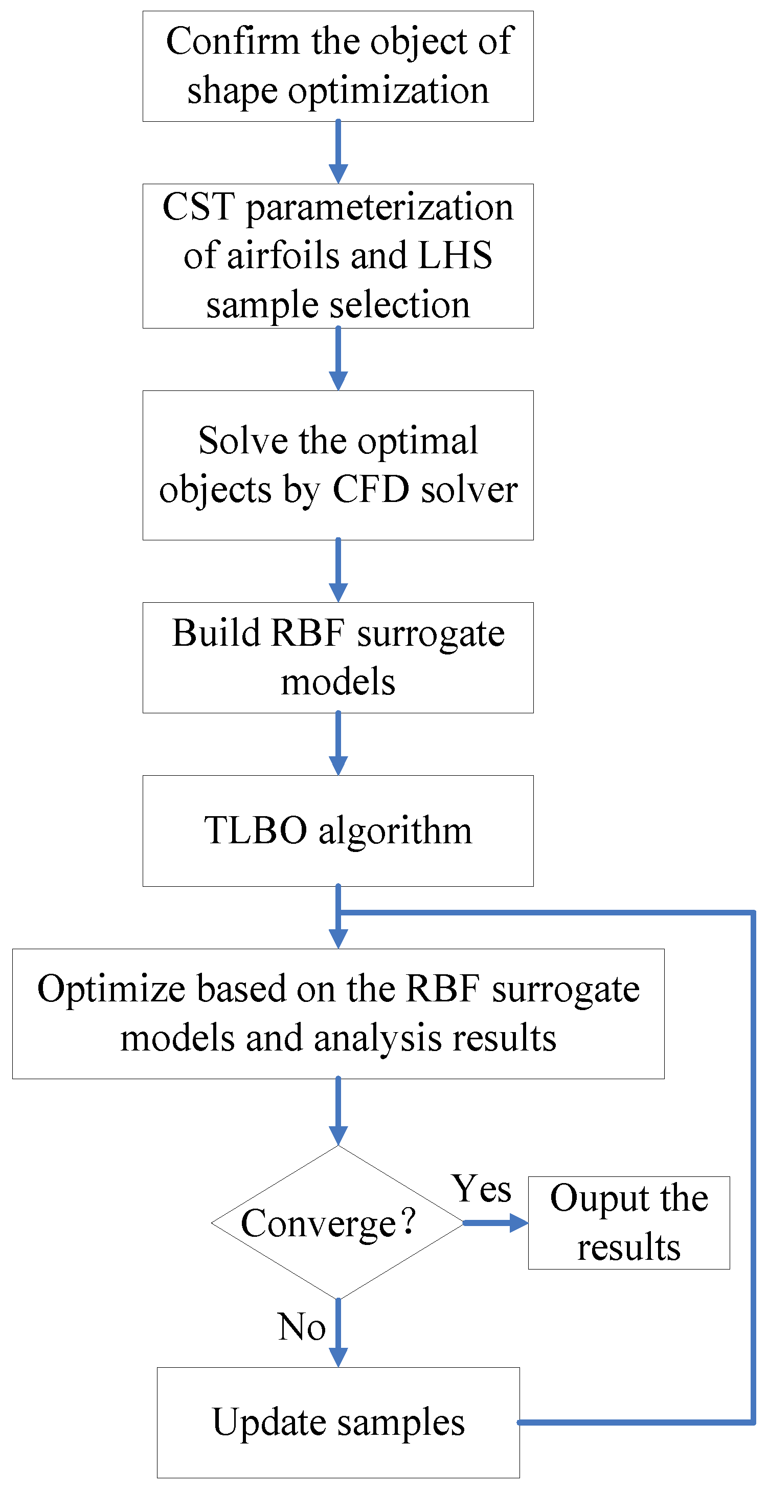
2. Optimization Framework

Figure 1 shows the optimization framework of this paper. The objective of this buffet suppression methodology is to optimize the airfoil in terms of aerodynamic performance and flow stability.

The drag coefficient is chosen as the objective parameter of the shape optimization. The damping rate of disturbance computed by the global stability analysis is chosen as a constraint. Then, the parameters obtained by the class-shape function transformation (CST) parameterization of the airfoil are chosen as the design variables. To improve the optimization efficiency, the surrogate models based on the radial basis function (RBF) interpolation are used to replace the CFD solver. Latin hypercube sampling (LHS) is used to select samples. Finally, the teaching- and learning-based optimization (TLBO) is used to obtain the optimal solution based on the RBF surrogate model.

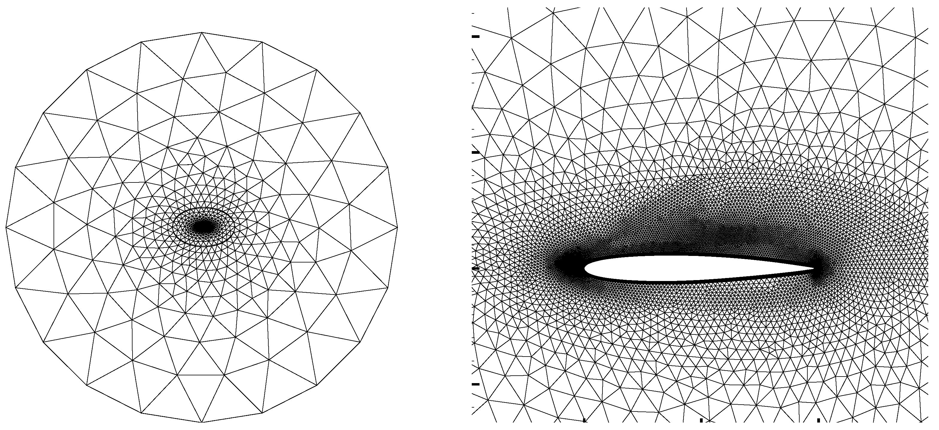
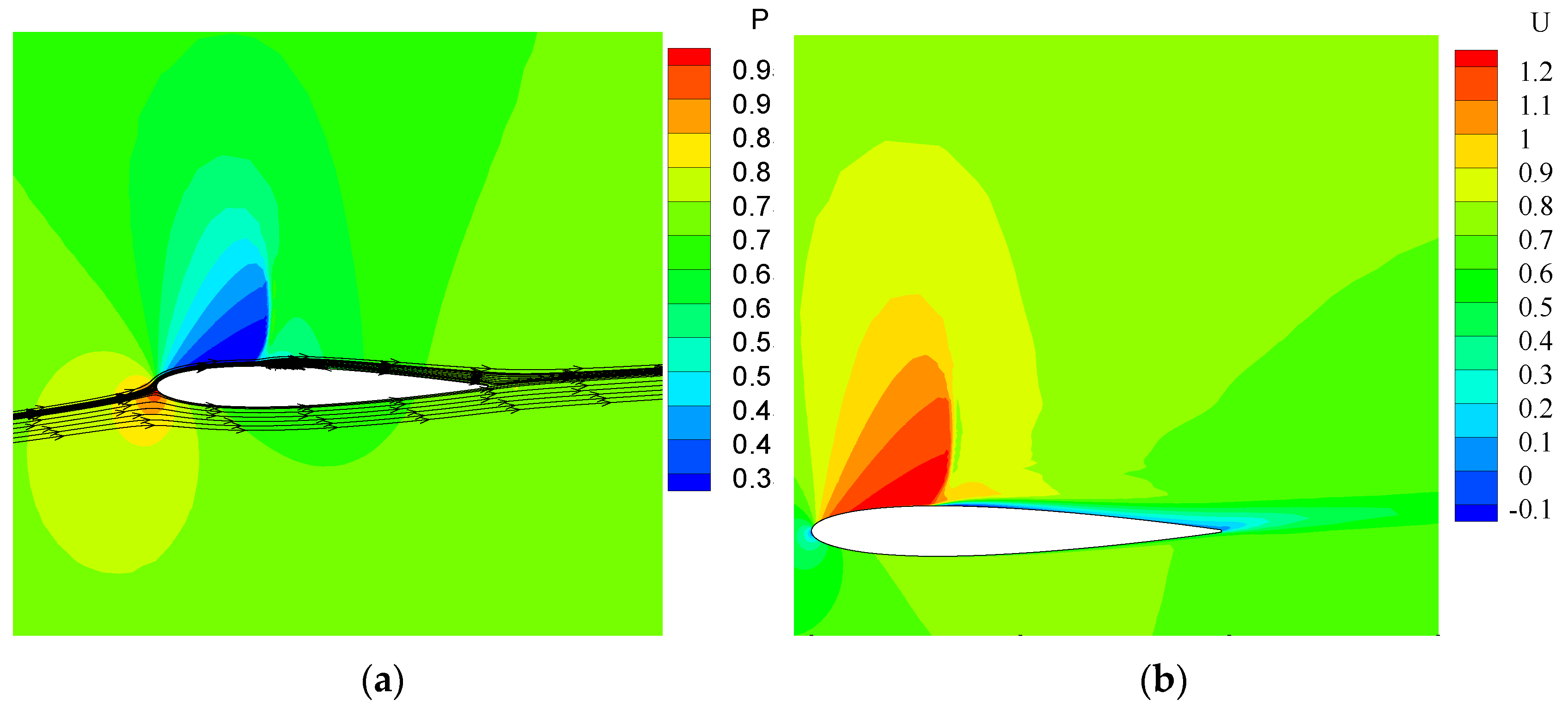
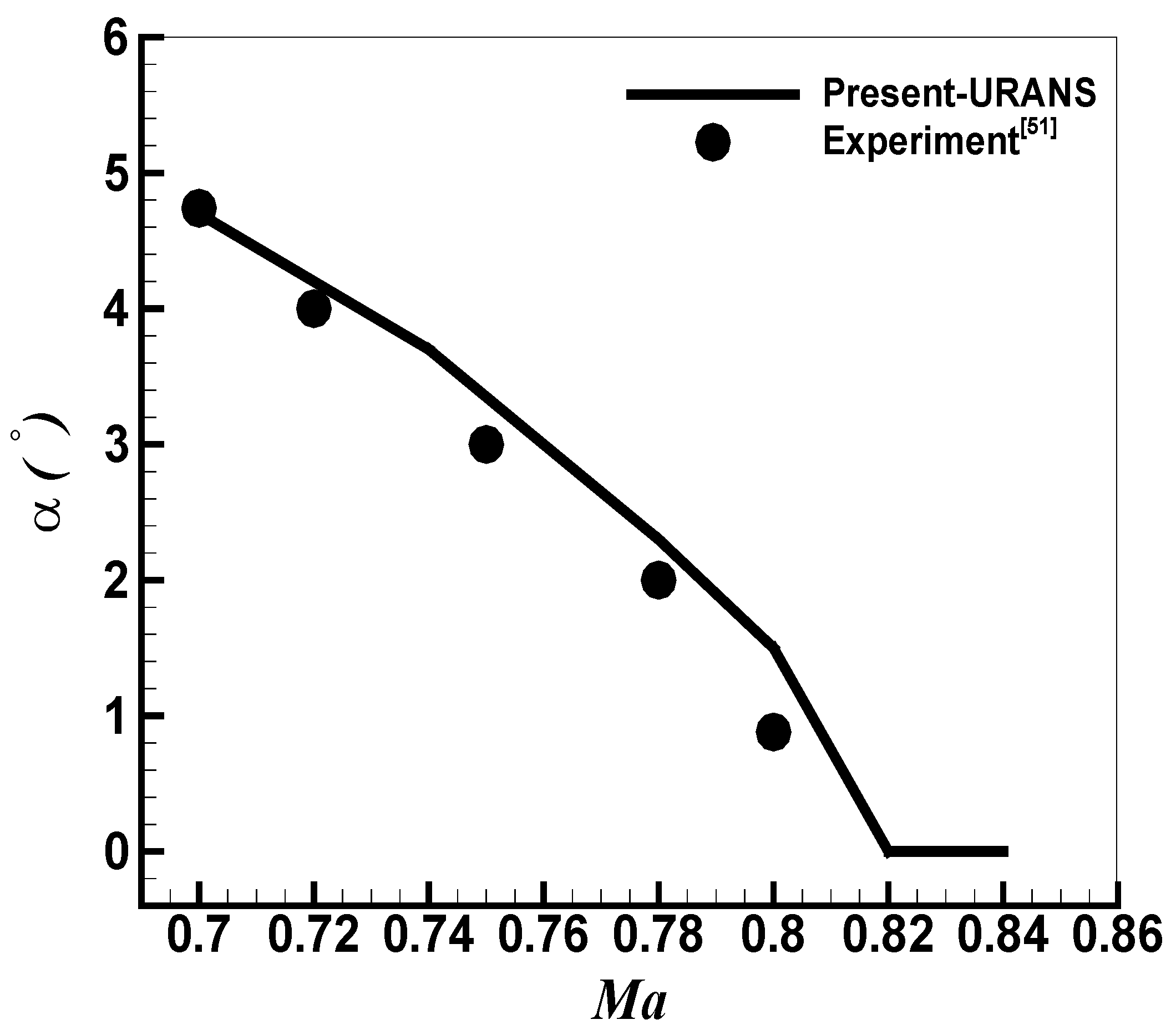
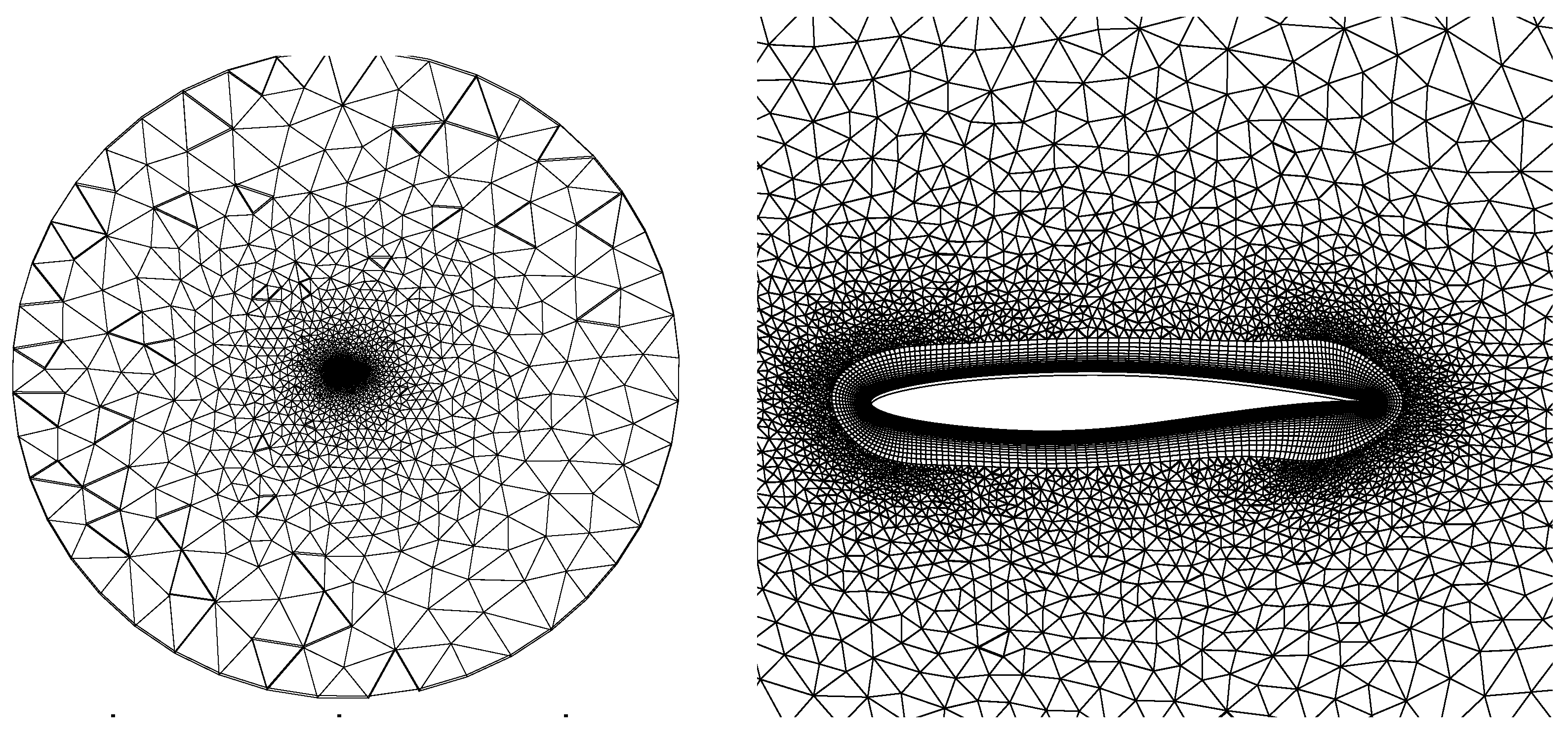
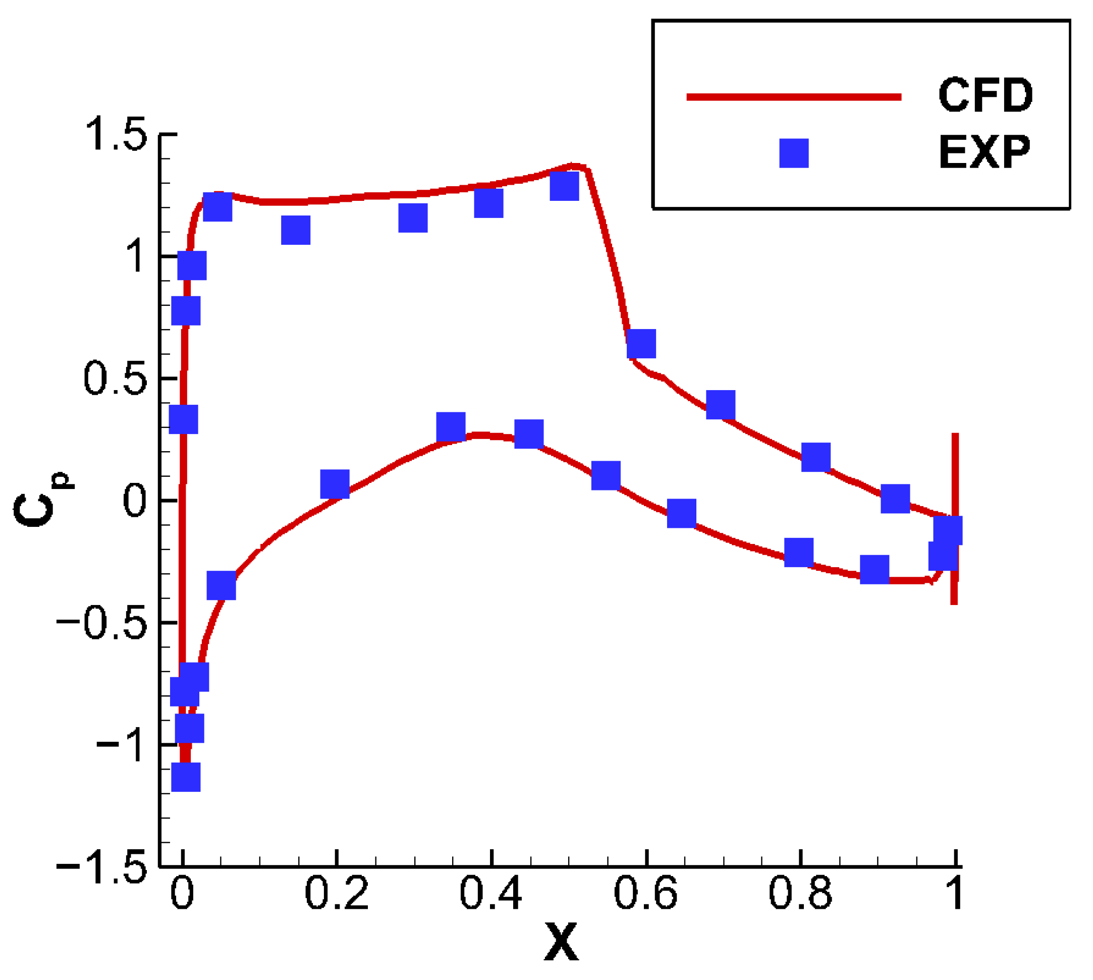
3. Numerical Method and Verification

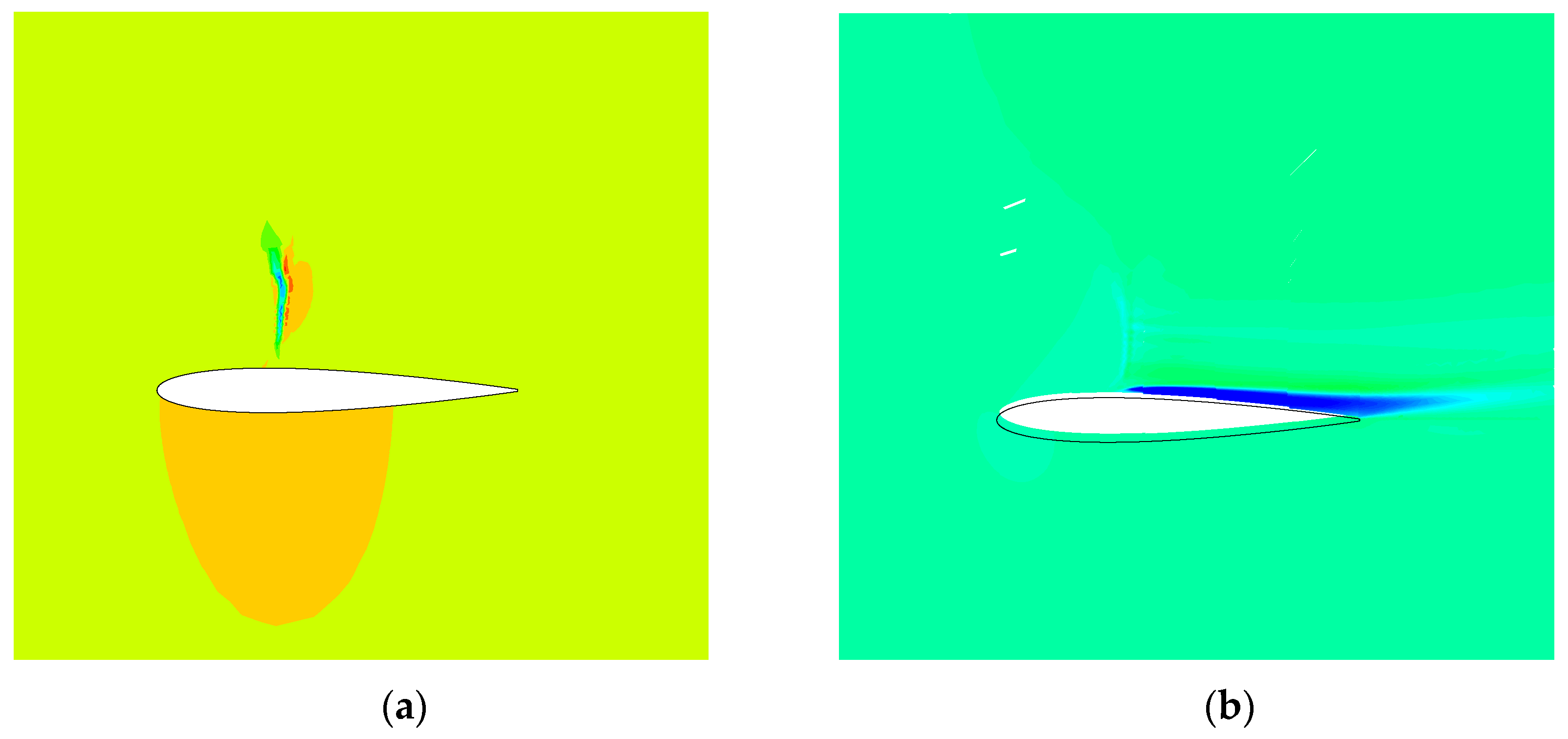
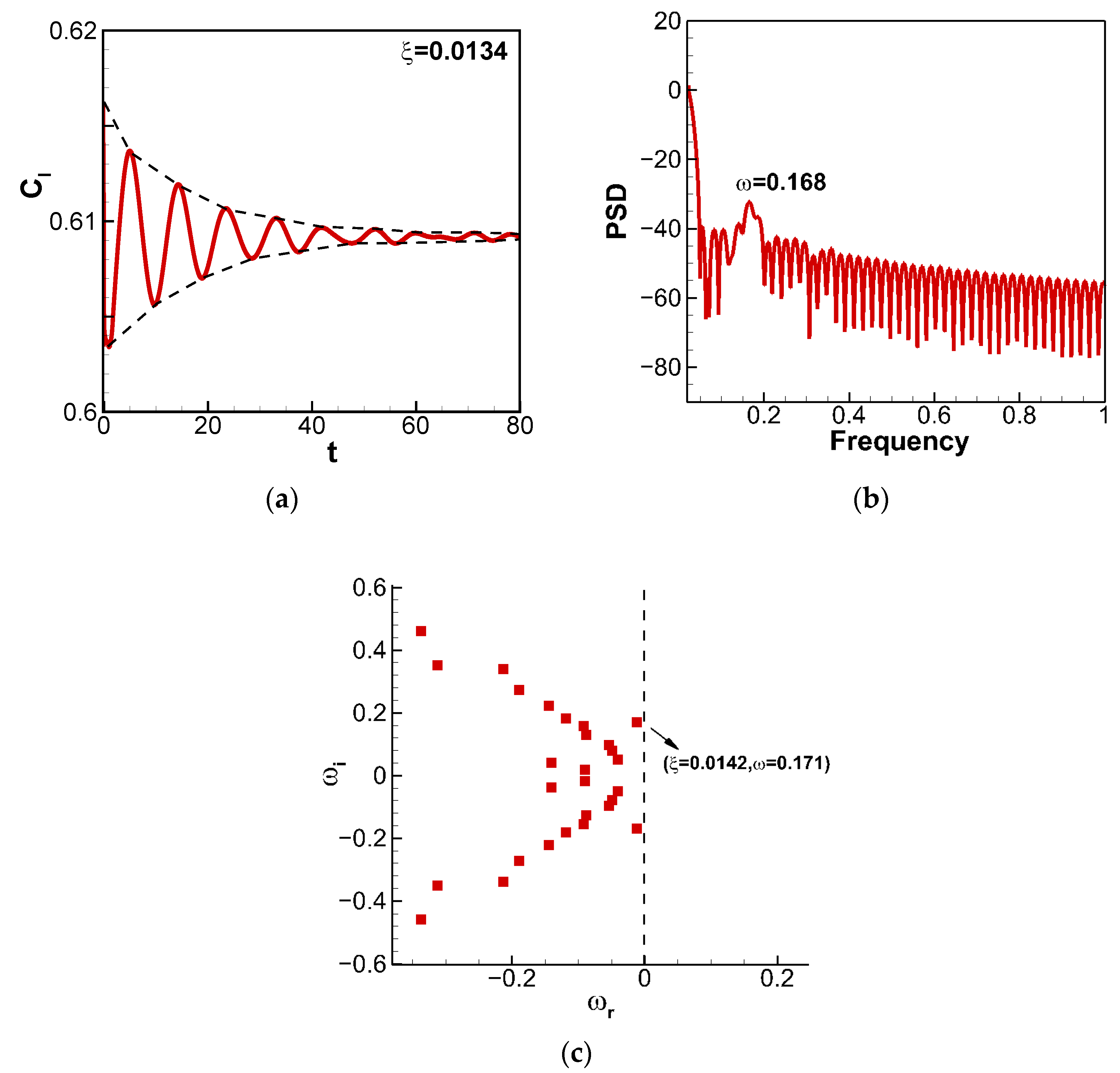
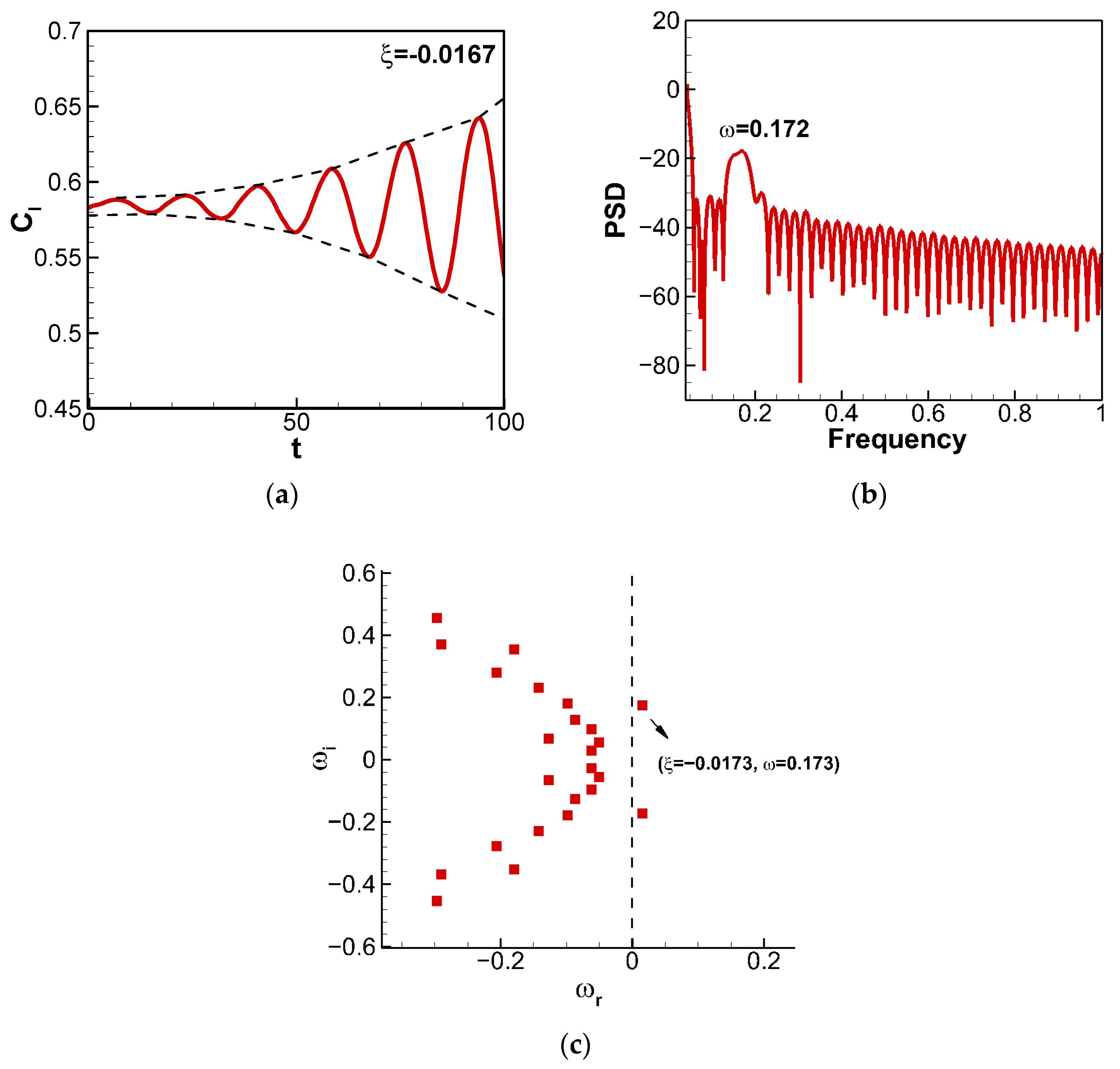
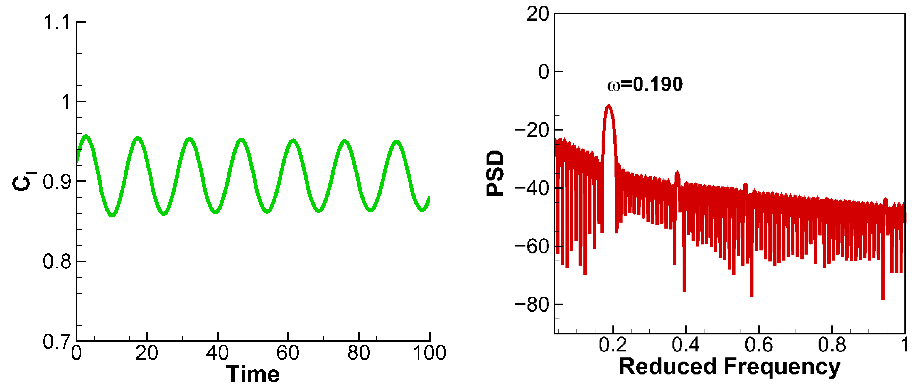
3.1. BiGlobal Stability Analysis

URANS equations are used in the numerical simulation of transonic buffet and the finite volume method is chosen as the spatial discretization method. The equations can be expressed as follows:

$$\frac{\partial }{\partial t}{\displaystyle {\iiint }_{\Omega }UdV}+{\displaystyle {\iint }_{\partial \Omega }F(U)\cdot ndS}-{\displaystyle {\iint }_{\partial \Omega }G(U)\cdot ndS}=0$$

(1)

where:

$$U=\left\{\begin{array}{c}\begin{array}{c}\rho \\ \rho u\end{array}\\ \rho v\\ e_0\\ \rho \tilde{\nu }\end{array}\right\}$$

(2)

In Equation (1), $\Omega$ is the control unit, $\partial \Omega$ is the boundary of the control unit, $n$ is the external normal of the control unit boundary, $U$ is the vector of the conservative values, $F$ is the vector of inviscid fluxes and $G$ is the vector of viscous fluxes. In Equation (2), $\left(u,v\right)$ are the flow velocity components, $\rho$ is the density, $e_0$ is the total energy and $\tilde{v}$ is the eddy-viscosity of turbulence in near-wall region. $t$ is the dimensionless time.

As a result of simplifying the URANS equations, we get Equation (3) as follows:

$$V\frac{\partial U}{\partial \mathrm{t}}=-R\left(U\right)$$

(3)

where $V$ is the diagonal matrix of control volume and $R\left(U\right)={\displaystyle {\iint }_{\partial \Omega }F\left(U\right)}·ndS-{\displaystyle {\iint }_{\partial \Omega }G\left(U\right)}·ndS$ is the vector of spatial residual. Linear analysis considers the decomposition of all flow quantities into a steady base flow $\overline{U}$ and unsteady small amplitude perturbations $\widehat{U}$ as follows:

$$U\left(X,\mathrm{t}\right)=\overline{U}\left(X\right)+\xi \widehat{U}\left(X,\mathrm{t}\right)$$

(4)

With the assumption of a small perturbation in the global instability theory, the vector of spatial residual can be written as:

$$R\left(U\right)=R\left(\overline{U}+\xi \widehat{U}\right)=R\left(\overline{U}\right)+\xi \frac{\partial R}{\partial \overline{U}}\widehat{U}$$

(5)

Substituting Equations (4) and (5) in Equation (3), the URANS equations can be written as:

$$R\left(\overline{U}\right)=0$$

(6)

$$V\frac{\partial \widehat{U}}{\partial t}=-\frac{\partial R}{\partial \overline{U}}\widehat{U}$$

(7)

where Equation (6) is the steady RANS equations and Equation (7) is the linear URANS equations of perturbation. The pseudo-time $\tau$ is introduced to solve the steady RANS equations. Equation (6) can be written as:

$$V\frac{\partial {\overline{U}}_m}{\partial \tau }=-{\overline{R}}_m$$

(8)

where ${\overline{R}}_m$ is the spatial residual of $m$th iteration. The flow outer boundary conditions are determined by Riemann reflection boundary condition, and the boundary conditions on the body surface are:

$$\left(u,v\right)=0,\tilde{\nu }=0,\frac{\partial T}{\partial n}=\frac{\partial \rho }{\partial n}=0$$

(9)

The solutions of steady RANS equations can be obtained directly if the flow is stable; but the unstable steady solutions should be solved if the flow is unstable, which is one of the difficulties in the algorithm of global stability analysis.

The main techniques to get unstable steady solutions include the selective frequency damping method [43] and feedback control method [44]. The technique of increasing the time step is used to get unstable steady solutions in this paper. Literature [45] can be referred to for details.

In the linear URANS equations of perturbation, $\widehat{U}\left(X,t\right)$ can be written in the harmonic form in the frequency domain.

$$\widehat{U}\left(X,t\right)=\tilde{U}\left(X\right)e^{-\omega t}$$

(10)

where $\omega$ are the eigenvalues in the frequency domain, $\tilde{U}$ is the amplitude of modes in the frequency domain. Substitute Equation (10) in Equation (7) results in:

$$V^{-1}\frac{\partial R}{\partial \overline{U}}\tilde{U}=\omega \tilde{U}$$

(11)

Equation (11) can also be written as:

$$A\tilde{U}=\omega \tilde{U}$$

(12)

where $A$ is the Jacobian matrix:

$$A=V^{-1}\frac{\partial R}{\partial \overline{U}}$$

(13)

As can be seen in Equation (12), the objective of the modal theory is to compute the eigenvalue decomposition of matrix $A$ which provides the eigenvalues $\omega$ and the corresponding eigenvectors $\tilde{U}$. The real part ${\omega }_r$ and the imaginary part ${\omega }_i$ of the eigenvalues $\omega$ correspond to the damping rate and the frequency of flow disturbances, respectively. The corresponding eigenvectors $\tilde{U}$ describe the mode shape, characterizing the behavior of small-amplitude flow disturbances.

Arnoldi’s algorithm [46,47] is one of the most successful approaches to solving the eigenvalue problems (EVP) of large sparse matrix $A$. It is an iterative method based on the projection of the problem on an orthogonal basis which, in this case, is a Krylov subspace. The objective is to reduce the dimension of the Jacobian matrix $A$. Then, the initial problem can be turned into solving the EVP of a much smaller projection matrix $H$. In this way, the computational costs can be largely decreased while the main eigenvalues and the corresponding eigenvectors can be obtained directly.

The Jacobian-free method is applied to the Arnoldi algorithm in order to improve the computational efficiency. Its advantage is that there is no need to store the exact Jacobian matrix. With a larger number of grid cells, its computational efficiency is more obvious. The Jacobian-free method can be expressed as follows:

$$A{v}_0=-\frac{R\left(\overline{U}+\epsilon v_0\right)-R\left(\overline{U}\right)}{\epsilon }$$

(14)

The test cases of the NACA0012 airfoil are chosen to validate the CFD solver of time-domain method and the BiGlobal analysis. A detailed wind tunnel experiment on NACA0012 transonic flutter [48] and buffet [49,50] has been conducted by the researchers. Figure 2 shows the computational grid. The total number of grid cells is 25,941 and that of nodes is 18,249. The number of nodes on the airfoil surface is 257. The height of the first boundary layer is $1\times {10}^{-5}$ times the chord length and the total height of boundary layers is 0.015 times the chord length. The Ausmup scheme is applied to perform the spatial discretization of inviscid fluxes, and the central scheme to that of viscous fluxes. The Spalart–Almaras (SA) turbulence model is employed for the turbulence solver. The generalized minimum residual method (GMRES) is selected for the Jacobian matrix solution algorithm and symmetric Gauss–Seidel (SGS) method is for the preconditioner.

The state of test cases is $Ma=0.7,\mathrm{Re}=3.0\times {10}^6$. The eigenvalues of different angles of attack are computed by the BiGlobal analysis. Figure 3 shows the comparison among the BiGlobal analysis results and URANS simulation. As shown in Figure 3, the flow frequency, damping rate of disturbance and unstable boundary computed by the BiGlobal analysis correspond well with the URANS simulation. Figure 4 and Figure 5 show the flow field and flow mode of NACA0012 airfoil, respectively, in the state of $Ma=0.7,\alpha =4.7°,\mathrm{Re}=3.0\times {10}^6$.

Figure 6 and Figure 7 show the numerical simulation in the time domain and the eigenvalues computed by the BiGlobal analysis in the states of $\alpha ={4.6}^{\circ },{4.7}^{\circ }$. The power spectrum analysis is applied to compute the frequency in the numerical simulation, and the error is within 0.5%. Flow damping is actually the opposite of the damping rate of disturbance. As can be seen in the figures, in the state of $\alpha ={4.6}^{\circ }$, the flow damping is 0.0142 and the frequency is 0.171 as computed by the BiGlobal analysis. This agrees well with the results of the numerical simulation. The error of the two methods is not over 6%. The eigenvalues are all on the left side of the zero axis and the flow damping is positive. That is, the flow field is stable. In the state of $\alpha ={4.7}^{\circ }$, the flow damping is −0.0173 and the frequency is 0.173 as computed by the BiGlobal analysis. This agrees well with the results of numerical simulation. The error between the two methods is not over 4%. There is a pair of eigenvalues crossing the zero axis, and the flow damping is negative. Namely, the flow field becomes unstable and the transonic buffet occurs. In this way, the consistency of the BiGlobal analysis and the numerical simulation in the time domain has been validated.

The buffet onsets of NACA0012 airfoil at different $Ma$ numbers are computed by the BiGlobal analysis and URANS simulation. Figure 8 compares the computational results with the experimental results [51]. As can be seen from Figure 8, the computational results correspond well with the results of the experimental results except for the case $Ma=0.80$.

RAE2822 airfoil is used for the shape optimization in this paper, so the reliability verification of the CFD solver is also tested. Figure 9 shows the computational grid of RAE2822. The total number of grid cells is 16,119 and that of nodes is 20,420. The number of nodes on the airfoil surface is 204. The height of the first boundary layer is $5\times {10}^{-6}$ times the chord length and the total height of the boundary layer is 0.1 times the chord length. CFD solver of RAE2822 remains the same.

The pressure coefficients computed by the CFD solver agree well with the experimental results, as shown in Figure 10. The CFD solver tends to over-predict the pressure in the attached boundary layer. The buffet onsets computed by the BiGlobal analysis are close to the reference results [52] shown in Figure 11. Therefore, our CFD solver of the BiGlobal analysis has been validated and, as a result, can be used in the airfoil optimization design of the buffet.

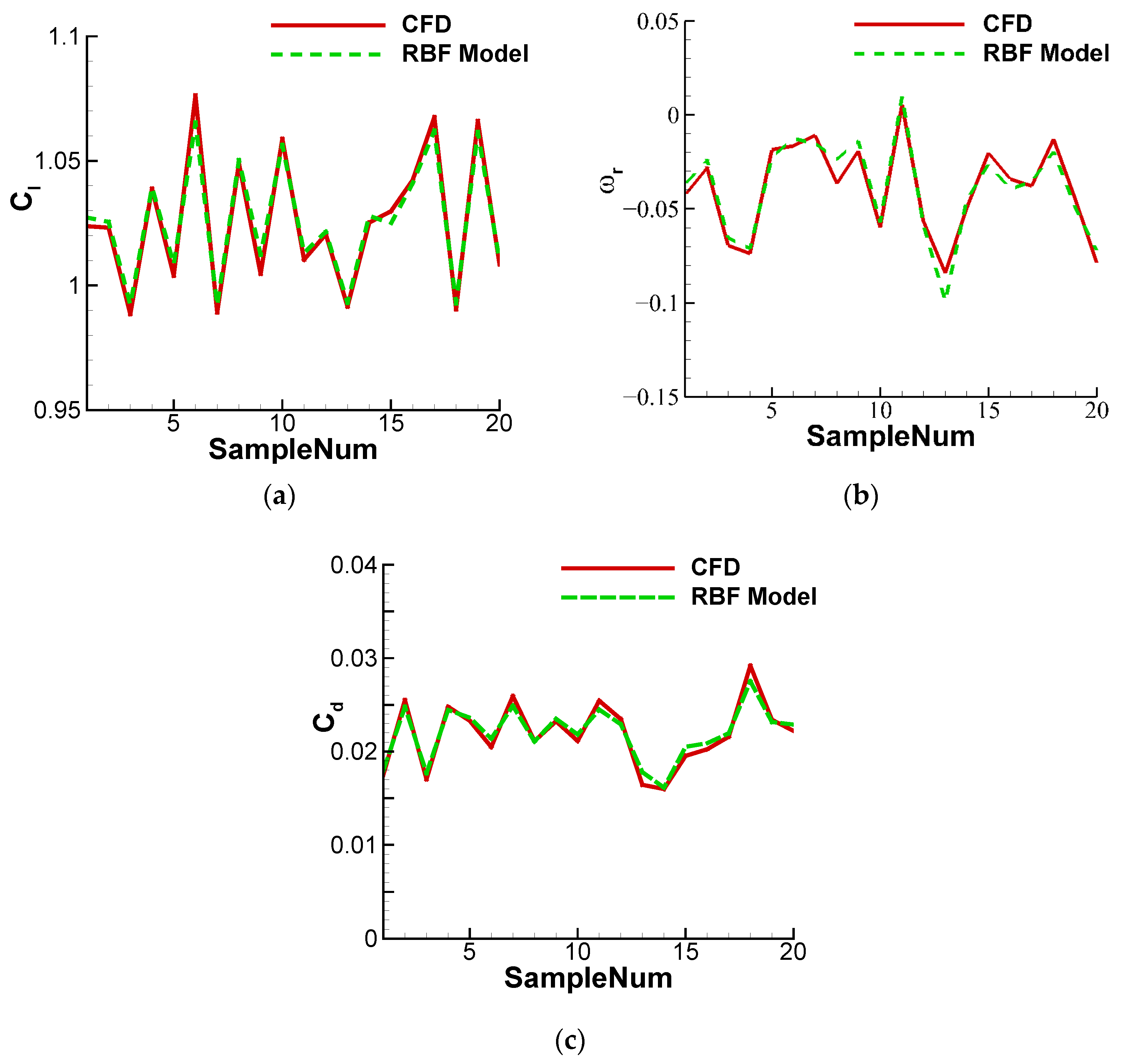
3.2. The Surrogate Model Based on the RBF Interpolation

The CFD solver should be used many times in the airfoil optimization design. However, the RBF surrogate model is often applied in the optimization process instead of the CFD solver to improve the efficiency. It has the advantages of simple data structure, high model accuracy and independence of space dimension. These make it widely researched, developed and applied in the engineering science of aerospace and automobiles.

The base form of the RBF interpolation can be expressed as:

$$F\left(x\right)={\displaystyle \sum _{i=1}^N{l}_i}\phi \left(‖x-x_i‖\right)$$

(15)

where $F\left(x\right)$ is the interpolation function, which represents the aerodynamic coefficient or the damping rate of disturbance computed by the CFD solver in this study; $N$ is the total number of radius-based functions, which represents the number of samples to construct the surrogate models; $x_i$ is the $i$th parameter vector of the airfoil in the literature; $l_i$ is the RBF weight coefficient of the $i$th sample point; and $\phi \left(‖x-x_i‖\right)$ is the radial basis function. There are various types of radius-based functions, however the Gaussian basis function is selected one in this study. It can be expressed as Equation (16):

$$\phi (\eta )=\exp (-\eta /(2{\sigma }^2))$$

(16)

where $\sigma$ is the shape parameter of the radius-based function.

To solve the weight coefficients $l={\left(l_1,l_2,\cdots ,l_N\right)}^T$, linear equations are constructed as Equation (17).

$$\Phi l=F_x$$

(17)

where $F\left(x\right)={\left(F\left(x_1\right),\cdots ,F\left(x_N\right)\right)}^T$. The specific form of matrix $\Phi$ can be expressed as Equation (18).

$$\begin{array}{l}\Phi =\left.\left\{\begin{array}{lllll}\phi (||x_1-x_1||)& \cdots & \phi (||x_1-x_j||)& \cdots & \phi (||x_1-x_N||)\\ ⋮& & ⋮& & ⋮\\ \phi (||x_j-x_1||)& \cdots & \phi (||x_j-x_j||)& \cdots & \phi (||x_j-x_N||)\\ ⋮& & ⋮& & ⋮\\ \phi (||x_N-x_1||)& \cdots & \phi (||x_N-x_j||)& \cdots & \phi (||x_N-x_N||)\end{array}\right.\right\}\\ \end{array}$$

(18)

The weight coefficients in Equation (17) can be solved by putting in the sample data. Thus, for the input parameter of an arbitrary airfoil, the output parameter of CFD results $F_x$ can be solved by solving Equation (15). This means that the CFD solver can be replaced by the RBF surrogate model.

To verify the accuracy of the RBF models, 18 CST parameters of RAE2822 are obtained by CST parameterization. One-hundred-and-fifty samples of airfoil parameters in the design space are selected by LHS to construct RBF models, the inputs of which are airfoil parameters and the outputs of which are the aerodynamic force coefficients and damping rate of disturbance. Another 20 sample points are selected for accuracy verification. The designed state is: $Ma=0.734,\alpha ={5.6}^{\circ },\mathrm{Re}=6.5\times {10}^6$. The results of accuracy verification are shown in Figure 12, and the damping rate of disturbance is solved by the BiGlobal analysis. As can be seen in the figures, the accuracy of RBF models meets the requirement of airfoil optimization.

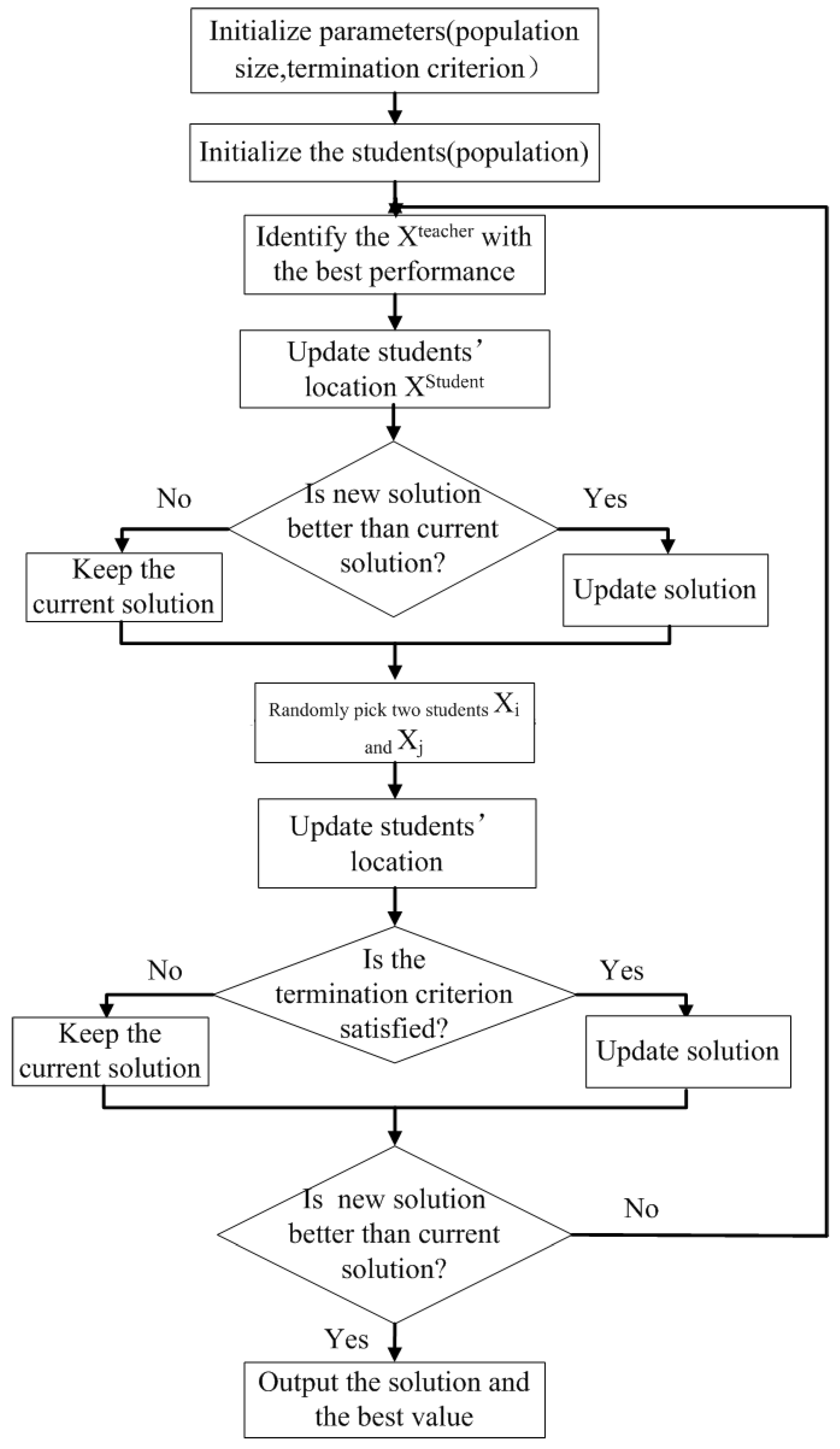
3.3. The Teaching- and Learning-Based Optimization

The TLBO algorithm is a population-optimized algorithm based on the teaching-learning pattern, which was proposed by Rao R V [53]. It has a good effect on optimization without artificial parameters and also has better search capabilities for high-dimension problems.

In the TLBO algorithm, $N_p$ initial airfoil sample points are chosen as learners. Sample $X_t$ is the teacher with the most knowledge, which means it has the minimized value of optimization function. In this paper, the damping rate of the teacher is minimized in the specified state. The main idea of the TLBO algorithm is to improve the total knowledge level of the class through teaching by the teacher and learning from each other among the learners as well. Furthermore, the knowledge of learners can give feedback to the teacher after each process of learning, and the knowledge level of the teacher is improved. Finally, the optimized solution is found in the design space when the knowledge level of the teacher reaches the saturation point.

Teaching phase is the first part of the algorithm where learners learn through the teacher. For the period of this phase, a teacher tries to increase the mean result of the class in the subject taught by him or her depending on his or her capacity. Let $M_i$ be the mean and $T_i$ be the teacher at any interaction $i$. The solution is updated by:

$$Dif\text{\_}Mea{n}_i=r_i\left(M_{new}-T_F{M}_i\right)$$

(19)

where $M_{new}$ is the results of the best learner in all sample points. $T_F$ is the teaching factor that decides the value of mean to be changed and $r_i$ is a random number in the range [0, 1]. This difference modifies the existing solution according to the following expression:

$$X_{new,i}=X_{old,i}+Dif\text{\_}Mea{n}_i$$

(20)

The learner phase is the second part of the algorithm. Learners increase their knowledge by interacting among themselves. A learner interacts randomly with other learners for increasing their knowledge and learns new things if the other learner has more knowledge than him or her. Learner modification is expressed as:

$$For\begin{array}{cc} & i=1:P_n\end{array}$$

Randomly select two learners $X_i$ and $X_j\begin{array}{cc} & \left(i\ne j\right)\end{array}$

$$\begin{gathered} if\begin{array}{cc} & f\left(X_i\right)\end{array}<f\left(X_j\right) \\ {X}_{new,i}=X_{old,i}+r_i\left(X_i-X_j\right) \\ \begin{array}{l}else\\ X_{new,i}=X_{old,i}+r_i\left(X_j-X_i\right)\\ end\begin{array}{cc} & if\end{array}\\ end\begin{array}{cc} & for\end{array}\end{array} \end{gathered}$$

This algorithm requires only the common control parameters, such as the population size and the number of generations, and does not require any algorithm-particular control parameters. Figure 13 shows the flow chart of the TLBO algorithm.

4. Airfoil Optimization

4.1. Optimization Description

Commercial aircrafts are required to have at least a 1.3 g buffet onset boundary from cruise states. In this case, the buffet onset is chosen as a constraint in the airfoil optimization. RAE2822 airfoil is chosen as the initial airfoil. The cruise state of RAE2822 is $Ma=0.734,\mathrm{Re}=6.5\times {10}^6,C_l=0.824$, which is provided by AIAA aerodynamic design optimization discussion group (ADODG) [54]. As can be seen in Figure 14, the lift coefficient of RAE2822 airfoil is 0.8247 in the state of $Ma=0.734,\alpha ={2.8}^{\circ },\mathrm{Re}=6.5\times {10}^6$. The objective is to minimize the drag coefficient ($C_d$) of the RAE2822 in the state of $Ma=0.734,\alpha ={2.8}^{\circ },\mathrm{Re}=6.5\times {10}^6$ subject to an area and pitching moment constraint in the design state.

The aerodynamic optimization is described as follows.

$$\begin{array}{c}\mathbf{Aerodynamic}\mathrm{optimization}\\ \\ \begin{array}{l}\min C_d\\ s.t. X_{\min }\le X_{design}\le X_{\max }\\ A_s\ge A_{s\text{\_}initial}\\ case\left(\alpha ={2.8}^{\circ }\right): {\overline{C}}_{ }{ }_l=0.824\\ {\overline{C}}_{ }{ }_m\ge -0.092\end{array}\end{array}$$

where $A_s$ is the area of airfoil, $A_{s\text{\_}initial}$ is the area of the initial airfoil and ${\overline{C}}_l$ and ${\overline{C}}_m$ are the time-averaged lift coefficient and moment coefficient, respectively. $X_{design}={\left[x_1,x_2,\cdots x_n\right]}^T$ is the design parameter vector of CST and $n$ is the number of parameters. $X_{\min }={\left[x_{1\min },x_{2\min },\cdots ,x_{n\min }\right]}^T$ and $X_{\max }={\left[x_{1\max },x_{2\max },\cdots ,x_{n\max }\right]}^T$ represent the lowest and highest boundary of the design space, respectively. Because the buffet occurs at $\alpha ={4.3}^{\circ }$, 1.3 times the design lift coefficient is beyond the reach. Figure 15 shows the time domain response and power spectrum analysis in the state of $Ma=0.734,\alpha ={4.8}^{\circ },\mathrm{Re}=6.5\times {10}^6$. We suppose that the lift coefficient curve is linear after $\alpha =3^{\circ }$, then the 1.3 times the design lift coefficient is reachable in the state of $\alpha ={5.6}^{\circ }$. We intend to delay the buffet onset so that the optimized airfoil can be reached 1.3 times the design lift coefficient in the state of $Ma=0.734,\alpha ={5.6}^{\circ },\mathrm{Re}=6.5\times {10}^6$ without a buffet.

Based on the aerodynamic optimization, the constraint of 1.3 times the design lift coefficient without buffet in the state of $Ma=0.734,\alpha ={5.6}^{\circ },\mathrm{Re}=6.5\times {10}^6$ is added. The damping rate of flow disturbance ${\omega }_r$ can indicate the flow stability, which has been proven before. As a result, ${\omega }_r$ is selected as the constraint variable of the optimization. The mathematical model of the aerodynamic optimization considering buffet suppression is shown as follows.

$$\begin{array}{c}\mathbf{Aerodynamic}\mathbf{optimization}\mathbf{considering}\mathbf{buffet}\mathbf{suppression}\\ \\ \begin{array}{c}\min C_d\\ s.t. X_{\min }\le X_{design}\le X_{\max }\\ A_s\ge A_{s\text{\_}initial}\\ case\left(\alpha ={2.8}^{\circ }\right): {\overline{C}}_{ }{ }_l=0.824\\ \begin{array}{cc}\begin{array}{cc} & \end{array}& {\overline{C}}_{ }{ }_m\ge -0.092\end{array}\hfill \\ case\left(\alpha ={5.6}^{\circ }\right): {\omega }_R<0\\ {\overline{C}}_l>1.07\end{array}\end{array}$$

The CST parameterization method can describe an arbitrary airfoil by fewer parameters and has a stronger ability of transformation, therefore it is selected for the airfoil parameterization. A total of 18 CST parameters of RAE2822 are obtained by CST Parameterization. The design space is within the range of 35% of the 18 parameters. The RBF surrogate models are used to replace the CFD solver, in which the CST airfoil parameters are chosen as the inputs and the time-average aerodynamic coefficients and the damping rate of disturbance ${\omega }_r$ are chosen as the outputs. A total of 150 samples of airfoil parameters in the design space are selected by LHS to construct RBF models. The prior probability distribution of the parameters is uniform. Another 20 sample points are selected for accuracy verification. The accuracy of the RBF model is verified in Section 3.2. The TLBO algorithm is used for the optimization.

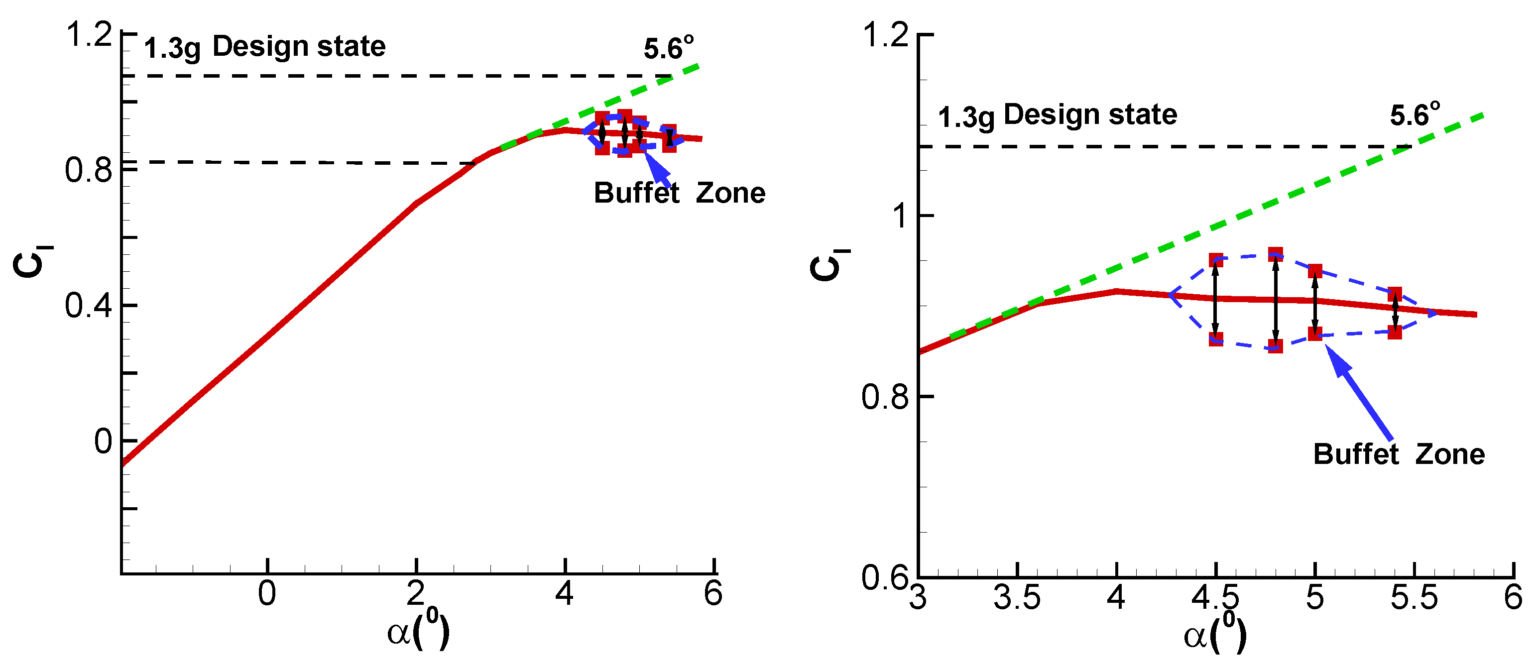
4.2. Optimization Results and Analysis

In aerodynamic optimization, the optimized value converges at 0.01306 through 500 generations. The optimized airfoil is named “Opt_1”. In Figure 16 and

Table 1. RAE2822 optimization and comparison with other benchmark results.

Airfoil	${\overline{\mathit{C}}}_{\mathit{l}}$	$\mathbf{Opt}\text{\_}{\overline{\mathit{C}}}_{\mathit{d}}$	$\mathbf{Base}\text{\_}{\overline{\mathit{C}}}_{\mathit{d}}$	$\mathbf{\Delta }{\overline{\mathit{C}}}_{\mathit{d}}$	${\mathit{C}}_{\mathit{l}}/{\mathit{C}}_{\mathit{d}}$
RAE2822	0.8247	0.02079	0.02079	0%	39.75
Optimize_1	0.8252	0.01306	0.02079	−37%	63.17
Optimize_2	0.8248	0.01387	0.02079	−33%	59.46
Ref_Leifsson [55]	0.8246	0.01270	0.01652	−23%	64.93
Ref_Lee [56]	0.8239	0.01314	0.02340	−44%	62.70
Ref_Wu [57]	0.8241	0.01129	0.01953	−42%	72.98

, the present optimization achievements are compared to selected results obtained by other research groups on the same benchmark case. It is proven that the aerodynamic optimization benchmark in this paper has good performance. The upper surface shape of the optimized airfoil in this paper is similar with the benchmark results. There are three obvious characteristics of the optimized airfoils compared to the initial airfoil: (1) the curvature of the leading edge decreases and the curvature of the trailing edge increases on the upper surface, (2) the maximum thickness position of the upper surface moves backward to about 0.53c and (3) the curvature of the leading edge on the lower surface increases in order to improve the camber of the airfoil. In this work, the drag reduction is 37% and the lift-drag ratio increases by 58.9% after optimization. Therefore, the validation of optimized shape and optimization methods in this paper has been performed.

Figure 17 shows a comparison of optimized $C_p$ distribution by other international counterparts. It can be observed that the intensity of the shock wave of the present study is weaker, and the position of the shock wave moves backwards after optimization. The optimized airfoil computed by Wu has the best optimization effect. For this optimized airfoil, the curvature of the leading edge on the lower surface is the maximum among all the optimized airfoils.

The 1.3 g buffet onset boundary from cruise states is used as a constraint in the second optimization. In this case, the optimized value converged at 0.01387. Figure 18 shows the convergence history of the optimization object. The optimized airfoil is named “Opt_2”.

The two optimized airfoils are compared in Figure 19. These airfoils have similar configurations in the lower surface. For the “Opt_2” airfoil, the curvature of the leading edge on the upper surface is larger and the maximum thickness position moves forward compared to the “Opt_1” airfoil.

Table 2. Comparison of two optimization results.

Airfoil	Cruise State			1.3 g Cruise State
	${\mathit{C}}_{\mathit{l}}$	${\mathit{C}}_{\mathit{d}}$	${\mathit{C}}_{\mathit{l}}/{\mathit{C}}_{\mathit{d}}$	${\overline{\mathit{C}}}_{\mathit{l}}$	${\mathit{\omega }}_{\mathit{r}}$
RAE2822	0.8247	0.02079	39.75	0.9152	−0.02609
Optimize_2	0.8248	0.01387	59.46	1.0714	−0.01173
Optimize_1	0.8252	0.01306	63.17	0.9784	0.03704
Optimize_Wu	0.8241	0.01245	66.19	0.9905	0.06714

compares the two optimization achievements in this paper. The optimized airfoil in [57], which has the best aerodynamic performance in the design state, is also added to test its flow stability at higher angles of attack. This airfoil is named “Opt_Wu”. For the “Opt_2” airfoil, the aerodynamic performance in the design state is not as good as the other two optimized airfoils. The lift-drag ratio is increased by 49.6%, lower than 58.9% in the first optimization. However, in the state of $\alpha ={5.6}^{\circ }$, the time-averaged lift coefficient of the “Opt_2” airfoil could reach 1.3 times the design lift coefficient, which is much larger than the other three airfoils. For the other three airfoils, the buffet occurs before the state of $\alpha ={5.6}^{\circ }$. The state of $\alpha ={5.6}^{\circ }$ is called the 1.3 g design state for convenience.

The pressure coefficient before and after optimization in the design state and in 1.3 g design state are shown in Figure 20 and Figure 21, respectively. In the design state, the shock wave is almost eliminated for the airfoil optimized by Wu. While there are two weak shock waves for the “Opt_2” airfoil, the drag coefficient of the “Opt_2” airfoil is higher than the other optimized airfoils. In the 1.3 g design state, the positions of the shock waves move backwards after optimization, and the shock wave is fully rearward for the “Opt_2” airfoil. Compared to the other optimized airfoils, the aerodynamic performance and flow stability of “Opt_2” airfoil on higher angle of attack is improved at the cost of decreasing the aerodynamic performance in the design state. There is still 50% improvement in the lift-drag ratio for the “Opt_2” airfoil, showing good optimization results in the design state.

The flow fields in the design state and 1.3 g design state are shown in Figure 22 and Figure 23, respectively. In the 1.3 g design state, the separated region diminishes and the position of the shock wave moves backwards after the aerodynamic optimization considering buffet suppression. Thus, the buffet onset and the maximum lift coefficient are improved for the “Opt_2” airfoil.

The lift coefficient and lift-drag curves are shown in Figure 24. The lift coefficient curves of three optimized airfoils are similar before $\alpha ={4.0}^{\circ }$, however, the lift coefficients of the airfoils are no longer growing after $\alpha ={4.5}^{\circ }$ except for the “Opt_2” airfoil. The maximum lift coefficient of “Opt_2” airfoil is at least 9% larger than other optimized airfoils. The maximum lift-drag ratio of “Opt_2” airfoil is at $\alpha ={3.0}^{\circ }$, which is ${0.2}^{\circ }$ larger than the design state. Therefore, there are two weak shock waves in the design state. The maximum lift-drag ratio of “Opt_Wu” airfoil is larger than other optimized airfoils, but as the angle of attack increases, the lift-drag ratio of “Opt_2” airfoil becomes the maximum after $\alpha ={4.0}^{\circ }$. Therefore, the aerodynamic performance at a higher angle of attack is improved and 1.3 times the design lift coefficient can be reached after the aerodynamic optimization considering buffet suppression.

The damping rate of disturbance and the buffet amplitude of these four airfoils after $\alpha ={4.0}^{\circ }$ are shown in Figure 25. There are obvious improvements both in the stability margin and aerodynamic performance after the aerodynamic optimization considering buffet suppression. The buffet onset angle of attack is increased by 1.5° and the maximum lift coefficient is increased by 15.7%. Meanwhile, the instability region is decreased by 37.5% and the maximum buffet amplitude is decreased by 17%. If the buffet onset is not considered in the optimization, there is no significant improvement in stability margin. For the “Opt_1” airfoil and the “Opt_Wu” airfoil, the buffet onset angle of attacks are increased by about 0.5° but the instability regions and the maximum buffet amplitudes are larger than the RAE2822 airfoil. Buffet occurs before the 1.3 times the design lift coefficient is reached. The time histories of the lift coefficient in the state of $\alpha ={5.4}^{\mathrm{o}}$ and ${5.6}^{\mathrm{o}}$ are shown in Figure 26, which verifies our viewpoints above. The buffet onset should be considered in the shape optimization to satisfy the requirements of aerospace engineering.

5. Conclusions

Buffet has a strong influence on transonic aviation. A 1.3 times of maneuver overload in cruise flight without a buffet is needed in aerospace engineering. However, the buffet suppression is not considered in most of the airfoil optimization design. Therefore, in this paper, a transonic buffet suppression methodology by the airfoil optimization based on the global stability analysis is proposed. The damping rate of disturbance, computed by the BiGlobal analysis, can be used to represent the characteristics of the flow stability. The objective of our study is to optimize airfoils in terms of aerodynamic performance and flow stability. There is no buffet in the 1.3 g maneuver in cruise flight after optimization.

RAE2822 airfoil is chosen as the initial airfoil. The damping rate of disturbance is chosen as a constraint of the shape optimization to satisfy the requirement of buffet suppression. For the upper surface of the optimized airfoils, the maximum thickness position of the airfoil moved backward, the curvature of the leading edge decreased and the trailing edge increased. There are significant improvements in buffet onset and maximum lift coefficient after the aerodynamic optimization considering buffet suppression. The lift-drag ratio of “Opt_2” airfoil is increased by about 50% in the design state. The “Opt_2” airfoil has a 1.3 g buffet onset boundary from cruise states, which meets the requirements of aerospace engineering. Compared to the initial airfoil, the buffet onset angle of attack is increased by 1.5° and the maximum lift coefficient is increased by 15.7%. Meanwhile, the instability region is decreased by 37.5% and the maximum buffet amplitude is decreased by 17%, which shows a good effect of the optimization proposed in this paper.

If the buffet onset is not considered in the shape optimization, there is no significant improvement in the stability margin. The buffet occurs at a lower angle of attack and the 1.3 times the design lift coefficient cannot be reached. Compared to these optimized airfoils, the aerodynamic performance and flow stability of “Opt_2” airfoil on higher angle of attack is improved with the cost of decreasing the lift-drag ratio in the design state to a certain extent. This paper shows the importance of considering the buffet onset in the airfoil optimization and outlines how to achieve it.

References

1. Lee, B.H.K.; Murty, H.; Jiang, H. Role of Kutta waves on oscillatory shock motion on an airfoil. AIAA J. 1994, 32, 789–796. [Google Scholar] [CrossRef]
2. Raghunathan, S.; Early, J.; Tulita, C. Periodic transonic flow and control. Aeronaut. J. 2008, 112, 1–16. [Google Scholar] [CrossRef]
3. Ogawa, H.; Babinsky, H.; Pätzold, M.; Lutz, T. Shock-wave/boundary-layer interaction control using three-dimensional bumps for transonic wings. AIAA J. 2008, 46, 1442–1452. [Google Scholar] [CrossRef]
4. Tian, Y.; Liu, P.; Li, Z. Multi-objective optimization of shock control bump on a supercritical wing. Sci. China-Tech. Sci 2014, 57, 192–202. [Google Scholar] [CrossRef]
5. Mayer, R.; Lutz, T.; Kramer, E. Control of transonic buffet by shock control bumps on wing-body configuration. J. Aircr. 2019, 56, 556–568. [Google Scholar] [CrossRef]
6. Caruana, D.; Mignosi, A.; Corrège, M.; Le Pourhiet, A.; Rodde, A. Buffet and buffeting control in transonic flow. Aerosp. Sci. Technol. 2005, 9, 605–616. [Google Scholar] [CrossRef]
7. Tian, Y.; Li, Z.; Liu, P. Upper Trailing-Edge Flap for Transonic Buffet Control. J. Aircr. 2018, 55, 382–389. [Google Scholar] [CrossRef]
8. Mabey, D.G. Oscillatory Flows from Shock Induced Separations on Biconvex Aerofoils of Varying Thickness in Ventilated Wind Tunnels, Boundary Layer Effects on Unsteady Airloads; Advisory Group for Aerospace Research and Development TR 296: Aix-en-Provence, France, 1981. [Google Scholar]
9. Jiang, R.; Tian, Y.; Liu, P. Transonic buffet control by rearward buffet breather on supercritical airfoil and wing. Aerosp. Sci. Technol. 2019, 89, 204–219. [Google Scholar] [CrossRef]
10. Zhou, H. Numerical analysis of effect of mini-TED on aerodynamic characteristic of airfoils in transonic flow. Acta Aeronaut. Astronaut. Sin. 2009, 30, 1367–1373. [Google Scholar]
11. Sartor, F.; Minervino, M.; Wild, J.; Wallin, S.; Maseland, H.; Dandois, J. A CFD benchmark of active flow control for buffet prevention. CEAS Aeronaut. J. 2019, 11, 837–847. [Google Scholar] [CrossRef]
12. Siauw, W.; Bonnet, J.-P.; Tensi, J.; Cordier, L.; Noack, B.; Cattafesta, L. Transient dynamics of the flow around a NACA 0015 airfoil using fluidic vortex generators. Int. J. Heat Fluid Flow 2010, 31, 450–459. [Google Scholar] [CrossRef]
13. Gao, C.; Zhang, W.; Ye, Z. Numerical study on closed-loop control of transonic buffet suppression by trailing edge flap. Comput. Fluids 2016, 132, 32–45. [Google Scholar] [CrossRef]
14. Zhang, K.-S.; Han, Z.-H.; Li, W.-J.; Song, W.-P. Bilevel adaptive weighted sum method for multidisciplinary multi-objective optimization. AIAA J. 2008, 46, 2611–2622. [Google Scholar] [CrossRef]
15. Leifsson, L.; Koziel, S. Aerodynamic shape optimization by variable-fidelity computational fluid dynamics models: A review of recent progress. J. Comput. Sci. 2015, 10, 45–54. [Google Scholar] [CrossRef]
16. Kenway, G.K.; Martins, J.R. Buffet-onset constraint formulation for aerodynamic shape optimization. AIAA J. 2017, 55, 1930–1947. [Google Scholar] [CrossRef]
17. Thomas, J.P.; Dowell, E.H. Discrete adjoint design optimization approach for increasing transonic buffet onset angle-of-attack. In Proceedings of the 16th AIAA/ISSMO Multidisciplinary Analysis and Optimization Conference, Dallas, TX, USA, 22–26 June 2015. [Google Scholar]
18. Thomas, J.P.; Dowell, E.H. Discrete adjoint constrained design optimization approach for unsteady transonic aeroelasticity and buffet. In Proceedings of the AIAA AVIATION 2020 FORUM, Virtual Event, 15–19 June 2020. [Google Scholar]
19. Xu, Z.; Joseph, H.S.; Yang, V. Optimization of supercritical airfoil design with buffet effect. AIAA J. 2019, 57, 4343–4353. [Google Scholar] [CrossRef]
20. Chen, H.; Gao, C.; Wu, J.; Ren, K.; Zhang, W. Study on optimization design of airfoil transonic buffet with reinforcement learning method. Aerospace 2023, 10, 486. [Google Scholar] [CrossRef]
21. Chen, W.; Gao, C.; Zhang, W.; Gong, Y. Adjoint-based unsteady shape optimization to suppress transonic buffet. Aerosp. Sci. Technol. 2022, 127, 107668. [Google Scholar] [CrossRef]
22. Iovnovich, M.; Raveh, D.E. Transonic unsteady aerodynamics in the vicinity of shock-buffet instability. J. Fluid Struct. 2012, 29, 131–142. [Google Scholar] [CrossRef]
23. Deck, S. Numerical simulation of transonic buffet over a supercritical airfoil. AIAA J. 2005, 43, 1556–1566. [Google Scholar] [CrossRef]
24. Garnier, E.; Deck, S. Large-eddy simulation of transonic buffet over a supercritical airfoil. In Turbulence and Interactions; Springer: Berlin/Heidelberg, Germany, 2010; pp. 135–141. [Google Scholar]
25. Sengupta, T.K.; Bhole, A.; Sreejith, N.A. Direct numerical simulation of 2D transonic flows around airfoils. Comput. Fluids 2013, 88, 19–37. [Google Scholar] [CrossRef]
26. Li, Q.; Cao, X.L.; Liu, Y.; Wang, G. Numerical research on the transonic buffet loads of a supercritical airfoil. Tactical Missile Technol. 2018, 38, 44–51. [Google Scholar]
27. Lipanov, A.M.; Karskanov, S.A. Direct numerical simulation of aerodynamic flows based on integration of the Navier—Stokes equations. Russ. J. Nonlinear Dyn. 2022, 18, 349–365. [Google Scholar] [CrossRef]
28. Chen, R.; Tsay, R.S. Nonlinear additive ARX model. J. Am. Stat. Assoc. 1993, 88, 955–967. [Google Scholar] [CrossRef]
29. Hall, K.C.; Dowell, E.H.; Thomas, J.P. Proper orthogonal decomposition technique for transonic unsteady aerodynamic flows. AIAA J. 2000, 38, 1852–1862. [Google Scholar] [CrossRef]
30. Amsallem, D.; Farhat, C. Interepolation mthod for adapting reduced-order models and application to aeroelasticity. AIAA J. 2008, 46, 1803–1813. [Google Scholar] [CrossRef]
31. He, G.; Wang, J.; Pan, C. Initial growth of a disturbance in a boundary layer influenced by a circular cylinder wake. J. Fluid Mech. 2013, 718, 116–130. [Google Scholar] [CrossRef]
32. Pierrehumbert, R.T.; Widnall, S.E. The two- and three-dimensional instabilities of a spatially periodic shear layer. J. Fluid Mech. 1982, 114, 59–82. [Google Scholar] [CrossRef]
33. Jackson, C. A finite-element study of the onset of vortex shedding in flow past variously shaped bodies. J. Fluid Mech. 1987, 182, 23–45. [Google Scholar] [CrossRef]
34. Iorio, M.C.; Gonzalez, L.M.; Ferrer, E. Direct and adjoint global stability analysis of turbulent transonic flows over a NACA0012 profile. Int. J. Numer. Methods Fluids 2015, 76, 147–168. [Google Scholar] [CrossRef]
35. Iorio, M.C.; Gonzalez, L.M.; Martínez-Cava, A. Global stability analysis of a compressible turbulent flow around a high-lift configuration. AIAA J. 2016, 54, 373–385. [Google Scholar] [CrossRef]
36. Crouch, J.D.; Garbaruk, A.; Magidov, D. Predicting the onset of flow unsteadiness based on global instability. J. Comput. Phys. 2007, 224, 924–940. [Google Scholar] [CrossRef]
37. Crouch, J.D.; Garbaruk, A.; Magidov, D.; Travin, A. Origin of transonic buffet on aerofoils. J. Fluid Mech. 2009, 628, 357–369. [Google Scholar] [CrossRef]
38. Sartor, F.; Mettot, C.; Sipp, D. Stability, receptivity, and sensitivity analysis of buffet transonic flow over a profile. AIAA J. 2015, 53, 1980–1993. [Google Scholar] [CrossRef]
39. Theofilis, V. Advances in global linear instability analysis of nonparallel and three-dimensional flows. Prog. Aerosp. Sci. 2003, 39, 249–315. [Google Scholar] [CrossRef]
40. Theofilis, V. Global linear instability. Annu. Rev. Fluid Mech. 2011, 43, 319–352. [Google Scholar] [CrossRef]
41. Gomez, F.; Gomez, R.; Theofilis, V. On three-dimensional global linear instability analysis of flows with standard aerodynamics codes. Aerosp. Sci. Technol. 2014, 32, 223–234. [Google Scholar] [CrossRef]
42. Bagheri, S.; Schlatter, P.; Schmid, P.J.; Henningson, D.S. Global stability of a jet in crossflow. J. Fluid Mech. 2009, 624, 33–44. [Google Scholar] [CrossRef]
43. Åkervik, E.; Brandt, L.; Henningson, D.S.; Hœpffner, J.; Marxen, O.; Schlatter, P. Steady solution of the Navier-Stokes equations by selective frequency damping. Phys. Fluids 2006, 18, 068102. [Google Scholar] [CrossRef]
44. Illingworth, S.J.; Morgans, A.S.; Rowley, C.W. Feedback control of cavity flow oscillations using simple linear models. J. Fluid Mech. 2012, 709, 223–248. [Google Scholar] [CrossRef]
45. Zhang, W.; Liu, Y.; Li, J. A simple strategy for capturing the unstable steady solution of an unsteady flow. Open J. Fluid Dyn. 2015, 5, 188–198. [Google Scholar] [CrossRef]
46. Arnoldi, W. The principle of minimized iterations in the solution of the matrix eigenvalue problem. Q. Appl. Math. 1951, 9, 17–29. [Google Scholar] [CrossRef]
47. Saad, Y. Variation of Arnoldi’s method for computing eigenelements of large unsymmetric matrices. Linear Algebra Appl. 1980, 34, 269–295. [Google Scholar] [CrossRef]
48. Rivera, J.A., Jr.; Dansberry, B.; Bennett, R.; Durham, M.; Silva, W. NACA0012 benchmark model experimental flutter results with unsteady pressure distributions. In Proceedings of the 33rd Structures, Structural Dynamics and Materials Conference, Dallas, TX, USA, 13–15 April 1992; p. 107581. [Google Scholar]
49. McDevitt, J.B.; Okuno, A.F. Static and Dynamic Pressure Measurements on a NACA0012 Airfoil in the Ames High Reynolds Number Facility; NASA TP-2485; National Aeronautics and Space Administration: Reston, VA, USA, 1985. [Google Scholar]
50. Doerffer, P.; Hirsch, C.; Dussauge, J.P.; Babinsky, H.; Barakos, G.N.; Doerffer, P.; Hirsch, C.; Dussauge, J.P.; Babinsky, H.; Barakos, G.N. NACA0012 with aileron(Marianna Braza). In Unsteady Effects of Shock Wave Induced Separation; Springer: Berlin/Heidelberg, Germany, 2011; pp. 101–131. [Google Scholar]
51. Soda, A.; Voss, R. Analysis of Transonic Aerodynamic Interference in the Wing-Nacelle Region for a Generic Transport Aircraft; IFASD: Munich, Germany, 2005. [Google Scholar]
52. Tian, Y.; Gao, S.; Liu, P.; Wang, J. Transonic buffet control research with two types of shock control bump based on RAE2822 airfoil. Chin. J. Aeronaut. 2017, 30, 1681–1696. [Google Scholar] [CrossRef]
53. Rao, R.V.; Savsani, V.J.; Vakharia, D.P. Teaching-learning-based optimization algorithm for unconstrained and constrained real-parameter optimization problems. Eng. Optim. 2012, 44, 1447–1462. [Google Scholar] [CrossRef]
54. Lane, K.A.; Marshall, D.D. Inverse airfoil design utilizing CST parameterization. In Proceedings of the 48th AIAA Aerospace Sciences Meeting Including the New Horizons Forum and Aerospace Exposition, Orlando, FL, USA, 4–7 January 2010; pp. 1228–1242. [Google Scholar]
55. Leifsson, L.T.; Koziel, S.; Hosder, S. Aerodynamic design optimization: Physics-based surrogate approaches for airfoil and wing design. In Proceedings of the 52nd Aerospace Sciences Meeting, National Harbor, MD, USA, 13–17 January 2014. [Google Scholar]
56. Lee, C.; Koo, D.; Telidetzki, K.; Buckley, H.; Gagnon, H.; Zingg, D.W. Aerodynamic shape optimization of benchmark problems using Jetstream. In Proceedings of the 53rd Aerospace Science Meeting, Kissimmee, FL, USA, 5–9 January 2015. [Google Scholar]
57. Wu, X.; Zhang, W.; Peng, X.; Wang, Z. Benchmark aerodynamic shape optimization with the POD-based CST airfoil parametric method. Aerosp. Sci. Technol. 2019, 84, 632–640. [Google Scholar] [CrossRef]
Figure 1. Optimization framework.
Aerospace 11 00121 g001
Figure 2. Computational grids for NACA0012 airfoil.
Aerospace 11 00121 g002
Figure 3. Mode eigenvalues of different angles of attack.
Aerospace 11 00121 g003
Figure 4. Flow field of NACA0012 airfoil. (a) Pressure, (b) horizontal velocity.
Aerospace 11 00121 g004
Figure 5. Unstable mode of pressure perturbation. (a) Pressure perturbation, (b) horizontal velocity perturbation.
Aerospace 11 00121 g005
Figure 6. Numerical simulation and global stability analysis in the state of α = 4.6 . (a) Time domain response, (b) power spectrum analysis, (c) eigenvalues computed by BiGlobal analysis.
Aerospace 11 00121 g006
Figure 7. Numerical simulation and global stability analysis in the state of α = 4.7 . (a) Time domain response, (b) power spectrum analysis, (c) eigenvalues computed by BiGlobal analysis.
Aerospace 11 00121 g007
Figure 8. Transonic buffet onset of NACA0012 airfoil.
Aerospace 11 00121 g008
Figure 9. Computational grids for the RAE2822 airfoil.
Aerospace 11 00121 g009
Figure 10. Pressure coefficients in state of M a = 0.73 , α = 3.19 , Re = 6.5 × 10 6 .
Aerospace 11 00121 g010
Figure 11. Critical lift coefficient and angle of attack at buffet boundary.
Aerospace 11 00121 g011
Figure 12. Accuracy verification of RBF models in the state of M a = 0.734 , Re = 6.5 × 10 6 , α = 5.6 . (a) Lift coefficient accuracy verification, (b) damping rate accuracy verification, (c) drag coefficient accuracy verification.
Aerospace 11 00121 g012
Figure 13. The flow chart of the TLBO algorithm.
Aerospace 11 00121 g013
Figure 14. Lift coefficient of RAE2822 airfoil.
Aerospace 11 00121 g014
Figure 15. Time-domain response and power spectral density of RAE2822 airfoil in the state of M a = 0.734 , α = 4.8 , Re = 6.5 × 10 6 .
Aerospace 11 00121 g015
Figure 16. RAE2822 optimization and comparison with other benchmark optimized airfoil results.
Aerospace 11 00121 g016
Figure 17. Pressure coefficient results in the design state.
Aerospace 11 00121 g017
Figure 18. Convergence history of the airfoil optimization.
Aerospace 11 00121 g018
Figure 19. Configuration of two optimized airfoils.
Aerospace 11 00121 g019
Figure 20. Pressure coefficient in the design state.
Aerospace 11 00121 g020
Figure 21. Pressure coefficient in the 1.3 g design state.
Aerospace 11 00121 g021
Figure 22. Pressure field in the design state. (a) RAE2822 airfoil (b) “Opt_2” airfoil, (c) “Opt_1” airfoil and (d) “Opt_Wu” airfoil.
Aerospace 11 00121 g022
Figure 23. Pressure field in the 1.3g design state. (a) RAE2822 airfoil (b) “Opt_2” airfoil, (c) “Opt_1” airfoil and (d) “Opt_Wu” airfoil.
Aerospace 11 00121 g023aAerospace 11 00121 g023b
Figure 24. Aerodynamic characteristics of four airfoils. (a) Lift coefficient curve, (b) lift-drag ratio curve.
Aerospace 11 00121 g024
Figure 25. Flow stability characteristics of four airfoils. (a) Damping rate of disturbance, (b) oscillating lift coefficient amplitude.
Aerospace 11 00121 g025
Figure 26. Lift coefficient time history of four airfoils. (a) Time domain response at α = 5.4 , (b) time domain response at α = 5.6 .
Aerospace 11 00121 g026