Design and Verification of Observability-Driven Autonomous Vehicle Exploration Using LiDAR SLAM

Abstract

This paper explores the research topic of enhancing the reliability of unmanned mobile exploration using LiDAR SLAM. Specifically, it proposes a technique to analyze waypoints where 3D LiDAR SLAM can be smoothly performed in potential exploration areas and points where there is a risk of divergence in navigation estimation. The goal is to improve exploration performance by presenting a method that secures these candidate regions. The analysis employs a 3D geometric observability matrix and its condition number to discriminate waypoints. Subsequently, the discriminated values are applied to path planning, resulting in the derivation of a final destination path connecting waypoints with a satisfactory SLAM position and attitude estimation performance. To validate the proposed technique, performance analysis was initially conducted using the Gazebo simulator. Additionally, experiments were performed with an autonomous unmanned vehicle in a real-world environment.

1. Introduction

Autonomous driving technology is a key enabling technology for various indoor and outdoor vehicle missions, and its importance has been increasingly emphasized over the past decade as the demand for automation has increased significantly due to rising labor costs and a non-face-to-face social environment. The core of autonomous driving technology is navigation technology that can provide accurate location information and attitude determination information, and a technology called SLAM is widely used for this purpose. SLAM is a technology that uses measurements from sensors to create a map of the environment and determine its relative position based on the map. To implement SLAM, sensors such as LiDAR and cameras can be used selectively, and each sensor has its own advantages and disadvantages [1]. In this paper, we focus on three-dimensional LiDAR SLAM and propose an observability-driven exploration algorithm to achieve its performance.

Exploration algorithms are used by autonomous robots to navigate unknown environments. They iteratively derive the actions a robot should take to optimally navigate the environment when no prior map is available, and extends to position uncertainty-aware planning. This is a recent advancement in SLAM algorithms that is facilitating the development of higher-level path planning algorithms and their integration into fully autonomous systems [2].

Exploration algorithms are often studied for robots to investigate areas that are dangerous or difficult for humans to access, such as deep caves or disaster zones. The search space is the set of all possible candidates that could be the answer to a problem. The exploration of a large search space can reach most areas, but takes too much time and resources. On the other hand, a narrow search space is efficient for finding the optimal solution in a given region, but it can lead to local optima. Therefore, it is important to strike a good balance between finding the optimal solution in a given region.

A typical exploration algorithm is Next-Best-View [3]. Early work proposed a method to determine the best next view that can be taken to obtain a complete model of a given structure. In this paper, it is used the Octree model, which represents a three-dimensional space by continuously partitioning it into eight subspaces. This has been applied to the exploration domain to explore the space. In [4], a novel path planning algorithm for the autonomous exploration of unknown spaces using drones is presented. The algorithm finds the optimal branches in a generated randomized tree whose quality is determined by the amount of unknown space that can be explored. This approach enables fast and efficient exploration while taking into account constraints on the vehicle’s position and orientation and collision avoidance.

In addition, [5] introduces the notion of a frontier. A frontier is the boundary between a known region and an unknown region. An entropy-based evaluation function is used to find the most informative part of the frontier. The map is expanded by moving the mobile robot to the found frontier, and the entire environment can be explored by iterating. In [6], an exploration algorithm based on multiple RRTs is presented. It uses local RRTs and global RRTs to detect frontier points, which allows for efficient robot exploration.

Furthermore, traditional exploration techniques [7,8,9,10] are based on the assumption that the explorer knows their position and attitude in real-time. However, navigation algorithms may not be able to estimate their position or attitude due to sensor errors. Among them, SLAM cannot estimate position and attitude when there are no obstacles within the sensor range of LiDAR or camera. This can be a big problem when exploring an unknown area and not knowing where one is. This also distorts the exploration map and reduces exploration performance.

In this paper, we propose an exploration algorithm that reflects the characteristics of LiDAR. The proposed algorithm has the following characteristics. The exploration area is estimated by applying observability analysis through The geometric structure. For this, it is suggested we first determine the movement of the robot in a direction that minimizes the error of SLAM and dynamically update the navigation goal point. Then, we generate a map of the environment explored by the robot in real time through SLAM. In this paper, we describe the theoretical basis and implementation method for the proposed algorithm in detail, and experimentally verify its performance in various scenarios. The experimental results show that the proposed algorithm can explore the environment more safely than existing methods can and that it can achieve a high level of map accuracy and completeness. In addition, the proposed algorithm is compatible with the SLAM algorithm, which is useful for integration with autonomous systems in practice. Also, the proposed methods can enhance the reliability of the dynamic reallocation problem for UAVs with multiple tasks.

2. Observability-Driven Exploration Algorithm

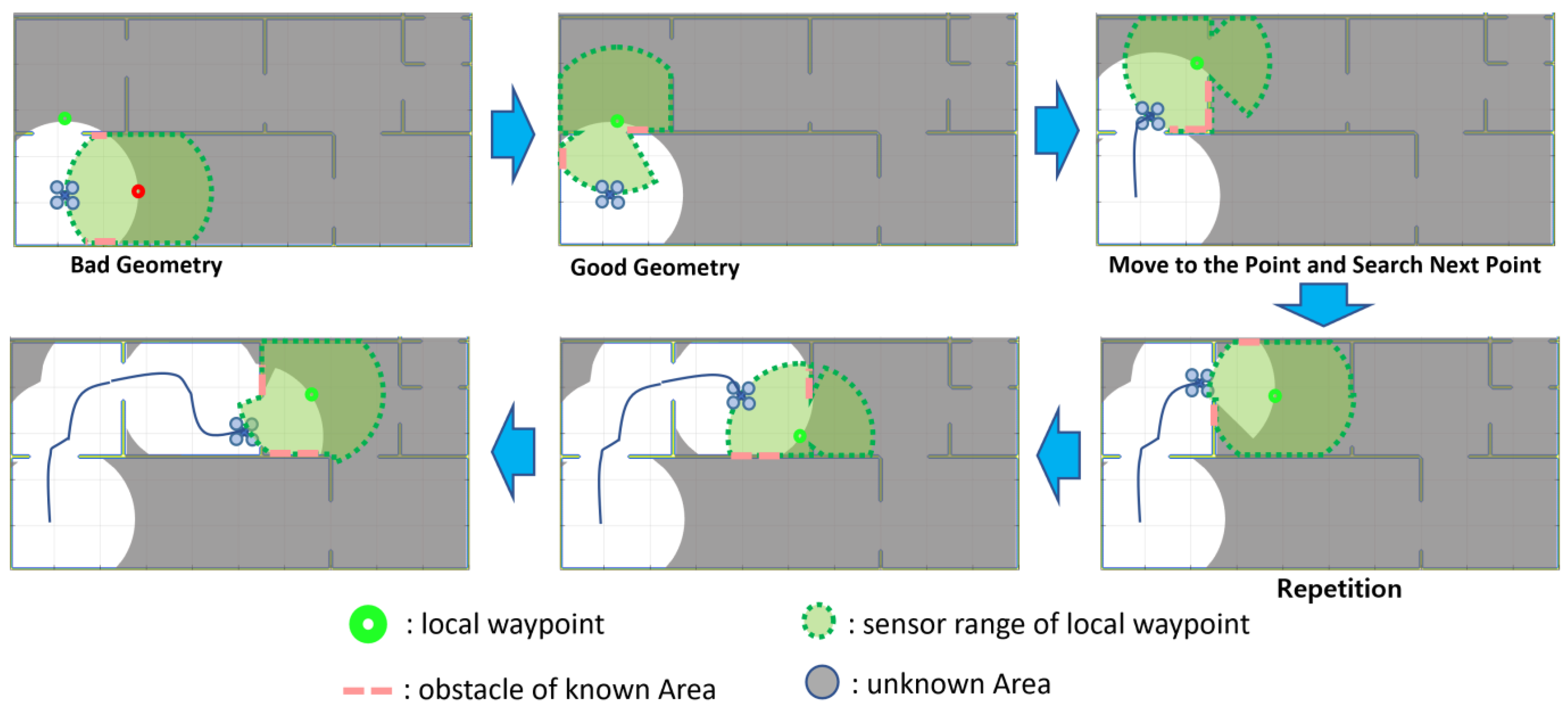
Figure 1 is a conceptual illustration of the exploration algorithm we propose, which involves selecting local arrival points in an unknown area. As SLAM explores unknown territory, it maps known territory. Using this map, it finds a location on the border of the unknown region where SLAM can perform well, and travels to that location. While traveling, SLAM continues to expand the known area, find another exploration point at the boundary of the unknown area, move to it, and so on. The exploration method presented in this paper applies the observability analysis technique to the exploration point and path generation process while securing the performance of SLAM. For path generation, the technique of [11] is used.

2.1. Three-Dimensional Point Cloud Map-Based Observability

Terrain features and obstacles play a very important role in SLAM’s position estimation. SLAM receives data from sensors about the surrounding terrain and extracts feature points to estimate position and attitude. If there are no features in the data, such as edges or lines, it will not be able to extract features. If there are no feature points, it will be impossible to match with the existing map and estimate the position. Therefore, the shape or geometry of the surrounding terrain has an important impact on SLAM. In this paper, we analyze the pseudo-observability of the surrounding terrain of a specific location to determine whether or not there is a problem in performing SLAM. For analysis, we calculate the rank and condition number of the proposed observability model.

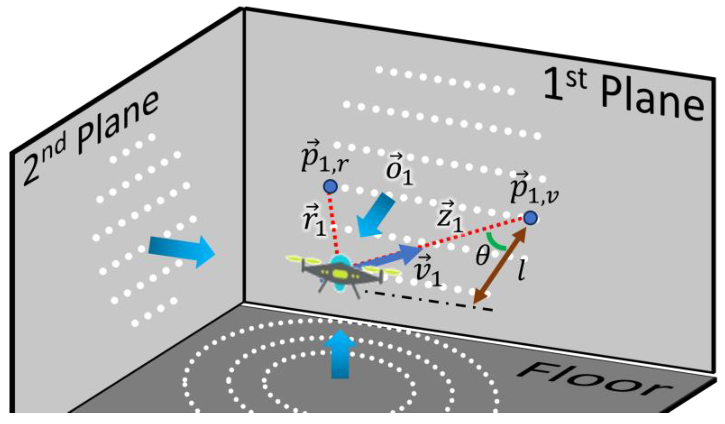
Figure 2 illustrates the measurement geometry when two walls are measured at a specific location, $\overrightarrow{P}$. In the figure, the blue area is the sensor measurement range, the black line is the wall, and the red dashed line is the detected wall surface. Here, the measurement Z is obtained based on the geometric relationship between a particular position, $\overrightarrow{P}$, and the wall. At the i-th wall measured at a specific location, $\overrightarrow{P}$, the measurement $z_i$ is obtained through two points, ${\overrightarrow{p}}_{i,r}$, and ${\overrightarrow{p}}_{i,v}$, and the observability is analyzed along with the perpendicular vector, ${\overrightarrow{o}}_i$, of the wall surface. Note that ${\overrightarrow{p}}_{i,r}$, and ${\overrightarrow{p}}_{i,v}$ are typically chosen to be the two endpoints of the wall, as this can lead to a singularity problem whenever the direction of the two points is parallel to the perpendicular vector, ${\overrightarrow{o}}_i$.

SLAM’s sensor data are highly dependent on the vehicle’s position and attitude. This is because the sensor data cannot observe walls, ceilings, etc., depending on the vehicle’s pose. To check the observability in the three-dimensional navigation area, the Lie derivative technique is employed for analysis. Here, the observability analysis takes position, $\overrightarrow{P}$, velocity, $\overrightarrow{V}$, and attitude, Φ, as state variables. Equation (1) shows the observability matrix for a single wall:

$${\mathcal{O}}_i=\left[\begin{array}{c}\nabla {\mathfrak{L}}^0{h}_i\\ \nabla {\mathfrak{L}}_{f_0}^1{h}_i\\ \nabla {\mathfrak{L}}_{f_2}^1{h}_i\end{array}\right]=\left[\begin{array}{ccc}\frac{{\partial \mathfrak{L}}^0{h}_i}{\partial \overrightarrow{P}}& 0_{1\times 3}& \frac{\partial {\mathfrak{L}}^0{h}_i}{\partial {\mathsf{\Phi }}_{\mathrm{b}}}\\ 0_{1\times 3}& \frac{\partial {\mathfrak{L}}_{f_0}^1{h}_i}{\partial \overrightarrow{V}}& \frac{\partial {\mathfrak{L}}_{f_0}^1{h}_i}{\partial {\mathsf{\Phi }}_{\mathrm{b}}}\\ \frac{\partial {\mathfrak{L}}_{f_2}^1{h}_i}{\partial \overrightarrow{P}}& 0_{3\times 3}& \frac{\partial {\mathfrak{L}}_{f_2}^1{h}_i}{\partial {\mathsf{\Phi }}_{\mathrm{b}}}\end{array}\right].$$

(1)

Here, $\nabla {\mathfrak{L}}^0{h}_i$ is the zero-order Lie derivative, which is the transfer function itself. Next, $\nabla {\mathfrak{L}}_{f_0}^1{h}_i$ is the first-order Lie derivative that takes into account position and velocity. Finally, $\nabla {\mathfrak{L}}_{f_2}^1{h}_i$ is another first-order Lie derivative expression that determines the effect of posture. For a system to be observable, a full-rank (Rank 9) condition is required. If one wall is observed, each element via position and velocity increases by 1 and attitude increases by 2 in rank. The rank increases as the vector ${\overrightarrow{o}}_i^T$ is newly defined along the X, Y, and Z axis directions. Now assuming i walls, the following observability matrix of a of size (5i) × 9 can be computed.

$$\mathcal{O}=\left[\begin{array}{c}{\mathcal{O}}_1\\ {\mathcal{O}}_2\\ ⋮\end{array}\right]=\left[\begin{array}{ccc}\frac{-{\overrightarrow{o}}_1^T}{{\overrightarrow{o}}_1^T·C_b^n{\overrightarrow{v}}_1}& 0_{1\times 3}& \frac{-{\overrightarrow{o}}_1^T·{\overrightarrow{r}}_1}{{\left({\overrightarrow{o}}_1^T·C_b^n{\overrightarrow{v}}_1\right)}^2}·{\chi }_1\\ 0_{1\times 3}& \frac{-{\overrightarrow{o}}_1^T}{{\overrightarrow{o}}_1^T·C_b^n{\overrightarrow{v}}_1}& \frac{-{\overrightarrow{o}}_1^T·\overrightarrow{V}}{{\left({\overrightarrow{o}}_1^T·C_b^n{\overrightarrow{v}}_1\right)}^2}·{\chi }_1\\ 0_{3\times 3}& 0_{3\times 3}& \frac{-{\overrightarrow{o}}_1^T·{\overrightarrow{r}}_1}{{\left({\overrightarrow{o}}_1^T·C_b^n{\overrightarrow{v}}_1\right)}^2}·{\left[{\chi }_1\right]}_{\times }\\ \frac{-{\overrightarrow{o}}_2^T}{{\overrightarrow{o}}_2^T·C_b^n{\overrightarrow{v}}_2}& 0_{1\times 3}& \frac{-{\overrightarrow{o}}_2^T·{\overrightarrow{r}}_2}{{\left({\overrightarrow{o}}_2^T·C_b^n{\overrightarrow{v}}_2\right)}^2}·{\chi }_2\\ 0_{1\times 3}& \frac{-{\overrightarrow{o}}_2^T}{{\overrightarrow{o}}_2^T·C_b^n{\overrightarrow{v}}_2}& \frac{-{\overrightarrow{o}}_2^T·\overrightarrow{V}}{{\left({\overrightarrow{o}}_2^T·C_b^n{\overrightarrow{v}}_2\right)}^2}·{\chi }_2\\ 0_{3\times 3}& 0_{3\times 3}& \frac{-{\overrightarrow{o}}_2^T·{\overrightarrow{r}}_2}{{\left({\overrightarrow{o}}_2^T·C_b^n{\overrightarrow{v}}_2\right)}^2}·{\left[{\chi }_2\right]}_{\times }\\ ⋮& ⋮& ⋮\end{array}\right].$$

(2)

However, in some cases, only one wall and floor on the horizontal axis can satisfy a full rank [12]. Therefore, we introduced the conditional number to determine the sensitivity of the matrix. Observability and conditionality are useful concepts for designing measurement strategies. Observability helps determine the minimum number and location of measurements for estimation, while conditional numbers help evaluate the accuracy and sensitivity of measurements. Typically, the conditional number in the observability matrix can be used as an indicator of the degree of observability [13].

Now, let ${\delta }_{max}\left(\mathcal{O}\right)$ and ${\delta }_{min}\left(\mathcal{O}\right)$ be the maximum and minimum singular values of the observability matrix. Dividing these two singular values gives the conditional number, $\kappa \left(\mathcal{O}\right)$, of the observability matrix, as shown below:

$$\kappa \left(\mathcal{O}\right)={\delta }_{max}\left(\mathcal{O}\right)/{\delta }_{min}\left(\mathcal{O}\right).$$

(3)

As the condition number becomes smaller, each row and column of the observability matrix becomes more independent, and thus more robust in estimation. Based on this principle, we can measure the degree of local observability via the conditional number of the observability matrix.

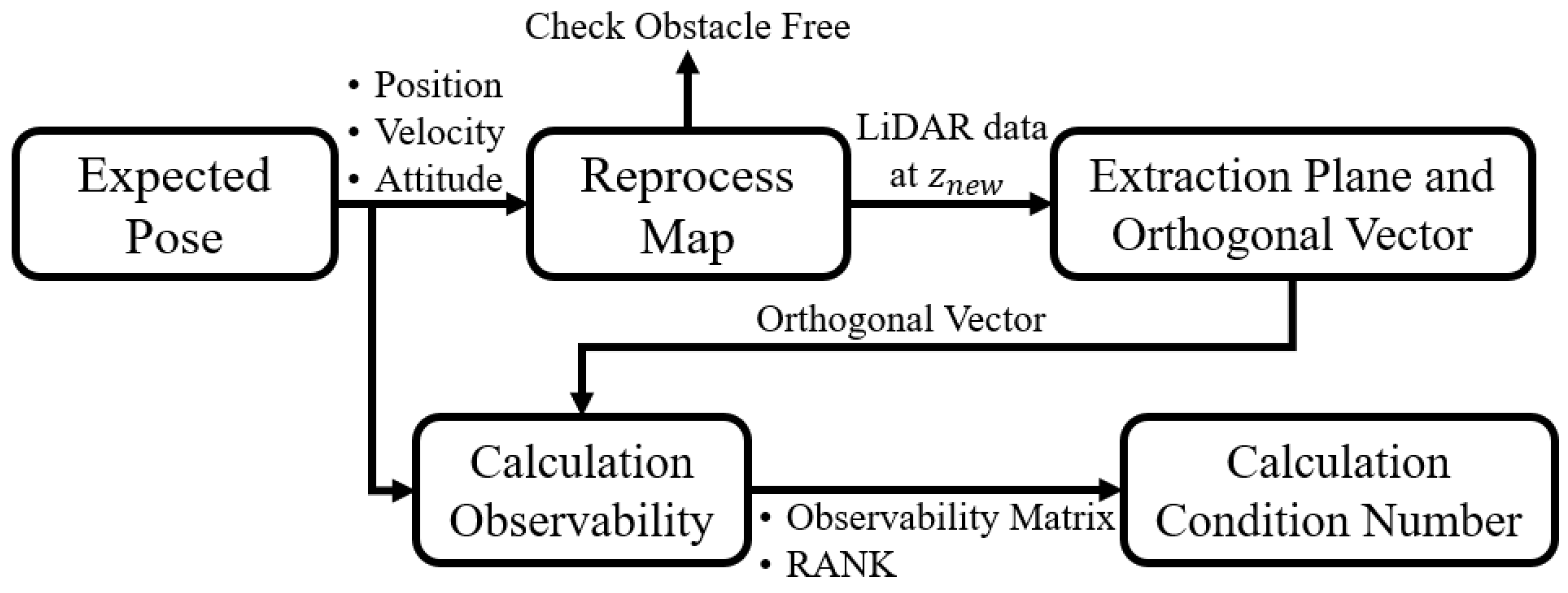
In this study, we propose a method to analyze the observability of a specific location. Observability is an important factor to ensure the performance of SLAM. The overall block diagram of the proposed algorithm is shown in Figure 3.

The procedure is as follows. First, take the specific location and map information as input to estimate the predicted velocity and attitude. Second, using the specific location on the map and the predicted attitude, generate the expected sensor data when the aircraft is at the specific location. Third, detect walls using LiDAR from the generated sensor data and obtain the normal vector of the walls. Fourth, construct an observability matrix using the normal vector of the wall as an input, and calculate the rank and condition number of this matrix to quantify observability. These quantified values can be used as indicators to evaluate the performance of SLAM at a specific location.

2.2. Boundary Extraction Techniques with Unknown Areas

For exploration, it is important to first find the boundary between known and unknown areas. This is because the boundary allows us to calculate the next exploration location. The algorithm for finding the boundary is partially based on the method in [6]. The method for finding the boundary between the known and unknown regions works in two ways.

The first is the global RRT, which creates a tree from the initial position of the vehicle and continues to create branches within the known area until the end of the exploration. If it detects an unknown region at the end of the branch, it stores the location in E(n) and continues to perform unknown region detection. The second is the local RRT, which starts at the vehicle’s current location and continues to create branches within the known area. When it detects an unknown region, it stores its location in E(n) and restarts the local RRT, i.e., when it detects an unknown region, it clears the branches and rebuilds them from the vehicle’s current location.

Global RRT detection creates branches throughout the known region, so that every region recognizes the boundary with the unknown region. Local RRT detection allows us to know the location of the boundary with the unknown region in the area close to the vehicle.

The boundary points between the known and unknown regions obtained by the unknown region detection algorithm are plotted as candidate exploration points. In Figure 4, the white dots represent candidate exploration points. Then, the procedure is established as follows: first, place the candidate group at a specific location, $\overrightarrow{\mathrm{P}}$; then, calculate the condition number of observability; finally, proceed to a nearby location with a low condition number as a waypoint for exploration.

3. Exploration Point Creation Techniques

The exploration algorithm figures out where the unknowns are and approaches them to make them known. If there are multiple unknowns, there is a need to prioritize which ones to approach. Therefore, the race between the unknown and known areas is a candidate for exploration points, and the exploration points are selected through analysis. Algorithm 1 below illustrates the proposed exploration algorithm that partially incorporates the Frontier-based exploration concept [5,7].

Algorithm 1. Select Exploration Point.

1: $\left(M_{octo},S\right)\leftarrow MapConv$ 2: $\mathit{f}\mathit{o}\mathit{r}i=1toi=Ndo$ 3:     $N_{cond}\leftarrow Observability\left(M_{octo},E\left(i\right)\right)$ 4:     $\mathit{i}\mathit{f}1\le N_{cond}\le N_{max}Then$ 5:         $\mathcal{I}\leftarrow Near\left(E\left(n\right),E\left(i\right),r\right)$ 6:         $d\leftarrow dist\left(P_v,E\left(i\right)\right)$ 7: $P_{min}\leftarrow MinCost\left(\mathrm{K},\mathcal{I},d,E\left(i\right),P_{min}\right)$ 8: $\mathit{e}\mathit{n}\mathit{d}\mathit{i}\mathit{f}$ 9: $\mathit{e}\mathit{n}\mathit{d}\mathit{f}\mathit{o}\mathit{r}$ 10: $\mathit{r}\mathit{e}\mathit{t}\mathit{u}\mathit{r}\mathit{n}{P}_{min}$

MapConv$\left(\right)$: A function that takes a point cloud map from SLAM and returns an octomap, $M_{octo}$, and map size, S. octomap is an octree-based map that has the strong advantages of fast searching and efficient memory management. The reason for converting to Octomap is to detect walls before computing observability.

Observability$\left(\right)$: A function that calculates the observability and condition number, $N_{cond}$. By centering on the node position, $z_{new}$, it uses the raycasting technique to find nearby walls. It also serves as an obstacle avoidance function by returning 0 if a wall or obstacle is too close. For this, it requires the extraction of orthogonal vectors from the detected walls and the use of the extracted orthogonal vector and the position of the vector to make observations and calculate the condition number, $N_{cond}$.

Near$\left(\right)$: A function that determines the number of prospect candidates, $E\left(n\right)$, in the neighborhood of prospect candidate $E\left(i\right)$. A large number of candidates in the neighborhood means that when the drone goes to this point, it can cover a larger area, extending into a known area.

$\mathit{d}\mathit{i}\mathit{s}\mathit{t}\left(\right)$: A function to find the Euclidean distance between a candidate exploration point E(i) and the vehicle’s position, $P_v$. The following formula is $=\sqrt{{\left(x-x_v\right)}^2+{\left(y-y_v\right)}^2+{\left(z-z_v\right)}^2}$, where x, y, and z are the position values of $E\left(i\right)$ and $x_v,y_v,z_v$ are the position values of $P_v$.

$\mathit{M}\mathit{i}\mathit{n}\mathit{C}\mathit{o}\mathit{s}\mathit{t}\left(\right)$: A function that calculates the cost of a prospect and returns the location of the smallest prospect. This calculates the cost and returns the location value of $E\left(i\right)$ if it is less than the cost of the existing $P_{min}$. The cost calculation formula is $\mathrm{G}\left(\mathrm{d},\mathcal{I}\right)=K_{d}d+K_{\mathcal{I}}\mathrm{s}\mathrm{i}\mathrm{z}\mathrm{e}\left(\mathcal{I}\right)$, where K is the gain.

Algorithm 1 is the methodology for determining the next exploration point. Among N candidate exploration points, we find the one with the lowest cost and move it. First, the number of geometric observability conditions of the candidate exploration points is calculated. If the number of conditions is greater than or equal to N_max, the navigation performance of the location cannot be guaranteed. Therefore, only candidate exploration points with N_max or less are used. Among these candidates, the robot selects the best candidate using the Near, dist, and Mincost functions. Algorithm 1 starts computing when the robot arrives at the previous exploration point.

When creating exploration points, it is problematic if the exploration points are in areas where navigation performance is not guaranteed. Therefore, we perform an observability analysis on the candidate exploration points and exclude the candidates with poor conditions from the exploration points. When the vehicle arrives at a probe point, it pauses and looks for the next probe point. Since the vehicle is paused, its velocity is 0 and its attitude is roll 0° and pitch 0°. Therefore, no attitude and velocity estimates are used in the observability analysis of candidate exploration points.

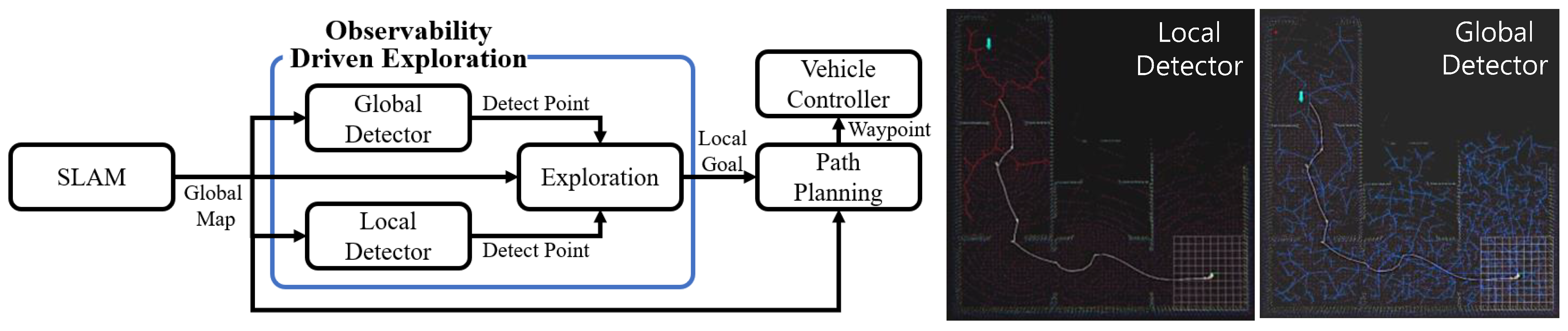
In the known and unknown region boundary detection technique, global RRT and local RRT are performed exclusively, where the exploration region is separated. First, local RRT draws candidate exploration points from the boundaries of the unknown area that are located close to the vehicle, which are temporarily used in each iteration. Global RRT takes the role of finding candidate exploration points including both explored and unexplored regions beyond the local RRT region. In the case that exploration point candidates from the global RRT distribute evenly from the boundary of the unknown area, higher scores can be assigned during exploration for point candidates that are closer to the vehicle. The algorithm block diagram and paths are exemplified in Figure 5.

The exploration point generation algorithm is performed when the vehicle arrives at a previous exploration point. The exploration target locations generated by this algorithm are passed as arrival points to the path planning technique in [11] to drive the path while ensuring navigation performance. This operation is repeated to complete the exploration.

4. Simulation Study

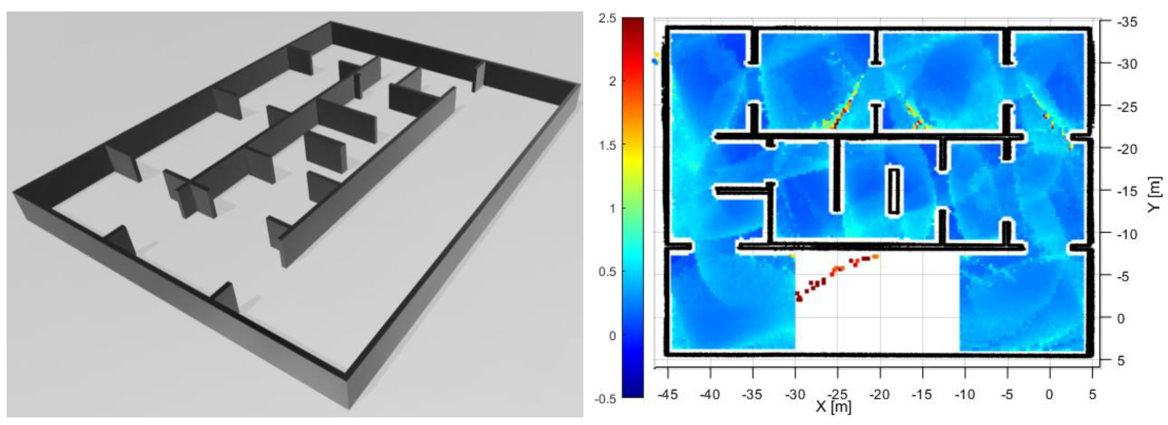
For validating the proposed observability-based exploration method, we first performed simulation works. Simulation allowed the vehicle to move autonomously and explore a virtual environment. Figure 6 shows a new environment created in the Gazebo simulator to determine observability. As shown in the figure, we prepared three types of corridor: a corridor with no obstacles from the bottom, a corridor with complex obstacles, and a corridor with simple obstacle gates.

It has been shown in [9] that LiDAR SLAM does not estimate its position and diverges when the robot is between (−30, −7.5) and (−10, 5), as shown in the bottom region of Figure 6. Therefore, we tested the proposed algorithm in the same map environment to verify whether or not the exploration can be successfully completed without navigation divergence. We also set the sensor range to 15 m and calculated the number of conditions in regular intervals. As shown in the previous figure, the lower the number of conditions, the more intense the blue color, and the more intense the red color, the better the number of conditions for navigation. In the figure, we can see that in the area with obstacles, the number of conditions is calculated as the full rank is reached and the number is low. However, in the area without obstacles, the number is high even if it is not a full rank in the middle.

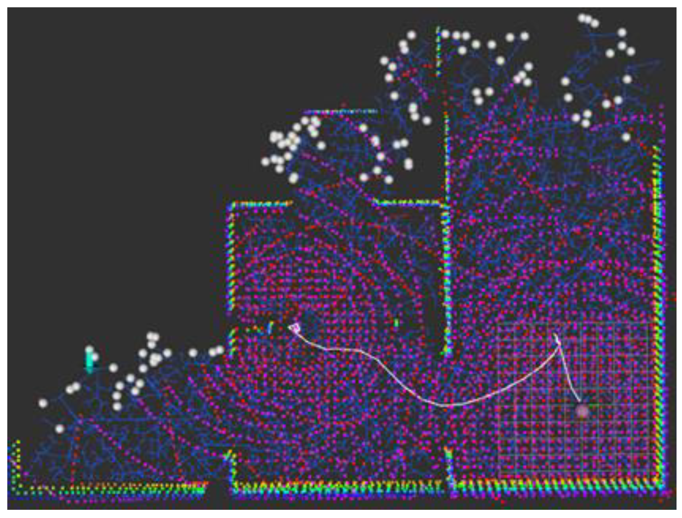
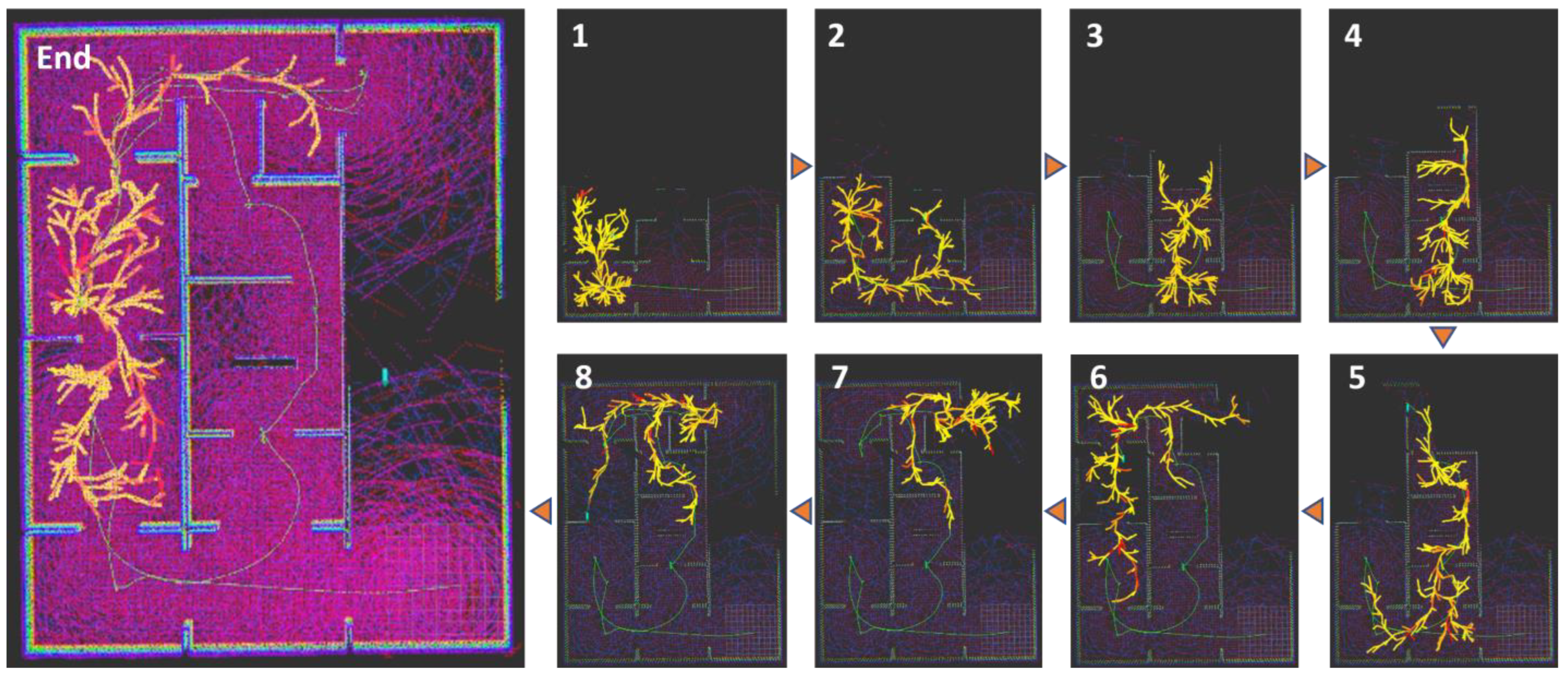
In Figure 7, the black color is the unknown area and the purple color is the known area. The green color is the wall and the light-green line is the path the vehicle traveled. The yellow and red lines are the RRT* branches generated by the path planning algorithm. They are colored differently based on the condition number. The higher the condition number, the more the color changes from yellow to red.

In this simulation, we can see that the unobstructed path on the left was explored. The reason why the unobstructed path was not explored can be found in the condition map in Figure 6. In Figure 6, you can see that the conditionals are not computed in the lower part of the unobstructed path. This is because the observability matrix is not full-rank in that region. For the same reason, the path on the left in Figure 7 is not guaranteed to be observable, so the condition number cannot be computed and it is not approached. This is a double-check of the exploration points as it is applied in both the exploration point generation and path planning algorithms. Simulations were performed to see how exploration is performed by the exploration algorithm and to check the error performance of the navigation. We analyzed the impact of the maximum distance of LiDAR on the navigation and exploration algorithms. The maximum distance of LiDAR was set to 50 m, 20 m, and 10 m, and exploration was performed in a simulation environment. The exploration algorithm used LIO-SAM [14] to generate a map and plan a path. The condition number of waypoints generated along the path was color-coded to compare the coverage and observability. The performance of the vehicle driving the path was also evaluated.

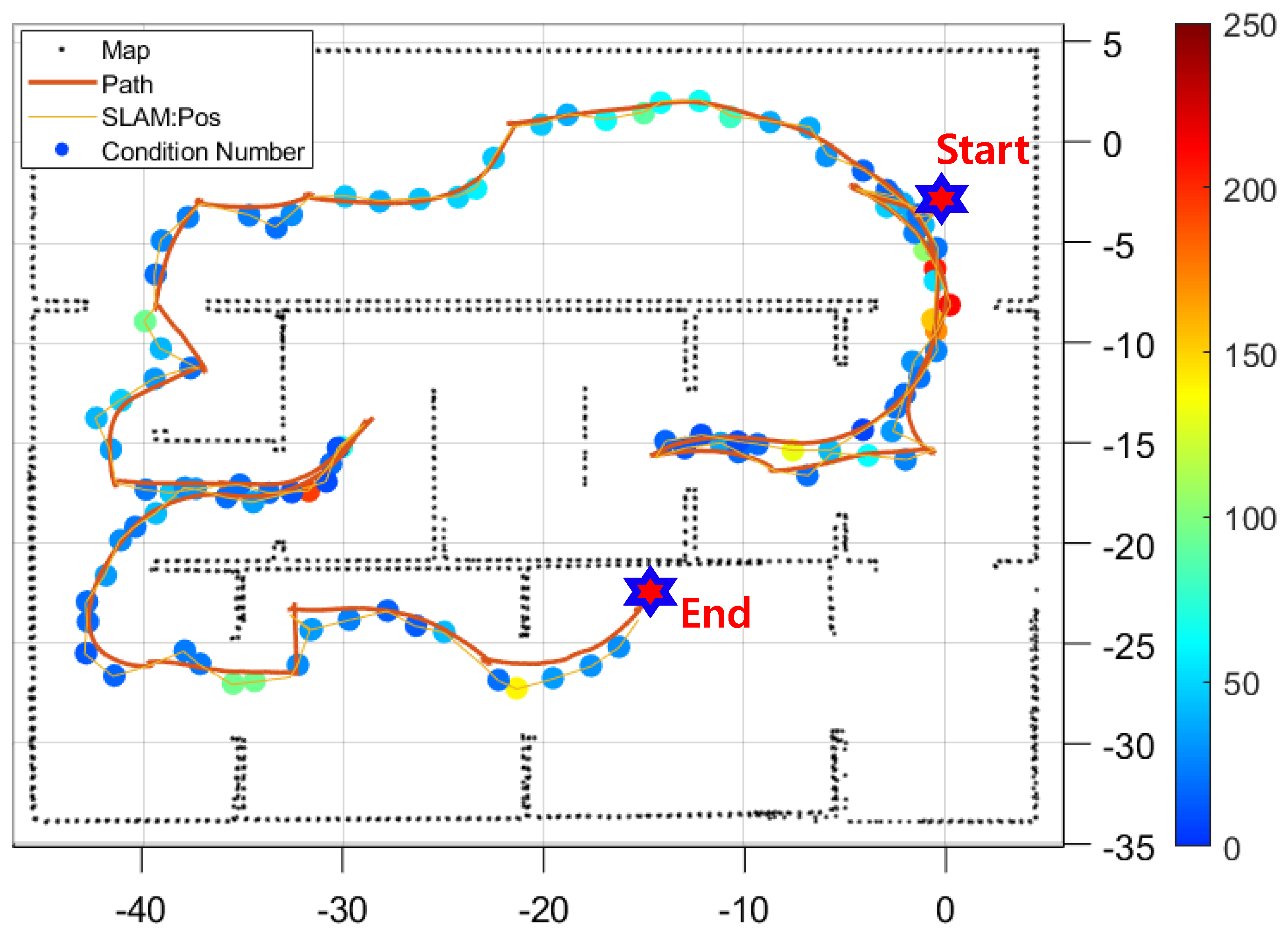
4.1. LiDAR Max Range: 50 m

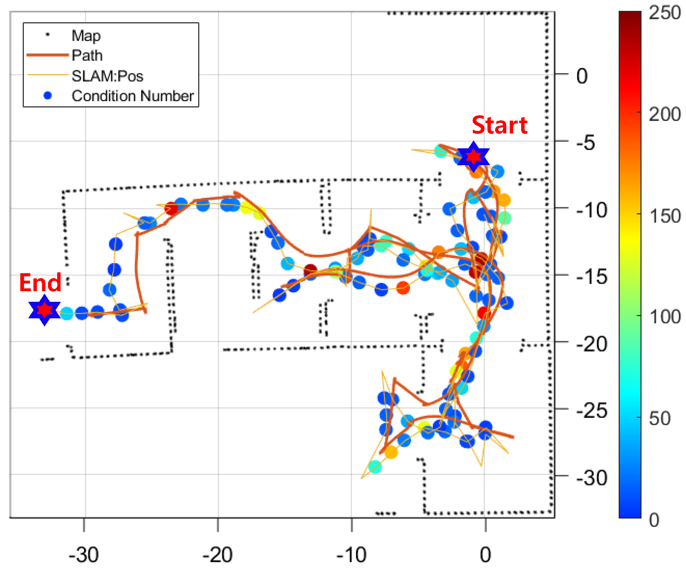
Figure 8 shows the exploration results as a function of LiDAR’s maximum distance. The black dots represent the map and the orange line represents the vehicle’s position estimate. The yellow line represents the path generated by the exploration algorithm, and the colored dots represent the condition numbers of the waypoints. Higher condition numbers are colored red and lower condition numbers are colored blue. In the figure, we can see that inside the rooms, the condition numbers are low and colored blue, while the condition numbers increase at the boundaries between rooms. This is due to the terrain at the boundary, which prevents LiDAR from covering a large area, resulting in a higher condition number.

Looking at the graph of the calculated condition number at each waypoint, we can see that the condition number is below 100 throughout, indicating good observability. This is because the simulation environment is 50 m by 40 m, so if LiDAR has a maximum range of 50 m, even if the vehicle is at the end of the room, it can measure to the opposite wall. Therefore, no matter where the vehicle is located, all four sides of the horizontal plane are measured, so observations are possible and the condition number is low.

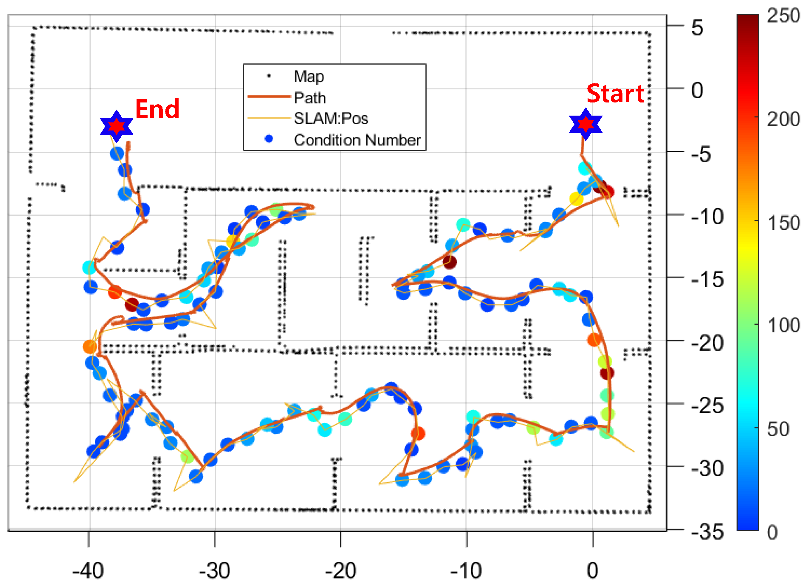
4.2. LiDAR Max Range: 20 m

Assuming varied range performances among LiDAR sensors, we first considered a measuring range of 20 m. In a typical LiDAR, it is the distance at which an object with 10% reflectivity can be measured.

The representation for the graph in Figure 9 is the same as that in Figure 8. If you look at the paths generated in the above figure, you can see that the exploration algorithm does not enter the center of the upper pathway, but turns around and approaches it. This is because LiDAR has a maximum range of 20 m, so for the upper path, any location more than 20 m away from the walls on either side is at risk of diverging navigation. Hence, you can see a path that avoids that area. Most waypoints have low condition numbers, but some locations have high values. These locations correspond to the boundaries between rooms and are analyzed as shaded areas due to obstacles, which increase the condition number. It can be seen that as the maximum distance of LiDAR decreases, the number of walls that can be measured decreases and the maximum value of the condition number becomes relatively large.

4.3. LiDAR Max Range: 10 m

We evaluate the performance of our exploration algorithm by limiting the maximum measurement range of the LiDAR to 10 m. We carry this out because limiting LiDAR’s measurement range reduces observability and reduces exploration efficiency.

In this simulation, we can see that the LiDAR maximum range is short, so there are fewer obstacles that can be measured at once, resulting in a lot of empty space during the map generation process, which causes problems in generating exploration points and paths. This can be seen in Figure 10, where the map is not fully formed compared to the previous results. The condition number is an indicator of SLAM’s navigational estimation potential based on the geometry at the waypoint, with smaller values being better. As can be seen in the graph, most of the waypoints have small condition numbers. This means that the algorithm is designed to explore places with low conditionals, despite the limited maximum measurement range of LiDAR.

5. Experimental Result in Real Field

To further validate the performance of the proposed exploration algorithm, we conducted experiments in a real-world environment. In this way, we could check the exploration efficiency, stability, etc., of the exploration algorithm in a real environment. The exploration area was set to 20 m wide and 20 m long to perform the exploration algorithm. The sensors used in the experiment are OS0-32 LiDAR from Ouster and VN-100 IMU from Vectornav. The computing device was a NUC11PAHi7 from Intel, and the environment was set to ubuntu 18.04.

5.1. LiDAR Max Range: 50 m

In the experiment, we set the maximum LiDAR range to 50 m, which is the maximum distance of OS0-32, and SLAM used the Lio-SAM algorithm to explore. We then checked the results of driving along this exploration path with the maximum LiDAR distance set to 10 m.

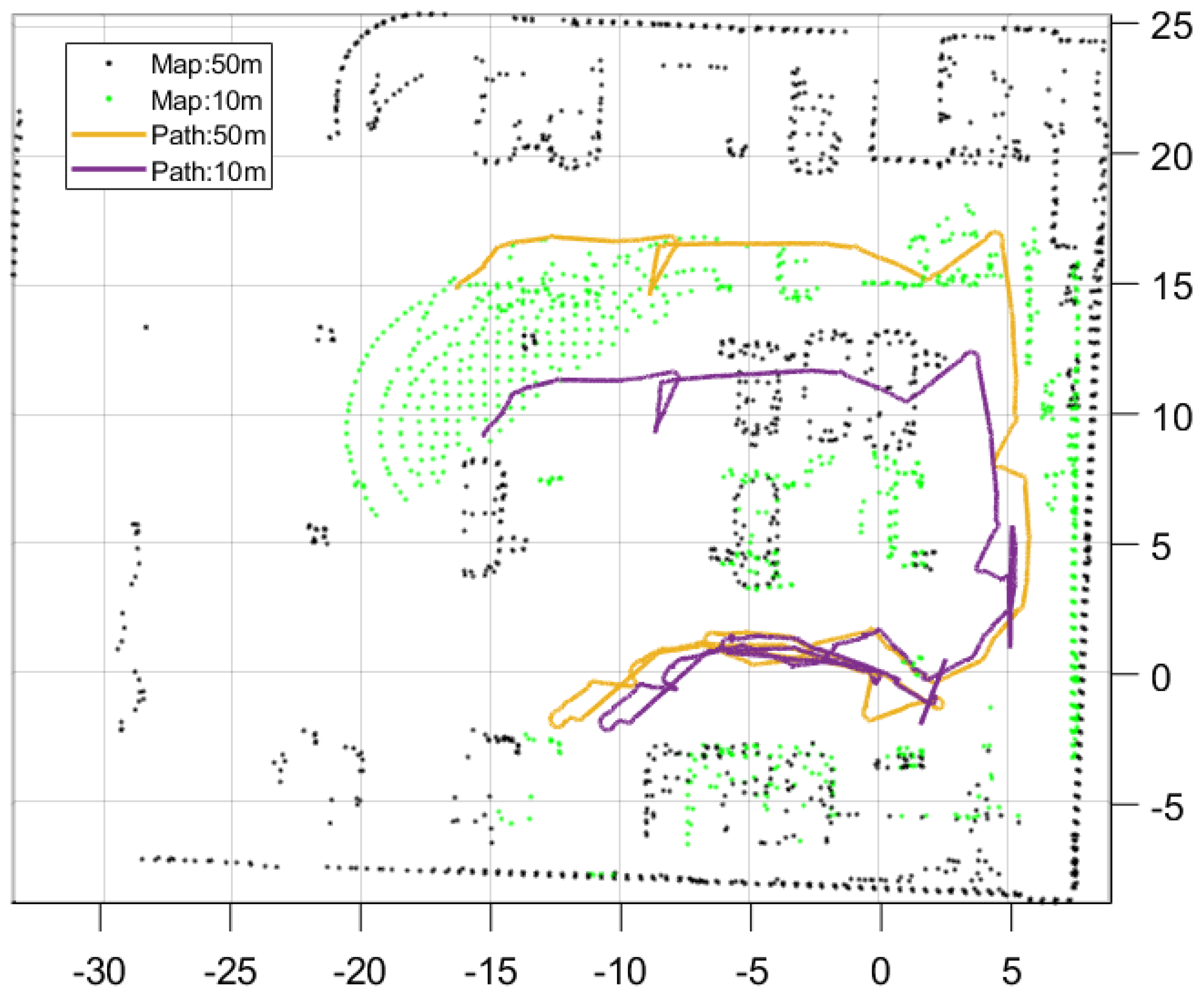
Figure 11 shows the path generated by the exploration algorithm and the map generated by driving the path. The black dots and orange lines show the map generated by SLAM [12] and SLAM’s position estimate when the LiDAR maximum distance is 50 m. The green dots and purple line show the map generated by SLAM and the SLAM’s position estimate when the LiDAR maximum distance is 10 m. Both conditions are the result of adjusting only the maximum LiDAR range on the same dataset. We can see that the error is significant in situations where the sensor’s performance is limited.

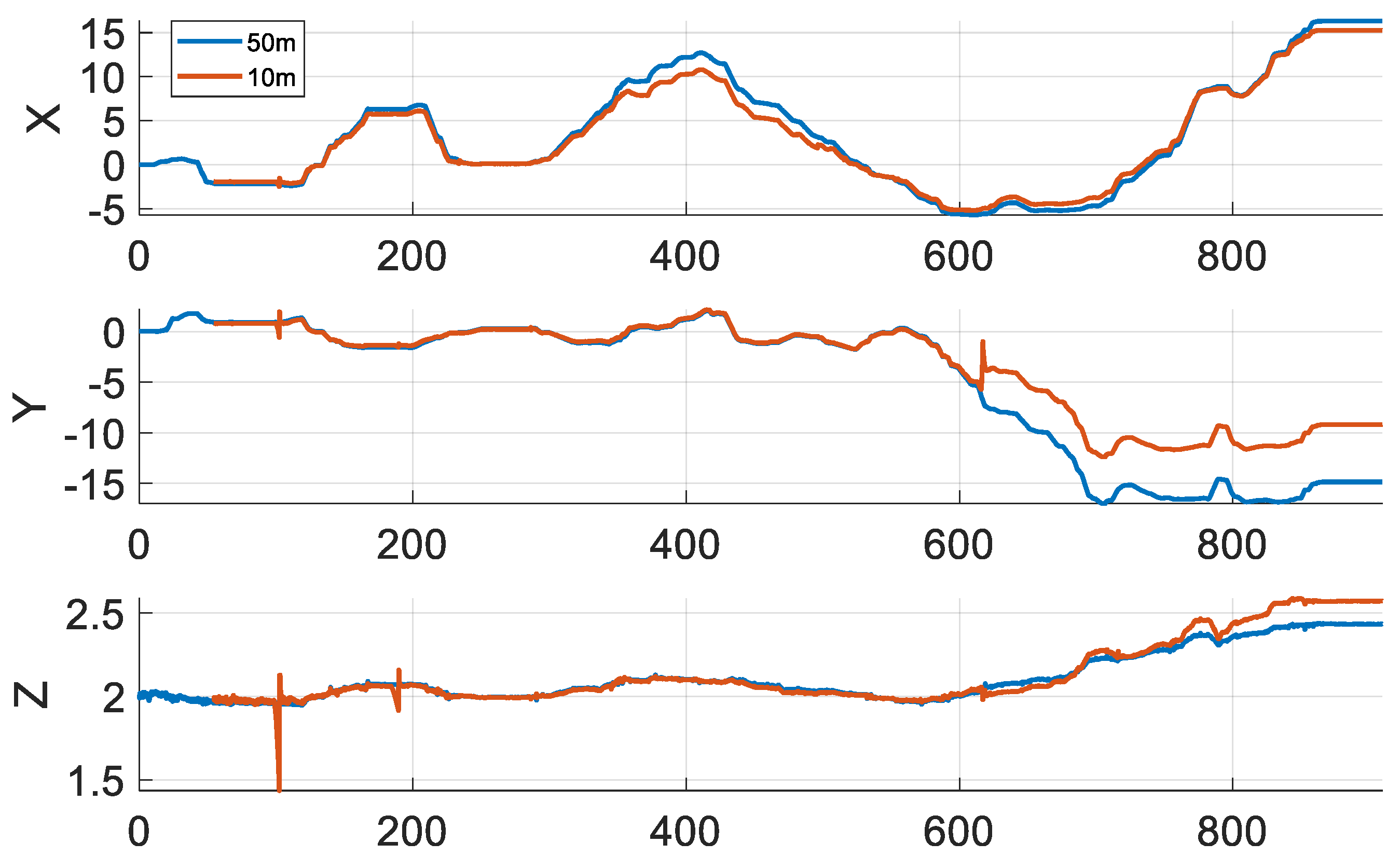
Figure 12 shows the position results from Figure 11 graphed over time. In this graph, we can see that errors occur and accumulate around 100 s, 350 s, and 610 s. This suggests that the lack of sensors in certain areas causes a large error in navigation. Therefore, there are areas where navigation does not perform well, and the error is large.

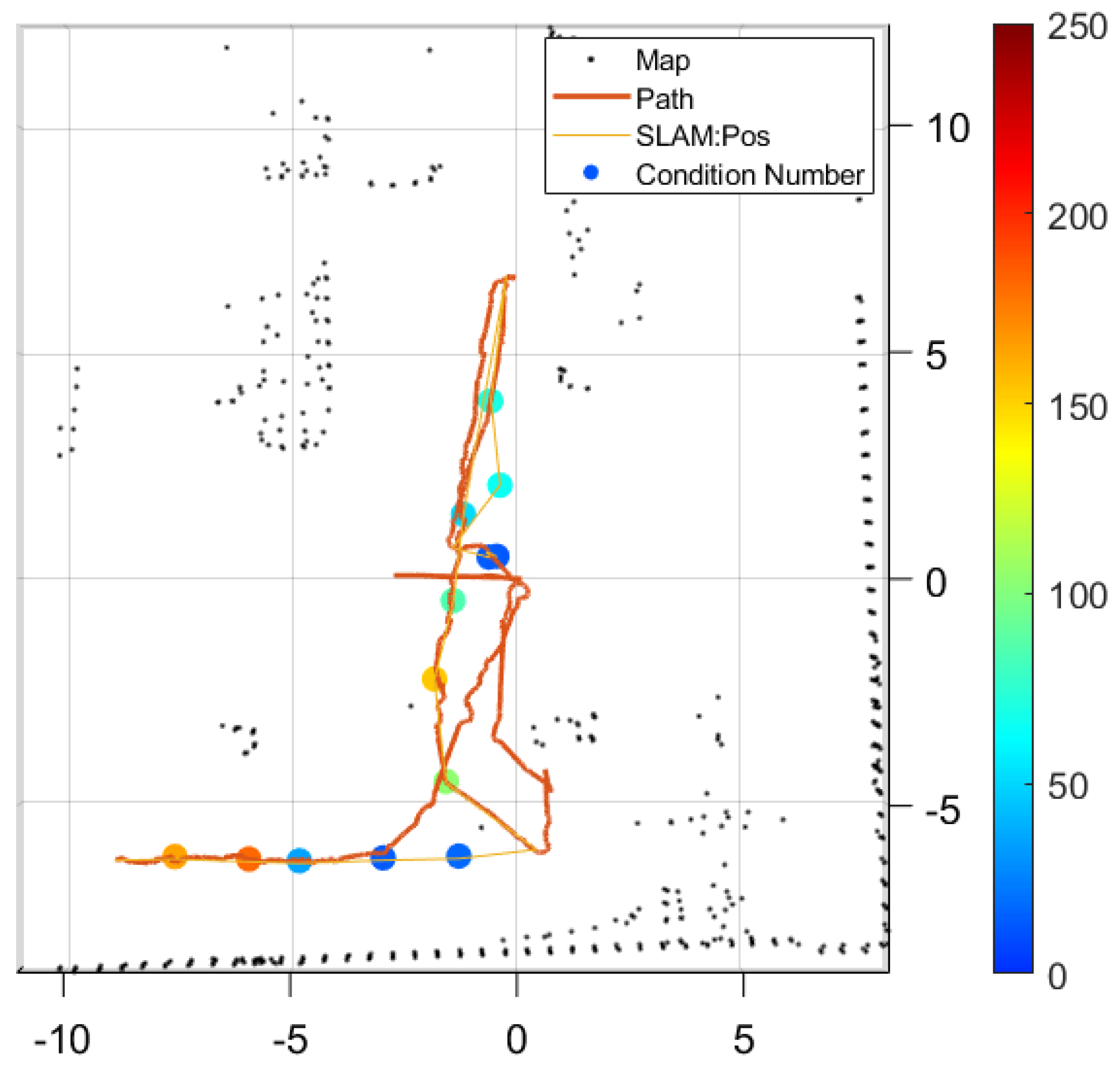
5.2. LiDAR Max Range: 10 m

In the second experiment, we set the maximum range of the LiDAR to 10 m, where the accuracy of OS0-32 was measured with a performance of ±1 cm. SLAM was explored using the same Lio-SAM algorithm as that in the previous experiment. For this experiment, we analyzed how the smaller sensor range affects map generation and exploration planning. The initial starting position, attitude, and exploration conditions are the same as those in the previous experiment.

Compared to those in the previous experiments, we can see that the maps generated are smaller and the areas explored are smaller. This means that as the sensor measurement range decreases, the size of the generated map decreases, and the area determined to be explorable decreases. You can also see that the number of conditions that were previously increased (Figure 13).

6. Conclusions

In this study, we proposed a new method that introduces observability characteristics to ensure the performance of LiDAR SLAM. The observability characteristics are defined as a matrix that reflects the features of the environment that can be observed by the LiDAR sensor, and we used it to determine the suitable location for LiDAR SLAM; we evaluated the stability of LiDAR SLAM using the condition number of the observability matrix. We also proposed a path planning and exploration algorithm for LiDAR SLAM using observability characteristics. We experimentally verified that the algorithm can respond to various environments and obstacles using a simulator and a UGV.

This study applied observability characteristics to a three-dimensional point cloud map, but it was not applied to dynamic environments or multiple LiDAR sensors. Further research is needed to overcome these limitations. In the future, we plan to study how to apply observability features to other types of maps, study how to update or calibrate observability features in dynamic environments, and study how to calculate or distribute observability features across multiple LiDAR sensors. This is expected to further improve the performance and versatility of LiDAR SLAM.